
Submitted:
07 January 2026
Posted:
08 January 2026
You are already at the latest version
Abstract
People in mid-life interact with several different environments during their daily life in-cluding employment, leisure, commuting, and various family responsibilities, a concept defined as activity space. However, little is known about how these activity spaces contrib-ute to individuals’ daily health behavior choices. The Everyday Environments and Expe-riences (E3) study was conducted to explore these relationships. In this paper, we provide a reproducible GPS processing workflow to generate time-weighted exposure measures (activity spaces) inferred from 21 days of continuous GPS monitoring among 340 mid-life adults in Cook County, Illinois (N=340) from the E3 study. Data from waist-mounted GPS devices that recorded one-minute location epochs were aggregated after excluding time spent within an 800-meter buffer around the home. For each epoch, we derived proximity and kernel density measures for eleven food and physical-activity-related location types (e.g., supermarkets, fitness facilities), along with twenty-six environmental context varia-bles (e.g., land use, crime, population density). Time-weighted averages characterized each participant’s typical non-home environmental exposure. After adjustment for envi-ronmental context, age and gender were generally unrelated to activity-space measures. However, Black and Hispanic participants (as compared to White participants) spent less time near both food and physical-activity resources, suggesting systemic inequities in ac-cess beyond neighborhood composition.
Keywords:
exercise
; physical activity
; urban
; systemic inequity
1. Introduction
Unhealthy dietary and physical activity (PA) behaviors contribute to an increased risk for obesity, cancer, and other aging related chronic diseases [1,2,3]. These behaviors further accentuate health disparities [4], especially during the transitional period of mid-life. Mid-life is a known vulnerable life stage when obesity rates peak and chronic diseases emerge, often related to modifiable lifestyle risk factors [5,6]. Residential neighborhood environments provide opportunities, barriers, and cues/triggers to engage in healthy or unhealthy behaviors, making them a focus of built environment public health research. Interventions and policies that impact neighborhood-built environment on public health are a major focus Healthy People 2030 [7]. However, research findings on residential neighborhood environment-behavior associations are inconsistent and effect sizes are small [8]. One potential explanation is that additional environmental exposures during daily living contribute to levels of healthy behaviors. Much of the current research on residential neighborhoods does not consider the activities of daily living in mid-life.
People in mid-life interact with several different environments during their daily life including employment, leisure, commuting, and various family responsibilities, a concept defined as activity space [9]. Failure to consider these activity spaces – the full daily exposure to various environments – may cause research to date to miss the full impact of environmental differences on health behaviors. Quantifying aspects of an individual’s activity space is necessary to understand whether activity spaces do in fact impact health behavior, and how these explanations may vary based on other individual and environmental factors. To date, little is known about the putative impact of activity space on health behavior, and how best to measure and quantify activity spaces.
The purpose of the Everyday Environment and Experiences (E3) study is to provide methodological innovation on how to measure and quantify activity spaces, while investigating how activity-space may explain participant variations in diet and PA during mid-life [8]. To do this, enrolled E3 participants wore global positioning system (GPS) tracking devices for 21 continuous days. In this manuscript, we detail a novel, reproducible, and robust method of how GPS inferred position information on participants was extracted and summarized into summaries of activity-space. Activity-space-inferred data includes availability of healthy and unhealthy foods, walkability and recreational resource availability (e.g., parks, fitness facilities, greenness). We illustrate how these activity space measures differ across participant characteristics, suggesting potentially generalizable conclusions about gender, age and race/ethnicity differences associate with different lived experiences as quantified by activity space data. We also show how these relationships may be explained by other characteristics of the activity space (e.g., crime, poverty, population density).
2. Materials and Methods
2.1. Study
The full details of participant recruiting and participation in E3 are described elsewhere [10], but we summarize them briefly here. Individuals eligible for this study met the following criteria: (1) self-reported as non-Hispanic (NH) White, NH Black or Hispanic/Latino; (2) aged 40 to 64 years; (3) resided in Cook County, Illinois; (4) had access to a smartphone; (5) provided informed consent. Participants were recruited using a variety of community focused recruiting methods and ultimately resulted in an enrolled sample of 400 participants. Interested participants first underwent a recruitment call with a staff member to learn about what the study entails and ensure eligibility. The study was approved by the University of Illinois Chicago Institutional Review Board (IRB 2019-0630) and informed consent (e-consent) was obtained prior to study procedures.
2.2. GPS Protocol and Data Collection
As discussed in Bronas et al. 2025 [10], after enrollment, data collection for the E3 study occurred in three stages: a baseline visit, the three-week (21 day) study period, and a follow up visit, all of which were performed remotely. Prior to the baseline visit, each enrolled participant received a Global Positioning System (GPS) device by mail. At the remote baseline visit participants completed short interviews and were trained/prepared for all components of data collection, including training on how to use and wear the GPS unit. After 21 days, participants ceased data collection and had a remote follow up visit. The GPS device was then shipped back to the main study location, where participant data was downloaded and catalogued.
The GPS units participants received were Qstarz BT-Q1000XT Bluetooth Data Logger Receivers (Qstarz, Taipei, Taiwan). Participants were instructed to wear the GPS unit around their waist via a hook and loop fastened waistband for the entire 21-day study period. Each GPS unit was set to measure participant position at 1-minute epochs. Participants were instructed to always wear the waistband except when swimming, bathing, or sleeping, and to charge the device with the provided charger when it was removed for sleeping. Some modest non-compliance to these instructions was noted over the course of the study, including failure to wear the device at home, when going out, or while working, and neglecting to charge the device overnight then charging during the day when the device should be worn (the typical battery life is 42 hours). In one case, a participant's GPS device was not functioning properly and needed to be replaced. In sum, of the 400 participants enrolled in the E3 study, 362 GPS records were retrieved from returned devices, 347 of which had measurable data during the 21-day study period.
Raw data from the 347 participants was stored in comma-separated value (csv) files, including latitude and longitude coordinates with date and time stamp for each minute (epoch) the device was monitoring. Using R (version 4.2.0; R Core Team 2022), we truncated the raw csv files to the study time frame (baseline visit date to 21 days) and used the AGPSR package [11] (Step 2) to clean and impute the coordinate data. Specifically, using AGPSR, we removed any location epoch that implied a speed of >130 km/h from the previous epoch. We also removed epochs outside of a pre-specified set of fourteen counties covering the Chicago metro area, (Illinois: Cook, Dekalb, Du Page, Grundy, Kane, Kendall, Lake, McHenry; Indiana: Will, Jasper, Lake, Newton, Porter; Wisconsin: Kenosha), allowing 7 minutes after a participant left the area before starting to drop data points. Accordingly, any epochs suggesting a position in Lake Michigan were removed 7 minutes after the last time the participant was positioned in an appropriate county. We then linearly interpolated any sequence of 5 or less missing points between two observed points. After applying the AGPSR function for data cleaning and imputation, we also removed data for 7 participants who had no record of their GPS device traveling farther than 800 meters from their home address by street network.
2.3. GPS Inferred Activity Space Measures
Using the remaining 340 GPS records (Figure 1), we provided geographical context to every epoch via the ESRI GIS processing tool and database ArcGIS (Pro version: 3.1.3). To prepare the GPS data and apply the ArcGIS tools, we implemented the ArcPy package in Python. We first geocoded the participants' home addresses to GPS coordinates, then defined an 800-meter buffer around each home location by street-network, meaning the resulting polygon had at most a distance of 800 meters via roadway from edge to the center location. For each remaining epoch, we computed the closest distances to eleven location types (public park, bike path segment, physical activity location, pedestrian segment, public transit, street intersection, convenience store, any fast food restaurant, fast food chain restaurant, supermarket and wholesale club store). We also computed kernel densities (per square mile) for each epoch for the same eleven location types [7]. Kernel density surfaces were fit for each location type across the Chicago metro area using the ESRI Spatial Analyst Toolbox, which implements a quartic kernel function [12]. Figure 2 illustrates the kernel density surface estimate for convenience stores for the fourteen counties included in this study. Casually, Figure 2 illustrates how dense convenience stores are at any given location across the fourteen-county area (darker red=more dense), allowing us to obtain a kernel density value for convenience stores for each epoch for each participant. The kernel density value of an epoch is calculated for a 100-meter raster cell from an overall grid. Thus, we created a total of 22 separate measures of activity space (11 distance measures; 11 kernel densities (per square mile)) for each epoch.
2.4. GPS Inferred Environmental Context Measures
We also obtained twenty-six additional environmental context measures for each epoch. These were based on satellite measurements (100-meter cells) of land use (two: commercial (%), entropy (%)), the normalized difference vegetative index (NDVI; two measures: January and June 2020), interpolated estimates of aggregate reported crime based on data from applied geographic solutions (eight measures: counts of burglary, murder, personal, robbery, vehicle, larceny, rape and total crime) [7], and fourteen census-tract based measures from the American Community Survey (ACS) data (Hispanic (%), NH White (%), NH Black (%), NH Asian (%), Race Entropy, Female-Headed households (%), Renter Occupied (%), Same house as 1-year ago (%), Moved within 1-year (%), Public Assistance (%), Poverty (%), Unemployment (%), Population Density and Total Population). These were all evaluated as values from 100-meter raster cells in an overall grid [7].
2.5. Aggregated GPS Inferred Measures
To allow for an aggregate view of activity space across participants, we first averaged the epoch-level values of each participant for GPS inferred activity space and environmental context across the entire study period after removing all time in the home buffer (800m from home address). Thus, the resulting GPS inferred measures represent the average (typical) activity space and environmental context for each participant during the study period, and are inherently time-weighted to quantify exposure to food and physical activity locations, and time in different environmental contexts.
2.6. Participant Characteristics
Participants self-reported a variety of demographic information including gender (male, female, other), age (years), height and weight (from which we inferred BMI as kg/m2), race/ethnicity (non-Hispanic White, non-Hispanic Black and Hispanic/Latino), education (less than high school, high school, some college (2-4y) or more than 4 yrs of college), household income (<$50,000/yr, $50,000-$150,000/yr, More than $150,000/yr), marital status (never married, married, divorced/separated, widowed) and Walk Score® at home address. The Walk Score® is a combined and standardized measure of walking distances to various key amenities [13].
2.7. Statistical Analysis
Participant characteristics were summarized by frequencies and mean/standard deviation (SD). Two-sample t-tests and correlation coefficients were used to investigate bi-variate relationships. Partial correlation models with multiple covariates were used to account for environmental predictors. All analyses used a 0.05 significance level with two-sided tests.
3. Results
3.1. Participant Characteristics
Table 1 summarizes the characteristics of the 340 study participants with available GPS data. The sample was approximately 60% female, had a mean age of 50, and was approximately one-third non-Hispanic White, one-third non-Hispanic Black and one-third Hispanic. The average BMI of the sample was 30, 30% had a high school education or less, and approximately 40% of the sample was currently married, compared to 34% never married, and 26% formerly married. The average Walk Score® at a participant’s home address was 75. Demographics generally followed those of the city of Chicago [7], except for age, which was older by design.
3.2. GPS Data Availability
Table 2 provides summary statistics across participants for the total number of GPS points measured in the 21-day study period, number of different days the GPS was used, latitude, and longitude. On average, data was available for 14 of the 21-day study period after excluding an 800m zone around the participants home (the “home buffer”). For the remainder of this study, we consider activity space measures from only the GPS data observed outside of the home buffer.
3.3. Distribution of GPS Inferred Measurements Across Participants
Table 3 provides the distribution of participant’s average activity space measures for each of the eleven location types, including measurements for both closest distance and kernel density (per square mile) raster values. Wholesale club stores were on average the farthest away from participant locations, while street intersections were on average within 100m of most participants. Similarly, street intersections had the highest kernel density on average and wholesale club stores had the least. The inverse relationships between distance and density measures of a location type are displayed in a correlation heatmap in Appendix A (Figure A1), as well as the positive correlations within all density measures and within all distance measures. Table 4 provides similar summary statistics for the twenty-six environmental values, with a corresponding correlation heatmap for these variables in Appendix A (Figure A2).
3.4. Unadjusted Demographic Associations with Activity Space Measures
We calculated sample mean differences and 95% confidence intervals for the eleven kernel density activity space measures by self-reported gender, race/ethnicity, and age (Table 5). Since activity space measures are all positively correlated with each other, we observe similar unadjusted relationships for each of the density averages across each of the three demographic variables. Specifically, men tended to have higher time-weighted average densities as compared to women, meaning that men tended to be closer to food and physical activity related locations. Similarly, average kernel densities were higher in <50 year-olds as compared to those 50 or older and were also higher in non-Hispanic White participants as compared to non-Hispanic Black or Hispanic participants. Differences between NH Black and NH White participants were all statistically significant (p<0.001) for all location types. In a complementary analysis, we estimated correlations and 95% confidence intervals of the location-type kernel densities with demographics (binary indicators) (Appendix A, Table A1). Table A2 in Appendix A provides within group kernel density values corresponding to Table 5.
3.5. Correlations Between Activity Space and Measures of Environmental Context
In Table 6 we provide correlations and 95% confidence intervals for activity space kernel densities and select measures of environmental context. Population density, total crime, commercial land use, and walkability all tended to be correlated with higher average kernel densities of locations, while poverty prevalence and the vegetative index were correlated with lower densities. In one exception, public transit is positively correlated with poverty prevalence when most other location types kernel densities were negatively correlated.
3.6. Adjusted Associations Between Location Type and Both Participant Demographic and Other Routine Activity Space Measures
In Table 7 we report the results of a partial correlation analysis, where for each location kernel density we estimated the partial correlations adjusted for all the demographic variables in Table 5 and the environmental context measures from Table 6. Not all correlations remained statistically significant after accounting for other variables. Those that did remain statistically significant generally matched the direction of their unadjusted versions, though in some cases the strength of association was somewhat mediated. Age and gender were generally unrelated to location type routine activity space, but race/ethnicity was, even after accounting for other geographic factors. In general, Black and Hispanic participants spent less time near activity locations compared to White participants. Furthermore, Black participants also spent less time near food locations including fast food, convenience stores, and supermarkets. Most location types were associated with most other geographic variables, with food and activity locations more common in areas that were more population dense, had higher crime levels, had higher commercial land use and had higher walkability. On the other hand, food and activity locations were less common in areas with higher vegetation and poverty.
3.7. Sensitivity Analyses
We also conducted a series of sensitivity analyses where time the participant spent within their home buffer was not excluded. These results are provided in Table A3, Table A4 and Table A5, and which parallel Table 5, Table 6 and Table 7, respectively. Patterns of relationships are largely the same.
4. Discussion
This study has provided first-of-its-kind data about routine activity spaces of participants living in an urban county in Chicago, Illinois, USA. Mid-life participants in the study showed that time spent near activity and food locations, differed little by age or gender, after accounting for other factors, but showed strong associations with race/ethnicity, and other geographic factors (e.g., population density, crime, poverty and walkability indices).
Methodologically, this paper illustrates an approach to quantify characteristics of a participant’s routine activity space with regards to proximity to food and physical activity locations, based on continuously worn GPS data. Important steps in our proposed approach include careful data cleaning, and computation of activity space and environmental context values across all measured time points, to allow for a time-weighted, aggregated measure. Thus, aggregated activity space and environmental context measures can be thought of as ‘exposure time’ relative to specific types of food or physical activity locations, or in different environmental contexts during the study. Exclusion of the home buffers allows for generalizability and consideration of the impact of where individuals spend their time beyond home. While home locations clearly have an important impact on participant health behavior, the inclusion of time at home overly weights the impact of the home and home neighborhood on health, and does not allow for the unique consideration of where else participants spend their time (e.g., work, social activities) and the impact of those environments on health behaviors, as we have done here. Future analyses are needed to better understand the relative contribution of home neighborhood relative to non-home activity space on health behaviors.
The apparent systemic differences have been reported previously in neighborhood level factor studies with NH-Black and Hispanic populations having less access to healthy foods and safe physical activity environments [14]. Our study extends these previous findings to include not only neighborhood level factors, but also the daily activity space areas outside of the home neighborhood with less time spent near physical activity locations, suggesting that differential exposure to built environment extends well beyond that of the home neighborhood. In contrast to neighborhood studies who generally report proximity to fast-food and convenience stores in minority populations [14], we found that Black participants spent less time during their daily living near any food locations. This finding held up even after adjustment for population density, poverty, crime, and neighborhood walkability (walk score) suggesting a systemic difference in proximity to food and physical activity across the entire community and not only at the neighborhood level. This is important when developing complex multi-level interventions that address both the local community and address the broad societal levels that target structural and systemic differences. Additionally, findings show that NH-Black participants spent less time near any food location or physical activity location compared to White and Hispanic participants. This could help provide insights into why a neighborhood level study reported poorer diet quality in Black participants, compared to both Hispanic and White participants [15]. These findings need to be further explored in other samples and environments.
In addition to race/ethnicity differences, areas of high population density, higher crime, higher commercial land use and higher walkability were more strongly associated with proximity to food and physical activity locations. In contrast, areas of high poverty and low vegetation tended to have lower proximity to food and physical activity locations. While these patterns are generally expected, they do suggest that future analyses of this data account for environmental context when considering relationships between activity space and health behaviors. The relationship between proximity to physical activity spaces, such as parks and bike paths, and crime is inconclusive in the literature [16]. Although, studies have found reduced crime rates around buildings with more public green space [17] other studies show significantly higher crime rates in and around public parks [18]. It is possible that these conflicting findings are due to investigating a limited area, or a single location/city, and how a public green space is defined (e.g. a public park, grass space, tree-canopy). Additionally, given the associated between crime, population density, and commercial land use it may be necessary to control for these factors when investigating the crime rate with proximity to public green spaces. It is further likely that the extent a green space is used influences this relationship [16]. Similarly, the proximity between food locations and crime rate has been reported previously, specially types of food locations with fast-food [19] and supercenters [20] and crime being associated whereas food locations such as farmers markets tended to be associated with lower crime rates [21]. Our findings are generally supportive and extend these previous findings. Future analyses will explore these relationships in depth as they are related to physical activity and healthy eating.
Despite the strengths of the study, there are limitations worth acknowledging. Patterns of race/ethnic disparity, while striking and beyond those accounted for by other geographic variables, gender or age, may still be explained by a variety of other factors not considered here. While recruiting of participants took a multi-faceted approach, most participants were enrolled via subway flyers, which led to a sample which tended to be of slightly higher education and income as compared to the average Chicagoan. While the period of the study was 21 days, not all participants had complete data across all 21 days. However, the average number of days of data was 14 days, suggesting sufficient data to infer general patterns and conclusions [22].
This paper provides a method of using GPS devices to infer routine activity spaces, and how this information illustrates broad race and ethnic disparities in access to activity and food resources, even after removing participant’s home location. Future work will explore whether and how these disparities in access may impact healthy living behavior.
Author Contributions
Design and data collection: UB, KK, NLT, YB; Data preparation and visualization: NAR, YB, JW, EDJ; Manuscript drafting: NAR, NLT, UB; Manuscript editing: NAR, NLT, UB, KK. All authors read and approved the final manuscript.
Funding
This work was partially supported by a grant from the United States NIH: R01-AG062180 (Bronas, Kershaw, Tintle; MPI). The opinions shared here are not reflective of the funding agency.
Institutional Review Board Statement
This study was approved by the University of Illinois- Chicago IRB 2019-0630. The study was conducted in accordance with the Declaration of Helsinki.
Informed Consent Statement
Informed consent was obtained from all subjects involved in the study.
Data Availability Statement
The raw data supporting the conclusions of this article will be made available by the authors upon reasonable request.
Conflicts of Interest
The authors declare no conflicts of interest.
Appendix A
Figure A1.
Correlations of Average Closest Distances and Average Raster Values For Location Types Excluding Time Spent At Home.
Figure A1.
Correlations of Average Closest Distances and Average Raster Values For Location Types Excluding Time Spent At Home.
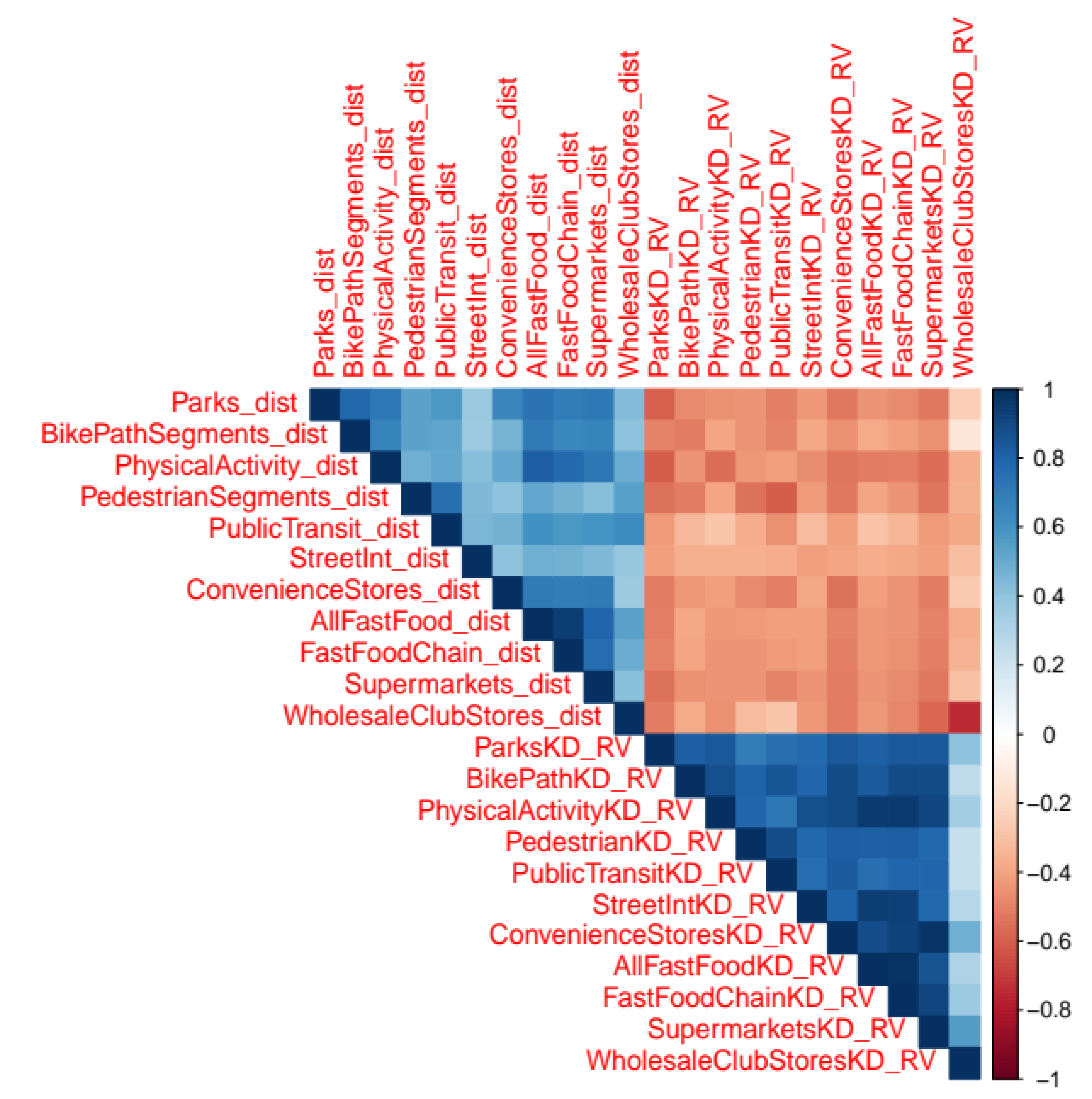
Figure A2.
Correlation heatmap of average raster values for American Community Survey, crime, and satellite data, only while away from home.
Figure A2.
Correlation heatmap of average raster values for American Community Survey, crime, and satellite data, only while away from home.
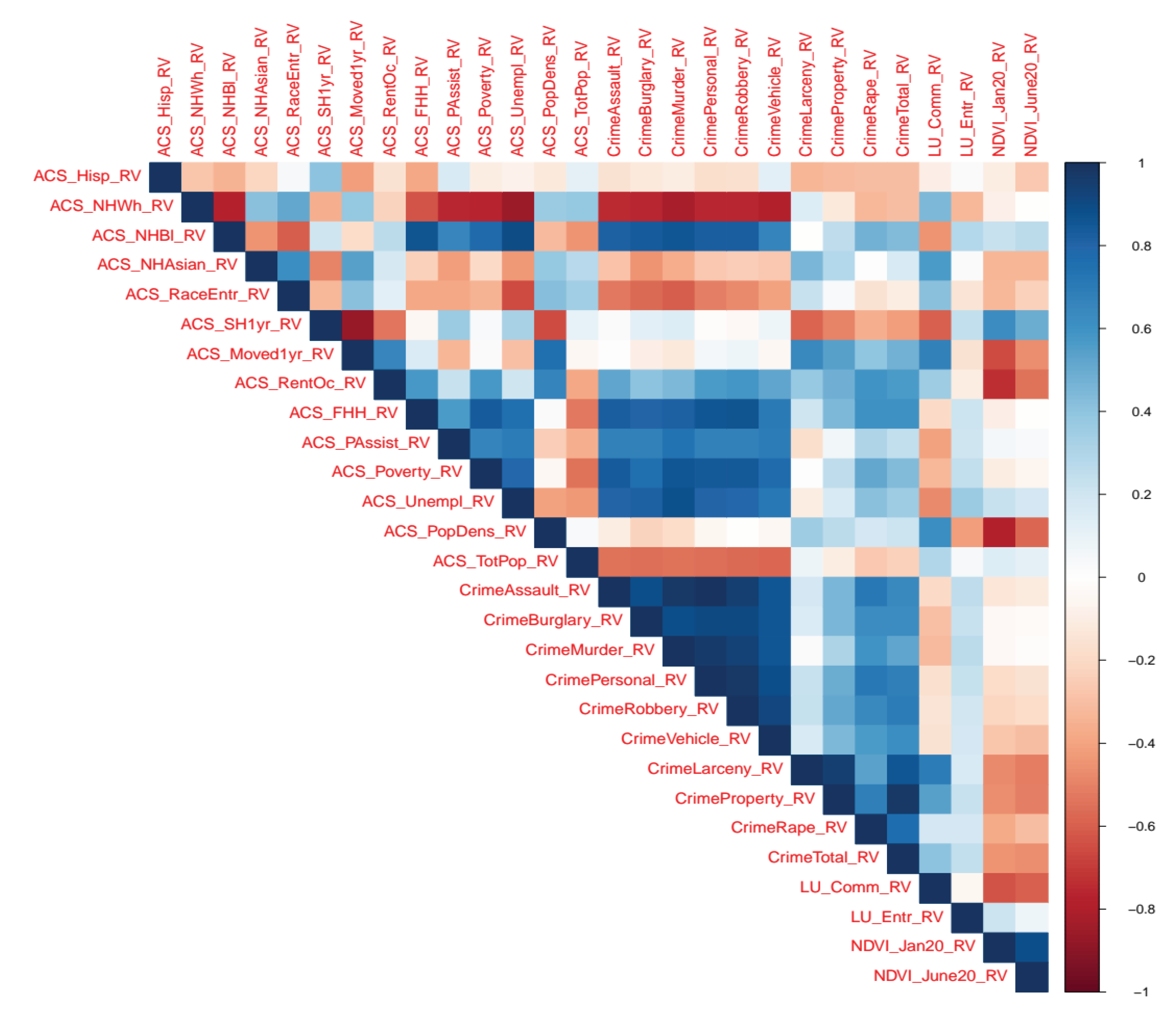

Table A1.
Unadjusted correlations and 95% confidence intervals of average kernel density raster values of location types with participant demographics.
Table A1.
Unadjusted correlations and 95% confidence intervals of average kernel density raster values of location types with participant demographics.
| Location Type (Average Kernel Density) |
Male | Age ≥ 50 | Non-Hispanic Black | Non-Hispanic White | Hispanic |
|---|---|---|---|---|---|
| Public Park | 0.13* (0.02, 0.23) |
-0.10 (-0.21, 0.01) |
-0.31*** (-0.41, -0.21) |
0.30*** (0.19, 0.40) |
0.02 (-0.09, 0.12) |
| Bike Path Segment | 0.13* (0.03, 0.24) |
-0.08 (-0.19, 0.02) |
-0.20*** (-0.30, -0.10) |
0.21*** (0.11, 0.32) |
-0.01 (-0.12, 0.09) |
| Physical Activity Location | 0.16** (0.06, 0.27) |
-0.08 (-0.19, 0.03) |
-0.32*** (-0.42, -0.22) |
0.35*** (0.25, 0.45) |
-0.03 (-0.14, 0.08) |
| Pedestrian Segment | 0.08 (-0.02, 0.19) |
-0.03 (-0.14, 0.07) |
-0.14* (-0.24, -0.03) |
0.08 (-0.03, 0.19) |
0.06 (-0.04, 0.17) |
| Public Transit | 0.09 (-0.02, 0.19) |
-0.01 (-0.12, 0.09) |
-0.07 (-0.18, 0.04) |
0.06 (-0.05, 0.17) |
0.01 (-0.10, 0.12) |
| Street Intersection | 0.08 (-0.03, 0.18) |
-0.10 (-0.21, 0.00) |
-0.20*** (-0.31, -0.10) |
0.19*** (0.08, 0.29) |
0.02 (-0.09, 0.12) |
| Convenience Store | 0.15** (0.05, 0.26) |
-0.14* (-0.24, -0.03) |
-0.40*** (-0.50, -0.31) |
0.26*** (0.16, 0.36) |
0.16** (0.05, 0.26) |
| Any Fast Food Restaurant | 0.14* (0.03, 0.24) |
-0.13* (-0.24, -0.02) |
-0.33*** (-0.43, -0.23) |
0.29*** (0.18, 0.39) |
0.05 (-0.06, 0.16) |
| Fast Food Chain Restaurant | 0.13* (0.03, 0.24) |
-0.14* (-0.24, -0.03) |
-0.36*** (-0.46, -0.26) |
0.27*** (0.16, 0.37) |
0.10 (-0.01, 0.20) |
| Supermarket | 0.14* (0.03, 0.24) |
-0.12* (-0.22, -0.01) |
-0.40*** (-0.50, -0.31) |
0.28*** (0.17, 0.38) |
0.14* (0.03, 0.24) |
| Wholesale Club Store | 0.07 (-0.03, 0.18) |
-0.13* (-0.24, -0.02) |
-0.45*** (-0.55, -0.36) |
0.17** (0.07, 0.28) |
0.30*** (0.20, 0.40) |
Significance indicated by * for p>0.05, ** for p<0.01, *** for p<0.001.
Table A2.
Group means of average kernel density raster values of location types with participant demographics.
Table A2.
Group means of average kernel density raster values of location types with participant demographics.
|
Location Type (Average Kernel Density) |
Male | Female | Age ≥ 50 | Age < 50 | Non-Hispanic Black | Non-Hispanic White | Hispanic |
| Public Park | 4.18 | 3.82 | 3.91 | 4.04 | 3.54 | 4.40 | 3.99 |
| Bike Path Segment | 2.11 | 1.85 | 1.87 | 2.05 | 1.71 | 2.26 | 1.90 |
| Physical Activity Location | 5.92 | 4.90 | 5.10 | 5.58 | 4.01 | 6.79 | 5.17 |
| Pedestrian Segment | 62.42 | 56.83 | 57.35 | 61.23 | 52.02 | 66.71 | 59.06 |
| Public Transit | 51.22 | 47.41 | 48.04 | 50.20 | 46.37 | 52.94 | 47.66 |
| Street Intersection | 513.10 | 489.14 | 491.66 | 508.55 | 460.14 | 542.78 | 496.42 |
| Convenience Store | 5.70 | 5.14 | 5.17 | 5.59 | 4.57 | 6.02 | 5.61 |
| Any Fast Food Restaurant | 15.13 | 13.17 | 13.56 | 14.50 | 11.25 | 16.72 | 14.14 |
| Fast Food Chain Restaurant | 6.33 | 5.68 | 5.76 | 6.17 | 4.98 | 6.82 | 6.12 |
| Supermarket | 1.41 | 1.28 | 1.28 | 1.39 | 1.13 | 1.50 | 1.38 |
| Wholesale Club Store | 0.03 | 0.03 | 0.03 | 0.03 | 0.03 | 0.04 | 0.04 |
Table A3.
Difference of means and 95% confidence intervals of average kernel density raster values of location types by participant demographics including participant time in home buffer.
Table A3.
Difference of means and 95% confidence intervals of average kernel density raster values of location types by participant demographics including participant time in home buffer.
| Location Type (Average Kernel Density) |
Gender1 (Male - Female)1 |
Age (≥50 - <50) |
Non-Hispanic Black (NH Black - NH White) |
Hispanic (Hispanic - NH White) |
|---|---|---|---|---|
| Public Park | 0.381* (0.088, 0.674) |
-0.270 (-0.560, 0.020) |
-1.093*** (-1.407, -0.779) |
-0.494** (-0.858, -0.130) |
| Bike Path Segment | 0.288** (0.071, 0.505) |
-0.168 (-0.382, 0.046) |
-0.547*** (-0.789, -0.304) |
-0.306* (-0.588, -0.024) |
| Physical Activity Location | 1.100** (0.411, 1.790) |
-0.520 (-1.204, 0.164) |
-2.835*** (-3.589, -2.081) |
-1.639*** (-2.495, -0.782) |
| Pedestrian Segment | 5.467 (-0.690, 11.625) |
-1.882 (-8.248, 4.485) |
-8.602* (-16.609, -0.596) |
-0.143 (-7.684, 7.397) |
| Public Transit | 4.029 (-0.391, 8.449) |
-0.520 (-5.030, 3.990) |
-3.580 (-9.312, 2.151) |
-1.300 (-6.490, 3.889) |
| Street Intersection | 26.116 (-5.935, 58.168) |
-31.593 (-64.499, 1.314) |
-79.589*** (-118.243, -40.936) |
-34.234 (-77.056, 8.588) |
| Convenience Store | 0.701** (0.245, 1.157) |
-0.578* (-1.029, -0.126) |
-1.872*** (-2.385, -1.360) |
-0.194 (-0.740, 0.351) |
| Any Fast Food Restaurant | 2.173** (0.660, 3.686) |
-1.859* (-3.386, -0.331) |
-5.869*** (-7.625, -4.113) |
-2.130* (-4.020, -0.240) |
| Fast Food Chain Restaurant | 0.747** (0.190, 1.304) |
-0.720* (-1.278, -0.162) |
-2.160*** (-2.787, -1.533) |
-0.514 (-1.212, 0.185) |
| Supermarket | 0.143** (0.038, 0.249) |
-0.115* (-0.219, -0.011) |
-0.440*** (-0.557, -0.322) |
-0.071 (-0.194, 0.052) |
| Wholesale Club Store | 0.002 (-0.001, 0.005) |
-0.003* (-0.006, -0.001) |
-0.010*** (-0.013, -0.007) |
0.003** (0.001, 0.005) |
*p<0.05; **p<0.01; ***p<0.001. 1Due to the small number of individuals who did not identify as male or female (n=5), they are excluded from the comparison of males to females.
Table A4.
Unadjusted correlations and 95% confidence intervals of average kernel density raster values of location types with average raster values of geographic characteristics from the American Community Survey, EPA walkability, crime reporting, and satellite measurements of land use and vegetative index including participant time in home buffer.
| Location Type (Average Kernel Density) |
ACS Population Density | ACS Poverty | Total Crime | Land Use - Commercial | Normalized Difference Vegetation Index | EPA National Walkability Index |
|---|---|---|---|---|---|---|
| Public Park | 0.59*** (0.50, 0.67) |
-0.09 (-0.20, 0.01) |
0.08 (-0.03, 0.18) |
0.45*** (0.35, 0.54) |
-0.49*** (-0.59, -0.40) |
0.45*** (0.36, 0.55) |
| Bike Path Segment | 0.50*** (0.41, 0.59) |
0.05 (-0.05, 0.16) |
0.31*** (0.21, 0.42) |
0.51*** (0.41, 0.60) |
-0.62*** (-0.71, -0.54) |
0.36*** (0.26, 0.46) |
| Physical Activity Location | 0.51*** (0.41, 0.60) |
-0.31*** (-0.42, -0.21) |
0.11 (0.00, 0.21) |
0.58*** (0.50, 0.67) |
-0.51*** (-0.60, -0.41) |
0.50*** (0.41, 0.59) |
| Pedestrian Segment | 0.53*** (0.44, 0.62) |
0.18*** (0.08, 0.29) |
0.33*** (0.23, 0.43) |
0.37*** (0.27, 0.47) |
-0.67*** (-0.75, -0.59) |
0.31*** (0.21, 0.42) |
| Public Transit | 0.54*** (0.45, 0.63) |
0.33*** (0.23, 0.43) |
0.41*** (0.31, 0.51) |
0.37*** (0.27, 0.47) |
-0.70*** (-0.77, -0.62) |
0.34*** (0.24, 0.44) |
| Street Intersection | 0.44*** (0.35, 0.54) |
-0.10 (-0.21, 0.01) |
0.26*** (0.16, 0.36) |
0.55*** (0.46, 0.64) |
-0.59*** (-0.67, -0.50) |
0.47*** (0.37, 0.56) |
| Convenience Store | 0.56*** (0.48, 0.65) |
-0.20*** (-0.30, -0.10) |
0.09 (-0.02, 0.20) |
0.53*** (0.44, 0.62) |
-0.71*** (-0.78, -0.63) |
0.56*** (0.47, 0.65) |
| Any Fast Food Restaurant | 0.55*** (0.46, 0.64) |
-0.28*** (-0.39, -0.18) |
0.11 (-0.00, 0.21) |
0.60*** (0.52, 0.69) |
-0.58*** (-0.67, -0.49) |
0.50*** (0.40, 0.59) |
| Fast Food Chain Restaurant | 0.53*** (0.44, 0.62) |
-0.25*** (-0.36, -0.15) |
0.13* (0.02, 0.23) |
0.60*** (0.51, 0.68) |
-0.66*** (-0.74, -0.58) |
0.53*** (0.44, 0.62) |
| Supermarket | 0.49*** (0.40, 0.59) |
-0.24*** (-0.35, -0.14) |
0.09 (-0.02, 0.20) |
0.54*** (0.45, 0.63) |
-0.69*** (-0.77, -0.61) |
0.59*** (0.50, 0.68) |
| Wholesale Club Store | 0.16** (0.05, 0.26) |
-0.36*** (-0.46, -0.26) |
-0.21*** (-0.31, -0.10) |
0.19*** (0.08, 0.29) |
-0.39*** (-0.48, -0.29) |
0.49*** (0.40, 0.59) |
*p<0.05; **p<0.01; ***p<0.001.
Table A5.
Statistically significant partial correlations1 of average kernel density raster values for location types with the demographic and geographic variables from Table A3 and Table A4, including participant time spent in home buffer.
| Participant characteristics | Environmental contexts | |||||||||
|---|---|---|---|---|---|---|---|---|---|---|
| Activity Space (kd) |
Male | Age ≥ 50 | NH Black | Hispanic | ACS Pop. Density | ACS Poverty | Total Crime | Land Use Com. | NDVI | EPA NWI |
| Public Park | -0.23 *** |
-0.14 * |
0.43 *** |
0.19 *** |
0.25 *** |
|||||
| Bike Path Segment | -0.22 *** |
-0.18 *** |
0.25 *** |
0.34 *** |
0.21 *** |
-0.29 *** |
0.21 *** |
|||
| Physical Activity Location | -0.24 *** |
-0.20 *** |
0.39 *** |
-0.45 *** |
0.41 *** |
0.22 *** |
0.21 *** |
|||
| Pedestrian Segment | -0.12 * |
0.29 *** |
0.26 *** |
-0.37 *** |
||||||
| Public Transit | 0.11 * |
-0.13 * |
0.29 *** |
0.24 *** |
0.23 *** |
-0.42 *** |
0.17 ** |
|||
| Street Intersection | -0.11 * |
0.21 *** |
-0.23 *** |
0.33 *** |
0.23 *** |
-0.23 *** |
0.17 ** |
|||
| Convenience Store | -0.26 *** |
0.34 *** |
-0.32 *** |
0.28 *** |
-0.41 *** |
0.25 *** |
||||
| Any Fast Food Restaurant | -0.18 *** |
0.40 *** |
-0.43 *** |
0.38 *** |
0.22 *** |
-0.20 *** |
0.18 ** |
|||
| Fast Food Chain Restaurant | -0.21 *** |
0.33 *** |
-0.42 *** |
0.37 *** |
0.19 *** |
-0.35 *** |
0.19 *** |
|||
| Supermarket | -0.27 *** |
0.23 *** |
-0.36 *** |
0.29 *** |
-0.42 *** |
0.29 *** |
||||
| Wholesale Club Store | -0.17 ** |
-0.24 *** |
-0.17 ** |
-0.28 *** |
0.31 *** |
|||||
*p<0.05; **p<0.01; ***p<0.001. Each partial correlation was estimated while controlling for all other demographic and geographic variables.
References
- Hales CM, Carroll MD, Fryar CD, Ogden CL: Prevalence of Obesity Among Adults and Youth: United States, 2015-2016. NCHS Data Brief 2017:1-8.
- MA F, K S, D N, X Y, LB S, RJ M, RB M, R W, A H, A B, et al: Sugar-sweetened beverage intake and cancer recurrence and survival in CALGB 89803 (Alliance) - PubMed. PloS one 06/17/2014, 9.
- SC M, IM L, E W, PT C, JN S, CM K, SK K, H A, A BdG, P H, et al: Association of Leisure-Time Physical Activity With Risk of 26 Types of Cancer in 1.44 Million Adults - PubMed. JAMA internal medicine 06/01/2016, 176.
- LR P, H N, DM L-J, NB A: Trends in Racial/Ethnic Disparities in Cardiovascular Health Among US Adults From 1999-2012 - PubMed. Journal of the American Heart Association 09/22/2017, 6.
- K PG, B S, A C, A S, ES S, JA C, S D, C K-G: Physical activity trajectories during midlife and subsequent risk of physical functioning decline in late mid-life: The Study of Women's Health Across the Nation (SWAN) - PubMed. Preventive medicine 2017 Dec, 105.
- Lachman ME, Teshale S, Agrigoroaei S: Midlife as a Pivotal Period in the Life Course: Balancing Growth and Decline at the Crossroads of Youth and Old Age. International journal of behavioral development 2014 May 14, 39.
- Available online: https://www.cdc.gov/about/priorities/why-is-addressing-sdoh-important.html.
- M K, T L, T I, H K-H, R K: The Built Environment as a Determinant of Physical Activity: A Systematic Review of Longitudinal Studies and Natural Experiments - PubMed. Annals of behavioral medicine : a publication of the Society of Behavioral Medicine 02/17/2018, 52.
- C P, B C, S C, Y K: Conceptualization and measurement of environmental exposure in epidemiology: accounting for activity space related to daily mobility - PubMed. Health & place 2013 May, 21.
- Bronas UG, Kershaw KN, Tu J, Ryder N, Westra J, Redondo-Sáenz D, Tintle N: Frontiers | Everyday Environmental Exposures and Mid-Life Dietary and Physical Activity Variations: E3 Study Protocol. Frontiers in Public Health, 13.
- Tintle N, Tu J, Luong A, Min S, Kershaw KN, Bronas UG: Semi-Automated Processing of Harmonized Accelerometer and GPS Data in R: AGPSR. Sensors (Basel, Switzerland) 2025 Jun 22, 25.
- Silverman B: Density estimation for statistics and data analysis.; Chapman and Hall: New York, New York, USA, 1986.
- Carr LJ, Dunsiger SI, Marcus BH: Walk Score™ As a Global Estimate of Neighborhood Walkability. American journal of preventive medicine 2010 Nov, 39.
- Agurs-Collins T, Alvidrez J, Ferreira SE, Evans M, Gibbs K, Kowtha B, Pratt C, Reedy J, Shams-White M, Brown AG: Perspective: Nutrition Health Disparities Framework: A Model to Advance Health Equity. Advances in Nutrition 2024/04/01, 15.
- McCullough ML, Chantaprasopsuk S, Islami F, Rees-Punia E, Um CY, Wang Y, Leach CR, Sullivan KR, Patel AV: Association of Socioeconomic and Geographic Factors With Diet Quality in US Adults. JAMA Network Open 2022/06/01, 5.
- Schertz KE, Saxon J, Cardenas-Iniguez C, Bettencourt LMA, Ding Y, Hoffmann H, Berman MG, Schertz KE, Saxon J, Cardenas-Iniguez C, et al: Neighborhood street activity and greenspace usage uniquely contribute to predicting crime. npj Urban Sustainability 2021 1:1 2021-04-27, 1.
- Schusler T, Weiss L, Treering D, Balderama E: Research note: Examining the association between tree canopy, parks and crime in Chicago. Landscape and Urban Planning 2018/02/01, 170. Landscape and Urban Planning.
- Groff E, McCord ES, Groff E, McCord ES: The role of neighborhood parks as crime generators. Security Journal 2011 25:1 2011-03-07, 25.
- Askey AP, Taylor R, Groff E, Fingerhut A, Amber Perenzin Askey RT, Elizabeth Groff,Aaron Fingerhut: Fast Food Restaurants and Convenience Stores: Using Sales Volume to Explain Crime Patterns in Seattle. Crime & Delinquency 2018-12, 64.
- Wolfe SE, Pyrooz DC: Rolling Back Prices and Raising Crime Rates? The Walmart Effect on Crime in the United States. The British Journal of Criminology 2014/03/01, 54.
- Singleton CR, Winata F, Adams AM, McLafferty SL, Sheehan KM, Zenk SN: County-level associations between food retailer availability and violent crime rate. BMC Public Health 2022 Nov 1, 22.
- SN Z, SA M, AN K, KK J: How many days of global positioning system (GPS) monitoring do you need to measure activity space environments in health research? - PubMed. Health & place 2018 May, 51.
Figure 1.
CONSORT diagram.
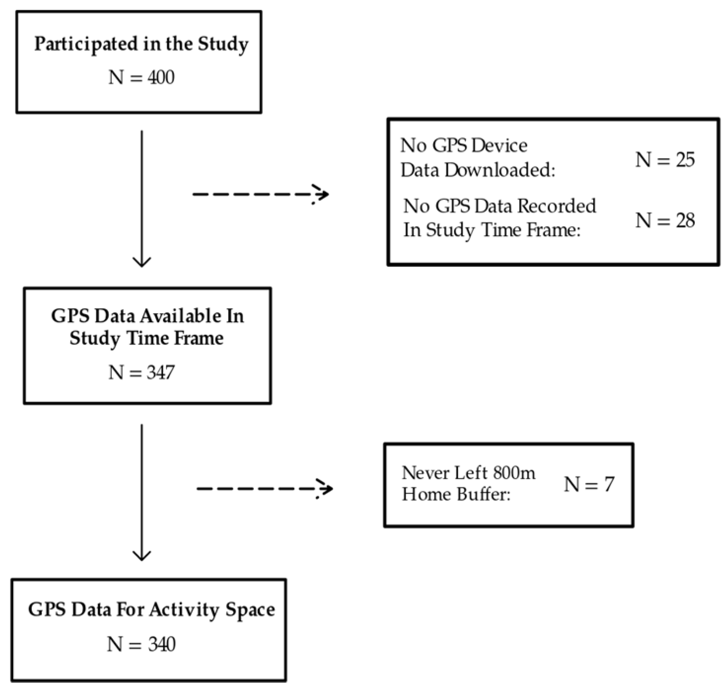
Figure 2.
Example computation of kernel density for convenience stores.
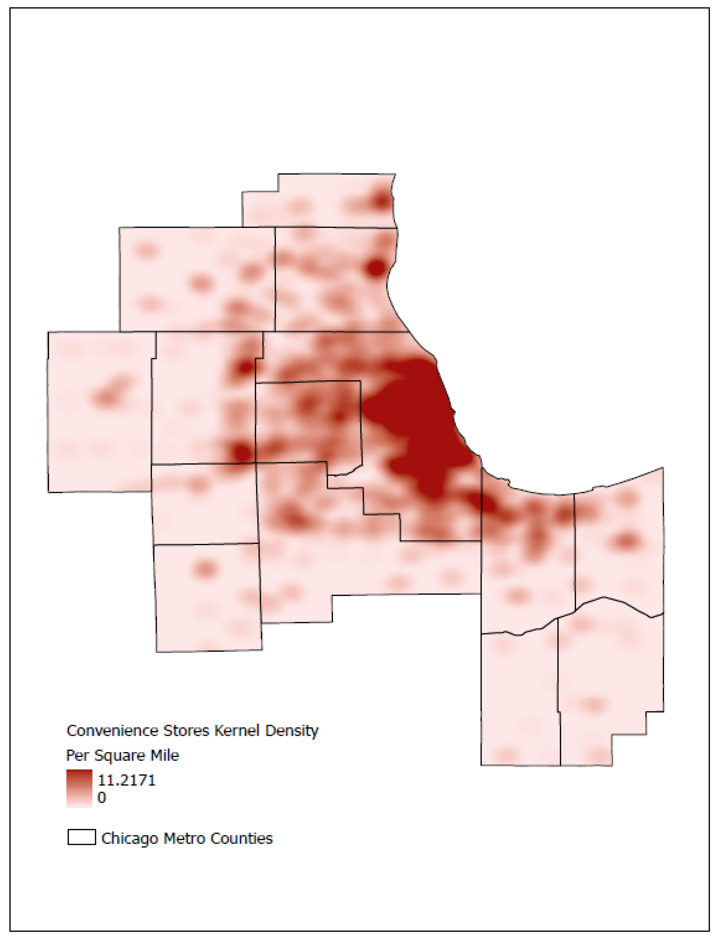
Table 1.
Participant characteristics (N=340).
| Characteristics | Count (%) or mean ± SD |
|---|---|
| Gender | |
| Man | 135 (39.7) |
| Woman | 200 (58.8) |
| Transgender or Non-Binary | 5 (1.5) |
| Age | 50.4 ± 7.3 |
| Race/Ethnicity | |
| Non-Hispanic White | 123 (36.2) |
| Non-Hispanic Black | 124 (36.5) |
| Hispanic | 93 (27.4) |
| Education | |
| Less Than High School | 13 (3.8) |
| High School | 93 (27.4) |
| College - 2 to 4 years | 124 (36.5) |
| College - 5+ years | 110 (32.4) |
| Marital Status | |
| Never Married | 115 (33.8) |
| Married | 133 (39.1) |
| Divorced/Separated | 85 (25.0) |
| Widowed | 5 (1.5) |
| Income | |
| < 50,000 | 95 (27.9) |
| 50 - 150,000 | 126 (37.1) |
| > 150,000 | 75 (22.1) |
| No Answer | 44 (12.9) |
| BMI | 29.9 ± 7.2 |
| Missing | 3 (0.9) |
| Walk Score | 75.0 ± 17.3 |
Table 2.
GPS measured points summary statistics (n=340).
| Including Minutes Spent In Home Buffer | Measure | Minimum | Mean ± SD | Maximum |
|---|---|---|---|---|
| Yes | Total GPS Points (Minutes) | 529 | 21,146.2 ± 7543.1 | 29,744 |
| Number of Days GPS Was Used | 2 | 18.4 ± 4.6 | 21 | |
| No | Total GPS Points (Minutes) | 28 | 4,173.8 ± 4,246.9 | 27,379 |
| Number of Days GPS Was Used | 1 | 14.4 ± 5.2 | 21 |
Table 3.
Summary statistics for average closest distances and average kernel density raster values for various location types across all participants (N=340)1.
Table 3.
Summary statistics for average closest distances and average kernel density raster values for various location types across all participants (N=340)1.
| Location Type | Minimum | Mean ± SD | Maximum |
|---|---|---|---|
| Average Closest Distance in Meters | |||
| Public Park | 131.5 | 469.7 ± 257.4 | 3553.9 |
| Bike Path Segment | 34.2 | 690.8 ± 786.5 | 12585.5 |
| Physical Activity Location | 89.5 | 492.4 ± 300.2 | 3730.1 |
| Pedestrian Segment | 9.7 | 167.1 ± 254.3 | 3105.5 |
| Public Transit | 26.7 | 344.7 ± 617.1 | 6493.0 |
| Street Intersection | 16.3 | 41.9 ± 15.6 | 121.6 |
| Convenience Store | 88.7 | 385.5 ± 205.3 | 1424.5 |
| Any Fast Food Restaurant | 78.3 | 319.9 ± 236.7 | 3165.5 |
| Fast Food Chain Restaurant | 107.4 | 412.4 ± 270.2 | 3292.6 |
| Supermarket | 186.1 | 684.2 ± 338.1 | 4228.3 |
| Wholesale Club Store | 1297.8 | 3885.6 ± 2012.2 | 21782.7 |
| Average Kernel Density (Per Square Mile) Raster Value | |||
| Public Park | 0.7 | 4.0 ± 1.2 | 6.5 |
| Bike Path Segment | 0.1 | 2.0 ± 0.9 | 3.9 |
| Physical Activity Location | 0.4 | 5.3 ± 3.2 | 14.5 |
| Pedestrian Segment | 0.6 | 59.3 ± 29.4 | 170.2 |
| Public Transit | 0.8 | 49.1 ± 20.6 | 114.5 |
| Street Intersection | 112.3 | 500.0 ± 179.6 | 1258.7 |
| Convenience Store | 1.0 | 5.4 ± 2.0 | 9.7 |
| Any Fast Food Restaurant | 1.1 | 14.0 ± 7.8 | 42.0 |
| Fast Food Chain Restaurant | 0.7 | 6.0 ± 2.8 | 14.4 |
| Supermarket | 0.2 | 1.3 ± 0.5 | 2.4 |
| Wholesale Club Store | 0.0 | 0.0 ± 0.0 | 0.1 |
1All activity space measures for each participant were first averaged across all minute-level measurements in the 21-day study period, not including minutes when they were at home.
Table 4.
Summary statistics for activity space raster values across all participants (N=340)1.
| Variable (Raster Value) | Minimum | Mean ± SD | Maximum |
|---|---|---|---|
| ACS Hispanic (%) | 2.6 | 21.3 ± 13.5 | 87.0 |
| ACS Non-Hispanic White (%) | 2.0 | 44.8 ± 17.8 | 82.1 |
| ACS Non-Hispanic Black (%) | 1.4 | 21.8 ± 20.9 | 91.6 |
| ACS Non-Hispanic Asian (%) | 0.2 | 8.7 ± 4.5 | 22.8 |
| ACS Race Entropy | 0.2 | 0.6 ± 0.1 | 0.8 |
| ACS Female-Headed Households (%) | 21.5 | 37.1 ± 7.2 | 69.5 |
| ACS Renter Occupied (%) | 9.7 | 50.0 ± 12.0 | 75.8 |
| ACS Same House as 1 Year Ago (%) | 59.9 | 82.9 ± 5.3 | 93.1 |
| ACS Moved within 1 Year (%) | 6.0 | 16.6 ± 5.1 | 30.8 |
| ACS Public Assistance (%) | 0.8 | 2.6 ± 1.1 | 7.6 |
| ACS Poverty (%) | 4.8 | 14.8 ± 6.3 | 42.7 |
| ACS Unemployment (%) | 1.2 | 4.5 ± 2.0 | 12.2 |
| ACS Population Density (number of people per sq km) | 2941.9 | 18471.4 ± 8740.8 | 46134.6 |
| ACS Total Population (number of people) | 1337.6 | 3927.7 ± 742.8 | 7773.2 |
| EPA National Walkability Index | 6.7 | 14.7 ± 1.3 | 17.2 |
| Crime Burglary (events/year) | 20.5 | 101.3 ± 40.2 | 271.7 |
| Crime Murder (events/year) | 13.3 | 211.5 ± 161.6 | 966.0 |
| Crime Personal (events/year) | 19.7 | 162.6 ± 85.5 | 551.4 |
| Crime Robbery (events/year) | 22.1 | 248.7 ± 124.3 | 794.4 |
| Crime Vehicle (events/year) | 16.7 | 134.9 ± 53.0 | 321.3 |
| Crime Larceny (events/year) | 43.8 | 153.8 ± 49.4 | 354.1 |
| Crime Property (events/year) | 40.4 | 141.2 ± 38.9 | 282.8 |
| Crime Rape (events/year) | 24.7 | 117.3 ± 43.3 | 291.3 |
| Total Crime (events/year) | 37.6 | 144.0 ± 40.5 | 270.3 |
| Land Use - Commercial | 0.0 | 0.1 ± 0.0 | 0.3 |
| Land Use - Entropy | 0.3 | 0.4 ± 0.0 | 0.6 |
| Normalized Difference Vegetation Index, Jan '20 | 0.1 | 0.2 ± 0.0 | 0.3 |
| Normalized Difference Vegetation Index, June '20 | 0.2 | 0.3 ± 0.1 | 0.6 |
1All activity space measures for each participant were first averaged across all minute-level measurements in the 21-day study period, not including minutes when they were at home. .
Table 5.
Difference of means and 95% confidence intervals of average kernel density raster values of location types by participant demographics. 1.
Table 5.
Difference of means and 95% confidence intervals of average kernel density raster values of location types by participant demographics. 1.
| Location Type (Average Kernel Density) |
Gender1 (Male - Female)1 |
Age (≥50 - <50) |
Non-Hispanic Black (NH Black - NH White) |
Hispanic (Hispanic - NH White) |
|---|---|---|---|---|
| Public Park | 0.365** (0.103, 0.626) |
-0.132 (-0.392, 0.127) |
-0.861*** (-1.160, -0.562) |
-0.414** (-0.720, -0.108) |
| Bike Path Segment | 0.252* (0.050, 0.455) |
-0.180 (-0.378, 0.019) |
-0.543*** (-0.774, -0.313) |
-0.351** (-0.597, -0.104) |
| Physical Activity Location | 1.027** (0.329, 1.726) |
-0.483 (-1.168, 0.202) |
-2.778*** (-3.545, -2.011) |
-1.619*** (-2.439, -0.800) |
| Pedestrian Segment | 5.586 (-0.772, 11.944) |
-3.881 (-10.128, 2.366) |
-14.691*** (-22.144, -7.238) |
-7.653 (-15.354, 0.047) |
| Public Transit | 3.813 (-0.628, 8.254) |
-2.161 (-6.555, 2.233) |
-6.568* (-11.927, -1.210) |
-5.282 (-10.596, 0.032) |
| Street Intersection | 23.957 (-15.398, 63.312) |
-16.889 (-55.146, 21.367) |
-82.646*** (-127.761, -37.531) |
-46.357 (-93.543, 0.829) |
| Convenience Store | 0.563* (0.132, 0.994) |
-0.426* (-0.849, -0.004) |
-1.449*** (-1.947, -0.950) |
-0.409 (-0.912, 0.094) |
| Any Fast Food Restaurant | 1.961* (0.244, 3.678) |
-0.940 (-2.612, 0.732) |
-5.468*** (-7.417, -3.519) |
-2.573* (-4.558, -0.587) |
| Fast Food Chain Restaurant | 0.649* (0.049, 1.249) |
-0.409 (-0.996, 0.177) |
-1.837*** (-2.524, -1.149) |
-0.698* (-1.393, -0.002) |
| Supermarket | 0.126* (0.026, 0.226) |
-0.108* (-0.206, -0.010) |
-0.373*** (-0.488, -0.258) |
-0.117* (-0.232, -0.003) |
| Wholesale Club Store | 0.002 (-0.000, 0.004) |
-0.002* (-0.004, -0.000) |
-0.006*** (-0.008, -0.003) |
0.002* (0.001, 0.004) |
*p<0.05; **p<0.01; ***p<0.001. 1Due to the small number of individuals who did not identify as male or female (n=5), they are excluded from the comparison of males to females.
Table 6.
Unadjusted correlations and 95% confidence intervals of average kernel density raster values of location types with average raster values of geographic characteristics from the American Community Survey, EPA walkability, crime reporting, and satellite measurements of land use and vegetative index.
| Location Type (Average Kernel Density) |
ACS Population Density | ACS Poverty | Total Crime | Land Use - Commercial | Normalized Difference Vegetation Index | EPA National Walkability Index |
|---|---|---|---|---|---|---|
| Public Park | 0.76*** (0.69, 0.83) |
-0.06 (-0.17, 0.04) |
0.40*** (0.30, 0.50) |
0.67*** (0.59, 0.75) |
-0.64*** (-0.72, -0.56) |
0.74*** (0.66, 0.81) |
| Bike Path Segment | 0.68*** (0.60, 0.76) |
0.04 (-0.06, 0.15) |
0.55*** (0.46, 0.64) |
0.64*** (0.56, 0.73) |
-0.71*** (-0.78, -0.63) |
0.63*** (0.54, 0.71) |
| Physical Activity Location | 0.72*** (0.65, 0.79) |
-0.31*** (-0.41, -0.21) |
0.42*** (0.32, 0.51) |
0.78*** (0.71, 0.84) |
-0.65*** (-0.73, -0.57) |
0.69*** (0.61, 0.76) |
| Pedestrian Segment | 0.77*** (0.70, 0.84) |
0.03 (-0.08, 0.14) |
0.50*** (0.40, 0.59) |
0.66*** (0.58, 0.74) |
-0.69*** (-0.77, -0.61) |
0.59*** (0.50, 0.68) |
| Public Transit | 0.75*** (0.68, 0.82) |
0.24*** (0.14, 0.35) |
0.63*** (0.54, 0.71) |
0.64*** (0.56, 0.72) |
-0.74*** (-0.81, -0.66) |
0.63*** (0.55, 0.71) |
| Street Intersection | 0.58*** (0.50, 0.67) |
-0.12* (-0.23, -0.02) |
0.62*** (0.53, 0.70) |
0.81*** (0.75, 0.88) |
-0.70*** (-0.78, -0.62) |
0.66*** (0.57, 0.74) |
| Convenience Store | 0.75*** (0.67, 0.82) |
-0.15** (-0.26, -0.05) |
0.44*** (0.34, 0.53) |
0.72*** (0.64, 0.79) |
-0.77*** (-0.84, -0.70) |
0.77*** (0.70, 0.84) |
| Any Fast Food Restaurant | 0.71*** (0.63, 0.78) |
-0.26*** (-0.36, -0.15) |
0.49*** (0.40, 0.58) |
0.83*** (0.77, 0.89) |
-0.70*** (-0.78, -0.63) |
0.68*** (0.60, 0.76) |
| Fast Food Chain Restaurant | 0.70*** (0.62, 0.77) |
-0.19*** (-0.30, -0.09) |
0.52*** (0.43, 0.61) |
0.79*** (0.73, 0.86) |
-0.76*** (-0.83, -0.69) |
0.72*** (0.65, 0.79) |
| Supermarket | 0.70*** (0.63, 0.78) |
-0.19*** (-0.29, -0.09) |
0.40*** (0.30, 0.50) |
0.68*** (0.61, 0.76) |
-0.77*** (-0.84, -0.70) |
0.79*** (0.72, 0.85) |
| Wholesale Club Store | 0.24*** (0.13, 0.34) |
-0.32*** (-0.42, -0.22) |
-0.07 (-0.17, 0.04) |
0.29*** (0.19, 0.39) |
-0.48*** (-0.58, -0.39) |
0.56*** (0.47, 0.64) |
*p<0.05; **p<0.01; ***p<0.001.
Table 7.
Statistically significant partial correlations1 of average kernel density raster values for location types with the demographic and geographic variables from Table 5 and Table 6.
| Participant characteristics | Environmental contexts | |||||||||
|---|---|---|---|---|---|---|---|---|---|---|
| Activity Space (kd) |
Male | Age ≥ 50 | NH Black | Hispanic | ACS Pop. Density | ACS Poverty | Total Crime | Land Use Com. | NDVI | EPA NWI |
| Public Park | -0.18 ** |
-0.11 * |
0.50 *** |
0.22 *** |
0.44 *** |
|||||
| Bike Path Segment | -0.26 *** |
-0.19 *** |
0.39 *** |
0.38 *** |
-0.28 *** |
|||||
| Physical Activity Location | -0.23 *** |
-0.22 *** |
0.57 *** |
-0.54 *** |
0.51 *** |
-0.21 *** |
0.20 *** |
|||
| Pedestrian Segment | -0.13 * |
0.60 *** |
0.36 *** |
-0.24 *** |
||||||
| Public Transit | -0.18 *** |
-0.12 * |
0.59 *** |
0.35 *** |
0.39 *** |
0.19 *** |
-0.27 *** |
0.19 *** |
||
| Street Intersection | 0.17 ** |
-0.25 *** |
0.51 *** |
0.39 *** |
-0.24 *** |
0.15 ** |
||||
| Convenience Store | -0.21 *** |
0.53 *** |
-0.32 *** |
0.39 *** |
-0.38 *** |
0.38 *** |
||||
| Any Fast Food Restaurant | -0.13 * |
0.52 *** |
-0.50 *** |
0.53 *** |
0.26 *** |
-0.29 *** |
||||
| Fast Food Chain Restaurant | -0.18 *** |
0.46 *** |
-0.42 *** |
0.52 *** |
0.15 ** |
-0.39 *** |
0.20 *** |
|||
| Supermarket | -0.27 *** |
-0.18 ** |
0.44 *** |
-0.35 *** |
0.35 *** |
-0.14 * |
-0.43 *** |
0.42 *** |
||
| Wholesale Club Store | -0.17 ** |
-0.19 *** |
-0.17 ** |
-0.37 *** |
0.36 *** |
|||||
*p<0.05; **p<0.01; ***p<0.001. Each partial correlation was estimated while controlling for all other demographic and geographic variables.
Disclaimer/Publisher’s Note: The statements, opinions and data contained in all publications are solely those of the individual author(s) and contributor(s) and not of MDPI and/or the editor(s). MDPI and/or the editor(s) disclaim responsibility for any injury to people or property resulting from any ideas, methods, instructions or products referred to in the content. |
© 2026 by the authors. Licensee MDPI, Basel, Switzerland. This article is an open access article distributed under the terms and conditions of the Creative Commons Attribution (CC BY) license (http://creativecommons.org/licenses/by/4.0/).
Copyright: This open access article is published under a Creative Commons CC BY 4.0 license, which permit the free download, distribution, and reuse, provided that the author and preprint are cited in any reuse.


