Effects of the Spatial Distribution of Activities and Gender Issues in Travel Behavior in the Barcelona Metropolitan Region

Lídia Montero; Lucía Mejía-Dorantes; Jaume Barceló

doi:10.20944/preprints202409.0706.v1

Submitted:

09 September 2024

Posted:

10 September 2024

You are already at the latest version

Abstract

Transport systems are essential in the path towards sustainable urbanisation and the transition to more sustainable living. Recently, European cities have undergone substantial changes, owing to which suburbanisation is posing new challenges. Suburban areas are often more affordable in terms of housing, but their neighbourhoods tend to be car-oriented. This leads to higher commuter costs, immobility, transport and time poverty, pollution, and accident rates and a lack of social interaction. To offer sustainable mobility options to citizens, we must comprehensively understand their specific mobility practices, together with their personal characteristics, and the built environment. This study centred on the Barcelona Metropolitan Region, which has a public transport network that covers the entire area. The aim of this study was to examine the relationship between travel behaviour, transport mode use, individual characteristics, and place of residence, using detailed information sources. Herein, we used data from the annual travel survey conducted in the Barcelona region from 2018 to 2021, together with land-use and other information sources. Our findings suggest that transport policies have encouraged sustainable mobility practices, particularly in the centre of Barcelona. Despite the positive results, considerable disparities exist between the inner and outer city, with notably decreased sustainable mobility practices in the latter. Our results indicate that promoting sustainable mobility policies requires further changes in transport, city, and land-use planning that consider equity, the socioeconomic profile of citizens, and mixed urban planning.

Keywords:

travel behaviour

;

sequence analysis

;

equity

;

clustering

;

spatial analysis

;

gender

Subject:

Social Sciences - Urban Studies and Planning

1. Introduction

The right to the city, a term first proposed by Henri Lefebvre in 1968 [1], has evolved into a concept that seeks inclusivity, accessibility, and democracy in urban spaces. Urbanisation poses major challenges, as most of the world’s population will live in cities by 2050. Therefore, the 2030 Sustainable Development Agenda and the New Urban Agenda [2], call for the promotion of sustainable urbanisation.

On the path to sustainable urbanisation and the transition to a more sustainable living in cities, transport systems are an essential component. Transport is crucial for exercising our right to the city, by facilitating our daily activities and influencing our quality of life. Transport enables us to commute, work, learn, produce, buy and sell, gather information, meet our energy needs, and participate in cultural, health, and social activities. The built environment together with technological innovation also shape our transport systems. Additionally, micro-mobility alternatives and transport on demand (MaaS) have transformed urban spaces and influence the way we move.

However, the transport systems and the built environment are not the only factors that shape our mobility: our personal characteristics, including age, gender, origin, religion, disability, and income, influence how we move, conditioned also by the connectivity of the transport system, the modal choices it offers and their accessibility.

In Europe, cities have evolved, and suburbanisation is posing new challenges. Poverty is moving out of the city centre and “decentralising” to the city outskirts, as a result not only of increasing population but also of income inequalities, lack of social housing combined with market-oriented housing policies, gentrification, and urban segregation [3,4,5]. Car-oriented neighbourhoods pose different challenges in terms of higher commuter costs, immobility, transport and time poverty, pollution, accident rates, and lack of social interaction [6].

The recent breakthrough achieved with 15, 20, or X-minute cities highlight the idea that mixed-land-use neighbourhoods provide citizens with convenient opportunities, easing the access to the activities while substantially reducing the number of unnecessary trips to foster their sustainable mobility, which positively impact citizens’ well-being. However, important disparities remain in service provision, land-use planning, and transport alternatives among neighbourhoods [7,8].

For these reasons, the opportunities that transport systems, especially sustainable transport systems, provide to the population must be analysed in detail according to their different individual socioeconomic characteristics.

In the case of the Metropolitan Region of Barcelona (RMB), the results of previous analyses [9] showed that the socioeconomic characteristics of citizens, education level, age, gender, the built environment, and accessibility to public transport play a large role in shaping mobility. To date, studies on these individual, socioeconomic, and spatial dependencies have only considered wide areas within the RMB such as those shown in Figure 1. Therefore, a more detailed analysis using finer-scale spatial units is necessary. The traffic analysis zone (TAZ), commonly used in transportation analysis, opens up new opportunities, providing additional information for official travel surveys, such as information on socioeconomic status, land use, accessibility, and urban form.

The remainder of this paper is structured as follows: Section 2 defines the objectives of the paper, Section 3 is the literature review, Section 4 presents the case study and its characteristics. Section 5 describes the data sources to define variables, as well as their calculation. Section 6 introduces and describes the methodological approach on which the study was based for the base and full analyses. Section 7 presents the results of the analyses. Finally, Section 8 draws the main conclusions and the final discussion.

2. Objectives

In Barcelona, the analysis of the 2018, 2019, 2020, and 2021 travel surveys from the Metropolitan Transport Authorities in Barcelona (commonly known as EMEF travel surveys), constituted a preliminary analysis of the spatial effects in travel behaviour [9,10], exploring the connection between the declared modal use frequencies (generic modal preferences), individual characteristics, and place of residence. The results showed high levels of public transport use, together with limited car use, by residents of Barcelona city (BCN). In contrast, frequent car use and non-active modes were found in the outer Barcelona metropolitan region (RMB).

The clear spatial dependencies between individual characteristics, transport mode use, and residence areas (including gender, land use, and built environment indicators, as well as indicators related to the sequences of activities of trip-makers) motivates this study with the aim of gaining a deeper insight into these dependencies. Therefore, the aim of this paper is to apply the methodology of sequence analysis (SA) to EMEF datasets combined with land-use, built-environment, accessibility, and other socioeconomic data to gain further insights into mobility behaviour depending on several factors including gender, education, economic level, among others, and their spatial distribution in the RMB.

We are sure that the insights gained from this analysis will contribute to the future development of an activity-based demand model for the RMB. As evidenced by authors such as [11] travel surveys, as exemplified by the one used in this study (EMEF), are a primary requirement for developing activity-based travel demand models that order activities and trips across time and space. These models may be further enhanced through the incorporation of supplementary data sources. Such models may serve as the foundation for tailored transport policies.

3. Literature Review

Many studies in travel behaviour have highlighted the connection between the modal use frequencies, individual characteristics, and place of residence [9,12], however, studies using sequence analysis to account for fragmentation indicators together with land use characteristics are relatively limited as [NO_PRINTED_FORM] [13] observed. The former limits land use and transport policy recommendations.

Sequence analysis (SA) aims at understanding the occurrence of activities or events in a structured way. A sequence is defined a s a list of events and actions performed in an ordered manner. Many authors have developed these concepts and methodologies over the years [14,15,16,17,18]. As observed by McBride et al. [19] analysing sequences of daily episodes (including places and trips) is an approach that may be considered preferable over other techniques as the sequences include the entire trajectory of an individual’s activity thorough a day, while at the same time, it is possible to evaluate the number and order of activities, together with their duration.

Studer and Ritschard [20] identify a number of key characteristics that are inextricably linked: experienced states, distribution, timing, duration and sequencing. Sequence analysis has proven to be a relevant approach to travel behaviour analysis as it describes fragmentation of activities and daily patterns in terms of a string of activities and transitions from one state to the other, which includes the amount of time spent in each activity and trip details [13].

Whereas, many indicators may be used to represent state sequences [21], only a subset of these is relevant to travel behaviour analyses. The most applicable and extensively used indicators within this domain are entropy, turbulence, complexity, and travel time ratio [22,23,24]. These indicators facilitate the analysis and measurement of activity durations and transition rates among them, offering insights into the diversity and intricacy of sequences. Here, an activity sequence comprises a list of states specifying the activity/state applicable for every minute in a day [25] Different sequence analyses have been recently conducted in travel behaviour studies [13,26,27]. In the Appendix, Table A2 provides the main details of the different indicators used in this study, together with the relevant references.

On the other hand, clustering analysis has been used many times to group observations based on different parameters. It is a fundamental exploratory technic in Data Mining. Its goal is to highlight certain similarities and dissimilarities among observations in a dataset to unveil a set of categories, which become the main groups of interest and the object of study [28,29].

Different studies the field of transport behaviour have used this approach to analyse population similarities or differences. For example McBride et al. [19] who cluster representative daily behaviour patterns and Shi et al. [13] who analysed groups of observations with similarly high or low fragmentation. Furthermore, von Behren et al. [30] who carried out an image-based clustering analysis of the individuals’ pattern segmentation using the German Mobility Panel.

4. Barcelona Metropolitan Region (RMB) Case Study

The Barcelona Metropolitan Region (RMB) is used as a case study which is depicted in Figure 1. The RMB, with more than 5 million inhabitants, covering 3200 km², and including 164 municipalities, is connected by a dense public transport network including more than 200 bus lines, 4000 bus-stops, 10 metro lines, 15 train lines, and 2 tram lines. During a working day, approximately 17,5 million trips are made in the RMB.

Figure 1 presents the main areas into which the RMB is divided. The city of Barcelona (BCN) is divided into 10 districts (highlighted in red), the primary crown of the RMB (in orange), the rest of the Barcelona metropolitan area (AMB) (in light green), and the rest of the metropolitan region (in turquoise).

The information from [31] shows differences on mobility by activity purpose: mandatory and discretionary mobility account for 39.8% of the trips, whereas mobility for working purposes account for 17.5% of the daily travel patterns. The rest of the trips are those back home (42.7%).

On the other hand, mobility by private vehicles increases as the area of residence moves away from Barcelona city, whereas active mobility and public transport use decreases. Residents in the Barcelona municipality use public transport in 24% of their journeys, while residents in the rest of the RMB use it in 8.7% of their trips during weekdays. It is worth noting that in the case of trips within the Barcelona Municipality and those carried out between Barcelona with the rest of the primary crown (ETM), there are more trips in public than private transport, with a 180/100 ratio and 117/100, respectively.

It is worth noting that Figure 1 also shows the boundaries of the 173 Traffic Analysis Zones (TAZ) into which the region is divided, corresponding to the EMEF surveys [32].

The TAZ-EMEF macrozones from 2018 to 2021, correspond to an aggregated zoning system, organized as follows:

The Municipality of Barcelona is divided into 10 macrozones “TAZ-EMEF”, each one corresponding to a district as highlighted in Figure 1.
In the RMB, each macrozone accounts for 1 municipality.

In this study, we have also considered complementary data, as socioeconomic data, population, services, built environment etc. and other data necessary for the accessibility analysis. The source for this data comes from a different zoning system from other previous studies, this zoning system is named TAZ-EMO zoning system, which is also the zone system used in the Visum (PTV AG, 2020) model for the RMB study area that has been used to obtain travel times between zones. The RMB is divided into 850 zones according to the TAZ-EMO zoning system. Therefore, a data orchestration process was required to aggregate the TAZ-EMO at the level of the TAZ-EMEF, that from now on will be referenced simply as TAZ.

5. Study Data

In this study, two sets of data sources were used:

Data directly associated with each TAZ-EMO and data available either from the transport local authorities (Autoritat del Transport Metropolità, ATM), the land registry system, the Catalan Institute of Statistics (i.e., population census), and transport-related data available in GTFS files. The land use variables included residential, commercial, industrial, and other services areas using their roof area (m²), measured in each TAZ-EMO. Moreover, residential areas were divided into four different types according to the terminology used in Barcelona for the different districts: old quarter, urban block (for example, the Eixample neighbourhood), isolated blocks (found in suburban areas, such as l’Hospitalet de Llobregat), and individual detached and semidetached houses (for example, in Sant Cugat del Vallès). The sources of land use, transportation and socioeconomic data are described in Table A1.
Individual-level data from the Regional Transport Authority (AMB) (EMEF travel surveys) for the years 2018 to 2021. It includes age, gender (men and women only in the collected data), education level, etc.

5.1. Data Processing

First, the variables based on TAZ-EMO information were grouped at TAZ macrozone level in blocks V1 to V14, as indicated in Table 1 (see in the Appendix Table A1 for details on land use and built environment data). Some of the variables derived from TAZ-EMO were the results of the data orchestration process, that combines data from zones in the finer partitioning (TAZ-EMO) to the macrozones in correspondence with the EMEF surveys used in this study; therefore, the corresponding variables were computed in terms of weighted means, which has proven useful, in a similar way as other authors like [8,33].

The variables in blocks 17 to 20 were related to fragmentation indicators, as shown in Table 1. The aim of these indicators was to comprehend the intricate nature of individuals’ activity sequences. Fragmentation indicators were calculated for each sample unit (individual) from the data available from the 2018 to 2021 EMEF surveys, which were then regrouped at the TAZ macrozone level and year, accounting for expansion factors.

Table 1. Description of study variables.

CONCEPT	DEFINITION AND CALCULATION	VARIABLE NAME and DESCRIPTION
Residential density (V1)	The number of inhabitants per km² and TAZ area. Calculated as a weighted mean for TAZ-EMO included in each TAZ macrozone.	Densitypopm: Mean population density
Employment density (V2)	Defined in terms of ceiling in m² dedicated to the following activities: commercial, cultural, public buildings, primary and secondary education, industrial, warehouses, entertainment, restaurants and hotels, and offices. Calculated as weighted means and standard deviations by mean total m² of ceiling for each activity and standard deviation, considering TAZ aggregation.	densityjobm: Mean job density
Mixed land use or Land use diversity (V3)	Defined as the land use mix (LUM) indicator as ${L U M}_{i} = - \{\frac{\sum_{j = 1}^{n} P_{i j} l n P_{i j}}{l n (n)}\}$ (1) where P_ij is the proportion of land use type j in transportation zone I, and n is the number of land use types (residential, commercial, services, etc.) considered in this study (17). Calculated as the weighted mean by population for each TAZ-EMO, in the combination process, included in each TAZ.	Diversity: Weighted mean diversity
Residential type (V4)	Defined as the percentage of m² in each of the four considered categories (old quarter, urban block, isolated block and one family dwelling units) divided into the total m² of residential use.	per_dwelling percentage of residential use. Variables are typeblock, typeeix, typeold, and typeaishh
Accessibility to public tr. (V5)	Accessibility to public transport on foot at origin, in minutes of walking travel time from centroid of transportation zones in Visum model [34]to the transit stops in the zone, weighted by total trips alighted at each stop. Aggregation from Visum zones to TAZs accounts for the mean weighted by population.	access2tpu
Access. to destinations (V6)	Accessibility using public and private transport. Obtained from transport assignments using a Visum model of the RMB [34] and skim matrices, omitting destinations taking more than 150 min to arrive at the destination.	Wtt: Mean travel time from origin to destination using any motorized mode. wttPu: Mean travel time from origin to destination by public transport. wttPr: Mean travel time from origin to destination by private transport.
CBD Access. (V7)	Accessibility to CBD (Districts 1/2) using public and private transport. Obtained from transport assignments from a Visum model of the RMB [34] and skim matrices omitting destinations taking more than 150 min to arrive at destinations.	wttD1.2: Mean travel time from origin to CBD using any motorized mode. wttPuD1.2: Mean travel time from origin to CBD using public transport. wttPrD1.2: Mean travel time from origin to CBD using private transport.
Schools (V8)	Number of kindergartens, primary, and secondary educational centres within each TAZ.	school_ places
Services (V9)	Commercial, leisure (including restaurants), and health calculated in roof m²	ser_comm; ser_horeca ; ser_health
Average IPC (V10)	Average income per capita (IPC) at TAZ level. The aggregation from Visum zones to TAZs accounts for the mean IPC weighted by population in the zone.	av_rent
No. bus stops at each TAZ (V11)	Number of bus stops in each TAZ.	pbus
No. metro stops (V12)	Number of metro stops in each TAZ.	pmetro
No. commuter trains stops (V13)	Number of commuter rail stops in each TAZ.	ptrain.
No. tramways stops (V14)	Number of tramway stops in each TAZ.	ptram.
Daily tr. Modes (V15)	Daily transport modes used (in percentage) using private, public transport, and others (bike, scooters, etc.). Percentages obtained from totals at TAZ level per year, with and without gender differentiation.	perprivate, perpublic and perother (without gender segregation), mperprivate, mperpublic and mperother (men) and fperprivate, fperpublic and fperother (women)
percentage of principal daily mode by private, public and other modes (V16)	Percentage of principal daily mode by individuals using private, public and others per year (2018, 2019, 2020, 2021), with and without gender (women/men only) differentiation.	perdpprivate, perdppublic and perdprother (without gender segretation), mperdpprivate, mperdppublic and mperdpother (men) and fperdpprivate, fperdppublic and fperdpother (women)
Mean entropy (V17)	Per year (2018 to 2021) and gender (women/men only) at TAZ level	Entropy_year; Entropy_year_gender
Mean turbulence (V18)	Per year (2018 to 2021) and gender (women/men only) at TAZ level	Turbulence_year; turbulence_year_gender
Mean complexity (V19)	Per year (2018 to 2021) and gender (women/men only) at TAZ level	Complexity_year; complexity_year_gender
Mean travel time ratio (TTR) (V20)	Per year (2018 to 2021) and gender (women/men only) at TAZ level	ttr_year; ttr_year_gender

6. Methodological Approach

The resulting dataset had n analysis units, each one of them being a TAZ, resulting in n= 154 with large amounts of data for all four years and two set of variables for each unit: the first set corresponding to TAZ variables in blocks V1 to V14 with a total of m₁ variables, and the second set corresponding to the variables elaborated from the annual EMEF travel surveys in blocks V15 to V20, with a total of m₂ variables. The resulting data set of size n (m₁+m₂) was large enough to require resorting with special data analytics techniques to extract the relevant information. Therefore, the applied methodology consisted of the following:

A dimensionality reduction step applying principal component analysis (PCA) [35] based on the FactoMineR library [36] in the RStudio statistical platform [37].
Afterward, the identified principal components were interpreted in terms of the contributions of the original variables.
Hierarchical clustering analysis [35,38,39] was conducted in the space of the principal components to cluster the zones in terms of the similarities based on Ward linkages [40], as defined by the variables according to the corresponding cluster profile analysis.
The optimal number of clusters is selected according either to retaining at least 50% of data variability, or to the silhouette plot [41].
To increase the understanding and facilitate the interpretation of the results, clusters were mapped in the RMB region.
The EMEF survey individuals together with their TAZ macrozone details were identified in correspondence with their spatial cluster information according to land use and the built environment. Afterward, we conducted a second clustering refinement within each spatial cluster on these individuals based on their daily sequences to analyse their mobility behaviour leading to subclusters based on SA.

Our initial hypothesis was that fragmentation indicators play a critical role in the spatial clustering of the TAZs together with year-independency. To test the previous hypothesis, the proposed methodology was applied in two distinct analyses:

The base analysis, defined in terms of variables that considered neither gender nor fragmentation variables, defined by variables in blocks V1 to V14.
The full analysis, including both the base analysis variables plus the modal uses according to gender (V15 and V16 blocks) and gender fragmentation (blocks V17 to V20). Fragmentation indicators were computed from the analysis of minute-by-minute sequences using the TraMinerR package [23,42] in RStudio [37].

7. Results

The following subsections provide the main details of the study outcomes for the base and full analysis.

7.1. Base Analysis Results

Principal components are linear combinations of the original variables. Dimension 1,2,3,4 are the axes defined by principal components 1 to 4 (PC-1 to PC-4) which are linear combinations of the variables referred whose coefficients are provided in the associated tables (Figure 2 and Figure 3). Using years 2018–2021, the variables contributing the most to the first four axes were:

Axis 1. The first axis was positively related to the amount of population, jobs, mixed land use/land-use diversity and the number of buses, metro, and commuter rail stops within each TAZ. This axis was negatively related to mean travel time, either to at the CBD or at the regional level.
Axis 2. The second axis was related to increasing travel times, either to any part of the metropolitan region or to the CBD and the number of train stations.
Axis 3. Percentage of dwelling areas in the zone.
Axis 4. This axis positively related to increasing distances to access public transport facilities and increasing per capita income.

Figure 2 show the results: the contributions of the variables to the first to fourth axes and the principal component (PC1 to PC4) graphic representation in the space defined by the factorial axes (left dimensions 1 and 2, right dimensions 3 and 4), and the resulting spatial clustering of the TAZ macrozones. Nine clusters where needed to retain 50% of data variability.

The clusters were profiled according to the statistically most significant numeric variables and factors of the zones included in the analysis, which was based on the catdes() profiling method in FactoMineR [43] library in R [37]. The most important variables associated with the cluster definition were population density, mixed land use, job density, and number of public transport stops.

Cluster 1: Low population density and diversity municipalities in the rest of the RMB. Travel times are above the mean, either by private or public transport, and access to public transport facilities are remarkably high. Public transport share is less than the overall mean in the RMB.
Cluster 2. Public transport share is less than the overall mean in the RMB. Although access to public transport facilities is less than the mean, bus stops are scarce.
Cluster 3. Characterized by municipalities with a high residential use, mean per capita income above the mean, short access time to transport public facilities, and good commute to the CBD by car.
Cluster 4. High incidence of isolated family houses, high use of nonmotorized transport modes, and good connection to the CBD via public transport.
Cluster 5. High share of public transport, good connection to the CBD via car or public transport; contains municipalities in the first crown (ETM).
Cluster 6. Well served by trains, with high incidence of commercial and restaurant land use, and higher mixed land use/land use diversity than the overall mean.
Cluster 7. High-population-density and -diversity municipalities well served by bus and metro. Bus share is above the mean, and travel time to the city centre of Barcelona is less than the mean, either by private or public transport. Traditional old-city building type; contains municipalities in the first crown (ETM) and seven districts in Barcelona city.
Cluster 8. Represented by suburban neighbourhoods, high-population and -diversity areas. Many schools/kindergartens and restaurants. Public transport share above the mean, containing the “Sant Martí” and “les Corts” districts of Barcelona city.
Cluster 9. Characterised by higher population and job densities and higher land-use diversity. Well served by metro. Private transport share is very low; contains the “l’Eixample” district of Barcelona city and “l’Hospitalet de Llobregat”.

Figure 2. Base Principal Component Analysis, dimensions 1 and 2 (left) and dimensions 3 and 4 (right). Contribution to the first to fourth dimensions in PCA and spatial representation of TAZ clustering.

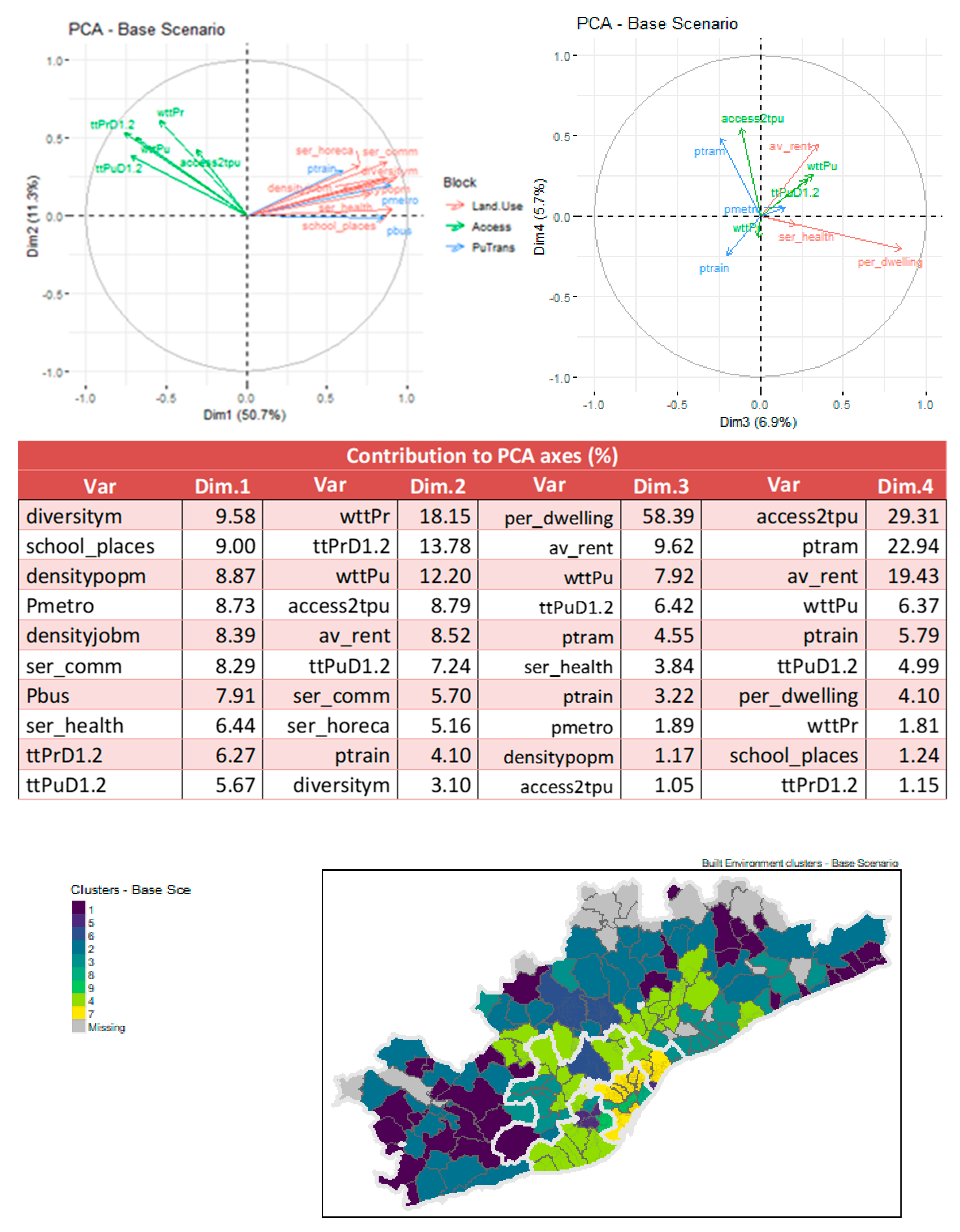
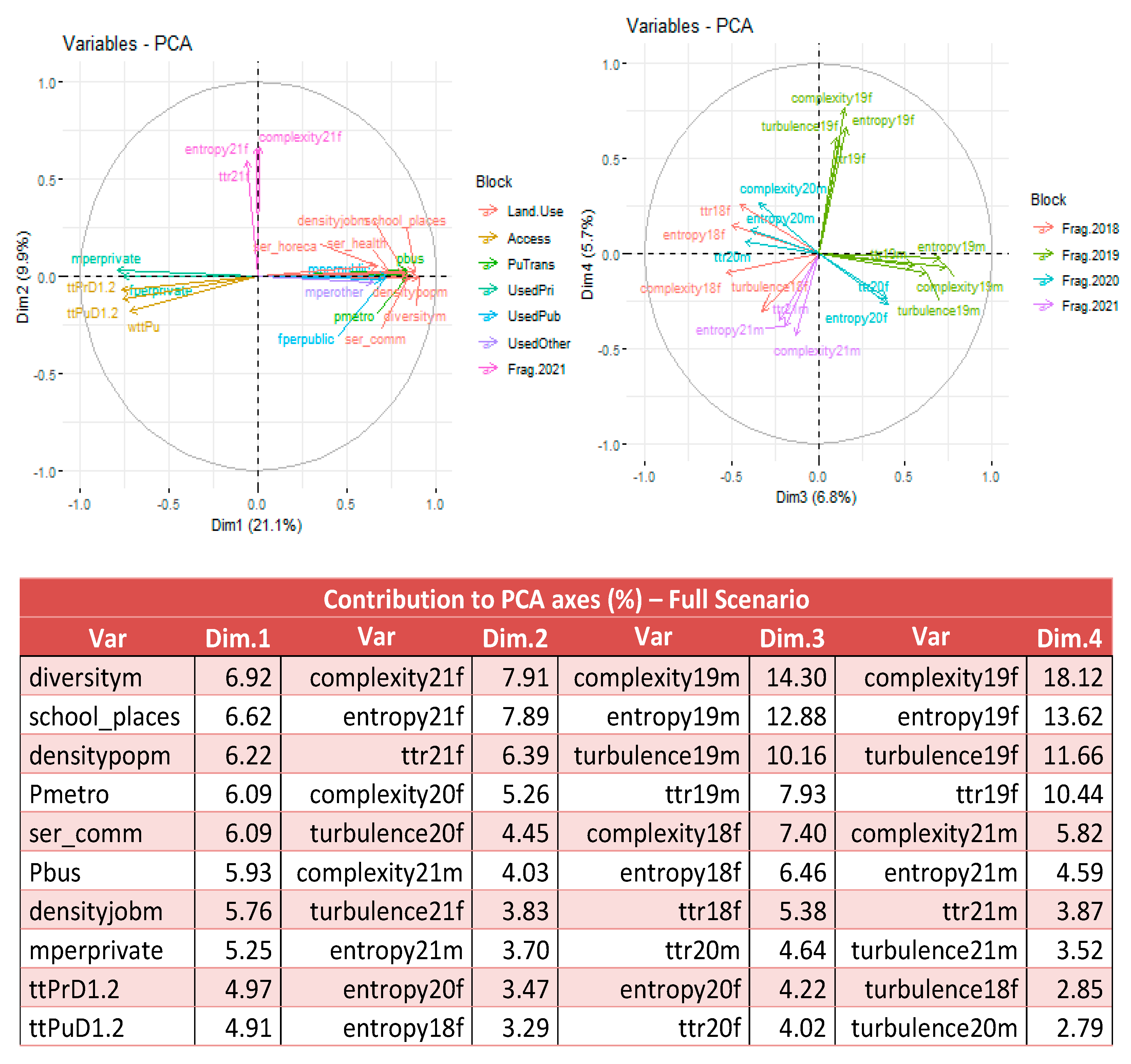
Figure 3. Full PCA analysis: contributions to the first to fourth dimensions in PCA and variable projections. Left, dimensions 1–2; right, dimensions 3–4.

7.2. Full Analysis Results

Principal Components (PCA) are linear combinations of the original variables considering, in this second analysis, variables V1 to V14 as active variables, transport mode preferences, fragmentation indicators, in blocks V15 to V20 by year and gender, and modal share and principal mode preference by gender. The variables contributing the most to the first four axes were:

Axis 1. The first axis is positively related to the amount of population and jobs and high land-use diversity; the number of bus, metro, and train public transport stops, with a high percentage of public transport use. This axis is negatively related to mean travel time to the CBD, either by private or public transport. This axis contraposes the density of activities inside and around the Barcelona city area to the travel time to the city centre. Municipalities, Barcelona city zones, and the primary crown are located (ETM) on the positive part of this axis.
Axis 2. This axis is related to increasing turbulence and complexity in 2018–2021 on the positive part of the axis.
Axis 3. The third axis is related to the increasing turbulence and complexity related to 2018–2020 on opposite parts of the axes, positive for men in 2019, and negative for women in 2018 and men in 2020.
Axis 4. The fourth axis is related to increasing fragmentation indicators related to 2019 and 2021 on opposite parts of the axes, positive for women in 2019, and negative for men in 2021 and women in 2020.

Figure 3 summarizes the contribution of the original variables to each factorial axis using graphs. They provide additional information, relevant for the case of the first principal component (first axis), because the socioeconomic and built environment variables provide opposite contributions.

Clusters were profiled according to the most significant numeric variables and factors of the zones included in the clusters [36]. The number of clusters was found to explain at least 50% of data variability. The most significant variables associated with the cluster definition were population density, mixed land use (diversity), job density, and number of public transport stops within the built environment block (in each TAZ), complexity and turbulence for women in 2020, and public and share of other transport modes.

Cluster 1. Travel time by private or public transport over the mean. Market share of public transport over the mean and men fragmentation indicators in 2020.
Cluster 2. Entropy and travel time in 2021 above the mean for both men and women. Very low incidence of nonmotorized travel modes. Here, only one cluster was found, including small villages in the outskirts of RMB, highlighted using the second darkest blue in Figure 4.
Cluster 3. Fully characterized by fragmentation indicators in different years.
Cluster 4. Travel time on public transport and share of private transport are very high. Turbulence and complexity in 2020 are below the mean.
Cluster 5. Very high private vehicle use share. Turbulence and complexity below the mean for women in 2020.
Cluster 6. Turbulence and complexity considerably above the mean in 2020, for both men and women. It only contains Vallgorguina, a municipality in the Montseny Natural Park area in the north of the metropolitan area (third crown). During the strict COVID-19 lockdown in Spain, many residents in Barcelona moved temporarily to their holiday residences in this area (dark green in Figure 4).
Cluster 7. Fragmentation indicators in 2019 and 2021 above the mean, and private transport share also above the mean.
Cluster 8. Per capita income below the mean and nonmotorized vehicle use above the mean. The cluster contains 63 municipalities, with relevant medium cities such as Sabadell, Terrassa, and Vilanova i la Geltrú (Figure 4 in light green).
Cluster 9. Population, job density and land-use diversity above the mean, including a high number of bus stops and large amount of services in general. Contains all districts in Barcelona city and the densely populated city of l’Hospitalet.

Figure 4. Full analysis: spatial clustering of TAZs. Airport is indicated.

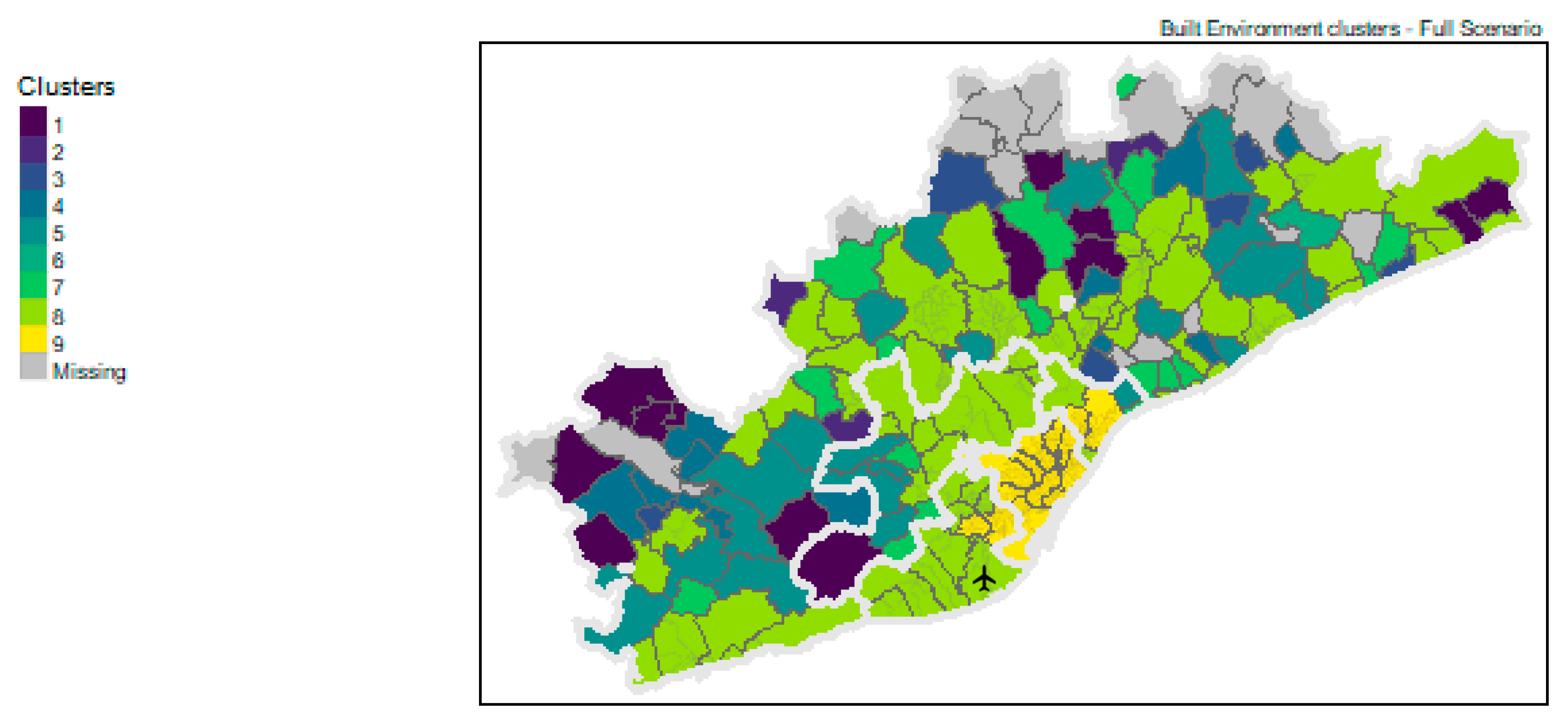
Spatial clusters in the full analysis were meaningful (Figure 4, light green and yellow): Barcelona city and the municipalities to the north (Badalona and Santa Coloma) and south (l’Hospitalet and Cornellà) form an urban continuum, densely populated and well-served by public transport. The south coast area is well-connected by train or bus to Barcelona city, and numerous commuters travel daily between these areas. The rest of the second crown in the interior contains Cerdanyola and Sant Cugat. These municipalities are extensively served by a local train to Barcelona, hosting many commuters every day. The rest of the third crown is diverse, but historical cities are included along the coast (Sabadell and Terrassa) and to the south (Sitges and Vilanova), which are well-served by train.

7.3. Full Analysis Results per Year

The justification for the third and fourth components was unclear, leading us to speculate that including all fragmentation variables for all years introduced noise that hindered the interpretation. If this was the case, a clearer picture would emerge if the analysis was repeated year by year, considering only the fragmentation variables for that specific year. Figure 5 shows the contributions of the variables to the PCA per year and their graphical representation on the PCA space, where stability can be noted across the years.

The analysis presents the percentages of variance explained by the first four principal components per year as follows:

2018: 36.8% (Dim 1); 10.7% (Dim2); 8.6% (Dim3); 7.0% (Dim4); 63.2% (Total);
2019: 36.8% (Dim 1); 11.3% (Dim2); 8.7% (Dim3); 7.1% (Dim4); 63.9% (Total);
2020: 36.9% (Dim 1); 10.6% (Dim2); 8.6% (Dim3); 7.1% (Dim4); 63.1% (Total);
2021: 36.8% (Dim 1); 12.1% (Dim2); 7:4% (Dim3); 7.2% (Dim4); 63.5% (Total).

The temporal stability of the first and second principal components is remarkable year after year. This is evidenced by in the explained variance, which remains nearly constant, and the variables that contribute to the explanation of the component. The first principal component is influenced by socioeconomic, built environment, and accessibility variables, whereas the second principal component is influenced by the fragmentation variables for each year. These results are highly consistent with those of the full analysis. The third and fourth principal components, which explain a marginal amount of the total variance, are explained by a mixture of variables. As a result, we decided to continue the analysis with the full set of variables only.

7.4. Full Analysis Revisited

A relevant issue in this study was the mode of transport most used by gender, where modes are classified between private (car, moto), public transport (bus, metro, train and tram) and others (i.e. bikes, walking or e-scooters). Figure 6 shows a remarkable difference between men and women: private modes are more used by men than women; again, the south of the primary crown shows a different gender pattern where the corridor represented by the historic cities of Sabadell and Terrassa.

A detailed analysis was conducted, highlighting the percentage of transport mode use in the spatial layout, with the results shown in Figure 6. More women than men used public transport in the primary crown. Private transport was used less in the primary crown than in the rest of the metropolitan area.

Figure 6. Percentage of transport mode use by zone and gender. EMEF data, 2018 to 2021.

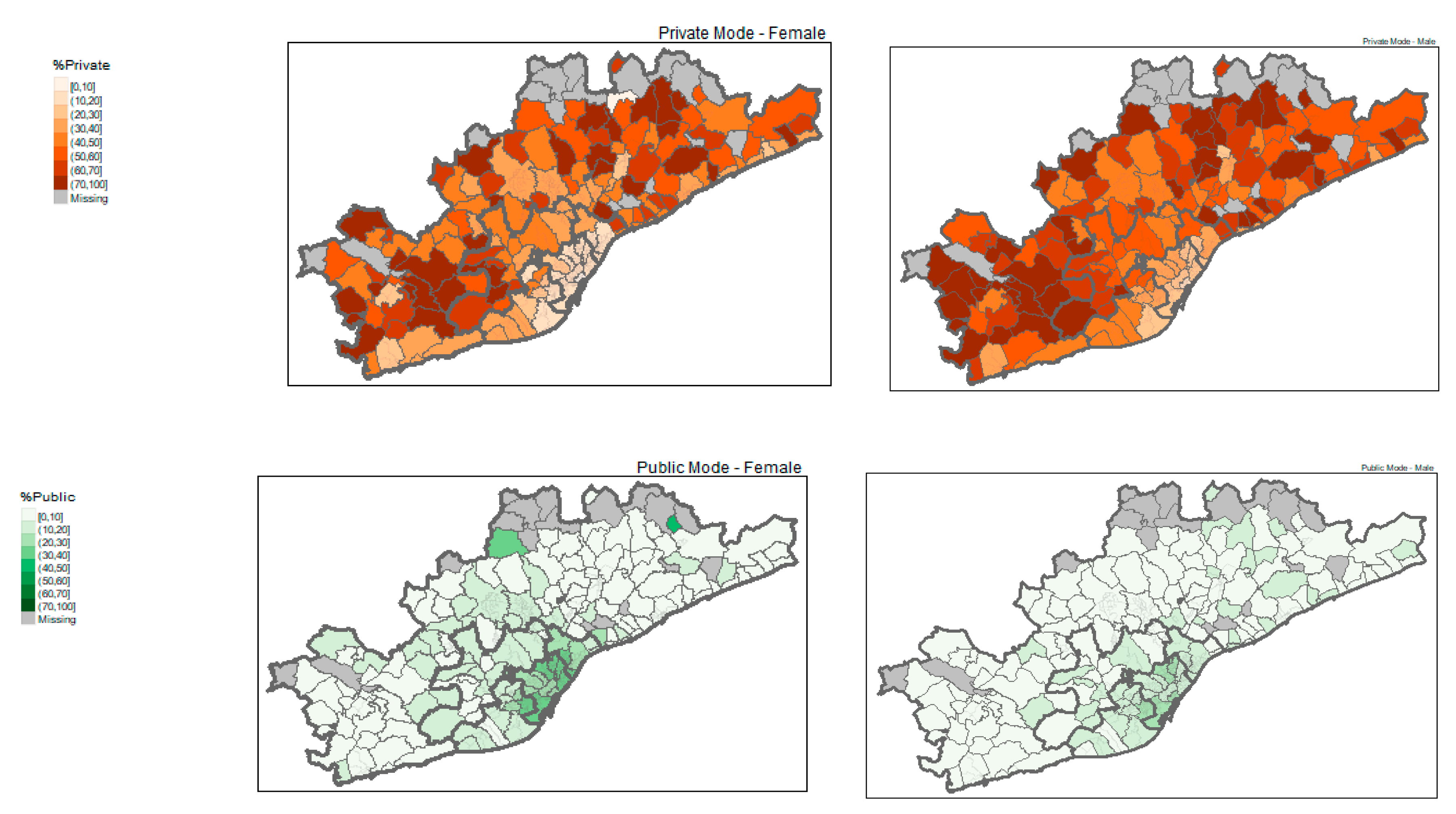
In the central part of Barcelona (primary crown/ETM), sustainable transport modes (public transport and others) were highly used by women, whereas in the zones in the rest of the AMB and RMB (the outer areas of the maps), the use of public transport was very low.

Accessibility to public transport at the origin and the share of transport mode by were not homogeneous. The coverage of public transport was nonuniform (upper Figure 7) in the metropolitan region; in the primary crown and some municipalities in the secondary crown, the density of public transport stops was high, showing the extra travel time required when using public transport to reach Barcelona’s CBD (lower Figure 7) by zone.

Figure 7. Number of public transport stops by zone (upper figure), extra travel time when using public transport to Barcelona’s CBD by zone (middle figure), and transport mode share by gender and number of public stops (lower figures with y-axis as discretized number of public transport stops by zone).

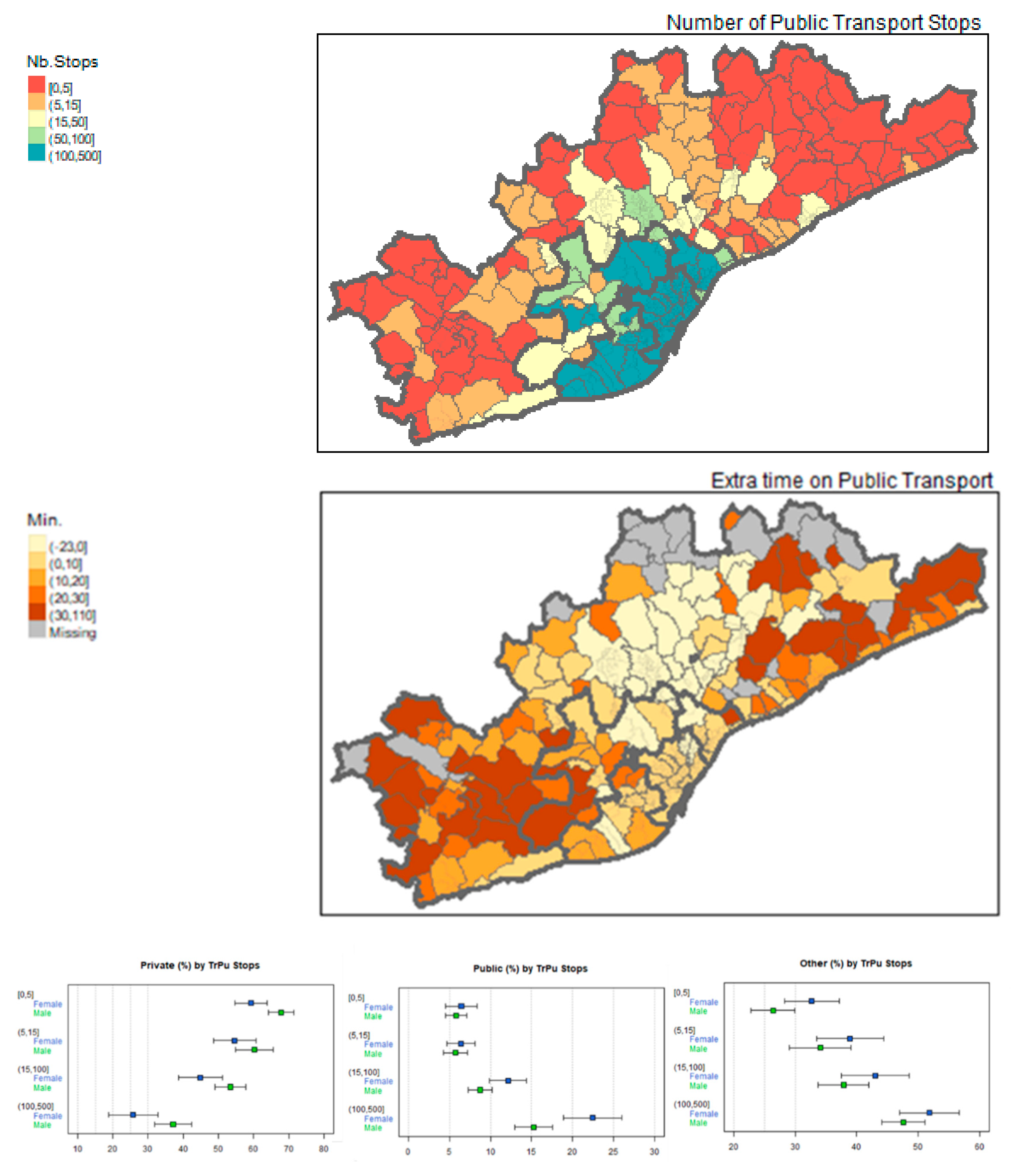
The extra time required when using public transport to access Barcelona’s CBD was remarkable for non-coastal areas, to the north and south, except for the Vallès corridor, to the historical cities which are well-served by train. For any range of extra travel time when using public transport compared with the use of private transport, the 95% confidence intervals of the mean entropy for men were greater than that for women. The confidence intervals did not intersect for the two groups with a less than 10 min average difference between public and private transport. Extra turbulence in the women’s group was found for municipalities such as Sant Just Desvern, Matadepera, Premià, Teià, Sant Pol, Calella, and Cabrera de Mar, which had a high per capita income: these municipalities do not have adequate public services (public transport stops are sparse).

Figure 7 (lower) shows how the density of public transport stops affected the use of public transport for the zones belonging to the crowns whose borders are highlighted in the maps (upper and middle in Figure 7). When the network was not dense, the percentage of use of private transport was higher by men than women. Women preferred to use nonmotorized transport (the percentage of use of other modes was higher than for men). Because women used public transport more than men, we analysed the effect on the turbulence fragmentation indicator. The turbulence variability was wider for women than for men, and the mean values are also higher due to the differences in activity patterns by gender (Figure 7, lower).

7.5. Optimal Spatial Clustering and Sequence Analysis (SA)

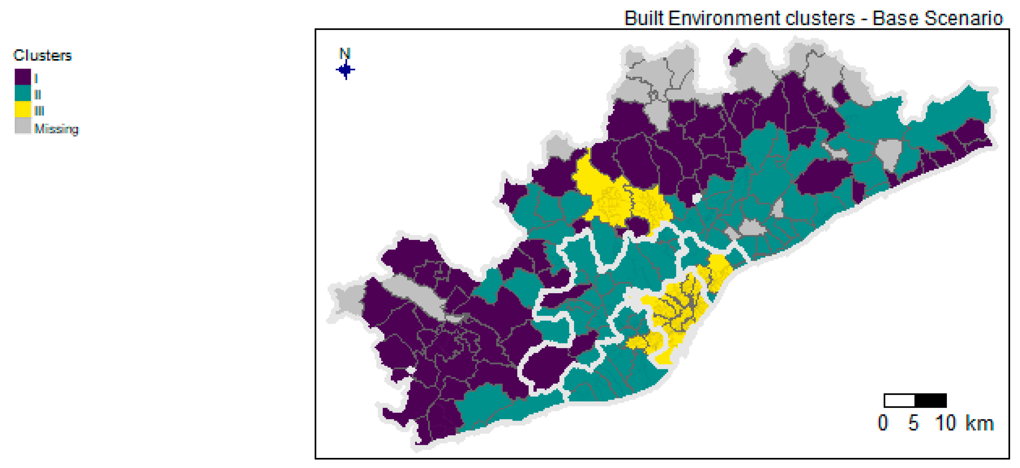
The built environment and land use spatial clusters explained 50% of the intercluster variability in the base analysis. The clustering analysis, which was evaluated by calculating the silhouette plot [41], proposes a partition based on three clusters. Figure 8 depicts the resulting clusters that highlight densely populated zones (in yellow, cluster III) in the first crown (EMT) and historical cities of Sabadell and Terrassa vs. medium-density zones (turquoise, cluster II) and mostly rural areas (dark blue, cluster I). For each spatial area, a hierarchical clustering of the sequences of travel behaviour in a day was performed leading to a set of subclusters for each spatial cluster I to III. The preliminary results for the densely populated subarea (including the first crown of the RMB) are shown in Figure 8.

We analysed the transport purposes and transport modes defining eleven activities, including home (H), work (W), casual (C, infrequently visited places), other (O, frequently visited places outside of work), school (S, students only), escorting (A), and the five travel categories: active (TW, walking and cycling), public transport (TP), traveling by car (TC), e-scooter (TE), and other travel categories (TM). The final analysis considered an alphabet list of 11 activities. Both trip makers and nontrip makers were included in a sequence of 1,440 minutes or more (for example, those returning home after midnight), with each minute classified according to a travel activity category.

We focused on spatial cluster III, which showed a state distribution for the five SA clusters, allowing an initial interpretation of the travel behaviour profiles represented by each cluster (Figure 9). State distribution is the proportion of the day invested in the different activities. The main results are:

Cluster III.1 represents mostly morning workers, some of them extending their shift throughout the days.
Cluster III.2 represents afternoon-shift workers.
Cluster III.3, a low incidence of work activity is highlighted, and the incidence of home-based activities is remarkable, but escorting and other recurrent (not work) activities occur during the day.
Cluster III.4 represents partial morning work and afternoon educational activities conducted by public transport.
Cluster III.5 accounts for morning educational activities that, in some cases, are extended to the afternoon, with almost no incidence of work activity or other recurrent late afternoon activities.

For a more detailed analysis of each spatial cluster, a subcluster refinement has been addressed considering the individual daily sequences inside each spatial-based cluster (clusters I to III). The silhouette plots determined the optimal number of subclusters for each spatial cluster was found to be two, three, and five, respectively. Figure 10 depicts the percentage of the SA subclusters in each TAZ-EMEF and spatial subcluster by gender. No graphical description of the state-distribution behavioural patterns in spatial clusters I and II is provided, but they can be easily described.

SA subclusters in spatial cluster I split activity sequences into educational-based (either morning or afternoon) using public transport (cluster I.1) and work-based using private transport (mostly morning shift), noting some immobility (whole day home-based) where people did not conduct other activities. In spatial group II, work-based sequence activities using either private or public transport are included in cluster II.1, whereas cluster II.2 contains home-based and other activities, with a remarkable use of active modes. Cluster II.3 groups daily education-based travel by public transport, for both morning and afternoon shifts.

Figure 9 shows the daily state distribution of the activities in the sequences belonging to spatial group III, split into men and women. Hierarchical clustering was repeated for each gender subsample and spatial cluster, and the four most remarkable clusters for each gender were analysed. In the clustering for the men, the characterization was easy to describe in the spatial cluster III (densely populated macrozones): morning work-dominated profiles that extend to the whole daily period in cluster III.5, afternoon work-dominated profiles in cluster III.4, educational profiles (in III.1), and home-based plus escorting profiles including part-time work in cluster III.2. The relative incidence of the spatial cluster III subclusters, for men, was 8%, 55%, 6%, and 31%, respectively (see Figure 9).

In subclusters for the women, the characterization was clear: work-based profiles that extended to the whole daily period in cluster III.5, afternoon educational and morning part-time work profiles in cluster III.3, morning educational profiles in cluster III.1, and home-based plus escorting profiles with limited part-time work in cluster III.2. The share of private car transport was lower for the women’s than the men’s clusters. The relative incidence of the spatial cluster III women’s subclusters was 6%, 60%, 3% and 31%, respectively, for subclusters 1,2, 3, and 5 (see Figure 9).

Figure 9. State distribution of activity sequences in spatial cluster III by gender (top, men; women, bottom). All years, based on EMEF survey data.

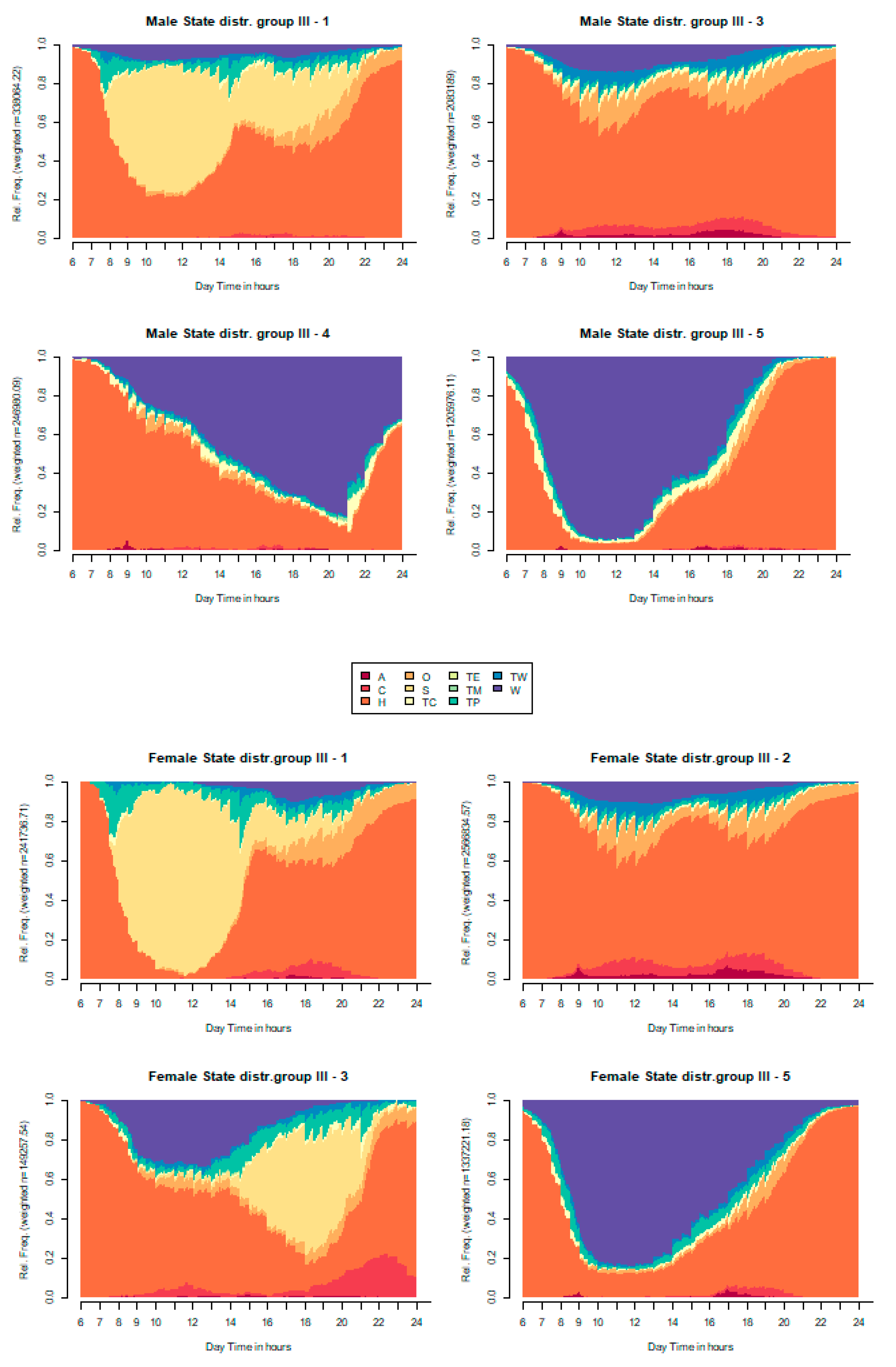
Transport for escorting purposes in spatial cluster III accounted for a mean of 11.25 min (standard deviation 48 min) for men and 14.52 min (standard deviation 50 min) for women, and travel for work had a mean of 234 min (standard deviation 266 min) for men and 186 min (standard deviation 239 min) for women. The 95th percentile of escorting time was 70 min for men and 95 min for women. The 95the percentile of travel time by car was 120 min (mean 29 min) for men and 85 min for women (mean 15 min). The 95th percentile of travel time by public transport was 120 min (mean 24 min) for men and 130 min for women (mean 35 min). These figures and the incidence of home-based profiles in group III for men and women confirm the previous findings.

Spatial clusters are based on land use and built environment variables (I to III) and a refinement in each spatial cluster based on activity sequences has been conducted and provides subclusters whose incidence are described in Figure 10.

Figure 10. Percentage of SA subclusters for spatial clusters I to III.

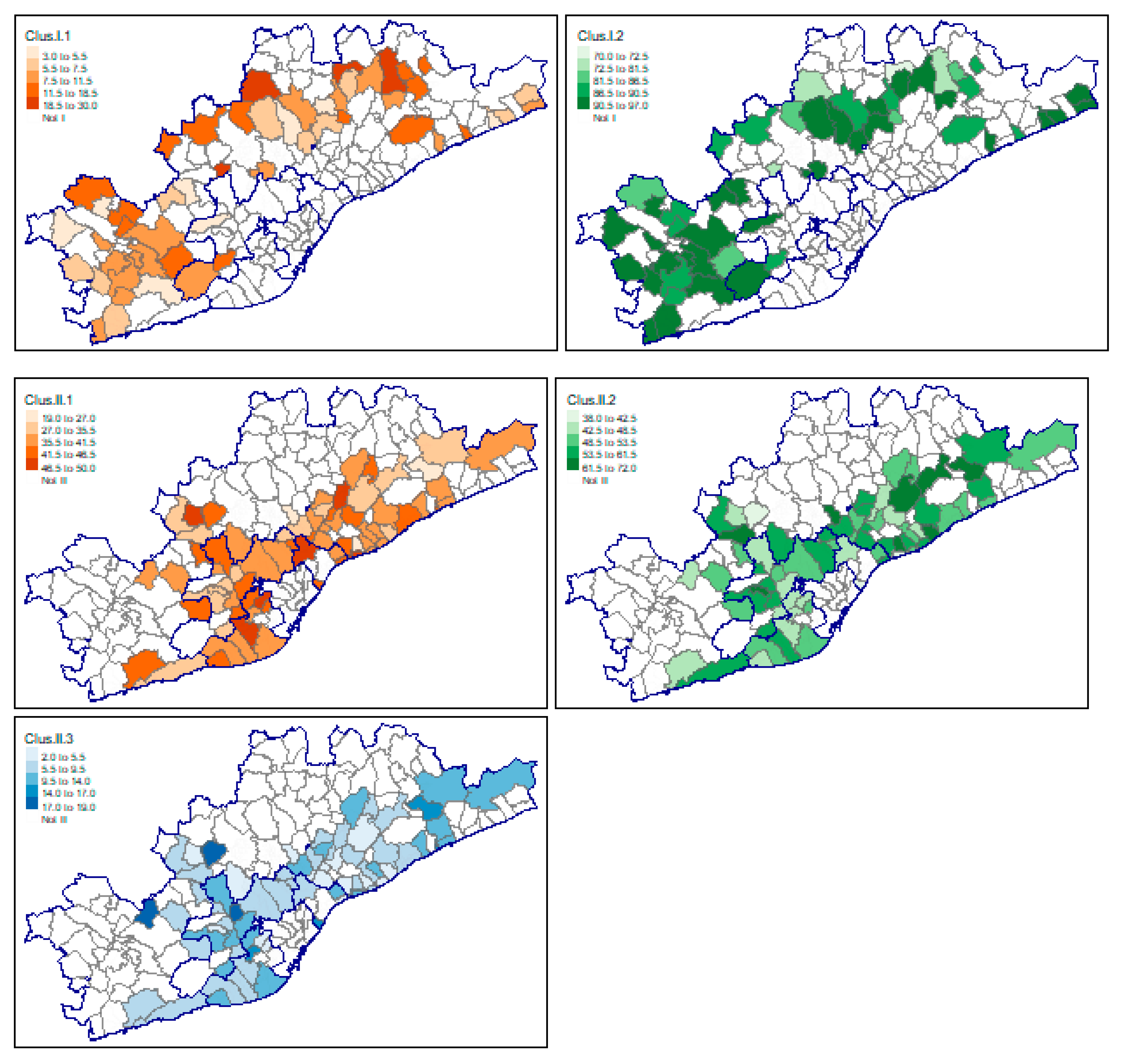
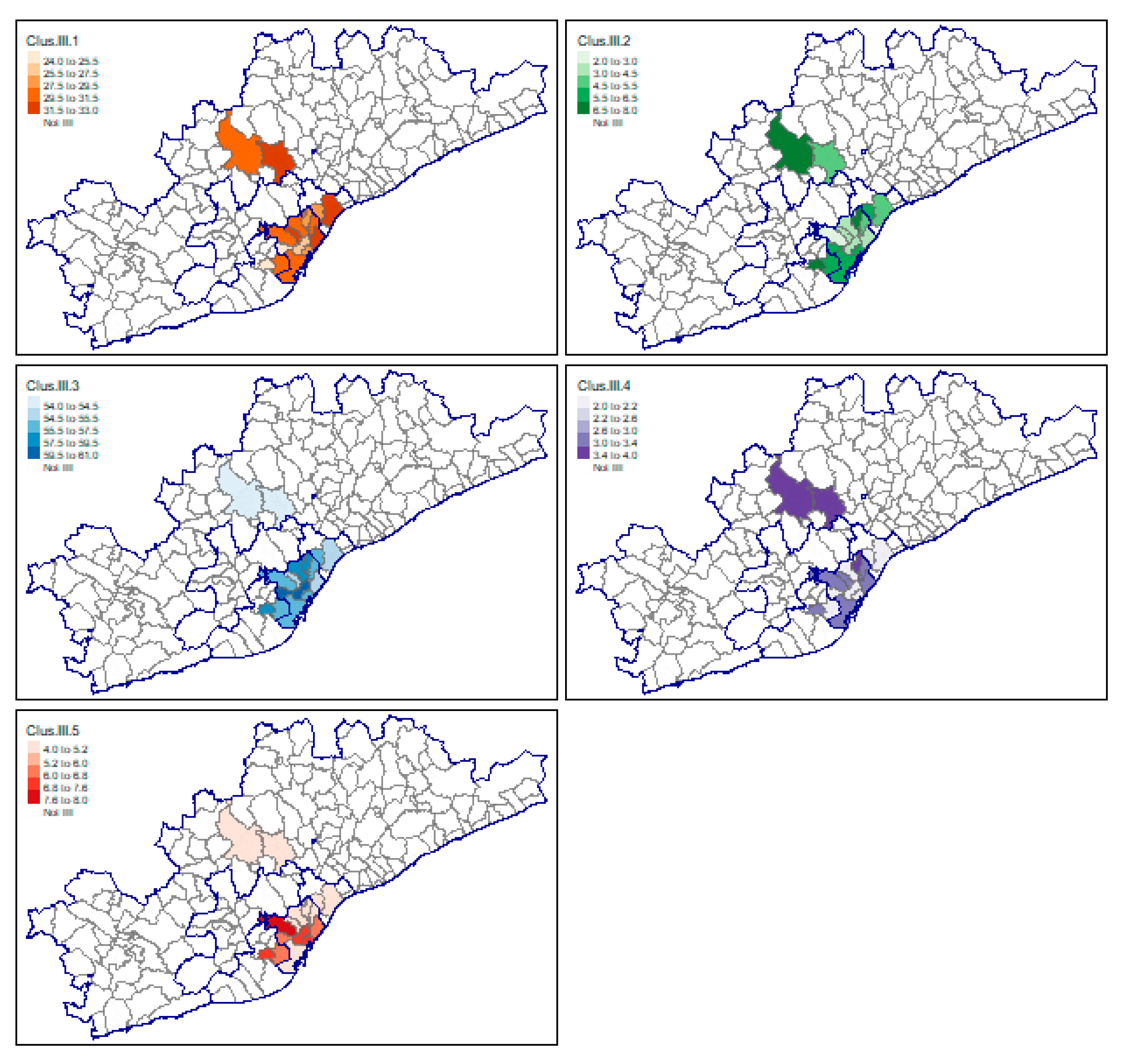
Cluster III.5, constituted by dedicated students, was over-represented in the Sarrià, Sant Martí, and Eixample districts in Barcelona city, whereas morning-shift workers was over-represented in Sabadell and Badalona (both densely populated cities in the RMB). Home-based activity was remarkable in the Eixample and les Corts districts in Barcelona. Transport for part-time work and education was higher in the Sabadell and Terrassa historical cities in the RMB.

8. Discussion and Conclusions

In this study, we focused on how the built environment influences mobility patterns considering individual characteristics and the spatial arrangement of the city of Barcelona. For that, we have used a thorough dataset and different variables, including land use, transportation, and socioeconomical variables, together with sequence analysis and fragmentation indicators.

In this respect, our initial hypothesis was that fragmentation indicators played a critical role in the spatial clustering of the TAZs. This hypothesis was confirmed. Furthermore, they were found to be year-independent, which confirmed the accurate joint use of all EMEF surveys between 2018–2021. Regarding the results, they prove how the socioeconomic and spatial inequalities in the RMB, along with other factors, influence travel behaviour. Sustainable transport modes are mainly used in the inner part of Barcelona, which has been achieved through different policies with regard to sustainable mobility and urban planning (zones 30, low emissions zones, and the superblocks). However, our analysis suggested that sustainable transport options are barely used in the outer zones of Barcelona. According to the fragmentation indicators, we observed that those in suburban areas tend to use a private car to commute and that the complexity of the trips increases from these areas. Gender plays an important role in shaping mobility and sustainable mobility practices.

In this study, we observed important differences regarding gender, the built environment, and the spatial characteristics of the residential area. Our contribution shows that these characteristics should be considered to improve these modelling approaches.

Activity sequence clusters were different between men and women depending on the resident TAZ and the spatial cluster it belongs to. In previous studies, activity sequence clusters, not considering spatial grouping, were found to be significantly different [44].

We are aware of the limitations of the public data used in this study because we were able to analyse mobility for two gender groups. Diversity information was not included when collecting the surveys. Including this information would enrich the results, which could be used to provide insightful policy recommendations.

This study opens the door to further research. The changes produced by the COVID-19 pandemic need to be further investigated, as people may return to previous mobility patterns, despite many people transitioning to online activities, such as e-commerce or working from home, due to the pandemic restrictions. New data from EMEF travel surveys (from 2022) include family structure and teleworking questions, which will be considered in future analyses of behavioural patterns.

The current approaches for analysing transportation are based on agent-based travel demand models, which require the definition of synthetic populations that are usually characterized based on activity profiles [45,46,47,48,49], however, we consider that further refinements are necessary to more realistically represent the behavioural aspects of the population in the direction initially explored by [13], and find how they could be appropriately included in these transport models to support tailored transport policies, as declared in the objectives of this paper as a future research topic.

Author Contributions

Conceptualization, L.M., L.M.D. and J.B.; formal analysis, L.M., L.M.D. and J.B.; funding acquisition, L.M. and J.B.; methodology, L.M., L.M.D. and J.B.; software, L.M.; supervision, J.B.; writing—original draft, L.M.; writing—review and editing, L.M.D. and J.B. All authors have read and agreed to the published version of the manuscript.

Funding

This research was funded by Spanish R+D Programs (PID2020-112967GB-C31) and by Secretaria d’Universitats-i-Recerca-Generalitat de Catalunya—2021 SGR 01252 Information Modeling and Processing.

Data Availability Statement

Restrictions apply to the availability of EMEF data. Anonymized data were obtained from the Autoritat del Transport Metropolità (ATM) and datasets cannot be distributed without their permission.

Acknowledgments

EMEF datasets, previously processed, were kindly shared by the Autoritat del Transport Metropolità (ATM). Their contribution to our research is gratefully acknowledged

Conflicts of Interest

The authors declare no conflict of interest.

Appendix A

Table A1. Land use, transportation, and socioeconomical variables.

Variable	Type	Source	Original Zoning System	Year	TAZ data
Total roof area	Area	Land registry https://www.sedecatastro.gob.es/	Ground plots	2019	Roof area in m² according to 16 types
Inhabitants by age group	Population	Population census IDESCAT	Census tracts	2019	Number of inhabitants by age group (4 groups)
Inhabitants by education level	Population	Population census IDESCAT	Census tracts	2011	Number of inhabitants by education (4 groups)
Mean Income per Capita (Mean)	Population	IDESCAT (Catalan Institute of Statistics)	Census tracts	2016	Mean per capita income
Dwelling and dwelling size	Dwelling units	Population census AMB	Census tracts	2011	Number of dwelling units and dwelling size in 4 groups
Dwelling surface	Dwelling units	Population census AMB	Census tracts	2011	Number of dwelling units by dwelling surface group (4 groups)
Parking areas	Parking	AMB	Ground plots	2019	m² of ceiling
Residential type	Type of residential area	AMB	Ground plots	2017	m² used by old city, blocks, urban blocks and isolated dwelling units
Services	Services	AMB	POIs	2019	Number of services according to 16 types
Educational buildings	Services	AMB	POIs	2019	Number of students
Urban bus-stops	Transport data	GTFS	Dots	2019	Urban bus stops
Metropolitan bus-stops	Transport data	GTFS	Dots	2019	Metropolitan bus-stops
International bus-stops	Transport data	AMB	Dots	2019	International bus-stops
Metro-stops	Transport data	GTFS	Dots	2019	Metro stops
Tram-stops	Transport data	GTFS	Dots	2019	Tram stops
Taxi-stops	Transport data	AMB	Dots	2019	Taxi stations
Train stations	Transport data	GTFS	Dots	2019	Number of train stations in each TAZ
Metropolitan train stations	Transport data	GTFS	Dots	2019	Number of metropolitan train stations in each TAZ

Table A2. Fragmentation indicators used in this study.

Index (references)	Description	Formula	No.
Entropy [23,50]	Provides a measure of variety in daily schedules and represents the proportion of total time spent in each state. $π_{i}$ is the proportion of occurrences of the ith state in the specific sequence, S is the number of potential states, $x$ is the sequence of daily activities defined from minute to minute, and function log() refers to natural logarithm. Calculated based on the proportion of minutes allocated to each state during a day. This measure disregards the number of state changes and the specific ordering of states in the sequence. Visiting several states increases their entropy value whereas no state changes during the entire day is equal to a zero-entropy value. The potential value ranges depends on the number of states, with the maximum value achieved when the sequence evenly distributes time among all states. Therefore, a normalized entropy score is commonly used, dividing the entropy by the maximum entropy value, thus obtaining a range of 0 to 1.	$h (x) = h (π_{1} \dots π_{S}) = - \sum_{i = 1}^{S} π_{i} l o g (π_{i})$	(2)
Turbulence Elzinga and Liefbroer [22,24]	Measures the number of state recurrences and the variability in durations of daily activities. Based on sequence permanence and employs two components: number of distinct subsequences that can be derived from the distinct state sequence; the variance of consecutive time points spent in a distinct state. For a given sequence $x$ , the turbulence $T (x)$ considers: $ϕ (x)$ is the number of distinct subsequences that can be extracted from the distinct state sequence, considering time precedence; $s^{2}$ is the variance for the state duration; $s_{m a x}^{2}$ is the maximum variance, based on the sequence duration, computed as $s_{m a x}^{2} = (n - 1) {(1 - \bar{t})}^{2}$ , where n-1 is the number of transitions in the sequence and $\bar{t}$ is the sequence duration divided by the number of distinct states in the sequence.	$T (x) = {l o g}_{2} (ϕ (x) \frac{s_{m a x}^{2} + 1}{s^{2} + 1})$	(3)
Complexity [22,23]	A normalized score [0,1] based on the entropy and considers both the order of successive states, measured by transitions, and the distribution of different states. $n t (x)$ is the number of distinct transitions within a sequence, $l (x)$ is the length of the sequence, $h (x)$ is the entropy indicator, and $h_{m a x}$ is the maximum entropy in the sample. This index has a [0 ,1] value, with 0 corresponding to no transitions (e.g., staying at home the entire day). A more sensitive indicator than entropy.	$C (x) = \sqrt{(\frac{n t (x)}{(l (x) - 1)} \frac{h (x)}{h_{m a x}})}$	(4)
Travel time ratio (TTR) [24,51]	Trade-offs that people make between travel time and activity time. Herein, TTR is calculated as total time spent on daily activities ( $T_{t}$ ), divided by the sum of the total time at home ( $T_{s})$ plus the total time on daily activities ( $T_{t}$ ). TTR ranges from 0.5 (no trips made) to 1.0 (entire day spent away from home).	$τ = \frac{T_{t}}{T_{t} + T_{s}}$	(5)

References

Lefebvre, H.; Hess, R.; Deulceux, Sandrine.; Weigand, Gabriele.; Normandie roto impr.) Le Droit À La Ville; Economica-Anthropos, 2009; ISBN 9782717857085.
2016; 2. UN The New Urban Agenda | Urban Agenda Platform; 2016;
Kadi, J.; Matznetter, W. The Long History of Gentrification in Vienna, 1890–2020. City 2022, 26, 450–472. [CrossRef]
Cooper, A.; Kurzer, P. Similar Origins – Divergent Paths: The Politics of German and Dutch Housing Markets. Ger Polit 2023, 32, 341–360. [CrossRef]
Loomans, D. Long-Term Housing Challenges: The Tenure Trajectories of EU Migrant Workers in the Netherlands. Hous Stud 2023. [CrossRef]
Joint-Research-Center, (European-Comission); Mejía-Dorantes, L.; Murauskaite-Bull, I. Transport Poverty – A Systematic Literature Review in Europe; PUBLICATIONS, E., Ed.; Publications Office of the EU, 2022; ISBN https://data.europa.eu/doi/10.2760/793538. [CrossRef]
Ferrer-Ortiz, C.; Marquet, O.; Mojica, L.; Vich, G. Barcelona under the 15-Minute City Lens: Mapping the Accessibility and Proximity Potential Based on Pedestrian Travel Times. Smart Cities 2022, 5, 146–161. [CrossRef]
Gil-Alonso, F.; López-Villanueva, C.; Thiers-Quintana, J. Transition towards a Sustainable Mobility in a Suburbanising Urban Area: The Case of Barcelona. Sustainability 2022, 14. [CrossRef]
Cubells, J.; Marquet, O.; Miralles-Guasch, C. Gender and Age Differences in Metropolitan Car Use. Recent Gender Gap Trends in Private Transport. Sustainability (Switzerland) 2020, 12. [CrossRef]
Montero, L.; Mejía-Dorantes, L.; Barceló, J. The Role of Life Course and Gender in Mobility Patterns: A Spatiotemporalsequence Analysis in Barcelona. European Transport Research Review 2023, 15. [CrossRef]
Rasouli, S.; Timmermans, H. Activity-Based Models of Travel Demand: Promises, Progress and Prospects. International Journal of Urban Sciences 2014, 18, 31–60. [CrossRef]
Sidharthan, R.; Bhat, C.; Pendyala, R.; Goulias, K. Model for Children’s School Travel Mode Choice. 2011, 78–86. [CrossRef]
Shi, H.; Su, R.; Xiao, J.; Goulias, K.G. Spatiotemporal Analysis of Activity-Travel Fragmentation Based on Spatial Clustering and Sequence Analysis. J Transp Geogr 2022, 102, 103382. [CrossRef]
Abbott, A. Sequences of Social Events: Concepts and Methods for the Analysis of Order in Social Processes. Historical Methods: A Journal of Quantitative and Interdisciplinary History 1983, 16, 129–147. [CrossRef]
Abbott, A. Event Sequence and Event Duration: Colligation and Measurement. Historical Methods: A Journal of Quantitative and Interdisciplinary History 1984, 17, 192–204. [CrossRef]
Abbott, A.; Forrest, J. Optimal Matching Methods for Historical Sequences. Journal of Interdisciplinary History 1986, 16, 471. [CrossRef]
Abbott, A.; Tsay, A. Sequence Analysis and Optimal Matching Methods in Sociology: Review and Prospect. Sociol Methods Res 2000, 29, 3–33. [CrossRef]
Leszczyc, P.T.L.P.; Timmermans, H. Unconditional and Conditional Competing Risk Models of Activity Duration and Activity Sequencing Decisions: An Empirical Comparison. J Geogr Syst 2002, 4, 157–170. [CrossRef]
McBride, E.C.; Davis, A.W.; Goulias, K.G. Sequence Analysis of Place-Travel Fragmentation in California. Mapping the Travel Behavior Genome 2020, 371–398. [CrossRef]
Studer, M.; Ritschard, G. What Matters in Differences between Life Trajectories: A Comparative Review of Sequence Dissimilarity Measures on JSTOR. Journal of the Royal Statistical Society A 2016, 179, 481–511.
Ritschard, G. Measuring the Nature of Individual Sequences. Sociol Methods Res 2021, 1–34. [CrossRef]
Elzinga, C.H.; Liefbroer, A.C. De-Standardization of Family-Life Trajectories of Young Adults: A Cross-National Comparison Using Sequence Analysis. European Journal of Population 2007, 23, 225–250. [CrossRef]
Gabadinho, A.; Ritschard, G.; Studer, M.; Müller, N.S. Mining Sequence Data in R with the TraMineR Package: A User s Guide; Department of Econometrics and Laboratory of Geograpghy (University of Geneve): Geneve (Switzerland), 2011;
McBride, E.; Davis, A.; Goulias, K. Fragmentation in Daily Schedule of Activities Using Activity Sequences: Transportation Researc Record 2019, 2673, 844–854. [CrossRef]
Liao, T.F.; Bolano, D.; Brzinsky-Fay, C.; Cornwell, B.; Fasang, A.E.; Helske, S.; Piccarreta, R.; Raab, M.; Ritschard, G.; Struffolino, E.; et al. Sequence Analysis: Its Past, Present, and Future. Soc Sci Res 2022, 107, 102772. [CrossRef]
Su, R.; McBride, E.C.; Goulias, K.G. Pattern Recognition of Daily Activity Patterns Using Human Mobility Motifs and Sequence Analysis. Transp Res Part C Emerg Technol 2020, 120, 102796. [CrossRef]
Goulias, K.G.; McBride, E.C.; Su, R. Life Cycle Stages, Daily Contacts, and Activity-Travel Time Allocation for the Benefit of Self and Others. Mobility and Travel Behaviour Across the Life Course 2020, 206–220. [CrossRef]
Rokach, L.; Maimon, O. Clustering Methods. Data Mining and Knowledge Discovery Handbook 2005, 321–352. [CrossRef]
Grubesic, T.H.; Wei, R.; Murray, A.T. Spatial Clustering Overview and Comparison: Accuracy, Sensitivity, and Computational Expense. Annals of the Association of American Geographers 2014, 104, 1134–1156. [CrossRef]
von Behren, S.; Hilgert, T.; Kirchner, S.; Chlond, B.; Vortisch, P. Image-Based Activity Pattern Segmentation Using Longitudinal Data of the German Mobility Panel. Transp Res Interdiscip Perspect 2020, 8, 100264. [CrossRef]
Mobility Observatory in Catalonia (OMC) - ATM Working Day Mobility Surveys (EMEF) Available online: https://omc.cat/en/w/surveys-emef (accessed on 22 June 2024).
ENQUESTES DE MOBILITAT - Institut Metropoli Available online: https://www.institutmetropoli.cat/ca/enquestes/enquestes-de-mobilitat/#1447843451840-2-0 (accessed on 8 September 2023).
Montero, L.; Mejía-Dorantes, L.; Barceló, J. Applying Data Analytics to Analyze Activity Sequences for an Assessment of Fragmentation in Daily Travel Patterns: A Case Study of the Metropolitan Region of Barcelona. Sustainability 2023, Vol. 15, Page 14213 2023, 15, 14213. [CrossRef]
PTV AG VISUM 2020.
Husson, F.; Lê, S. EXPLORATORY MULTIVARIATE ANALYSIS BY EXAMPLE USING R.; CRC PRESS, 2020; ISBN 9780367658021.
Husson, F.; Josse, J.; Lê, S.; Mazet, J. FactoMineR: Exploratory Multivariate Data Analysis with R 2008.
RStudio-Team RStudio: Integrated Development for R. 2022.
Nielsen, F. Introduction to HPC with MPI for Data Science. 2016. [CrossRef]
Kaufman, L.; Rousseeuw, P.J. Finding Groups in Data; Wiley Series in Probability and Statistics; Wiley, 1990; ISBN 9780471878766.
Ward, J.H. Hierarchical Grouping to Optimize an Objective Function. J Am Stat Assoc 1963, 58, 236. [CrossRef]
Rousseeuw, P.J. Silhouettes: A Graphical Aid to the Interpretation and Validation of Cluster Analysis. J Comput Appl Math 1987, 20, 53–65. [CrossRef]
Gabadinho, A.; Ritschard, G.; Müller, N.S.; Studer, M. Analyzing and Visualizing State Sequences in R with TraMineR. J Stat Softw 2011, 40, 1–37. [CrossRef]
Lê, S.; Josse, J.; Husson, F. FactoMineR: An R Package for Multivariate Analysis. J Stat Softw 2008, 25, 1–18. [CrossRef]
Montero, L.; Mejía-Dorantes, L.; Barceló, J. Applying Data Analytics to Analyze Activity Sequences for an Assessment of Fragmentation in Daily Travel Patterns: A Case Study of the Metropolitan Region of Barcelona. Sustainability 2023, Vol. 15, Page 14213 2023, 15, 14213. [CrossRef]
Axhausen, K.W.; Gärling, T. Activity-based Approaches to Travel Analysis: Conceptual Frameworks, Models, and Research Problems. Transp Rev 1992, 12, 323–341. [CrossRef]
Bhat, C.R.; Goulias, K.G.; Pendyala, R.M.; Paleti, R.; Sidharthan, R.; Schmitt, L.; Hu, H.H. A Household-Level Activity Pattern Generation Model with an Application for Southern California. Transportation (Amst) 2013, 40, 1063–1086. [CrossRef]
Kitamura, R.; Chen, C.; Pendyala, R.M. Generation of Synthetic Daily Activity-Travel Patterns. Transp Res Rec 1997, 154–162. [CrossRef]
Horni, A.; Charypar, D.; Axhausen, K.W. Variability in Transport Microsimulations Investigated With the Multi-Agent Transport Simulation MATSim. Arbeitsberichte Verkehrs- und Raumplanung 2011, 692. [CrossRef]
Miller, E.J.; Roorda, M.J. Prototype Model of Household Activity-Travel Scheduling. Transp Res Rec 2003, 114–121. [CrossRef]
McBride, E.; Davis, A.; Goulias, K. Exploration of Statewide Fragmentation of Activity and Travel and a Taxonomy of Daily Time Use Patterns Using Sequence Analysis in California. Transp Res Rec 2020, 2674, 38–51. [CrossRef]
Dijst, M.; Vidakovic, V. Travel Time Ratio: The Key Factor of Spatial Reach. Transportation (Amst) 2000, 27, 179–199. [CrossRef]

Figure 1. Metropolitan Region of Barcelona: “Crowns” and TAZ-EMEF.

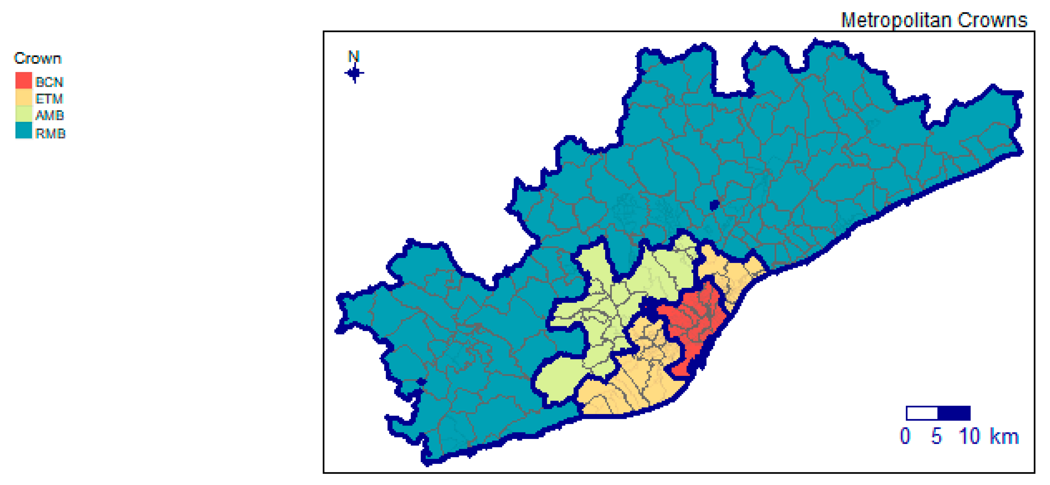
Figure 5. PCA results per year. Data sources: 2018–2021 EMEF surveys and land use and built environment data.

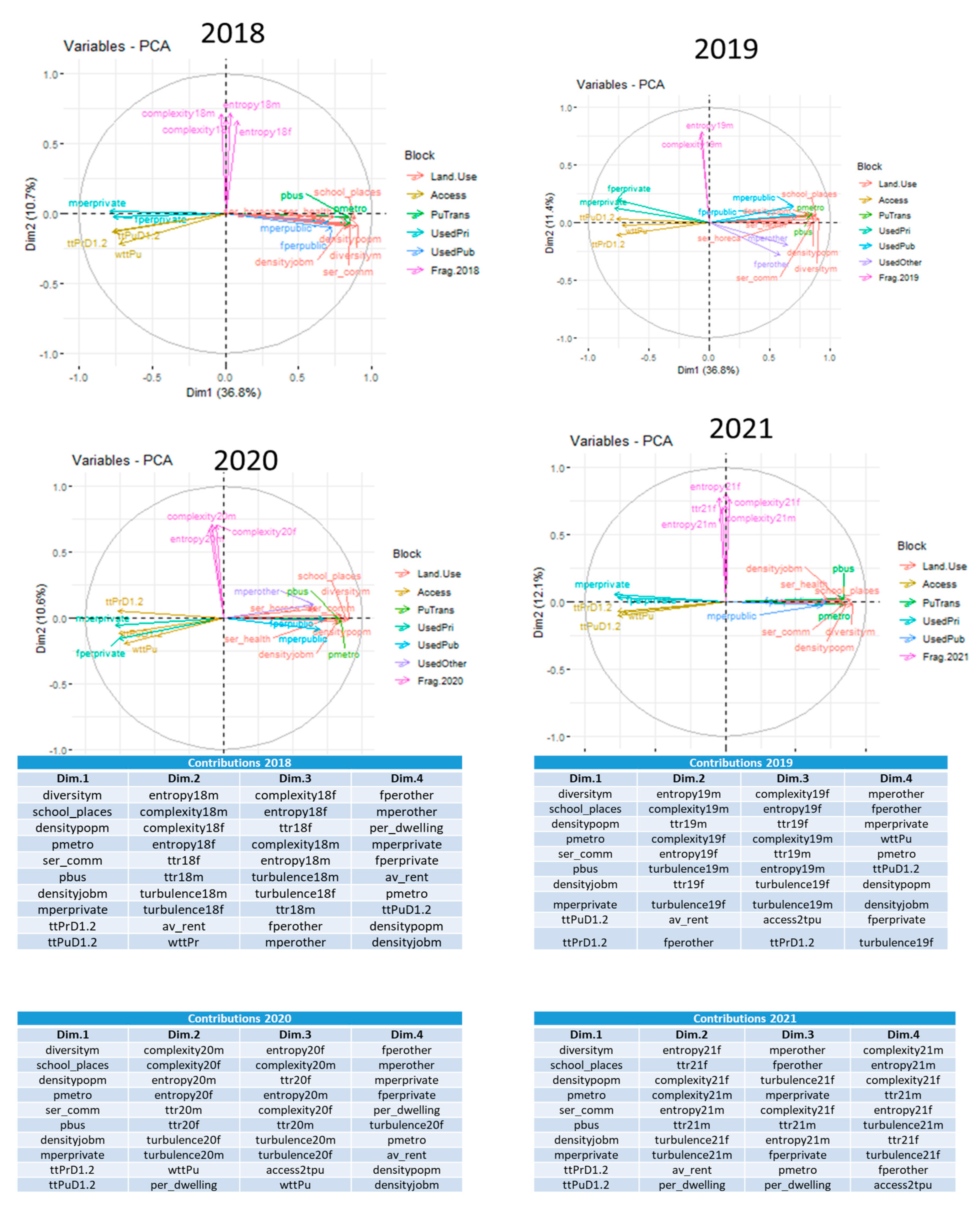
Figure 8. Optimal spatial clustering according to base analysis variables.

Disclaimer/Publisher’s Note: The statements, opinions and data contained in all publications are solely those of the individual author(s) and contributor(s) and not of MDPI and/or the editor(s). MDPI and/or the editor(s) disclaim responsibility for any injury to people or property resulting from any ideas, methods, instructions or products referred to in the content.

© 2024 by the authors. Licensee MDPI, Basel, Switzerland. This article is an open access article distributed under the terms and conditions of the Creative Commons Attribution (CC BY) license (http://creativecommons.org/licenses/by/4.0/).

Copyright: This open access article is published under a Creative Commons CC BY 4.0 license, which permit the free download, distribution, and reuse, provided that the author and preprint are cited in any reuse.