Preprint
Article

This version is not peer-reviewed.

How Frequent Is an Extraordinary Episode of Precipitation? Spatially-Integrated Frequency in the Júcar-Turia System (Spain)

Submitted:

06 January 2026

Posted:

07 January 2026

You are already at the latest version

Abstract

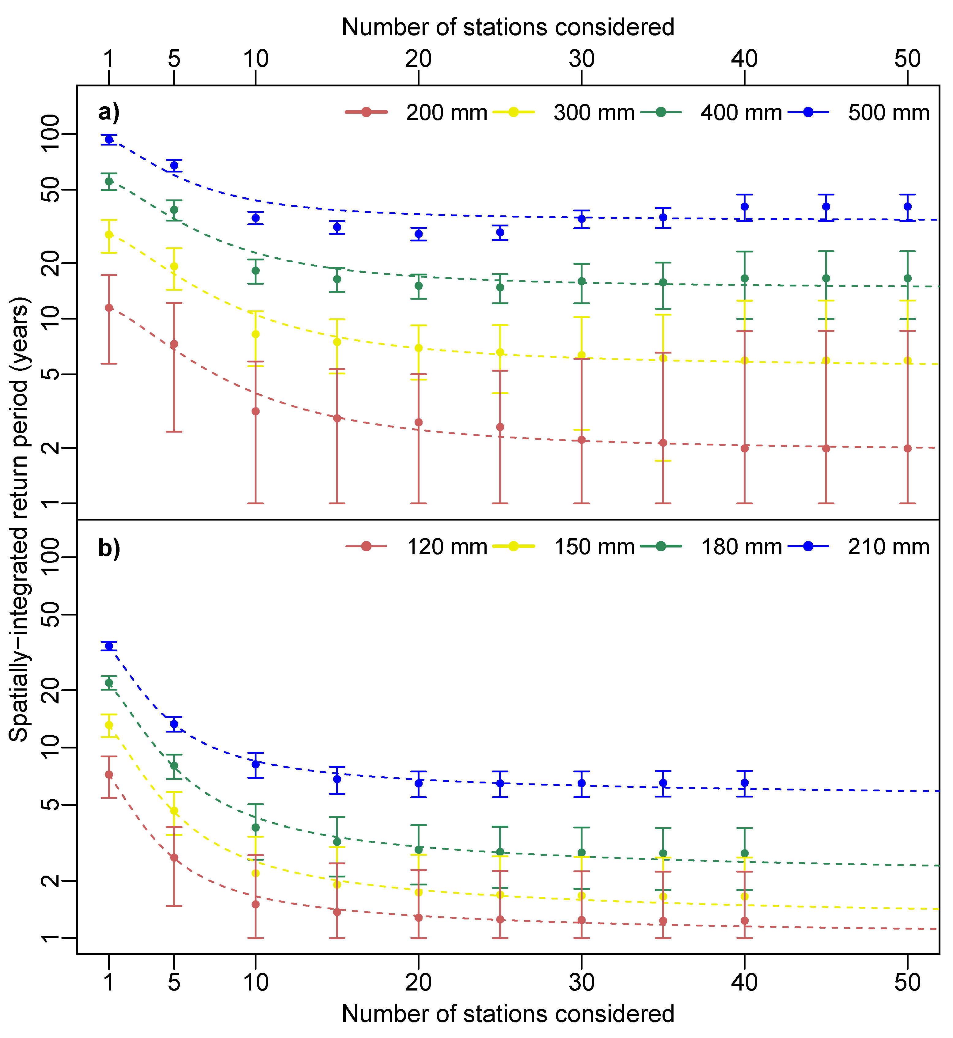
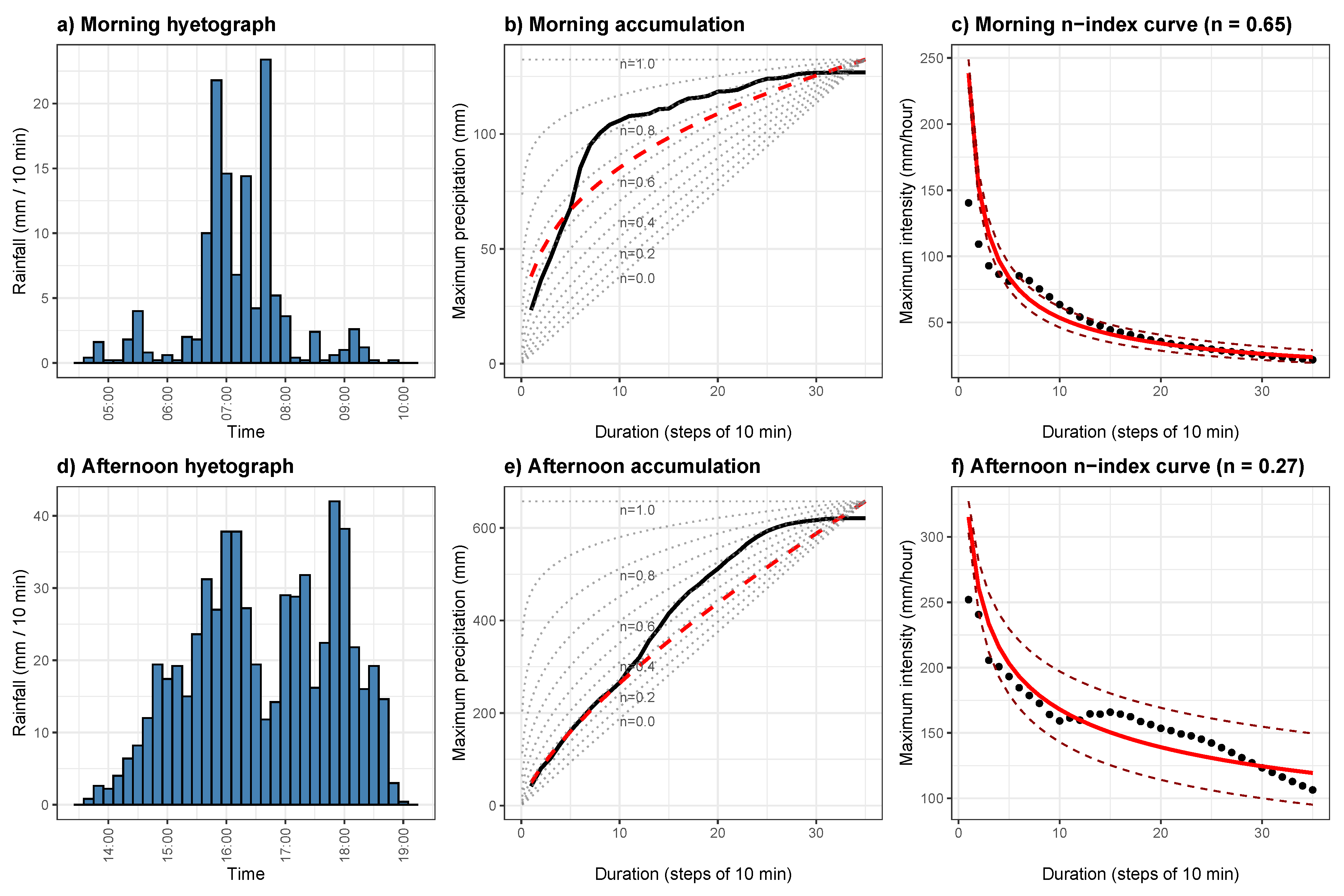
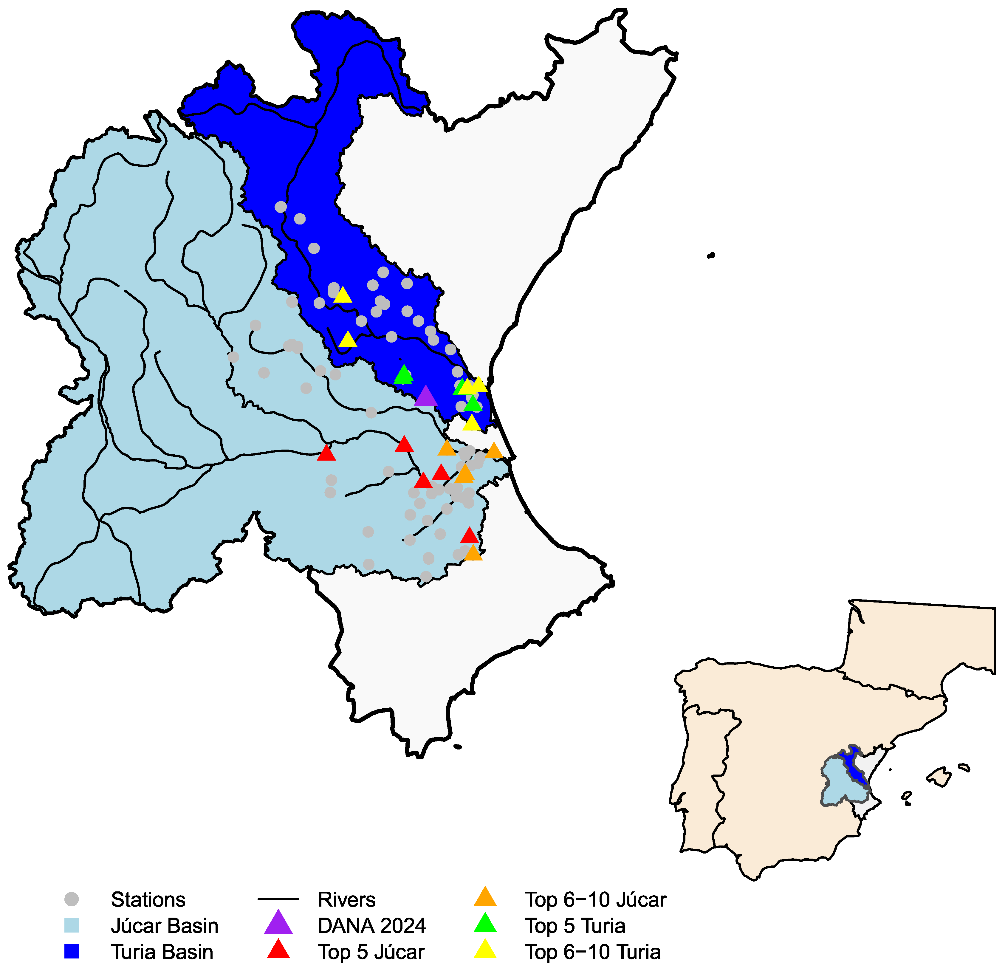
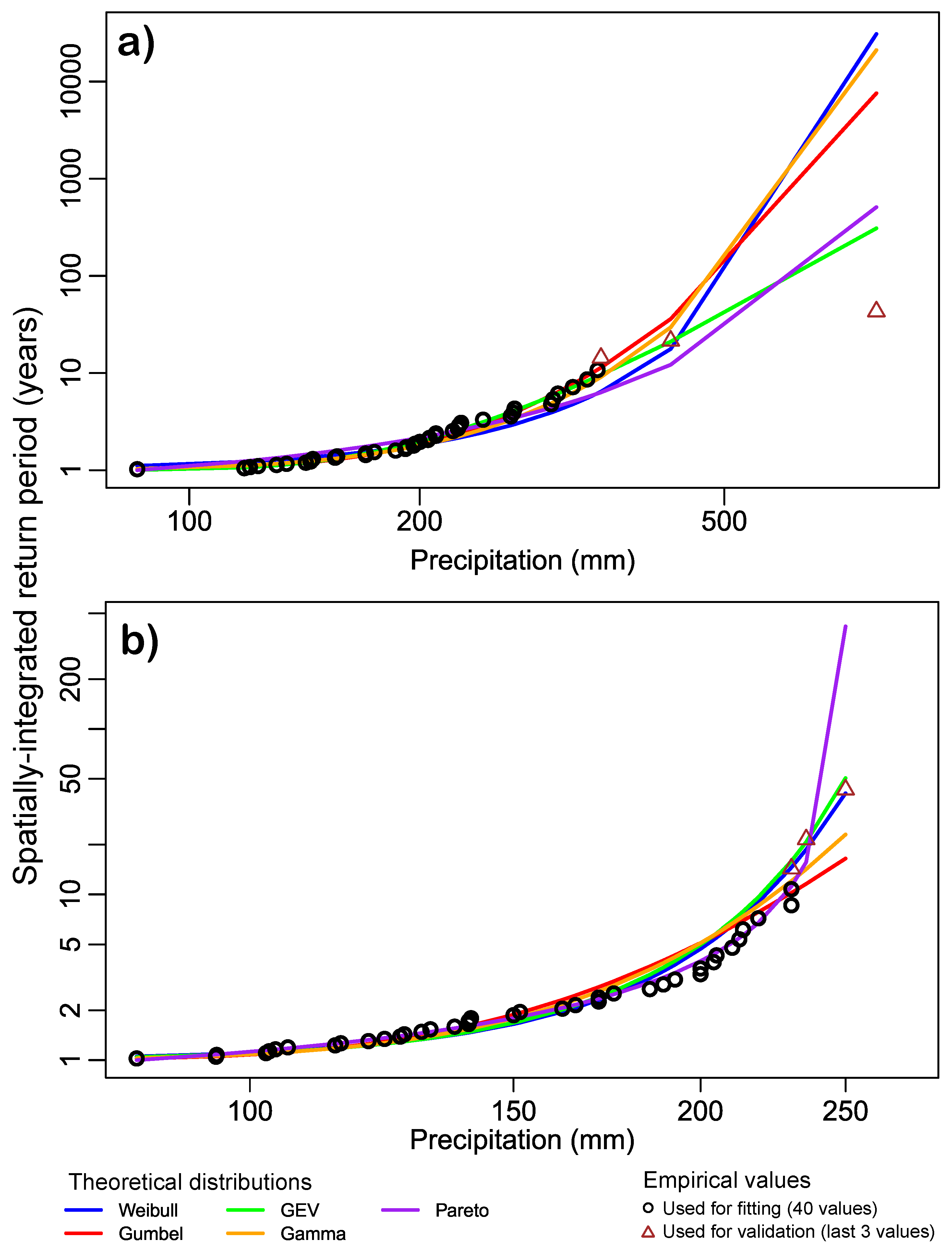
Extreme precipitation poses a major natural hazard in the western Mediterranean, particularly along the Valencia coast, where torrential events recur with significant societal impacts. This study evaluates the feasibility and added value of an explicitly spatial approach for estimating return periods of extreme precipitation in the Júcar and Turia basins, moving beyond traditional point-based or micro-catchment analyses. Our methodology consists of progressive spatial aggregation of time series within a basin to better estimate return periods of exceeding specific catastrophic rainfall thresholds. This technique allows us to compare 10-min rainfall data of a reference station (e.g. Turis, València, 29 October 2024 catastrophe) with long-term annual maxima from 98 stations. Temporal structure is characterized using the fractal--intermittency \( n \)-index, while tail behavior is modeled using several extreme-value distributions (Gumbel, GEV, Weibull, Gamma, and Pareto) and guided by empirical errors. Results show that return periods systematically decrease and stabilize as stations are added, forming a plateau with about 15-20 stations, once the relevant spatial heterogeneity is sampled. The analysis of the precipitation in the 2024 catastrophe highlights the role of time concentration of large amounts over short effective durations. Overall, the results demonstrate that spatially-integrated return-period estimation is operational, physically consistent, and better suited for basin-scale risk assessment than purely point-based approaches.

Keywords: 
;  ;  ;  ;  ;  ;  

1. Introduction

1.1. Context

Extreme precipitation constitutes one of the primary natural hazards in the coastal regions of the western Mediterranean. In particular, the Júcar-Turia system (Spain) is among the most exposed areas in Europe to torrential rainfall episodes, with historical records frequently approaching or exceeding 500 mm in less than 24 hours [1,2]. This hazard arises from quasi--stationary mesoscale convective systems (MCS) as a result of the interaction of: i) a massive supply of warm, moist air from the Mediterranean Sea, ii) an upper-level flux divergency due to the proximity of an isolated depression (DANA or cut-off low), and iii) a complex orography that facilitates an efficient humidity convergence. The confluence of all these factors have driven recurrent catastrophic events in the Júcar-Turia system, mainly in October, including those of 1957 (València), 1982 (Tous), 1987 (Oliva) and the episode of 29 October 2024, which reached 771.8 mm in 24 hours at Turís [3], the second highest 24-hour rainfall total recorded for Spain, after 817.0 mm observed in Oliva on November 3, 1987. Such phenomena lead to devastating flash floods, substantial economic losses, and high mortality rates, underscoring the increasing systemic risk in the region.
In the context of climate change, the intensification of these events has been widely documented [3,4,5,6,7]. Both regional scenarios and observational studies indicate an increasing intensity of rainfall up to +20% in areas that are already highly vulnerable, such as the Valencian coastline [3,8]. Therefore, the study of the temporal structure and statistical recurrence of these episodes is essential for risk management, hydrological planning, and territorial adaptation.

1.2. Episode Recurrence

Numerous studies have addressed the characterization of these phenomena from multiple perspectives. At the synoptic scale, atmospheric patterns associated with extreme events are classified through statistical circulation analysis, confirming the decisive role of blocking configurations and retrograde flows [9,10,11]. On the regional scale, studies such as González-Hidalgo et al. [2] have cataloged a very large number of extraordinary precipitation episodes in the Iberian Peninsula since the beginning of the twentieth century, while Ruiz et al. [12] investigated palaeofloods in the Júcar–Turia system through geomorphological analyzes of alluvial fans and fluvial plains, with at least 10 major floods in five centuries (1571, 1590, 1632, 1776, 1779, 1805, 1864, 1897, 1923, 1949 and 1957). These reconstructions reveal that the actual frequency of catastrophic events far exceeds estimates based solely on instrumental meteorological records [13,14].
An important limitation repeatedly identified in the hydrological literature is the excessive reliance on the classical micro-catchment or point-based approach of Intensity-Duration-Frequency (IDF) curves [15]. Here, micro-catchments are understood as basins of small spatial extent (typically tens to <100 km2), with short concentration times (hours) and rapid hydrological responses strongly controlled by local orography and drainage structure. These units exhibit pronounced spatial and temporal variability in rainfall distribution and runoff generation: the same convective event may produce markedly different maxima at stations separated by only a few kilometers. This spatial heterogeneity is a pattern widely documented in recent studies [16,17].
The point-based (micro-catchment) approach—summarizes hazards using a single representative value per basin—fails to capture this behavior and, critically, the spatial probability of exceedance, i.e., the likelihood that a given threshold is exceeded in at least one subregion of the domain. Recent studies show that extreme precipitation events often display complex spatial dependence structures whose extent and intensity evolve with climate forcing [18], and that neglecting spatial variability leads to systematic underestimation of flood hazard [17]. Moreover, the spatial dependence of extreme rainfall can substantially modify recurrence intervals in a basin, making the analysis of a single station insufficient for regional hazard assessment [19].
Therefore, since basin- or regional-scale hazard depends fundamentally on the joint spatial behavior of extremes, it is necessary to complement (or replace) purely point-based estimates (e.g., Gumbel fitted to a single station or micro-catchment) with explicitly spatial methodologies that integrate information from multiple stations and model the spatial dependence of extremes. The continued use of point-based representations assumes a homogeneous, station-equivalent behavior that is incompatible with the spatial complexity of extreme precipitation processes under current and future climate conditions [20]. As a consequence, the erroneous idea has become widespread that extreme events such as those mentioned above have return periods of hundreds or thousands of years, whereas empirical, geological, and statistical records indicate that they recur several times per century [12,14].

1.3. Rainfall Concentration

In addition, recent studies highlight the need to use new statistical indicators that capture the temporal variability of precipitation beyond simple accumulations. Among them, the fractal intermittency n-index proposed by Monjo [21] stands out as a dimensionless measure that describes the structure of precipitation events according to their degree of concentration and intensity across time scales. Specifically, the maximum precipitation amount ( P t ) expected in a duration of t hours is given by
P t = P 1 h t 1 n P tot = P 1 h t ef 1 n
where P 1 h is the maximum precipitation recorded in 1 hour, and the effective duration t ef is defined when the maximum amount is equal to the total amount. Eq. 1 can be derived from the Maximun Average Intensity (MAI) relationship implemented in empirical IDF curves with power-law behavior [15]. The n-index is a dimensionless indicator that describes precipitation variability on different temporal scales. Its value ranges between 0 and 1, where values close to 0 indicate more uniform–continuous rainfall, whereas values close to 1 indicate highly concentrated–intermittent rainfall, and n = 0.5 denotes a balance between intensity and duration [21].
The n-index approach has been applied in both global and regional analyzes and has proven useful for complementing the hydrological modeling of intense episodes [16,22,23,24,25,26]. Its application is key in climate modeling, allowing a better understanding of rainfall patterns and their impact on water resource management and the prediction of extreme events.
Against this background, the present work proposes an advanced statistical approach to characterize extreme precipitation episodes in the Júcar-Turia system, using a combination of high-resolution data and long-term historical series. The analysis begins with a detailed examination of the event that occurred on 29 October 2024, one of the most devastating in recent decades, which particularly affected the municipality of Turís (Valencia Province).
Through the use of the fractal–intermittency n-index and the estimation of empirical and theoretical return periods through fitting to different probability distributions, the representativeness and frequency of this episode are evaluated within the context of the last decades. Unlike previous studies, the approach adopted here integrates multiple stations within each water basin, allowing the analysis of annual maxima and their aggregated spatial behavior. In addition, a sensitivity analysis is introduced as a function of the number of stations to assess how return periods and fitting errors vary as greater spatial coverage is incorporated.
The article is structured as follows: Section 2 presents the data used and describes the methodological framework, including the calculation of spatially-integrated return periods with sensitivity analysis and the n-index; Section 3 presents the results obtained; while Section 4 discusses their climatic, hydrological, and territorial interpretation, and draws general conclusions to outline future research directions.

2. Materials and Methods

2.1. Observed Data

A total of 98 time series of daily precipitation (1981–2024), recorded in stations located in the Júcar-Turia system, were collected from the Spanish Meteorology Agency (AEMET) database: 58 stations correspond to the Júcar basin and 40 are located in the Turia basin (Figure 1). To analyze the extreme precipitation episode that occurred on 29 October 2024 and severely affected Valencian territory, 10-minute precipitation data recorded by an automatic weather station located in the municipality of Turís were also used (records from 28/10/2024 00:00 h to 31/10/2024 00:00 h, local time).

2.2. Point and Spatially-Integrated Frequency

Point and spatially-integrated return periods were estimated for several reference thresholds of extraordinary episodes, including the 2024 case. Point return periods ( ρ ) represent the expected average time between precipitation (p) events that exceed a certain threshold of pluvial amount (P, our case), intensity, or fluvial avenue, according to the cumulative probability Π ( p P ) of a unique time series ( N = 1 ); that is,
ρ 1 Π ( p > P ) = 1 1 Π ( p P ) .
In contrast, spatially-integrated periods also represent return periods ρ but using N > 1 time series (from stations located nearby), so the probability of exceeding thresholds is significantly higher. Both indicators are used to assess the probability of occurrence of extreme events over a given time span. The longer the return period, the less frequent and more intense the associated event.
The time series used for all subsequent calculations consist of the annual maximum values extracted from a set of N time series (subsequently adding stations); that is, the maximum of the annual maxima is considered to build a synthetic annual time series that integrates all the N stations considered. Distribution fitting was performed using families commonly employed in extreme value theory; Weibull, Gumbel, Generalized Extreme Value (GEV), Gamma, and Pareto distributions were considered [27], as these families are specifically designed to model distribution tails and extreme phenomena. In contrast, central-limit distributions such as the normal distribution are not suitable for describing the probability of occurrence of extreme values due to their rapidly decaying tails. The resulting areal IDF curves were compared to the empirical n-index power law found by Moncho and Caselles [15]:
P t , ρ , N = P t 0 , ρ 0 , N 0 ρ N ρ 0 N 0 m t t 0 1 n ρ 1 / N ,
where m is the scaling parameter, while P t , ρ , N and P t 0 , ρ 0 , N 0 are, respectively, the maximum precipitation amounts recorded in a small area by N and N 0 stations, as expected for a return period ρ and ρ 0 , within an episode of duration t and t 0 . If N = N 0 = 1 , Eq. 3 provides a classical empirical IDF curve as I t , ρ = P t , ρ / t . On the other hand, for N N 0 > 1 statistically-independent stations, Eq. 3 represents an empirical relationship between the spatially-integrated return period ρ and the maximum precipitation amount P t , ρ , N . To analyze the effect of N on the return period ρ , we set the curves of Eq. 3 for constant precipitation thresholds P t , ρ , N = P t 0 , ρ 0 , N 0 , for example, 200 or 500 mm. Here, we assumed that the return period changes as follows:
ρ = ρ min + ( ρ max ρ min ) 1 N λ ( N ) ,
where ρ max is the return period considering only the extremest station, while ρ min is the lowest return period, found when all the stations are used, and λ ( N ) is an independence parameter: Statistically, λ = 1 means that the stations are purely independent (i.e., recovering the ρ 1 / N relationship of Eq. 3 with ρ min = 0 ), while λ = 0 implies that all stations are purely dependent and do not contribute to new extremes. For this study, we considered a reduction of λ from 1 to 0 as N / N 0 increases with respect to a certain N 0 , specifically λ ( N ) exp ( N / N 0 ) .

2.3. Sensitivity Analysis of Episode Recurrence

The fit of the theoretical cumulative distributions was compared with the empirical cumulative function to evaluate which model best reproduces the observed behavior across different ranges (e.g., fitted versus extrapolated). To differentiate between well-sampled and extreme cases, two disjunct ranges of return periods were considered: the fitting range (40 values) and the validation range (3 extremest values). The fitting range includes return periods where multiple observations are available, allowing for robust statistical fitting. In contrast, the validation range corresponds to very large return periods, often represented by only one or two observations. These extreme cases are exceptionally rare, leading to return periods that are extremely high and potentially distant from the true values due to the lack of additional extreme observations. Evaluating the validation range separately helps quantify the uncertainty associated with extrapolating beyond the observed data.
The accuracy of the fitted distributions was quantified using the mean absolute error (MAE) and the root mean square error (RMSE), calculated between the modeled and empirical values of the spatially-integrated return periods. Given a set of K observations (i.e. K annual maxima and their return periods), the errors are defined as:
MAE = 1 K i = 1 K ρ i model ρ i empirical
and
RMSE = 1 K i = 1 K ρ i model ρ i empirical 2 ,
where ρ i model and ρ i empirical are the modeled and observed return periods, respectively. These metrics were calculated separately for the fitting range and the validation range, allowing assessment of model performance in well-sampled versus extreme, poorly-sampled conditions.
The spatial-integration analysis was then conducted by computing the evolution of the return period as stations are progressively added to the analysis, in order to capture a spatial evolution rather than a purely temporal one. Calculations were performed on maximum series derived from different station subsets, with blocks of five stations. For each subset, the different fitting methods were compared in order to select the one with the lowest error.

2.4. Rainfall-Concentration Comparison

To complete the time structure of the obtained IDF curves, a comparison of different extreme precipitation episodes was made together with the data for the 29 October 2024 episode using the fractal–intermittency n-index (Eq. 1). It is calculated from the multifractal analysis of the precipitation series, using a multiplicative cascade approach to assess variability at different scales [21]. The analysis of rainfall concentration was carried out mainly using the n-index.r script and functions_spell.r scripts [28] to compute the n-index and display the results of the case study. For the estimation of return periods, both fitdistrplus and evd libraries were applied [29,30].
For general data processing and analysis, RStudio was used, an integrated development environment for the R programming language that facilitates data manipulation, statistical model development, and result visualization, providing advanced tools for the exploration and analysis of precipitation time series,

3. Results

3.1. Episode Recurrence

For the Júcar basin (Figure 2 a), the best fit is obtained using either the Gumbel or the GEV distribution, although it should be noted that for very high precipitation values none of the methods is able to adequately reproduce the observed maximum. In contrast, for the Turia basin (Figure 2 b), the Pareto distribution appears to provide the best fit to the empirical data, except for the highest precipitation values (validation range), where Weibull or GEV show a better performance. To more precisely assess which fit performs best, fitting errors were calculated with respect to the empirical distribution (Table 1).
After computing the errors, Pareto is identified as the best fit for the Turia basin, except for the values used for validation, for which Weibull provides the best performance. For the Júcar basin, Gumbel exhibits the lowest error across most of the distribution, except for the most extreme values, where GEV better defines the return periods.
Although the analysis was carried out using the best-performing method for each individual case (and even for each subset of stations), overall, GEV produced the lowest average error. Finally, for stations located within the Júcar basin, a GEV fit was applied to all subsets due to the small differences in error in the estimation of the return period compared to the large differences observed in return periods for extreme values. In contrast, for the Turia basin, GEV was the dominant method for the first two station subsets, whereas Weibull was applied to the remaining subsets.
Figure 3. Evolution of the spatially-integrated return periods for Júcar basin (a) and Turia basin (b) according to distinct severity thresholds (four colors). Intervals represent the MAE error of the fitted return periods. Dashed lines represent fitted curves (Eq. 4) with three parameters (Table 2).
Preprints 193180 g003
The results showed that the evolution of the return period follows a power-law decay curve with a final stabilization (Figure 4). This structure is more stable for the Turia basin, as there is less variation between extreme values, while for the Júcar basin the evolution for the highest thresholds (e.g. 400 and 500 mm) is more irregular, as the incorporation of many stations ( > 30 ) with less extreme rainfall reduces the severity. It should also be noted that the evolution of the fitting errors is proportional to the number of stations considered: the greater the number of stations, the larger the uncertainty in the return periods.
For both basins, the five or ten stations that exhibit the highest maxima are those that logically introduce the largest reduction in the estimates of the spatially-integrated return period, with the station that records the highest precipitation maximum in each basin standing out most clearly. Table 2 confirms that a critical number of stations is N 0 9 for Júcar and N 0 3 for Turia, which provides most of the reduction in the return period (from ρ max to ρ min ).
Moreover, if N = N 0 is fixed, Eq. 3 provides a representative areal IDF curve such as
P 1 d a y , ρ = P 1 d a y , 1 y e a r ρ min 1 year m
with scaling parameter m = 0.31 ± 0.02 for Júcar and m = 0.30 ± 0.09 for Turia basin, which reproduces the thresholds ( P 1 d a y , ρ , Table 2) from P 1 d a y , 1 y e a r = 171 ± 8 mm and P 1 d a y , 1 y e a r = 134 ± 10 mm, respectively.

3.2. Rainfall Concentration

For the 2024 catastrophic event, two major precipitation peaks were observed, with the second peak clearly standing out from the first; therefore, the main analysis focuses on this latter segment. An n-index of 0.27 and an effective duration of 4.94 h were calculated, considering that the maximum hourly precipitation reached 170.2 mm and that the maximum accumulated precipitation within the segment corresponding to the largest peak amounted to 620.6 mm (Fig).
The effective duration was also computed considering the entire precipitation time series, while maintaining an n-index of 0.27, as this value best represents the entire series. In this case, the expected duration is 7.3 h. If n is replaced by 0.5 to evaluate the duration that would be required in an “efficient” case for the same total amount of precipitation, an effective duration of 13.3 h is obtained.
To compare with other cases, the n-index and effective duration were estimated according to Eq. 1 and shown in Table 3. The n-index of Turís during the 2024 DANA episode is the second lowest record for extreme precipitation after the Sueca event of 23 September 2008 (326 mm in 3 hours and 144 mm in 1 hour), with n = 0.14 ± 0.01 for an effective duration of 2.9 hours. The difference can be characterized by the spatial scale of the storms. The anchored convective cell of the 2008 episode (horizontal scales of 5–10 km) was four times smaller compared to the quasi-stationary MCS of the 2024 DANA episode (storm focus size of about 20-40 km).
Assuming stationarity (i.e. omitting climate change effects) and taking into account the parameters of Eq. 5 and Table 3 in Eq. 3, total amount (772 mm) of the 29 October 2024 episode in Turís is given by the following curve:
772 mm = ( 171 ± 8 ) mm ρ min 1 year 0.31 t e f 7.3 hours 1 0.27
where the effective duration of the 1-day accumulation was t e f = 7.3 hours. Therefore, the return period of this catastrophe is obtained from Eq. 6 as ρ min = 130 ± 40 years for the Júcar basin, while the threshold of 500 mm has only 33 ± 2 years of return period (Table 2).

4. Discussions and Conclusions

4.1. Spatially-Integrated Return Periods

This work was conceived as a feasibility assessment of an explicitly spatial approach to estimate return periods of extreme precipitation, progressively incorporating stations within each basin (Júcar and Turia). The results confirm that the approach is operational and consistent with probabilistic reasoning: as the number of stations increases, the return period (when at least one station exceeds a given threshold within the domain) decreases up to a certain spatial sample size of about 15-20 stations. Moreover, beyond that sample, the spatially-integrated return period stabilizes into a plateau (i.e., a minimum return period ρ m i n ), because newly added stations no longer contribute annual maxima higher than those previously observed. This decreasing power law (e.g., Eq. 4) is particularly clear in the Turia basin and somewhat more irregular in the Júcar basin for high thresholds, suggesting differences in internal heterogeneity between domains. Overall, the evidence supports the idea that a highly localized anomaly should not inflate regional return periods when the objective is basin-scale hazard and when the metric is correctly defined in spatial terms, so with areal IDF curves. Moreover, the value of the plateau ρ min 33-130 years for catastrophic thresholds (e.g. 500–700 mm/day) is consistent with the observed palaeofloods in the Júcar–Turia system: at least 10 major floods in five centuries [12].
The observed uncertainty of the estimates is also consistent with the spatial variability and the aggregation effects. As stations are added, estimation errors initially increase: expanded spatial coverage introduces heterogeneity (different local regimes), and spatial dependence among series reduces the effective sample size, so uncertainty does not decrease mechanically with the number of stations. Once the regional tail becomes “well sampled”, both return periods and errors tend to stabilize. This interpretation is consistent with the reported pattern that “the probability is proportional to the number of stations”, as well as with the plateau observed in the return period–number of stations relationship for different precipitation thresholds.

4.2. Selection of Theoretical Distributions

Regarding tail modeling, the study documents differences by basin and range. In the Júcar basin, Gumbel exhibits the lowest mean error across the distribution, although GEV better represents the extremes, which is why GEV is used for the spatial station sets in this basin. In the Turia basin, Pareto provides the best overall fit except in the validation range, where Weibull improves performance; for block aggregation, GEV dominates in the first two station sets, while Weibull is applied to the subsequent ones. On the aggregated scale, the GEV yields the lowest mean error, but a case-by-case criterion is adopted, prioritizing the best-performing fit for each station set. This result reinforces two key ideas: (i) the need for adaptive selection of the distribution family depending on the domain and the range considered (observed versus extrapolated), and (ii) the importance of reporting uncertainty bands specific to the fitted model used in each range.
Finally, several limitations and avenues for improvement, already implicit in the study design, should be acknowledged: (a) the use of annual maxima facilitates comparability but may underutilise POT (peaks-over-threshold) information and seasonality; (b) spatial dependence among stations suggests the use of resampling techniques or spatial extreme-value frameworks to better quantify uncertainty; and (c) the order in which stations are incorporated could be explored through sensitivity analyses (e.g., starting with stations exhibiting the highest maxima or based on climatic proximity criteria). Nevertheless, the primary objective is fulfilled: the proposed spatial method is viable, behaves as expected, and produces stable and traceable return period estimates once the relevant climatological heterogeneity of each basin is adequately covered. In any case, the annual maximum approach is enough for the areal IDF analysis. More sophisticated options such as three- and four-parametric distributions would be more adequate for daily precipitation modeling from entire time series [27].

4.3. Episode Time Structure

The use of the fractal–intermittency n-index provides physical–statistical context to the analysed episodes (e.g., the 2024 DANA event in Turís), allowing comparisons of temporal efficiency and intermittency against historical cases (such as the 2008 event), and linking temporal structure to accumulated severity. The IDF combination of n-index, annual maxima, and tail fitting offers a consistent interpretation of hazard: episodes with values close to n 0.3 0.5 (more efficient rainfall) can concentrate large amounts within relatively short effective windows, which is highly relevant for threshold definition and for the interpretation of regional maxima employed in spatial return period estimation.

4.4. Final Recommendation

From an operational perspective, the study supports three recommendations: (i) Explicitly define the spatially-integrated return period (e.g., “at least one station”, k-of-N, or areal average) according to the management question, as values are not interchangeable across definitions. (ii) When aggregating stations in blocks (here, groups of five), jointly assess return periods and errors, and stop aggregation when changes in return periods fall below a practical threshold (e.g., < 5 %) and the error reaches its plateau. (iii) Accompany each return period estimate with its associated uncertainty and with the fitting method selected for that specific station set and range, in line with the distribution-specific error evidence for each basin. (iv) Analyze the dependence of the spatially-integrated return period and the number of stations considered using an empirical relationship (e.g. Eq. 4), and finally obtain a better estimate of the annual maxima ( P 1 d a y , 1 y e a r , Eq. 5) and its corresponding IDF curve (e.g. Eq. 6).

Author Contributions

Conceptualization, R.M.; methodology, R.M.; software, P.P-d-G.; validation, P.P-d-G. and R.M.; formal analysis, P.P-d-G. and R.M.; investigation, P.P-d-G. and R.M.; resources, P.P-d-G.; data curation, P.P-d-G.; writing—original draft preparation, P.P-d-G.; writing—review and editing, R.M.; visualization, P.P-d-G. and R.M.; supervision, R.M.; project administration, R.M.; funding acquisition, R.M. All authors have read and agreed to the published version of the manuscript.

Funding

This research received no external funding

Data Availability Statement

Data will be made available on request.

Acknowledgments

We would like to thank the Darío Redolat and David Rodríguez for reviewing our paper.

Conflicts of Interest

The authors declare no conflicts of interest.

References

  1. Gonzalez, S.; Bech, J. Extreme point rainfall temporal scaling: a long term (1805–2014) regional and seasonal analysis in Spain. Intemational Journal of Climatology 2017, 37, 5068–5079. [Google Scholar] [CrossRef]
  2. Gonzalez-Hidalgo, J.C.; Beguería, S.; Peña-Angulo, D.; Blanco, V.T. Catalogue and Analysis of Extraordinary Precipitation Events in the Spanish Mainland, 1916–2022. International Journal of Climatology 2025, 45, e8785. [Google Scholar] [CrossRef]
  3. Barriopedro, D.; Jiménez-Esteve, B.; Collazo, S.; Garrido-Perez, J.M.; Johnson, J.E.; García-Herrera, R. A Multimethod Attribution Analysis of Spain’s 2024 Extreme Precipitation Event. Bulletin of the American Meteorological Society 2025, 106, E2440–E2460. [Google Scholar] [CrossRef]
  4. L, A.; L, F.; D.B., G. Increasing flood risk under climate change: a pan-European assessment of the benefits of four adaptation strategies. CLIMATIC CHANGE 2016, 136, 507–521. [Google Scholar] [CrossRef]
  5. Alfieri, L.; Dottori, F.; Betts, R.; Salamon, P.; Feyen, L. Multi-Model Projections of River Flood Risk in Europe under Global Warming. Climate 2018, 6. [Google Scholar] [CrossRef]
  6. Kotz, M.; Lange, S.; Wenz, L.; Levermann, A. Constraining the Pattern and Magnitude of Projected Extreme Precipitation Change in a Multimodel Ensemble. Journal of Climate 2024, 37, 97–111. [Google Scholar] [CrossRef]
  7. Zhang, W.; Zhou, T.; Wu, P. Anthropogenic amplification of precipitation variability over the past century. Science 2024, 385, 427–432. [Google Scholar] [CrossRef] [PubMed]
  8. Green, A.C.; Fowler, H.J.; Blenkinsop, S.; et al. Precipitation extremes in 2024. Nature Reviews Earth & Environment 2025, 6, 243–245. [Google Scholar] [CrossRef]
  9. Dayan, U.; Nissen, K.; Ulbrich, U. Review Article: Atmospheric conditions inducing extreme precipitation over the eastern and western Mediterranean. Natural Hazards and Earth System Sciences 2015, 15, 2525–2544. [Google Scholar] [CrossRef]
  10. Mastrantonas, N.; Herrera-Lormendez, P.; Magnusson, L.; Pappenberger, F.; Matschullat, J. Extreme precipitation events in the Mediterranean: Spatiotemporal characteristics and connection to large-scale atmospheric flow patterns. International Journal of Climatology 2021, 41, 2710–2728. [Google Scholar] [CrossRef]
  11. Vicente-Serrano, S.M.; Garrido-Perez, J.M.; Fernández-Álvarez, J.C.; et al. Characteristics of widespread extreme precipitation events in Peninsular Spain and the Balearic Islands: spatio-temporal dynamics and driving mechanisms. Climate Dynamics 2025, 63, 340. [Google Scholar] [CrossRef]
  12. Ruiz, J.M.; Carmona, P.; Pérez Cueva, A. Flood frequency and seasonality of the Jucar and Turia Mediterranean rivers (Spain) during the “Little Ice Age”. Méditerranée 2014. [Google Scholar] [CrossRef]
  13. Benito, G.; Díez-Herrero, A. Chapter 3 - Palaeoflood Hydrology: Reconstructing Rare Events and Extreme Flood Discharges. Hydro-Meteorological Hazards, Risks and Disasters 2015, 65–104. [Google Scholar] [CrossRef]
  14. Wilhelm, B.; Ballesteros-Cánovas, J.A.; Macdonald, N.; Toonen, W.H.; Baker, V.; Barriendos, M.; Benito, G.; Brauer, A.; Corella, J.P.; Denniston, R.; et al. Interpreting historical, botanical, and geological evidence to aid preparations for future floods. 2019. [Google Scholar] [CrossRef]
  15. Moncho, R.; Caselles, V. Potential distribution of extreme rainfall in the Basque Country. Tethys 2011, 8, 3–12. [Google Scholar] [CrossRef]
  16. Gonzalez, S.; Bech, J. Extreme point rainfall temporal scaling: a long term (1805–2014) regional and seasonal analysis in Spain. International Journal of Climatology 2017, 37, 5068–5079. [Google Scholar] [CrossRef]
  17. Xu, H.; Guan, Y.; Li, P.; et al. Quantifying the Impact of Rainfall Spatial Heterogeneity and Patterns on Urban Flooding by Integrating Machine Learning Algorithm and Hydrodynamic–Hydrological Modeling. Water Resources Management 2026, 40, 31. [Google Scholar] [CrossRef]
  18. Zhong, P.; Brunner, M.; Opitz, T.; Huser, R. Spatial Modeling and Future Projection of Extreme Precipitation Extents. Journal of the American Statistical Association 2025, 120, 80–95. [Google Scholar] [CrossRef]
  19. Zhang, Q.T.; Qian, J.L.; Jiang, X.J.; Wu, Y.X.; Yu, P.B. Spatial Dependence of Conditional Recurrence Periods for Extreme Rainfall in the Qiantang River Basin: Implications for Sustainable Regional Disaster Risk Governance. Sustainability 2025, 17. [Google Scholar] [CrossRef]
  20. Fraga, I.; Cea, L.; Puertas, J. Effect of rainfall uncertainty on the performance of physically based rainfall–runoff models. Hydrological Processes 2019, 33, 160–173. [Google Scholar] [CrossRef]
  21. Monjo, R. Measure of rainfall time structure using the dimensionless n-index. Clim. Res. 2016, 67, 71–86. [Google Scholar] [CrossRef]
  22. Monjo, R.; Martin-Vide, J. Daily precipitation concentration around the world according to several indices. International Journal of Climatology 2016, 36, 3828–3838. [Google Scholar] [CrossRef]
  23. Agbazo, M.N.; Adéchinan, J.A.; N’gobi, G.K.; Bessou, J. Analysis and Predictability of Dry Spell Lengths Observed in Synoptic Stations of Benin Republic (West Africa). American Journal of Climate Change 2021, 10. [Google Scholar] [CrossRef]
  24. Monjo, R.; Locatelli, L.; Milligan, J.; Torres, L.; Velasco, M.; Gaitan, E.; Portoles, J.; Redolat, D.; Russo, B.; Ribalaygua, J. Estimation of future extreme rainfall in Barcelona (Spain) under monofractal hypothesis. Int. J. Climatol. 2023, 163, 4047–4068. [Google Scholar] [CrossRef]
  25. Gacon, B.; Santuy, D.; Redolat, D. Temporal Distribution of Extreme Precipitation in Barcelona (Spain) under Multi-Fractal n-Index with Breaking Point. Atmosphere 2024, 15. [Google Scholar] [CrossRef]
  26. Collar, N.M.; Moody, J.A.; Ebel, B.A. Rainfall as a driver of post-wildfire flooding and debris flows: A review and synthesis. Earth-Science Reviews 2025, 260, 104990. [Google Scholar] [CrossRef]
  27. Monjo, R.; Gaitán, E.; Pórtoles, J.; Ribalaygua, J.; Torres, L. Changes in extreme precipitation over Spain using statistical downscaling of CMIP5 projections. International Journal of Climatology 2016, 36, 757–769. Available online: https://rmets.onlinelibrary.wiley.com/doi/pdf/10.1002/joc.4380. [CrossRef]
  28. Monjo, R.; Royé, D.; Martin-Vide, J. Meteorological drought lacunarity around the world and its classification. Earth Syst. Sci. Data 2020, 12, 741–752. [Google Scholar] [CrossRef]
  29. Delignette-Muller, M.L.; Dutang, C. fitdistrplus: An R Package for Fitting Distributions. Journal of Statistical Software 2015, 64, 1–34. [Google Scholar] [CrossRef]
  30. Stephenson, A.G. evd: Extreme Value Distributions. R News 2002, 2, 31–32. [Google Scholar]
Figure 1. Geographical location of the Júcar River Basin District with the Júcar and Turia basins and their corresponding maximum-recording stations. The map shows the location of the 98 stations included in the analysis, marked with different colors to distinguish those presenting the highest observed maxima in each basin.
Preprints 193180 g001
Figure 2. Comparison of the probability distributions of extreme precipitation for the set of all the stations in the Júcar river basin (a) and in the Turia river basin (b). Empirical values are represented in black circles, while the theoretical fits are sketched in colored curves.
Preprints 193180 g002
Figure 4. Characterization of the catastrophic rainfall recorded in Turís (València) on 29 October 2029, during the morning (first row) and especially during the afternoon (second row): 10-min hyetograph (first column), maximum accumulation curves P t (second column), and maximum intensity curves P t / t curve (third column) from the n-index approach (Eq. 1). Dashed lines on the second column symbolize ideal accumulation of maximum precipitation according to several n-index values. The red curves are theoretical fits with standard-error uncertainty.
Preprints 193180 g004
Table 1. Errors of return periods (years) for fitted distributions (top) and for their validation ranges (bottom) for all the stattions of the Júcar and Turia basins.
Júcar basin Turia basin
Range Distribution MAE RMSE MAE RMSE
Fitting Weibull 0.80 1.67 0.65 1.31
Gumbel 0.26 0.56 0.59 1.01
GEV 0.28 0.82 0.84 1.68
Gamma 0.44 0.98 0.65 1.04
Pareto 0.72 1.62 0.28 0.68
Validation Weibull Pred. 15400 22000 2.5 2.5
Gumbel Pred. 3800 5300 18 20
GEV Pred. 133 188 4.1 5.3
Gamma Pred. 10500 14900 13.6 15.0
Pareto Pred. 240 330 190 270
Table 2. Estimated parameters ( ρ min , ρ max , N 0 ) with their standard errors for the Júcar and Turia basins according to Eq. 4.
Threshold [ P 1 d a y , ρ ] ρ min (years) ρ max (years) N 0
Júcar 200 mm 1.81 ± 0.13 11.58 ± 0.36 9.30 ± 1.21
300 mm 5.23 ± 0.37 28.94 ± 1.05 9.45 ± 1.45
400 mm 14.14 ± 0.94 56.26 ± 2.70 8.54 ± 1.95
500 mm 33.20 ± 2.50 94.28 ± 7.50 6.91 ± 3.24
Turia 120 mm 1.00 ± 0.03 7.20 ± 0.09 2.77 ± 0.31
150 mm 1.19 ± 0.07 13.12 ± 0.19 3.27 ± 0.34
180 mm 2.02 ± 0.11 21.90 ± 0.30 3.51 ± 0.32
210 mm 5.34 ± 0.15 34.12 ± 0.41 3.04 ± 0.30
Table 3. Comparison of the 2024 episode features (Eq. 1) with recent historical episodes.
Date Station Basin P 1 h (mm) n P tot (mm) t ef (hours)
20/10/1982 Casas del Baró Júcar 140 0.37 975 * 21.8
03/11/1987 Gandia Serpis 154 0.42 1000 * 26.3
03/11/1987 Oliva Serpis 150 0.41 817 17.7
22/10/2000 Carlet Júcar 60 0.35 532 28.7
12/10/2007 Alcalalí Xaló–Gorgos 90 0.35 440 11.5
23/09/2008 Sueca Júcar 142 0.14 350 2.9
29/10/2024 Turís Turia-Jucar 180 0.27 772 7.3
* Estimation according to proxy data and testimonies.
Disclaimer/Publisher’s Note: The statements, opinions and data contained in all publications are solely those of the individual author(s) and contributor(s) and not of MDPI and/or the editor(s). MDPI and/or the editor(s) disclaim responsibility for any injury to people or property resulting from any ideas, methods, instructions or products referred to in the content.
Copyright: This open access article is published under a Creative Commons CC BY 4.0 license, which permit the free download, distribution, and reuse, provided that the author and preprint are cited in any reuse.
Prerpints.org logo

Preprints.org is a free preprint server supported by MDPI in Basel, Switzerland.

Subscribe

Disclaimer

Terms of Use

Privacy Policy

Privacy Settings

© 2026 MDPI (Basel, Switzerland) unless otherwise stated