Submitted:
15 September 2025
Posted:
16 September 2025
You are already at the latest version
Abstract
This study proposes a bivariate distribution with Exponentiated Gumbel (BEG) marginals to estimate return levels of annual maximum daily rainfall in Mexico. A dataset of 181 gauging stations from two contrasting climatic regions was analyzed, and the BEG model was compared against the Generalized Extreme Value (GEV), Gumbel (EVI), and Exponentiated Gumbel (EG) distributions. Parameters were estimated using the maximum likelihood method. Goodness-of-fit assessment based on AICc and BIC indicated that 71.8% of the samples were better described by the BEG model than by the univariate alternatives. Moreover, differences in return level estimates became more pronounced at higher non-exceedance probabilities. These results suggest that the BEG distribution provides a robust and reliable tool for the frequency analysis of extreme rainfall.
Keywords:
extreme rainfall
; frequency analysis
; bivariate distribution
; exponentiated gumbel
; maximum likelihood estimation: AICc and BIC
; return levels
1. Introduction
[1] highlighted that variations in the hydrological cycle have profound impacts on human activities, including an increased risk of flooding as well as the occurrence and severity of droughts. Floods are among the most damaging natural hazards worldwide, and their impacts have intensified due to factors such as irregular human settlements near rivers, deforestation, and continuous land-use changes.
Mexico is especially vulnerable to hydrometeorological events that cause widespread damage across its territory. Between 2007 and 2020, heavy rains, floods, and tropical cyclones affected 27.8 million people, resulting in 1,173 fatalities and economic losses exceeding 24.6 billion USD [2]. Analyses of rainfall patterns in Mexico [3,4] indicate that floods caused by extreme rainfall events are likely to become more frequent and intense in the future. Given the potential consequences of underestimating or overestimating rainfall quantiles—ranging from hydraulic structure failure to unnecessarily inflated construction costs—reliable statistical tools are essential for estimating their magnitude and frequency.
Numerous at-site and regional rainfall frequency analyses have been conducted worldwide, and results consistently demonstrate that no single distribution universally fits annual maximum daily rainfall (AMDR) data. Although the Gumbel distribution (EVI) is widely applied, studies such as [5] in Egypt have shown that it is not always appropriate, while in other regions it has been identified as the most suitable model [6,7,8,9,10,11,12,13,14,15].
In Italy, [16] analyzed AMDR records from 297 gauging stations and found that the Fréchet distribution (EVIII) provided the best fit. Their study also revealed significant differences in return periods and return levels compared to results from EVI, reversed Weibull (EVII), Pareto, Lognormal, and Gamma distributions, echoing earlier findings by [17,18]. The EVI, EVII, and EVIII distributions are all special cases of the Generalized Extreme Value (GEV) distribution, which has often been identified as the best-fitting model for AMDR samples in multiple regions [19,20,21,22,23,24,25,26,27,28]. Similarly, the Log-Pearson Type III (LPIII) distribution has also proven effective in modeling AMDR series [29,30,31,32,33,34].
In recent years, the Exponentiated Gumbel (EG) distribution was proposed by [35], who demonstrated its improved performance in climate modeling compared to the EVI and GEV distributions. [36] applied EG, exponentiated Weibull (EW), exponentiated Fréchet (EF), and their mixed forms to AMDR series from 19 Mexican stations, showing that exponentiated and mixed exponentiated distributions provide flexible and reliable alternatives for modeling extreme rainfall. More recently, [37] compared the Gumbel and EG distributions, concluding—based on AIC and BIC criteria—that EG offered a more flexible fit for hydrological datasets, corroborating earlier findings by [35].
Regional frequency analysis has also emerged as a practical approach to reduce uncertainties associated with short or incomplete rainfall records at gauged sites. In this context, multivariate joint estimation models have proven valuable, as they enhance the estimation of marginal distribution parameters and improve regional at-site estimates of return levels by incorporating information from neighboring sites within homogeneous regions. Bivariate approaches have shown promise in flood frequency analysis [38,39,40,41,42,43,44,45,46,47].
In this study, a bivariate distribution with Exponentiated Gumbel marginals is proposed to improve the estimation of marginal parameters and corresponding quantiles. The performance of this model is compared with that of univariate probability distributions, namely GEV, EVI, and EG.
2. Materials and Methods
2.1. Study Area
Mexico is characterized by a summer–rainy and winter–dry regime, except in the northwest. Annual precipitation ranges from <500 mm in the north and northwest to >2,000 mm in the humid south and southeast. Two states that illustrate this climatic contrast are Coahuila, in northern Mexico, and Tabasco, in the southeast (Figure 1).
Coahuila (151,563 km²) has a semi-warm summer and cold winter climate, with a mean annual temperature of 20 °C (min. 4 °C, max. 30 °C). Rainfall is scarce, averaging ~400 mm yr⁻¹, concentrated in summer. Maximum daily rainfall varies between 11.3 and 453 mm. Recent extreme events have produced floods affecting Torreon, Monclova, and Piedras Negras.
Tabasco (25,267 km²) is predominantly warm-humid, with abundant summer rains (75.97%), year-round humid conditions (19.64%), and sub-humid summer rains (4.39%). The mean annual temperature is 27 °C (min. 18.5 °C, max. 36 °C). Rainfall occurs throughout the year, peaks from June to October, and averages 2,550 mm yr⁻¹. Maximum daily rainfall ranges from 38.8 to 816.9 mm.
2.2. Delineation of Homogeneous Regions
The joint parameter estimation model requires that all samples belong to the same homogeneous region. In this study, regions were delineated using the coefficient of variation (Cv) as the measure of comparability among stations.
In the first stage, three initial zones were identified by setting confidence limits defined as the mean Cv ± one standard deviation. At this stage, most stations were concentrated in region 2 (Figure 2), leaving only the stations in regions 1 and 3 distinctly separated.
In the second stage, the stations within region 2 were reclassified by recalculating new confidence limits and repeating the same procedure. This subdivision resulted in four regions (1, 2, 4, and 5) (Figure 3).
The process was repeated iteratively, each time focusing on the stations remaining in the central region (closer to the mean Cv value). In this case, region 3 was progressively subdivided until a sufficient distribution of stations across regions was achieved. After the final iteration, seven homogeneous regions were identified (Figure 4).
It is important to note that the total number of stages required depends on the number of stations analyzed, since the central group—located around the mean Cv—will ultimately determine how many subdivisions are necessary to achieve adequately homogeneous regions.
2.3. Univariate Distributions
a. GEV distribution
The cumulative distribution function is [49]:
where are the location, scale, and shape parameters, respectively.
And
The log-likelihood for the GEV distribution is:
The quantile corresponding to a given return period T is:
b. EVI (Gumbel) distribution
where are the location and scale parameters
c. Exponentiated Gumbel distribution (EG) [50].
2.4. Biexponentiated Gumbel Distribution (BEG)
As already mentioned, multivariate extreme value distributions have shown to be a reliable option for fitting hydrological variables. [51] compared the mixed and logistic bivariate models and concluded that the logistic model (LM) is the best option in flood frequency analysis.
The LM is [52]:
where x and y denote the extreme events gauged in a couple of neighboring sites.
and
The bivariate likelihood function is:
The log-likelihood function is:
The expression (16) is used when both samples share a common length of record, however, the general form for considering different sizes is [53]:
Marginals F(x) and F(y) are proposed to be EG distributions. The BEG log-likelihood function to maximize in the parameter estimation procedure is:
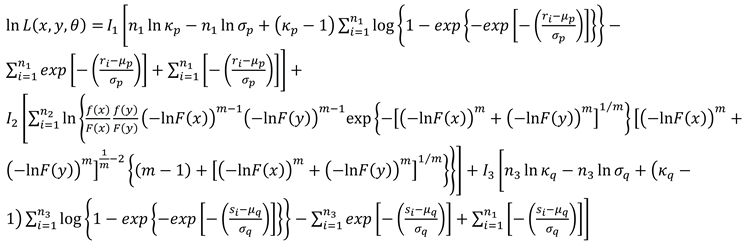 where x and y are the variables in the common period (CP) with length , r denotes to the variable x or y with length before the CP, s is the variable x or y with length after the CP; if if for j = 1, 2, 3; p =1 and q = 1 if r or s represent to variable x; p = 2 and q = 2 if r or s characterize to variable y, and
The Rosenbrock optimization algorithm for constrained variables [54] was selected for estimating the univariate and bivariate parameters by the direct maximization of equations (3), (7), (11), and (18).
2.5. Selection of Best Fit
The selection of fit between the Empirical and Theoretical distribution of the AMDR was based on the AICc and BIC goodness of fit tests.
The AIC was proposed by Akaike [55]:
while the BIC is [56]:
where represents the log-likelihood of empirical distribution, p the number of maximum-likelihood estimates of the parameters, and n the length of record.
Distribution having least value of AICc, or BIC is considered as best model.
2.6. Reliability of Estimated Quantiles
It is very important to evaluate whether the BEG distribution provides more accurate and reliable quantile estimates than traditional univariate approaches. This evaluation is essential in hydrological frequency analysis, since underestimation of quantiles can increase the risk of hydraulic structure failure, while overestimation may result in unnecessarily high construction costs. To assess reliability, quantile estimates obtained from the BEG model were compared with those from univariate distributions using two statistical criteria: bias (BIAS) and mean squared error (MSE). This framework allowed us to determine not only the accuracy of the estimated quantiles but also the extent to which the joint estimation procedure enhances the transfer of information across sites, thereby improving the robustness of extreme rainfall frequency analysis.
To formalize this evaluation, the reliability of estimated quantiles was expressed in terms of bias and mean squared error, which are defined as follows:
Let be the quantile to be computed by using the BEG distribution:
For the number of simulated samples “ ”
And
When estimating quantiles is desirable to have unbiased and minimum MSE estimators.
3. Results
A procedure of data generation was performed to show if the quantiles obtained through of the bivariate joint estimation of parameters are more reliable with those obtained by its univariate counterpart.
For the EG distribution, data were generated using population parameters , and with sample sizes n = 10, 20 and 50. A total of 1,000 simulated samples were considered for each n.
For the BEG distribution, quantiles were obtained by combining samples with sizes n1-n2: 10-10, 10-20, 20-20, 20-50, 50-50 and 50-100. Comparisons were performed for non-exceedance probabilities of 0.50, 0.80, 0.90. 095 0.98 and 0.99. The associated site has population parameters , and .
Results (Table 3 and Table 4) indicate that as increased relative to , both BIAS and MSE of the shorter series decreased. This demonstrates an effective transfer of information when parameters are jointly estimated, supporting the conclusion that quantiles computed using the BEG distribution are more reliable than those obtained from the univariate case.
The rain gauge stations in Coahuila and Tabasco were classified into homogeneous regions by applying the delineation procedure previously described. This methodological approach yielded nine regions in Coahuila (Table 5) and seven regions in Tabasco (Table 6), ensuring consistency with the adopted regionalization framework.
The analysis of the Coahuila dataset considered all possible pairwise station combinations within each homogeneous region to evaluate the dependence structure of extreme rainfall. Table 7 and Table 8 illustrate representative examples for selected stations, showing the BEG model combinations applied (Table 7) and the corresponding return level estimates (Table 8). When extended to the complete set of stations, the procedure enabled a systematic assessment of return levels using the BEG framework. For comparison, alternative univariate models—Gumbel, Generalized Extreme Value (GEV), and Exponentiated Gumbel—were also fitted to the same stations, and the resulting return levels were ranked according to goodness-of-fit statistics, including the Akaike Information Criterion (AIC), and Bayesian Information Criterion (BIC) (Table 9). Notably, in 65% of the stations in Coahuila the best fit was achieved with the BEG distribution, highlighting its reliability for modeling extreme rainfall in this region.
A similar procedure was applied in Tabasco, where all possible station pairs within each homogeneous region were analyzed. Table 10 presents the parameters obtained for the best BEG combination at each station. Return levels derived from the BEG distribution were then compared with those obtained from alternative univariate models (Gumbel, GEV, and Exponentiated Gumbel), and the results were ranked according to statistical criteria (AIC and BIC) (Table 11). In this case, 81% of the stations achieved the best fit with the BEG distribution, confirming the robustness of this approach under the markedly different climatic conditions of southeastern Mexico.
Together, these results demonstrate that the BEG distribution consistently outperforms classical models, providing the best fit in both the arid to semi-arid conditions of Coahuila and the humid tropical environment of Tabasco. This consistency across regions and evaluation metrics underscores the versatility of the BEG framework for regional frequency analysis in contrasting hydroclimatic settings.
4. Discussion
The results obtained in Coahuila and Tabasco demonstrate the advantages of adopting flexible probability models such as the Bivariate Exponentiated Gumbel (BEG) distribution for extreme rainfall analysis. In both regions, the BEG framework provided the best fit for a majority of stations—65% in Coahuila and 81% in Tabasco—when compared to the classical Gumbel, Generalized Extreme Value (GEV), and Exponentiated Gumbel distributions. This superior performance, confirmed by goodness-of-fit criteria including AIC and BIC, highlights the ability of the BEG model to capture the dependence structure of extreme events more effectively than univariate alternatives.
The simulation experiments reinforce this conclusion. By jointly estimating parameters across paired samples, the BEG approach significantly reduced bias and mean squared error in quantile estimation, particularly as one sample length increased relative to the other. This result demonstrates the effective transfer of information between series, a feature that is especially relevant in hydrological contexts where records are often short, fragmented, or incomplete. In contrast, univariate models produced higher estimation errors under identical conditions, confirming the greater robustness of BEG.
An important aspect of these findings is the consistency of the BEG performance across contrasting climatic contexts. In Coahuila, a predominantly arid to semi-arid region, rainfall extremes are generally short-lived and spatially heterogeneous, which complicates regionalization and frequency analysis. Conversely, Tabasco is located in a humid tropical environment where rainfall extremes are often more spatially extensive and influenced by large-scale atmospheric dynamics. Despite these marked hydroclimatic differences, the BEG distribution consistently outperformed traditional models, underscoring its robustness and adaptability.
The systematic evaluation of all possible station pairs within homogeneous regions further strengthens the validity of the results. This approach ensures that spatial dependence is explicitly considered, rather than assuming independence between stations—a limitation common in univariate frequency analysis. The strong performance of the BEG distribution suggests that bivariate or multivariate models may be more appropriate for regions with high spatial variability, particularly where water resource planning and hydraulic design require accurate estimation of joint extremes.
From a practical perspective, the improved fit obtained with the BEG distribution has direct implications for risk management and infrastructure design. Underestimation of return levels, especially for long return periods, can lead to inadequate sizing of hydraulic structures and increased vulnerability to extreme events. By providing more reliable estimates, the BEG framework contributes to reducing uncertainty in hydrological design, supporting more resilient adaptation strategies in the face of climate variability and change.
Finally, these results align with recent studies emphasizing the importance of moving beyond stationary univariate models in hydrology. The incorporation of flexible, bivariate approaches not only improves statistical performance but also offers a more realistic representation of rainfall extremes, particularly in regions with complex climatic dynamics. The outcomes from Coahuila and Tabasco therefore provide empirical evidence supporting the broader adoption of BEG-based regional frequency analysis in Mexico and comparable hydroclimatic contexts.
5. Conclusions
This study applied the Bivariate Exponentiated Gumbel (BEG) distribution to extreme rainfall analysis in Coahuila and Tabasco, two Mexican states with contrasting climatic conditions. The main conclusions are as follows:
Across the stations analyzed, the BEG distribution provided the best fit in 65% of the cases in Coahuila and 81% in Tabasco, outperforming classical alternatives such as the Gumbel, Generalized Extreme Value (GEV), and Exponentiated Gumbel distributions. This performance was consistently confirmed by statistical indicators including AIC and BIC.
Simulation experiments showed that BEG reduced bias and mean squared error when estimating quantiles, especially for short or heterogeneous samples. The joint estimation of parameters allowed effective transfer of information, resulting in more reliable quantiles than those obtained from univariate approaches.
The BEG model demonstrated strong adaptability in both arid to semi-arid conditions (Coahuila) and humid tropical conditions (Tabasco), underscoring its versatility as a tool for regional frequency analysis of extreme rainfall.
The systematic evaluation of all possible pairwise station combinations within homogeneous regions captured spatial dependence more effectively than univariate models. This methodological strength enhances the reliability of rainfall return level estimates, particularly for long return periods.
The improved accuracy of return level estimates obtained with the BEG distribution can reduce underestimation of design events, thereby contributing to safer and more resilient hydraulic infrastructure, as well as supporting climate adaptation planning in water management.
In summary, the BEG distribution proves to be a reliable and flexible alternative for regional extreme rainfall analysis in Mexico. Its demonstrated robustness suggests that it can be extended to other regions with similar hydroclimatic variability, providing a valuable tool for both scientific research and applied hydrological practice. Future research should explore the application of the BEG model under non-stationary conditions, test its performance in multivariate settings that include variables such as streamflow or temperature, and assess its potential for integration into climate change impact studies.
Data Availability Statement
Data will be made available at a reasonable request. Note: Please confirm or update DAS at revision which version we should follow next. DAS type which you selected in the system as follow: Data available in a publicly accessible repository; The original data presented in the study are openly available in [repository name, e.g., FigShare] at [DOI/URL] or [reference/accession number]. Or select an alternative template from the options available through the following link: https://www.mdpi.com/ethics#_bookmark21.
Conflicts of Interest
The author declares no conflicts of interest.
Abbreviations
The following abbreviations are used in this manuscript:
| BEV | Bivariate Extreme Value Distribution |
| FFA | Flood Frequency Analysis |
| GEV | Generalized Extreme Value |
| R | Homogeneous Region |
| T | Return Period |
References
- Held, I., and B. Soden, 2006: Robust responses of the hydrological cycle to global warming. J. Clim., 19:5686-5699. [CrossRef]
- CENAPRED, 2021: Impacto Socioeconómico de los principales desastres ocurridos en la República Mexicana. Centro Nacional de Prevención de Desastres. Versiones del 2007 al 2020. Secretaria de Seguridad y Protección Ciudadana. Gobierno de México. http://www.cenapred.unam.mx/PublicacionesWebGobMX/buscar_buscaSubcategoria.action.
- Jáuregui, E., 2000: El Clima de la Ciudad de México. Instituto de Geografía, UNAM and Plaza y Valdés Editores. 131 p.
- Peralta-Hernández, A., Balling, R. and Barba-Martínez, L., 2009: Comparative analysis of indices of extreme rainfall events: Variations and trends from southern México. Atmosfera, 22(2): 219-228.
- Gado, T., Salama, A., and B. Zeidan, 2021: Selection of the best probability models for daily annual maximum rainfalls in Egypt. Theor. Appl. Climatol., 144:1267-1284. [CrossRef]
- Melice, J-L., and Reason, Ch., 2007: Return period of extreme rainfall at George, South Africa. South Afr. J. Sci., 103: 499-501.
- Nadarajah, S. and D. Choi, 2007: Maximum daily rainfall in South Korea. J Earth Syst. Sci., 116(4): 311-320. [CrossRef]
- Momin, U., Kulkarni, P., Horaginamani, M., Ravichandran, M., Patel, A., and H. Kousai, 2011: Consecutive days maximum rainfall analysis by Gumbel´s extreme value distribution for southern Telangana. Ind. J. Nat. Sci., 2(7): 408-412.
- Chifurira, R., and D. Chikobvu, 2014: Modelling extreme maximum annual rainfall for Zimbabwe. Proceedings of the 56th Annual Conference of the South African Statistical Association. January 2014. 9-16.
- Manzano-Agugliaro, F., Zapata-Sierra, A., and J. Rubi-Maldonado, 2014: Assessment of obtaining IDF curve methods for Mexico. Tech. Sci. Water., 5(3):149-158.
- Vitor, R., Rogeiro, C., Marciano, A., Silva, C., and A. Souza, 2014: Performance of the probability distribution models applied to heavy rainfall daily events. Sci. Agrotechnology., 38(4):335-342. [CrossRef]
- Asim, M., and S. Nath, 2015: Study on rainfall probability analysis at Allahabad District of Uttar Pradesh. Journal of Biology, Agric. Healthcare., 5(11):214-222.
- Dreux, R., Vieira, J., Wolff, W., and M. Folegatti, 2016: Daily maximum annual rainfall statistical regionalization in Andalusia. X Congreso Internacional AEC: Clima, Sociedad, riesgos y ordenación del territorio, 1:87-96. [CrossRef]
- Baghel, H., Mittal, H., Singh, P., Yadav, K., and S. Jain, 2019: Frequency analysis of rainfall data using probability distribution models. Int. J. Curr. Microbiol. Appl. Sci., 8(6):1390-1396. [CrossRef]
- Amoakowaah, M., Kofitze, L., Omari, A., Ilimoan E., Quansah, E., Aryee, J., and K. Preko, 2021: Estimation of the return periods of maximum rainfall and floods at the Pra river catchment, Ghana, west Africa using the Gumbel extreme value theory. Heliyon, 7:1-13. [CrossRef]
- Moccia, B., Mineo, C., Ridolfi. E., Russo, F., and F. Napolitano, 2021: Probability distributions of daily rainfall extremes in Lazio and Sicily, Italy, and design rainfall inferences. J. Hydrol. Reg. Stud., 33(2021)100771. [CrossRef]
- Koutsoyiannis, D., 2004a: Statistics of extremes and estimation of extreme rainfall: I. Theoretical investigation. Hydrol. Sci. J., 49(4):575-590. [CrossRef]
- Koutsoyiannis, D., 2004b: Statistics of extremes and estimation of extreme rainfall: II. Empirical investigation of long rainfall records. Hydrol. Sci. J., 49(4):591-610. [CrossRef]
- Onibon., H., Ouarda, T., Barbet, M., St-Hilaire, A., Bobee, B., and P. Bruneau, 2004: Analyse fréquentielle régionale des précipitations journalières maximales annuelles au Québec, Canada. Hydrol. Sci. J., 49(4):717-735. [CrossRef]
- Villarini, G., 2012: Analyses of annual and seasonal maximum daily rainfall accumulations for Ukraine, Moldova, and Romania. Int. J. Climatol., 32: 2213-2226.
- Barbosa, E., Lucio, P., and C. Santos C, 2015: Seasonal analysis of return periods for maximum daily precipitation in the Brazilian Amazon. J. Hydrometeorol., 16:973-984. [CrossRef]
- Nguyen, T., El Outayek, S., Hee, S., and V., Van Nguyen, 2017: A Systematic approach to selecting the best probability models for annual maximum rainfall – A case study using data in Ontario (Canada). J. Hydrol., 553: 49-58. [CrossRef]
- Boudrissa, N., Cheraitia, H., and L. Halimi, 2017: Maximum daily yearly rainfall in northern Algeria using generalized extreme value distributions from 1936 to 2009. Meteorol. Appli., 24:114-119. [CrossRef]
- Alam, A., Emura, K., Farnham, C., and J. Yuan, 2018: Best-Fit probability distributions and return periods for maximum monthly rainfall in Bangladesh. Climate, 6(9):2-16. [CrossRef]
- Moujahid, M., Stour, L., Agoumi, A., and A. Saidi, 2018: Regional approach for the analysis of annual maximum daily precipitation in northern Morocco. Weather Clim. Extremes, 21:43-51. [CrossRef]
- Mlynski, D., Walega, A., Petroselli, A., Tauro, F., and M. Cebulska, 2019: Estimating maximum daily precipitation in the upper Vistula basin, Poland. Atmosphere, 10(43):1-17. [CrossRef]
- Garcia-Marin, A., Morbidelli, R., Saltalippi, C., Cifrodelli, M., Estevez, J., and A. Flammini, 2019: On the choice of the optimal frequency analysis of annual extreme rainfall by multifractal approach. J. Hydrol., 575:1267-1279. [CrossRef]
- Batista, M., Coelho., De Mello., C., and M. De Olivera, 2019: Spatialization of the annual maximum daily rainfall in southeastern Brazil. Engenharia Agricola, 39(1)97-109. [CrossRef]
- Mayooran, T., and A. Laheetharan, 2014: The statistical distribution of annual maximum rainfall in Colombo District. Sri Lankan J. Appli. Stat., 15(2): 107-130. [CrossRef]
- Thevaraja, M., and L. Arampamoorthy, 2014: The statistical distribution of annual maximum rainfall in Colombo District. Sri Lankan J. Appli. Stat., 15(2):107-130. [CrossRef]
- Kumar, R., and A. Bhardwaj, 2015: Probability analysis of return period pf daily maximum rainfall in annual data set of Ludhiana, Punjab. Indian J. Agric. Res., 49(2) 160-164. [CrossRef]
- Amin, M., Rizwan, M., and A. Alazba, 2016: A best-fit probability distribution for the estimation of rainfall in northern regions of Pakistan. Open Life Sci., 11(1):432-440. [CrossRef]
- Yuan, J., Emura, K., Farnham, C., and A. Alam, 2018: Frequency analysis of annual maximum hourly precipitation and determination of best fit probability distribution for regions in Japan. Urban Clim., 24:276-286. [CrossRef]
- Nassif, W., Al-Taai, O., Mohammed, A., and H. Al-Shamarti, 2021: Estimate probability distribution of monthly maximum daily rainfall of Iraq. J. Phys. Conf. Ser., 1804(2021)012078. [CrossRef]
- Nadarajah, S., 2006: The exponentiated Gumbel distribution with climate application. Environmetrics, 17: 13-23. [CrossRef]
- Escalante-Sandoval, C., 2007: Estimación de lluvias de diseño con distribuciones exponenciadas y exponenciadas mezcladas en la Costa de Chiapas. Ing. Hidra. Mex., 22(4):103-113.
- Abdollahi, A., 2021: The comparison between Gumbel and exponentiated Gumbel Distribution and their application in hydrological process. Am. J. Comput. Inf. Technol., 9(3):80.
- Gumbel, E. J., 1959: Multivariate distributions with given margins. Revista da faculdade de Ciencias, Serie A 2(2): 178-218.
- Gumbel, E. J., 1960. Distributions des valeurs extremes en plusiers dimensions. Publications de l’Institute de Statistique de l’Université de Paris, 9 : 171-173.
- Gumbel, E. J., 1960: Multivariate extremal distributions. Bul. Int. Stat. Inst., 39(2): 471-475.
- Multivariate extreme value distributions in hydrological analyses. In Water for the Future: Hydrology in Perspective. IAHS Publication 164: 111-119.
- Escalante-Sandoval, C., and J. Dominguez., 1997: Parameter estimation for bivariate extreme value distribution by maximum entropy. Hydrol. Sci. Technol., AIH, 13: 1-10.
- Yue, S., 2000: The bivariate lognormal distribution to model a multivariate flood episode. Hydrological Processes, 14: 2575-2588. [CrossRef]
- Yue, S., 2001: A bivariate gamma distribution for use in multivariate flood frequency analysis, Hydrol. Processes., 15: 1033-1045. [CrossRef]
- Yue, S., and Rasmussen, P., 2002: Bivariate frequency analysis: discussion of some useful concepts in hydrological application. Hydrol. Processes., 16: 2881-2898. [CrossRef]
- Yue, S., and Wang, C., 2004: A comparison of two bivariate extreme value distributions. Stochastic Environ. Res., 18: 61-66. [CrossRef]
- Escalante-Sandoval, C., 2008: Application of bivariate extreme value distribution to flood frequency analysis: a case study of Northwestern Mexico. Nat. Hazard., 42:37-46. [CrossRef]
- Comisión Nacional del Agua (CONAGUA), 2019: Base de datos climatológica nacional, CLICOM system. http//clicom-mex.cisese.mx.
- Natural Environment Research Council (NERC), 1975: Flood Studies Report. Vol. I. Hydrologic Studies. Whitefriars Press, London.
- Nadarajah, S., 2006: The exponentiated Gumbel distribution with climate application. Environmetrics, 17:13-23. [CrossRef]
- Yue, S., Wang, C., 2004: A comparison of two bivariate extreme value distribution. Stochastic Environ. Res, Risk Assess, 18: 61-66. [CrossRef]
- Gumbel, E. J., 1961: Bivariate Logistic Distributions. J. Ame. Stat. Assoc., 56(294): 335-349. [CrossRef]
- Raynal, J., 1985: Bivariate Extreme Value Distribution Applied to Flood frequency Analysis. PhD dissertation. Civil Engineering Department, CSU, USA. 237p.
- Kuester, J., and J. Mize, 1973: Optimization Techniques with FORTRAN. McGraw-Hill, USA. 500 pp.
- Akaike, H., 1974: A new look at the statistical identification model. IEEE Trans. Autom. Control, 6:716-723.
- Schwarz, G., 1978: Estimating the dimension of a model. Ann. Stat., 6(2): 461-464.
- Bunham, K., and D. Anderson, 2004: Multimodel inference: understanding AIC and BIC in model selection. Sociolo. Methods Res., 33:261-304. [CrossRef]
Figure 1.
Location of the study areas within Mexico.
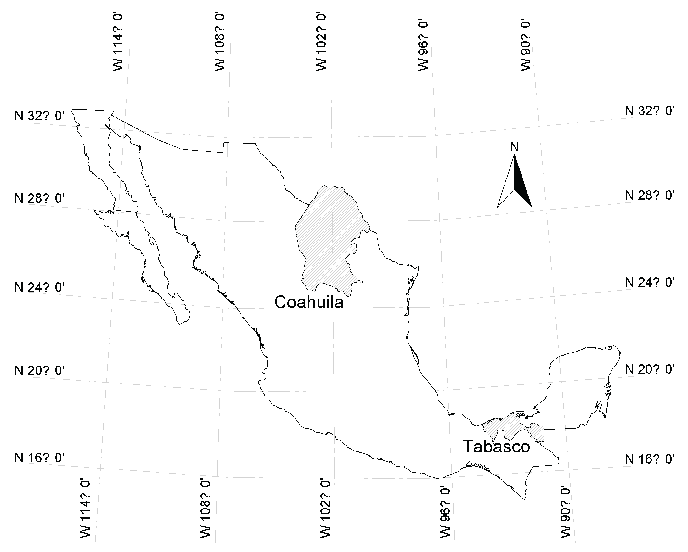
Figure 2.
First stage for delineation of homogeneous regions.
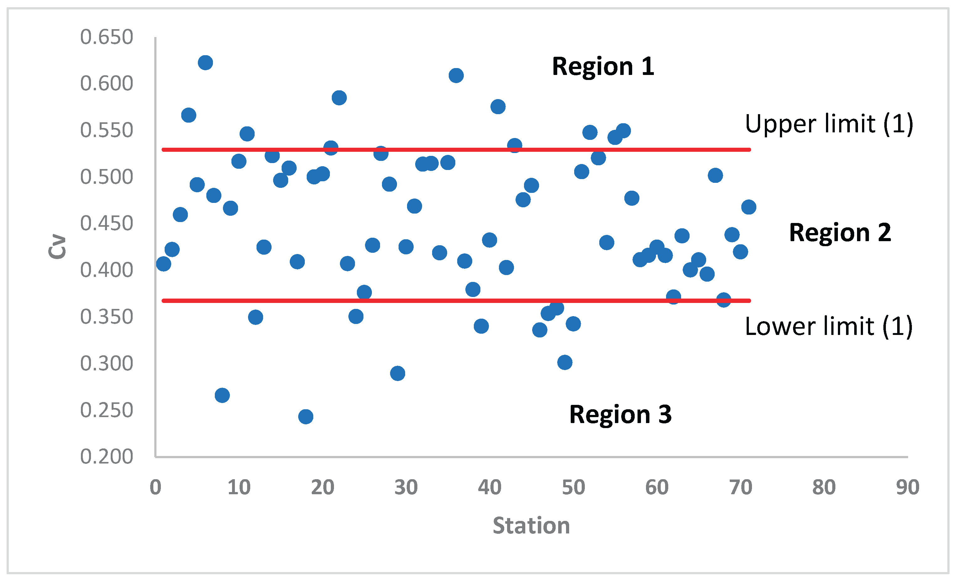
Figure 3.
Second stage for delineation of homogeneous regions.
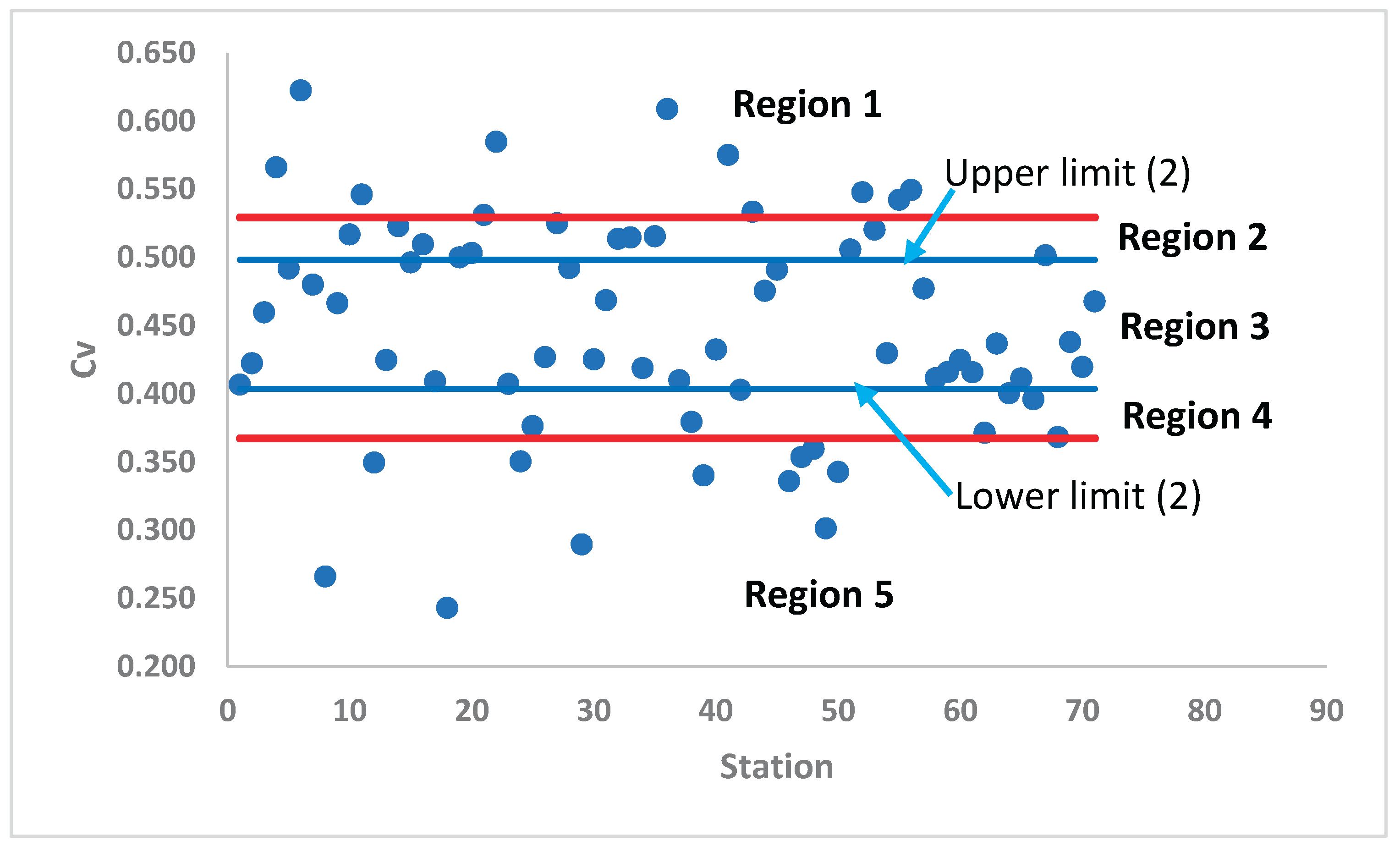
Figure 4.
Final stage for delineation of homogeneous regions.
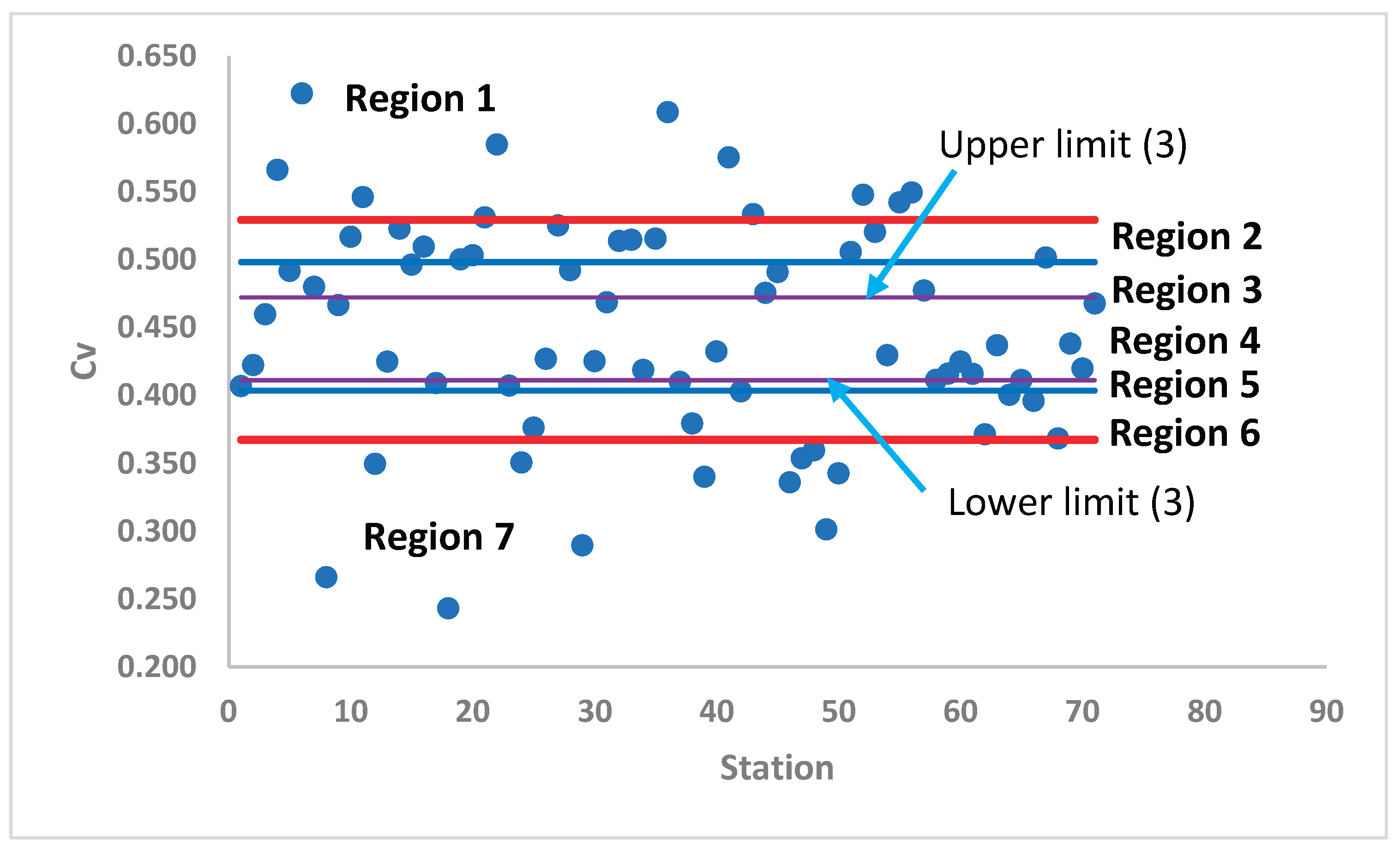

Table 1.
List of 106 rain gauge stations in Coahuila and their corresponding characteristics.
| No | (1) | (2) | (3) | (4) | (5) | (6) | (7) | No | (1) | (2) | (3) | (4) | (5) | (6) | (7) |
|---|---|---|---|---|---|---|---|---|---|---|---|---|---|---|---|
| 1 | 5001 | 100.58 | 27.93 | 370 | 64 | 1950-2013 | 0.567 | 54 | 5068 | 100.99 | 29.16 | 330 | 27 | 1987-2013 | 0.508 |
| 2 | 5002 | 100.83 | 28.33 | 374 | 61 | 1950-2010 | 0.472 | 55 | 5069 | 101.51 | 27.87 | 490 | 34 | 1980-2013 | 0.402 |
| 3 | 5003 | 100.85 | 25.45 | 1660 | 20 | 1956-1975 | 0.685 | 56 | 5074 | 100.92 | 28.49 | 360 | 23 | 1979-2001 | 0.571 |
| 4 | 5004 | 102.63 | 25.12 | 1300 | 50 | 1967-2016 | 0.475 | 57 | 5075 | 100.85 | 28.35 | 380 | 23 | 1979-2001 | 0.570 |
| 5 | 5005 | 100.76 | 26.84 | 582 | 45 | 1967-2011 | 0.662 | 58 | 5081 | 101.11 | 25.12 | 2100 | 45 | 1969-2013 | 0.407 |
| 6 | 5006 | 100.76 | 26.84 | 582 | 41 | 1970-2010 | 0.466 | 59 | 5085 | 101.11 | 25.12 | 2100 | 27 | 1987-2013 | 0.553 |
| 7 | 5007 | 103.12 | 25.78 | 1105 | 67 | 1950-2016 | 0.428 | 60 | 5086 | 100.96 | 29.04 | 340 | 27 | 1987-2013 | 0.685 |
| 8 | 5008 | 101.38 | 27.96 | 380 | 34 | 1980-2013 | 0.331 | 61 | 5130 | 101.32 | 25.85 | 1100 | 45 | 1969-2013 | 0.526 |
| 9 | 5009 | 102.07 | 26.97 | 730 | 33 | 1981-2013 | 0.459 | 62 | 5133 | 103.25 | 25.33 | 1211 | 47 | 1970-2016 | 0.614 |
| 10 | 5011 | 101.08 | 26.13 | 936 | 59 | 1955-2013 | 0.559 | 63 | 5135 | 103.29 | 28.09 | 1080 | 24 | 1990-2013 | 1.424 |
| 11 | 5013 | 102.95 | 28.64 | 1060 | 35 | 1979-2013 | 0.641 | 64 | 5136 | 100.86 | 24.96 | 2110 | 34 | 1980-2013 | 0.442 |
| 12 | 5015 | 102.82 | 28.80 | 1040 | 24 | 1990-2013 | 0.516 | 65 | 5139 | 102.94 | 25.49 | 1110 | 67 | 1950-2016 | 1.054 |
| 13 | 5016 | 101.48 | 25.38 | 1400 | 45 | 1969-2013 | 0.418 | 66 | 5140 | 100.95 | 25.54 | 1400 | 32 | 1980-2011 | 0.773 |
| 14 | 5018 | 102.01 | 25.73 | 1140 | 56 | 1961-2016 | 0.427 | 67 | 5141 | 101.03 | 24.96 | 1920 | 60 | 1954-2013 | 0.508 |
| 15 | 5019 | 101.42 | 26.91 | 615 | 24 | 1987-2010 | 0.567 | 68 | 5142 | 101.40 | 25.70 | 1150 | 45 | 1969-2013 | 0.654 |
| 16 | 5020 | 101.52 | 27.87 | 490 | 35 | 1979-2013 | 0.580 | 69 | 5144 | 102.27 | 26.61 | 800 | 33 | 1981-2013 | 0.451 |
| 17 | 5021 | 101.25 | 27.92 | 369 | 34 | 1980-2013 | 0.290 | 70 | 5145 | 101.22 | 25.25 | 1840 | 45 | 1969-2013 | 0.534 |
| 18 | 5022 | 102.40 | 27.31 | 1100 | 42 | 1960-2001 | 0.552 | 71 | 5146 | 100.83 | 25.21 | 2100 | 60 | 1954-2013 | 0.699 |
| 19 | 5023 | 100.99 | 29.16 | 340 | 27 | 1987-2013 | 0.543 | 72 | 5147 | 101.23 | 27.23 | 463 | 34 | 1980-2013 | 0.694 |
| 20 | 5024 | 102.17 | 25.44 | 1500 | 56 | 1961-2016 | 0.474 | 73 | 5148 | 100.34 | 25.28 | 1740 | 60 | 1954-2013 | 0.904 |
| 21 | 5025 | 100.52 | 28.70 | 250 | 32 | 1979-2010 | 0.390 | 74 | 5149 | 100.53 | 25.34 | 2420 | 60 | 1954-2013 | 0.825 |
| 22 | 5026 | 103.47 | 25.54 | 1223 | 42 | 1969-2010 | 0.448 | 75 | 5150 | 101.43 | 27.18 | 430 | 33 | 1981-2013 | 0.452 |
| 23 | 5027 | 103.34 | 25.70 | 1120 | 61 | 1950-2010 | 0.557 | 76 | 5151 | 101.25 | 25.98 | 920 | 59 | 1955-2013 | 0.500 |
| 24 | 5028 | 103.05 | 25.76 | 1110 | 67 | 1950-2016 | 0.428 | 77 | 5152 | 101.26 | 26.53 | 820 | 33 | 1981-2013 | 0.426 |
| 25 | 5029 | 103.28 | 25.07 | 1300 | 50 | 1967-2016 | 0.773 | 78 | 5153 | 101.42 | 26.77 | 743 | 24 | 1987-2010 | 0.565 |
| 26 | 5030 | 100.62 | 27.52 | 272 | 64 | 1950-2013 | 0.421 | 79 | 5155 | 101.79 | 27.05 | 640 | 33 | 1981-2013 | 0.510 |
| 27 | 5031 | 101.00 | 27.42 | 360 | 64 | 1950-2013 | 0.472 | 80 | 5156 | 101.40 | 27.89 | 430 | 34 | 1980-2013 | 0.386 |
| 28 | 5032 | 100.98 | 25.53 | 1470 | 62 | 1950-2011 | 0.588 | 81 | 5157 | 102.73 | 26.83 | 900 | 36 | 1981-2016 | 0.457 |
| 29 | 5033 | 101.12 | 27.85 | 339 | 64 | 1950-2013 | 0.446 | 82 | 5158 | 101.31 | 26.62 | 920 | 33 | 1981-2013 | 0.414 |
| 30 | 5034 | 101.12 | 27.85 | 339 | 67 | 1950-2016 | 0.474 | 83 | 5159 | 103.04 | 26.48 | 1100 | 61 | 1950-2010 | 0.455 |
| 31 | 5035 | 100.58 | 25.27 | 2180 | 45 | 1954-1998 | 0.539 | 84 | 5160 | 100.85 | 25.45 | 1660 | 18 | 1988-2005 | 1.008 |
| 32 | 5036 | 103.00 | 25.76 | 1100 | 67 | 1950-2016 | 0.493 | 85 | 5162 | 101.58 | 25.36 | 1550 | 45 | 1969-2013 | 0.495 |
| 33 | 5037 | 102.22 | 25.62 | 1170 | 60 | 1957-2016 | 0.462 | 86 | 5163 | 101.73 | 27.23 | 640 | 34 | 1980-2013 | 0.487 |
| 34 | 5038 | 101.35 | 26.39 | 1010 | 33 | 1981-2013 | 0.653 | 87 | 5164 | 101.65 | 27.14 | 500 | 33 | 1981-2013 | 0.389 |
| 35 | 5039 | 103.70 | 27.29 | 1256 | 54 | 1960-2013 | 0.557 | 88 | 5166 | 101.35 | 27.75 | 450 | 34 | 1980-2013 | 0.403 |
| 36 | 5040 | 103.43 | 25.52 | 1123 | 41 | 1970-2010 | 0.572 | 89 | 5167 | 101.36 | 26.64 | 660 | 33 | 1981-2013 | 0.371 |
| 37 | 5041 | 102.81 | 25.32 | 1100 | 45 | 1972-2016 | 0.477 | 90 | 5168 | 103.42 | 28.38 | 1180 | 24 | 1990-2013 | 0.654 |
| 38 | 5042 | 100.93 | 28.49 | 360 | 24 | 1954-1977 | 0.747 | 91 | 5169 | 101.37 | 27.20 | 850 | 33 | 1981-2013 | 0.414 |
| 39 | 5043 | 100.85 | 28.34 | 380 | 23 | 1979-2001 | 0.585 | 92 | 5170 | 101.39 | 25.52 | 1680 | 45 | 1969-2013 | 1.137 |
| 40 | 5044 | 102.07 | 26.99 | 740 | 64 | 1950-2013 | 0.482 | 93 | 5171 | 101.72 | 27.00 | 1275 | 33 | 1981-2013 | 0.782 |
| 41 | 5045 | 100.73 | 27.61 | 280 | 64 | 1950-2013 | 0.600 | 94 | 5174 | 100.88 | 25.45 | 1670 | 31 | 1981-2011 | 0.483 |
| 42 | 5046 | 103.66 | 27.29 | 1383 | 13 | 1953-1965 | 0.870 | 95 | 5175 | 100.89 | 24.64 | 1867 | 41 | 1973-2013 | 0.488 |
| 43 | 5047 | 101.42 | 26.90 | 586 | 35 | 1951-1985 | 0.509 | 96 | 5176 | 100.62 | 25.37 | 2759 | 60 | 1954-2013 | 0.437 |
| 44 | 5048 | 101.00 | 25.43 | 1700 | 64 | 1950-2013 | 0.579 | 97 | 5178 | 103.21 | 25.28 | 1200 | 47 | 1970-2016 | 0.526 |
| 45 | 5049 | 100.62 | 25.28 | 2300 | 26 | 1988-2013 | 0.434 | 98 | 5179 | 102.21 | 26.93 | 1091 | 36 | 1981-2016 | 0.550 |
| 46 | 5050 | 101.53 | 27.05 | 510 | 33 | 1981-2013 | 0.344 | 99 | 5180 | 103.26 | 25.77 | 1116 | 67 | 1950-2016 | 0.375 |
| 47 | 5051 | 102.80 | 25.35 | 1093 | 67 | 1950-2016 | 0.544 | 100 | 5181 | 102.62 | 25.62 | 1109 | 18 | 1991-2008 | 0.597 |
| 48 | 5052 | 102.80 | 25.35 | 1093 | 24 | 1987-2010 | 0.528 | 101 | 5182 | 102.22 | 26.94 | 836 | 33 | 1981-2013 | 0.376 |
| 49 | 5058 | 103.30 | 28.45 | 1080 | 24 | 1990-2013 | 0.445 | 102 | 5184 | 102.95 | 24.81 | 1460 | 50 | 1967-2016 | 0.328 |
| 50 | 5060 | 101.25 | 25.27 | 1880 | 45 | 1969-2013 | 0.639 | 103 | 5185 | 102.95 | 24.81 | 1460 | 67 | 1950-2016 | 0.327 |
| 51 | 5063 | 100.86 | 28.35 | 380 | 23 | 1979-2001 | 0.542 | 104 | 5186 | 101.08 | 29.04 | 348 | 27 | 1987-2013 | 0.474 |
| 52 | 5065 | 100.76 | 26.84 | 420 | 61 | 1951-2011 | 0.546 | 105 | 5188 | 101.11 | 26.85 | 958 | 33 | 1981-2013 | 0.496 |
| 53 | 5066 | 101.12 | 27.84 | 339 | 34 | 1980-2013 | 0.332 | 106 | 5189 | 100.77 | 27.59 | 285 | 64 | 1950-2013 | 0.527 |
(1) Station code, (2) Longitude (W), (3) Latitude (N), (4) Altitude (masl), (5) Record length (yr.), (6) Period of data, and (7) Coefficient of variation of annual maximum daily rainfall series (Cv).
Table 2.
List of 75 rain gauge stations in Tabasco and their corresponding characteristics.
| No | 1 | 2 | 3 | 4 | 5 | 6 | 7 | No | 1 | 2 | 3 | 4 | 5 | 6 | 7 |
|---|---|---|---|---|---|---|---|---|---|---|---|---|---|---|---|
| 1 | 27001 | 17.81 | 91.54 | 18.00 | 32 | 1950-1981 | 0.355 | 39 | 27042 | 17.46 | 92.78 | 44.00 | 58 | 1960-2017 | 0.347 |
| 2 | 27002 | 18.42 | 92.80 | 3.00 | 68 | 1950-2017 | 0.495 | 40 | 27044 | 17.55 | 92.95 | 51.00 | 58 | 1960-2017 | 0.270 |
| 3 | 27003 | 18.05 | 93.97 | 5.00 | 56 | 1961-2016 | 0.538 | 41 | 27045 | 17.57 | 92.97 | 54.00 | 56 | 1962-2017 | 0.283 |
| 4 | 27004 | 17.45 | 91.49 | 14.00 | 67 | 1950-2016 | 0.312 | 42 | 27046 | 17.47 | 91.43 | 19.00 | 63 | 1954-2016 | 0.323 |
| 5 | 27006 | 17.64 | 91.27 | 50.00 | 63 | 1954-2016 | 0.415 | 43 | 27047 | 17.47 | 91.43 | 22.00 | 63 | 1954-2016 | 0.332 |
| 6 | 27007 | 18.00 | 93.62 | 12.00 | 57 | 1961-2017 | 0.378 | 44 | 27048 | 17.82 | 92.37 | 7.00 | 68 | 1950-2017 | 0.373 |
| 7 | 27008 | 18.00 | 93.38 | 25.00 | 63 | 1955-2017 | 0.416 | 45 | 27049 | 17.72 | 92.81 | 13.00 | 67 | 1951-2017 | 0.418 |
| 8 | 27009 | 18.25 | 93.22 | 15.00 | 68 | 1950-2017 | 0.415 | 46 | 27050 | 18.38 | 92.60 | 2.00 | 68 | 1950-2017 | 0.394 |
| 9 | 27010 | 18.07 | 93.18 | 15.00 | 63 | 1955-2017 | 0.375 | 47 | 27051 | 18.11 | 93.35 | 20.00 | 68 | 1950-2017 | 0.353 |
| 10 | 27011 | 17.61 | 92.80 | 20.00 | 67 | 1951-2017 | 0.521 | 48 | 27053 | 18.39 | 92.88 | 6.00 | 68 | 1950-2017 | 0.381 |
| 11 | 27012 | 17.74 | 91.76 | 26.00 | 23 | 1995-2016 | 0.254 | 49 | 27054 | 18.00 | 92.93 | 24.00 | 27 | 1972-1998 | 0.449 |
| 12 | 27013 | 18.25 | 93.55 | 11.00 | 15 | 1965-1979 | 0.341 | 50 | 27055 | 17.98 | 92.92 | 6.00 | 48 | 1950-1997 | 0.407 |
| 13 | 27014 | 18.02 | 92.93 | 7.00 | 13 | 1968-1980 | 0.567 | 51 | 27056 | 17.81 | 91.54 | 12.00 | 31 | 1986-2016 | 0.402 |
| 14 | 27015 | 17.84 | 93.94 | 7.00 | 64 | 1954-2017 | 0.312 | 52 | 27057 | 18.27 | 93.22 | 13.00 | 68 | 1950-2017 | 0.569 |
| 15 | 27016 | 18.53 | 92.63 | 2.00 | 68 | 1950-2017 | 0.409 | 53 | 27059 | 17.94 | 91.18 | 41.00 | 64 | 1954-2017 | 0.407 |
| 16 | 27017 | 17.83 | 93.39 | 36.00 | 68 | 1950-2017 | 0.337 | 54 | 27060 | 17.97 | 93.77 | 11.00 | 57 | 1961-2017 | 0.352 |
| 17 | 27018 | 17.87 | 93.47 | 29.00 | 68 | 1950-2017 | 0.335 | 55 | 27061 | 17.51 | 92.92 | 86.00 | 56 | 1962-2017 | 0.345 |
| 18 | 27019 | 17.72 | 92.81 | 14.00 | 67 | 1951-2017 | 0.303 | 56 | 27065 | 17.99 | 92.83 | 14.00 | 48 | 1950-1997 | 0.400 |
| 19 | 27020 | 18.17 | 93.05 | 10.00 | 68 | 1950-2017 | 0.500 | 57 | 27068 | 17.53 | 92.93 | 78.00 | 56 | 1962-2017 | 0.314 |
| 20 | 27021 | 17.76 | 91.29 | 29.00 | 63 | 1954-2016 | 0.356 | 58 | 27069 | 17.86 | 91.78 | 5.00 | 31 | 1986-2016 | 0.242 |
| 21 | 27022 | 17.63 | 92.54 | 24.00 | 50 | 1950-1999 | 0.350 | 59 | 27070 | 17.38 | 92.75 | 63.00 | 58 | 1960-2017 | 0.329 |
| 22 | 27024 | 17.52 | 92.93 | 80.00 | 56 | 1962-2017 | 0.364 | 60 | 27071 | 17.80 | 92.48 | 11.00 | 67 | 1950-2016 | 0.361 |
| 23 | 27026 | 18.10 | 94.05 | 10.00 | 63 | 1954-2016 | 0.484 | 61 | 27073 | 18.17 | 93.49 | 7.00 | 46 | 1972-2017 | 0.449 |
| 24 | 27027 | 17.59 | 92.70 | 22.00 | 67 | 1951-2017 | 0.370 | 62 | 27075 | 18.11 | 93.57 | 10.00 | 46 | 1972-2017 | 0.434 |
| 25 | 27028 | 18.09 | 92.14 | 6.00 | 68 | 1950-2017 | 0.398 | 63 | 27076 | 18.11 | 93.50 | 13.00 | 46 | 1972-2017 | 0.548 |
| 26 | 27029 | 18.14 | 92.86 | 10.00 | 68 | 1950-2017 | 0.369 | 64 | 27077 | 18.07 | 93.62 | 12.00 | 46 | 1972-2017 | 0.392 |
| 27 | 27030 | 17.76 | 92.61 | 11.00 | 67 | 1950-2016 | 0.283 | 65 | 27078 | 18.02 | 93.50 | 19.00 | 46 | 1972-2017 | 0.439 |
| 28 | 27031 | 17.75 | 92.60 | 10.00 | 67 | 1950-2016 | 0.436 | 66 | 27079 | 18.05 | 93.44 | 21.00 | 11 | 1969-1979 | 0.369 |
| 29 | 27032 | 17.65 | 93.40 | 44.00 | 68 | 1950-2017 | 0.319 | 67 | 27080 | 17.97 | 93.50 | 21.00 | 57 | 1961-2017 | 0.370 |
| 30 | 27033 | 17.73 | 93.63 | 50.00 | 68 | 1950-2017 | 0.329 | 68 | 27083 | 17.98 | 92.93 | 27.00 | 12 | 2005-2016 | 0.468 |
| 31 | 27034 | 18.40 | 93.21 | 6.00 | 68 | 1950-2017 | 0.369 | 69 | 27084 | 18.17 | 93.02 | 10.00 | 68 | 1950-2017 | 0.457 |
| 32 | 27035 | 17.76 | 93.38 | 36.00 | 68 | 1950-2017 | 0.303 | 70 | 27087 | 17.99 | 91.39 | 54.00 | 31 | 1986-2016 | 0.320 |
| 33 | 27036 | 18.07 | 93.18 | 15.00 | 68 | 1950-2017 | 0.439 | 71 | 27088 | 17.62 | 91.55 | 67.00 | 17 | 1983-1999 | 0.432 |
| 34 | 27037 | 17.85 | 93.88 | 21.00 | 68 | 1950-2017 | 0.385 | 72 | 27090 | 17.97 | 91.60 | 10.00 | 31 | 1986-2016 | 0.331 |
| 35 | 27038 | 18.30 | 93.07 | 7.00 | 68 | 1950-2017 | 0.524 | 73 | 27091 | 17.94 | 91.81 | 5.00 | 31 | 1986-2016 | 0.303 |
| 36 | 27039 | 18.00 | 93.28 | 23.00 | 68 | 1950-2017 | 0.375 | 74 | 27092 | 17.85 | 92.93 | 18.00 | 18 | 2000-2017 | 0.313 |
| 37 | 27040 | 17.79 | 91.16 | 44.00 | 65 | 1952-2016 | 0.403 | 75 | 27093 | 18.01 | 91.56 | 14.00 | 31 | 1986-2016 | 0.295 |
| 38 | 27041 | 18.09 | 93.35 | 20.00 | 63 | 1955-2017 | 0.337 |
(1) Station code, (2) Longitude (W), (3) Latitude (N), (4) Altitude (masl), (5) Record length (yr.), (6) Period of data, and (7) Coefficient of variation of annual maximum daily rainfall series (Cv).
Table 3.
Quantile biases obtained for the EG marginal with length .
| Sample Sizes | Non exceedance probability | ||||||
|---|---|---|---|---|---|---|---|
| n1 | n2 | 0.50 | 0.80 | 0.90 | 0.95 | 0.98 | 0.99 |
| 10 | 10 | -0.0394 | 0.1823 | 0.3623 | 0.5524 | 0.8167 | 1.0247 |
| 10 | 20 | -0.0944 | 0.0571 | 0.1929 | 0.3415 | 0.5531 | 0.7220 |
| 20 | 20 | -0.0849 | 0.0387 | 0.1474 | 0.2657 | 0.4336 | 0.5673 |
| 20 | 50 | -0.1037 | -0.0427 | 0.0300 | 0.1167 | 0.2466 | 0.3533 |
| 50 | 50 | -0.0764 | -0.0112 | 0.0596 | 0.1418 | 0.2630 | 0.3617 |
| 50 | 100 | -0.0618 | -0.0554 | 0.0470 | 0.0612 | 0.1644 | 0.2510 |
Table 4.
Quantile MSE’s obtained for the EG marginal with length .
| Sample Sizes | Non exceedance probability | ||||||
|---|---|---|---|---|---|---|---|
| n1 | n2 | 0.50 | 0.80 | 0.90 | 0.95 | 0.98 | 0.99 |
| 10 | 10 | 0.9016 | 2.1029 | 3.3334 | 4.8397 | 7.2743 | 9.4667 |
| 10 | 20 | 0.8650 | 1.8796 | 3.0143 | 4.4338 | 6.7517 | 8.8482 |
| 20 | 20 | 0.4006 | 0.8913 | 1.4458 | 2.1516 | 3.3257 | 4.4039 |
| 20 | 50 | 0.3771 | 0.8721 | 1.4153 | 2.0979 | 3.2235 | 4.2517 |
| 50 | 50 | 0.1683 | 0.3966 | 0.6547 | 0.9854 | 1.5414 | 2.0573 |
| 50 | 100 | 0.1659 | 0.3916 | 0.6339 | 0.9398 | 1.4491 | 1.9196 |
Table 5.
Stations by homogeneous region “R” in Coahuila.
| R1 | R2 | R3 | R4 | R5 | R6 | R7 | R8 | R9 |
|---|---|---|---|---|---|---|---|---|
| 5029 | 5003 | 5001 | 5022 | 5015 | 5002 | 5009 | 5007 | 5008 |
| 5042 | 5005 | 5011 | 5023 | 5036 | 5004 | 5026 | 5016 | 5021 |
| 5046 | 5013 | 5019 | 5035 | 5044 | 5006 | 5033 | 5018 | 5050 |
| 5135 | 5038 | 5020 | 5051 | 5047 | 5024 | 5037 | 5025 | 5066 |
| 5139 | 5045 | 5027 | 5063 | 5052 | 5031 | 5049 | 5028 | 5167 |
| 5140 | 5060 | 5032 | 5065 | 5068 | 5034 | 5058 | 5030 | 5184 |
| 5148 | 5086 | 5039 | 5085 | 5130 | 5041 | 5136 | 5069 | 5185 |
| 5149 | 5133 | 5040 | 5179 | 5141 | 5186 | 5144 | 5081 | |
| 5160 | 5142 | 5043 | 5145 | 5150 | 5152 | |||
| 5170 | 5146 | 5048 | 5151 | 5157 | 5156 | |||
| 5171 | 5147 | 5074 | 5155 | 5159 | 5158 | |||
| 5168 | 5075 | 5162 | 5176 | 5164 | ||||
| 5181 | 5153 | 5163 | 5166 | |||||
| 5174 | 5169 | |||||||
| 5175 | 5180 | |||||||
| 5178 | 5182 | |||||||
| 5188 | ||||||||
| 5189 |
Table 6.
Stations by homogeneous region “R” in Tabasco.
| R1 | R2 | R3 | R4 | R5 | R6 | R7 |
| 27002 | 27006 | 27016 | 27001 | 27013 | 27004 | 27012 |
| 27003 | 27008 | 27028 | 27007 | 27017 | 27015 | 27019 |
| 27011 | 27009 | 27040 | 27010 | 27018 | 27032 | 27030 |
| 27014 | 27031 | 27050 | 27021 | 27041 | 27033 | 27035 |
| 27020 | 27036 | 27055 | 27022 | 27042 | 27046 | 27044 |
| 27026 | 27049 | 27056 | 27024 | 27061 | 27047 | 27045 |
| 27038 | 27054 | 27059 | 27027 | 27068 | 27069 | |
| 27057 | 27073 | 27065 | 27029 | 27070 | 27091 | |
| 27076 | 27075 | 27034 | 27087 | 27093 | ||
| 27083 | 27078 | 27037 | 27090 | |||
| 27084 | 27088 | 27039 | 27092 | |||
| 27048 | ||||||
| 27051 | ||||||
| 27053 | ||||||
| 27060 | ||||||
| 27071 | ||||||
| 27077 | ||||||
| 27079 | ||||||
| 27080 |
Table 7.
Examples of BEG model combinations applied to selected stations in Coahuila.
| Station | Neighboring | Relative sample sizes | Bivariate parameters | Marginal (1) | ||||||||||
|---|---|---|---|---|---|---|---|---|---|---|---|---|---|---|
| Region | base | station | n1 | n2 | n3 | Loc 1 | Sca 1 | Shp 1 | Loc 2 | Sca 2 | Shp 2 | m | AICc | BIC |
| 3 | 5020 | 5032 | 29 | 33 | 2 | 67.54 | 37.27 | 1.22 | 31.88 | 12.98 | 0.83 | 1.15 | 342.0 | 345.9 |
| 5040 | 9 | 32 | 3 | 64.77 | 37.85 | 1.11 | 35.08 | 18.13 | 0.83 | 1.14 | 347.5 | 351.4 | ||
| 5153 | 8 | 24 | 3 | 57.38 | 36.47 | 0.93 | 39.76 | 23.10 | 0.96 | 1.04 | 353.4 | 357.3 | ||
| 5019 | 8 | 24 | 3 | 55.72 | 32.19 | 0.81 | 32.52 | 16.02 | 0.92 | 1.09 | 356.7 | 360.6 | ||
| 5001 | 29 | 35 | 0 | 64.38 | 37.87 | 1.07 | 51.19 | 30.33 | 1.00 | 1.04 | 358.3 | 362.1 | ||
| 5074 | 0 | 23 | 12 | 59.85 | 36.82 | 0.94 | 70.66 | 29.77 | 0.92 | 1.20 | 360.9 | 364.7 | ||
| 5075 | 0 | 23 | 12 | 63.11 | 37.02 | 1.01 | 71.22 | 37.63 | 0.84 | 1.21 | 371.8 | 375.7 | ||
| 5043 | 0 | 23 | 12 | 64.17 | 37.22 | 1.03 | 69.69 | 36.79 | 0.81 | 1.21 | 373.6 | 377.5 | ||
| 5 | 5163 | 5044 | 30 | 34 | 0 | 52.47 | 26.04 | 1.08 | 28.28 | 10.82 | 0.54 | 1.12 | 307.7 | 311.5 |
| 5145 | 11 | 34 | 0 | 42.86 | 21.58 | 0.70 | 37.11 | 12.00 | 0.83 | 1.29 | 311.6 | 315.4 | ||
| 5178 | 10 | 34 | 3 | 45.83 | 21.41 | 0.69 | 37.77 | 14.68 | 0.89 | 1.37 | 313.8 | 317.5 | ||
| 5162 | 11 | 34 | 0 | 50.50 | 24.56 | 0.97 | 35.09 | 14.31 | 0.72 | 1.02 | 314.6 | 318.4 | ||
| 5141 | 26 | 34 | 0 | 49.01 | 24.53 | 0.98 | 38.17 | 13.42 | 0.80 | 1.05 | 314.7 | 318.4 | ||
| 5052 | 7 | 24 | 3 | 47.41 | 21.63 | 0.88 | 35.32 | 17.94 | 0.86 | 1.14 | 323.2 | 327.0 | ||
| 5174 | 1 | 31 | 2 | 52.21 | 23.84 | 1.09 | 31.13 | 11.25 | 0.73 | 1.16 | 324.3 | 328.1 | ||
| 5188 | 1 | 33 | 0 | 44.00 | 19.64 | 0.70 | 46.18 | 22.24 | 1.12 | 1.07 | 327.1 | 330.9 | ||
| 5155 | 1 | 33 | 0 | 50.34 | 24.18 | 1.00 | 43.41 | 23.08 | 0.98 | 1.37 | 327.7 | 331.5 | ||
| 5047 | 29 | 6 | 28 | 49.54 | 23.72 | 1.00 | 47.53 | 22.96 | 0.90 | 2.31 | 332.0 | 335.7 | ||
| 5189 | 30 | 34 | 0 | 50.33 | 24.55 | 1.00 | 59.26 | 24.58 | 0.87 | 1.16 | 380.6 | 384.4 | ||
| 5068 | 7 | 27 | 0 | 51.23 | 24.55 | 1.00 | 79.24 | 35.89 | 0.83 | 1.03 | 391.8 | 395.6 | ||
| 7 | 5009 | 5136 | 1 | 33 | 0 | 31.74 | 15.29 | 0.89 | 33.32 | 11.26 | 0.85 | 1.10 | 282.7 | 286.4 |
| 5144 | 0 | 33 | 0 | 32.04 | 15.94 | 0.91 | 28.97 | 14.07 | 0.82 | 1.50 | 290.3 | 294.0 | ||
| 5159 | 31 | 30 | 3 | 31.51 | 15.30 | 0.84 | 29.56 | 14.07 | 0.91 | 1.05 | 295.3 | 299.0 | ||
| 5176 | 27 | 33 | 0 | 36.07 | 16.46 | 1.09 | 28.56 | 9.34 | 0.59 | 1.08 | 296.9 | 300.5 | ||
| 5150 | 0 | 33 | 0 | 31.53 | 15.29 | 0.88 | 33.95 | 16.04 | 0.87 | 1.34 | 297.6 | 301.3 | ||
| 5037 | 24 | 33 | 3 | 40.51 | 21.42 | 1.65 | 26.68 | 9.73 | 0.54 | 1.06 | 302.1 | 305.8 | ||
| 5049 | 7 | 26 | 0 | 33.41 | 16.48 | 1.04 | 40.12 | 15.08 | 0.81 | 1.08 | 308.0 | 311.7 | ||
| 5033 | 31 | 33 | 0 | 31.54 | 15.67 | 0.96 | 60.91 | 27.60 | 0.93 | 1.17 | 495.1 | 498.7 | ||
| 8 | 5018 | 5158 | 20 | 33 | 3 | 26.77 | 12.18 | 0.80 | 27.47 | 11.31 | 0.98 | 1.29 | 453.3 | 458.9 |
| 5182 | 20 | 33 | 3 | 27.72 | 12.21 | 0.87 | 28.99 | 11.06 | 0.91 | 1.17 | 456.1 | 461.7 | ||
| 5016 | 8 | 45 | 3 | 28.37 | 12.21 | 0.92 | 33.40 | 14.35 | 0.86 | 1.19 | 493.7 | 499.3 | ||
| 5081 | 8 | 45 | 3 | 28.21 | 12.21 | 0.94 | 34.29 | 11.25 | 0.71 | 1.06 | 498.0 | 503.6 | ||
| 5152 | 20 | 33 | 3 | 26.92 | 12.22 | 0.81 | 42.30 | 18.92 | 0.89 | 1.05 | 514.9 | 520.5 | ||
| 5164 | 20 | 33 | 3 | 28.36 | 12.20 | 0.91 | 46.12 | 13.97 | 0.87 | 1.18 | 516.2 | 521.8 | ||
| 5166 | 19 | 34 | 3 | 28.07 | 12.21 | 0.91 | 58.84 | 26.49 | 1.08 | 1.15 | 601.4 | 607.0 | ||
| 5156 | 19 | 34 | 3 | 26.96 | 12.22 | 0.83 | 64.71 | 24.54 | 1.03 | 1.11 | 607.6 | 613.2 | ||
| 5069 | 19 | 34 | 3 | 27.29 | 12.22 | 0.82 | 64.32 | 26.19 | 0.92 | 1.08 | 625.7 | 631.3 | ||
| 5025 | 18 | 32 | 6 | 28.18 | 12.22 | 0.88 | 75.66 | 28.81 | 1.01 | 1.18 | 674.3 | 679.9 | ||
| 5030 | 11 | 53 | 3 | 27.96 | 12.22 | 0.88 | 59.95 | 24.26 | 0.96 | 1.54 | 726.5 | 732.1 | ||
Loc = location parameter; Sca = Scale parameter; Shp = Shape parameter; Marginal (1) = Station base.
Table 8.
Examples of return levels (mm) estimated with the BEG distribution for selected base stations in Coahuila.
Table 8.
Examples of return levels (mm) estimated with the BEG distribution for selected base stations in Coahuila.
| Station | Neighboring | Return period T(years) | |||||||||||
|---|---|---|---|---|---|---|---|---|---|---|---|---|---|
| Region | base | Station | 1.1 | 2 | 5 | 10 | 20 | 50 | 100 | 500 | 1000 | 5000 | 10000 |
| 3 | 5020 | 5032 | 32.0 | 74.1 | 110.9 | 134.6 | 157.1 | 185.8 | 207.3 | 256.6 | 277.8 | 326.8 | 347.9 |
| 5040 | 30.2 | 74.9 | 114.9 | 141.1 | 166.0 | 198.1 | 222.1 | 277.4 | 301.1 | 356.2 | 379.9 | ||
| 5153 | 26.5 | 73.3 | 116.7 | 145.7 | 173.7 | 209.9 | 237.2 | 300.1 | 327.2 | 390.1 | 417.2 | ||
| 5019 | 30.5 | 75.0 | 117.8 | 146.8 | 175.1 | 212.0 | 239.8 | 304.2 | 331.9 | 396.2 | 423.9 | ||
| 5001 | 30.3 | 75.9 | 116.9 | 143.9 | 169.6 | 202.8 | 227.7 | 285.1 | 309.7 | 366.9 | 391.5 | ||
| 5074 | 28.5 | 75.6 | 119.1 | 148.2 | 176.2 | 212.5 | 239.7 | 302.7 | 329.8 | 392.7 | 419.8 | ||
| 5075 | 30.5 | 76.2 | 117.8 | 145.3 | 171.6 | 205.7 | 231.2 | 290.2 | 315.5 | 374.4 | 399.7 | ||
| 5043 | 31.2 | 76.7 | 118.0 | 145.2 | 171.3 | 204.9 | 230.2 | 288.4 | 313.5 | 371.6 | 396.6 | ||
| 5 | 5163 | 5044 | 28.9 | 60.0 | 88.0 | 106.3 | 123.8 | 146.3 | 163.2 | 202.1 | 218.8 | 257.6 | 274.3 |
| 5145 | 27.2 | 59.4 | 91.3 | 113.3 | 134.9 | 163.2 | 184.6 | 234.1 | 255.5 | 305.0 | 326.3 | ||
| 5178 | 30.4 | 62.5 | 94.3 | 116.4 | 138.0 | 166.4 | 187.8 | 237.4 | 258.8 | 308.4 | 329.8 | ||
| 5162 | 29.3 | 60.1 | 88.5 | 107.3 | 125.4 | 148.8 | 166.4 | 207.0 | 224.5 | 265.0 | 282.5 | ||
| 5141 | 27.7 | 58.4 | 86.5 | 105.1 | 123.0 | 146.2 | 163.6 | 203.8 | 221.1 | 261.2 | 278.5 | ||
| 5052 | 29.6 | 58.3 | 85.2 | 103.4 | 120.9 | 143.7 | 160.9 | 200.6 | 217.7 | 257.4 | 274.5 | ||
| 5174 | 30.5 | 58.9 | 84.3 | 101.0 | 116.8 | 137.3 | 152.6 | 187.9 | 203.0 | 238.2 | 253.3 | ||
| 5188 | 29.8 | 59.1 | 88.2 | 108.4 | 128.1 | 154.0 | 173.5 | 218.8 | 238.3 | 283.5 | 303.0 | ||
| 5155 | 29.2 | 59.2 | 86.6 | 104.7 | 122.1 | 144.6 | 161.5 | 200.5 | 217.2 | 256.1 | 272.9 | ||
| 5047 | 28.8 | 58.1 | 84.9 | 102.7 | 119.7 | 141.7 | 158.2 | 196.3 | 212.7 | 250.8 | 267.1 | ||
| 5189 | 28.9 | 59.4 | 87.4 | 105.9 | 123.6 | 146.6 | 163.8 | 203.6 | 220.8 | 260.5 | 277.6 | ||
| 5068 | 29.8 | 60.3 | 88.1 | 106.5 | 124.2 | 147.1 | 164.3 | 204.0 | 221.0 | 260.6 | 277.6 | ||
| 7 | 5009 | 5136 | 19.1 | 39.2 | 58.0 | 70.6 | 82.8 | 98.7 | 110.7 | 138.3 | 150.2 | 177.8 | 189.7 |
| 5144 | 18.7 | 39.5 | 58.9 | 71.9 | 84.5 | 100.8 | 113.1 | 141.4 | 153.7 | 182.0 | 194.2 | ||
| 5159 | 19.2 | 39.9 | 59.5 | 72.8 | 85.7 | 102.4 | 115.0 | 144.3 | 156.9 | 186.1 | 198.7 | ||
| 5176 | 21.1 | 40.7 | 58.3 | 69.8 | 80.7 | 94.9 | 105.5 | 129.8 | 140.3 | 164.6 | 175.1 | ||
| 5150 | 19.0 | 39.2 | 58.3 | 71.1 | 83.6 | 99.7 | 111.9 | 140.0 | 152.1 | 180.2 | 192.3 | ||
| 5037 | 17.8 | 39.0 | 56.5 | 67.3 | 77.4 | 90.1 | 99.5 | 120.7 | 129.8 | 150.7 | 159.7 | ||
| 5049 | 18.7 | 38.7 | 56.9 | 68.8 | 80.2 | 95.0 | 106.0 | 131.5 | 142.4 | 167.8 | 178.8 | ||
| 5033 | 18.1 | 37.9 | 56.1 | 68.3 | 79.9 | 95.1 | 106.4 | 132.7 | 143.9 | 170.1 | 181.4 | ||
| 8 | 5018 | 5158 | 17.2 | 34.1 | 50.4 | 61.5 | 72.2 | 86.2 | 96.8 | 121.3 | 131.9 | 156.4 | 166.9 |
| 5182 | 17.7 | 33.9 | 49.2 | 59.5 | 69.4 | 82.3 | 92.1 | 114.6 | 124.3 | 146.8 | 156.5 | ||
| 5016 | 18.1 | 33.9 | 48.5 | 58.4 | 67.8 | 80.1 | 89.3 | 110.7 | 119.9 | 141.2 | 150.4 | ||
| 5081 | 17.8 | 33.4 | 47.8 | 57.5 | 66.7 | 78.7 | 87.8 | 108.6 | 117.6 | 138.4 | 147.4 | ||
| 5152 | 17.3 | 34.2 | 50.4 | 61.5 | 72.2 | 86.2 | 96.7 | 121.1 | 131.6 | 156.0 | 166.5 | ||
| 5164 | 18.1 | 34.0 | 48.7 | 58.6 | 68.1 | 80.5 | 89.8 | 111.3 | 120.5 | 142.0 | 151.3 | ||
| 5166 | 17.8 | 33.7 | 48.4 | 58.3 | 67.8 | 80.2 | 89.5 | 111.0 | 120.3 | 141.8 | 151.0 | ||
| 5156 | 17.2 | 33.8 | 49.6 | 60.3 | 70.7 | 84.3 | 94.5 | 118.1 | 128.3 | 151.9 | 162.1 | ||
| 5069 | 17.6 | 34.3 | 50.3 | 61.2 | 71.7 | 85.4 | 95.8 | 119.8 | 130.1 | 154.0 | 164.3 | ||
| 5025 | 18.1 | 34.3 | 49.5 | 59.7 | 69.6 | 82.4 | 92.1 | 114.5 | 124.1 | 146.5 | 156.1 | ||
| 5030 | 17.9 | 34.1 | 49.3 | 59.6 | 69.5 | 82.4 | 92.1 | 114.6 | 124.3 | 146.7 | 156.4 | ||
Table 9.
Return levels (mm) from alternative univariate distributions (Gumbel, GEV, and Exponentiated Gumbel), ordered by best fit for selected Coahuila stations.
Table 9.
Return levels (mm) from alternative univariate distributions (Gumbel, GEV, and Exponentiated Gumbel), ordered by best fit for selected Coahuila stations.
| Station | Return period T(years) | |||||||||||||
|---|---|---|---|---|---|---|---|---|---|---|---|---|---|---|
| base | Distribution | 1.1 | 2 | 5 | 10 | 20 | 50 | 100 | 500 | 1000 | 5000 | 10000 | AICc | BIC |
| 5020 | BEG | 32.0 | 74.1 | 110.9 | 134.6 | 157.1 | 185.8 | 207.3 | 256.6 | 277.8 | 326.8 | 347.9 | 342.0 | 345.9 |
| EVI | 31.3 | 75.5 | 116.0 | 142.7 | 168.4 | 201.7 | 226.6 | 284.1 | 308.9 | 366.3 | 391.0 | 366.2 | 369.0 | |
| EG | 31.7 | 72.6 | 116.9 | 148.7 | 180.3 | 221.9 | 253.4 | 326.6 | 358.0 | 431.2 | 462.7 | 368.1 | 372.0 | |
| GEV | 31.8 | 73.8 | 115.9 | 145.8 | 176.3 | 218.3 | 251.9 | 336.8 | 376.7 | 478.1 | 525.8 | 368.3 | 372.2 | |
| BEG | 28.9 | 60.0 | 88.0 | 106.3 | 123.8 | 146.3 | 163.2 | 202.1 | 218.8 | 257.6 | 274.3 | 307.7 | 311.5 | |
| 5163 | EVI | 29.2 | 59.2 | 86.5 | 104.6 | 122.0 | 144.5 | 161.3 | 200.3 | 217.0 | 255.9 | 272.6 | 329.2 | 331.9 |
| EG | 29.6 | 57.1 | 87.0 | 108.6 | 129.9 | 158.1 | 179.4 | 228.9 | 250.2 | 299.7 | 321.0 | 331.1 | 334.9 | |
| GEV | 29.5 | 58.4 | 86.5 | 106.1 | 125.6 | 152.0 | 172.7 | 223.5 | 246.8 | 304.1 | 330.4 | 331.5 | 335.3 | |
| BEG | 19.1 | 39.2 | 58.0 | 70.6 | 82.8 | 98.7 | 110.7 | 138.3 | 150.2 | 177.8 | 189.7 | 282.7 | 286.4 | |
| EVI | 19.0 | 39.6 | 58.3 | 70.7 | 82.7 | 98.1 | 109.6 | 136.3 | 147.8 | 174.4 | 185.9 | 292.6 | 295.2 | |
| 5009 | GEV | 18.7 | 40.9 | 58.2 | 68.3 | 77.0 | 87.1 | 93.9 | 107.3 | 112.2 | 121.9 | 125.5 | 294.3 | 298.0 |
| EG | 18.8 | 40.8 | 58.1 | 68.5 | 78.1 | 90.0 | 98.6 | 118.1 | 126.4 | 145.3 | 153.4 | 294.6 | 298.3 | |
| BEG | 17.2 | 34.1 | 50.4 | 61.5 | 72.2 | 86.2 | 96.8 | 121.3 | 131.9 | 156.4 | 166.9 | 453.3 | 458.9 | |
| EVI | 17.9 | 34.1 | 49.0 | 58.8 | 68.2 | 80.4 | 89.5 | 110.6 | 119.7 | 140.8 | 149.8 | 467.6 | 471.4 | |
| 5018 | BEG | 17.2 | 34.1 | 50.4 | 61.5 | 72.2 | 86.2 | 96.8 | 121.3 | 131.9 | 156.4 | 166.9 | 453.3 | 458.9 |
| EV1 | 17.9 | 34.1 | 49.0 | 58.8 | 68.2 | 80.4 | 89.5 | 110.6 | 119.7 | 140.8 | 149.8 | 467.6 | 471.4 | |
| GEV | 17.7 | 35.0 | 48.9 | 57.2 | 64.7 | 73.4 | 79.5 | 91.8 | 96.5 | 106.2 | 109.9 | 469.1 | 474.7 | |
| EG | 17.8 | 34.7 | 48.8 | 57.7 | 65.9 | 76.4 | 84.1 | 101.6 | 109.1 | 126.5 | 134.0 | 469.5 | 475.2 | |
Table 10.
Estimated parameters from the best BEG combination for each station in Tabasco.
| Station | Neighboring | Relative sample sizes | Bivariate parameters | Marginal (1) | ||||||||||
|---|---|---|---|---|---|---|---|---|---|---|---|---|---|---|
| Base | station | n1 | n2 | n3 | Loc 1 | Sca 1 | Shp 1 | Loc 2 | Sca 2 | Shp 2 | m | AICc | BIC | |
| 1 | 27001 | 27079 | 19 | 11 | 2 | 114.46 | 36.67 | 1.01 | 138.75 | 41.45 | 0.87 | 1.29 | 336.32 | 339.86 |
| 2 | 27002 | 27014 | 18 | 13 | 37 | 114.10 | 40.40 | 0.94 | 119.45 | 70.32 | 0.86 | 2.42 | 702.44 | 708.72 |
| 3 | 27003 | 27014 | 7 | 13 | 36 | 98.38 | 25.70 | 0.40 | 119.80 | 65.22 | 0.91 | 1.24 | 589.90 | 595.51 |
| 4 | 27004 | 27090 | 36 | 31 | 0 | 110.67 | 22.38 | 0.51 | 101.05 | 22.37 | 0.57 | 1.15 | 666.42 | 672.65 |
| 5 | 27006 | 27088 | 29 | 17 | 17 | 105.94 | 30.81 | 0.95 | 76.97 | 27.88 | 0.66 | 1.29 | 619.05 | 625.07 |
| 6 | 27007 | 27029 | 11 | 57 | 0 | 131.48 | 42.00 | 0.77 | 113.91 | 39.99 | 0.95 | 1.13 | 600.03 | 605.71 |
| 7 | 27008 | 27054 | 17 | 27 | 19 | 97.77 | 18.65 | 0.26 | 127.41 | 56.93 | 1.00 | 1.52 | 660.34 | 666.36 |
| 8 | 27009 | 27054 | 22 | 27 | 19 | 135.70 | 44.31 | 1.00 | 127.42 | 52.15 | 0.91 | 1.34 | 718.75 | 725.03 |
| 9 | 27010 | 27079 | 14 | 11 | 38 | 123.25 | 38.53 | 0.86 | 147.76 | 45.13 | 1.16 | 1.38 | 649.82 | 655.84 |
| 10 | 27011 | 27002 | 1 | 67 | 0 | 160.24 | 70.47 | 1.09 | 107.46 | 36.17 | 0.80 | 1.05 | 763.06 | 769.30 |
| 11 | 27012 | 27035 | 45 | 22 | 1 | 126.26 | 33.52 | 1.11 | 132.06 | 31.98 | 0.90 | 1.22 | 289.12 | 291.26 |
| 12 | 27013 | 27018 | 15 | 15 | 38 | 132.03 | 35.31 | 0.89 | 123.42 | 33.51 | 0.89 | 1.52 | 191.90 | 191.84 |
| 13 | 27014 | 27026 | 14 | 13 | 36 | 120.04 | 53.19 | 0.70 | 122.18 | 41.49 | 0.95 | 1.32 | 166.50 | 165.53 |
| 14 | 27015 | 27092 | 46 | 18 | 0 | 113.40 | 35.76 | 0.96 | 146.17 | 57.30 | 1.12 | 1.30 | 670.54 | 676.62 |
| 15 | 27016 | 27056 | 36 | 31 | 1 | 97.75 | 32.77 | 0.59 | 118.04 | 47.29 | 1.07 | 1.21 | 708.77 | 715.06 |
| 16 | 27017 | 27013 | 15 | 15 | 38 | 134.17 | 37.78 | 1.02 | 132.36 | 41.62 | 0.92 | 2.36 | 681.26 | 687.54 |
| 17 | 27018 | 27013 | 15 | 15 | 38 | 123.07 | 32.78 | 0.87 | 132.16 | 35.09 | 0.90 | 1.52 | 675.41 | 681.69 |
| 18 | 27019 | 27012 | 44 | 22 | 1 | 147.20 | 45.75 | 0.99 | 127.08 | 32.93 | 0.96 | 1.04 | 696.27 | 702.50 |
| 19 | 27020 | 27083 | 55 | 12 | 1 | 99.36 | 24.17 | 0.40 | 103.24 | 36.31 | 0.83 | 1.11 | 699.38 | 705.67 |
| 20 | 27021 | 27079 | 15 | 11 | 37 | 110.44 | 31.37 | 1.03 | 132.83 | 39.30 | 0.64 | 1.11 | 629.32 | 635.34 |
| 21 | 27022 | 27079 | 19 | 11 | 20 | 138.90 | 39.08 | 0.88 | 146.16 | 50.81 | 1.17 | 1.15 | 518.07 | 523.28 |
| 22 | 27024 | 27048 | 12 | 56 | 0 | 147.36 | 44.74 | 0.87 | 125.87 | 39.16 | 0.85 | 1.34 | 594.03 | 599.65 |
| 23 | 27026 | 27014 | 14 | 13 | 36 | 102.51 | 27.73 | 0.52 | 120.69 | 59.99 | 0.71 | 1.35 | 655.62 | 661.65 |
| 24 | 27027 | 27079 | 18 | 11 | 38 | 164.74 | 50.78 | 1.01 | 141.09 | 38.69 | 0.73 | 1.14 | 717.74 | 723.98 |
| 25 | 27028 | 27056 | 36 | 31 | 1 | 107.84 | 36.34 | 0.80 | 116.02 | 45.31 | 0.95 | 1.20 | 710.27 | 716.55 |
| 26 | 27029 | 27001 | 0 | 32 | 36 | 113.41 | 37.90 | 0.93 | 112.69 | 37.73 | 0.96 | 1.53 | 695.63 | 701.91 |
| 27 | 27030 | 27035 | 0 | 67 | 1 | 135.14 | 34.48 | 0.96 | 120.84 | 28.57 | 0.69 | 1.03 | 687.77 | 694.01 |
| 28 | 27031 | 27054 | 22 | 27 | 18 | 135.85 | 40.70 | 0.89 | 129.95 | 50.62 | 1.21 | 1.14 | 704.26 | 710.49 |
| 29 | 27032 | 27092 | 50 | 18 | 0 | 138.39 | 40.98 | 0.92 | 151.05 | 55.36 | 1.25 | 1.44 | 713.04 | 719.33 |
| 30 | 27033 | 27092 | 50 | 18 | 0 | 127.12 | 39.22 | 0.96 | 150.66 | 57.95 | 1.23 | 1.52 | 710.24 | 716.52 |
| 31 | 27034 | 27001 | 0 | 32 | 36 | 130.19 | 43.33 | 0.95 | 108.22 | 33.75 | 0.77 | 1.14 | 710.84 | 717.12 |
| 32 | 27035 | 27012 | 45 | 22 | 1 | 130.55 | 31.62 | 0.87 | 119.88 | 31.18 | 0.92 | 1.23 | 669.85 | 676.13 |
| 33 | 27036 | 27054 | 22 | 27 | 19 | 121.60 | 42.68 | 0.87 | 130.54 | 46.83 | 1.01 | 1.37 | 717.07 | 723.36 |
| 34 | 27037 | 27001 | 0 | 32 | 36 | 113.79 | 33.10 | 0.83 | 108.77 | 29.76 | 0.75 | 1.17 | 689.19 | 695.48 |
| 35 | 27038 | 27083 | 55 | 12 | 1 | 108.25 | 17.06 | 0.31 | 102.66 | 40.07 | 1.11 | 1.06 | 701.69 | 707.98 |
| 36 | 27039 | 27001 | 0 | 32 | 36 | 127.49 | 43.59 | 0.97 | 110.16 | 38.57 | 0.96 | 1.21 | 708.04 | 714.32 |
| 37 | 27040 | 27059 | 2 | 63 | 1 | 101.73 | 30.48 | 0.94 | 92.14 | 27.89 | 0.80 | 1.36 | 668.66 | 674.79 |
| 38 | 27041 | 27013 | 10 | 15 | 38 | 131.52 | 36.35 | 0.85 | 130.35 | 36.10 | 0.92 | 1.74 | 641.99 | 648.01 |
| 39 | 27042 | 27013 | 5 | 15 | 38 | 189.07 | 60.80 | 0.99 | 131.24 | 41.42 | 1.03 | 1.09 | 642.96 | 648.69 |
| 40 | 27044 | 27019 | 9 | 58 | 0 | 165.06 | 45.79 | 0.93 | 144.81 | 45.73 | 0.93 | 1.39 | 607.95 | 613.69 |
| 41 | 27045 | 27019 | 11 | 56 | 0 | 171.69 | 45.19 | 0.87 | 159.11 | 55.12 | 1.30 | 1.21 | 586.91 | 592.52 |
| 42 | 27046 | 27087 | 32 | 31 | 0 | 114.53 | 32.19 | 0.80 | 106.56 | 32.46 | 0.91 | 1.09 | 632.34 | 638.36 |
| 43 | 27047 | 27087 | 32 | 31 | 0 | 136.95 | 49.48 | 1.60 | 114.04 | 33.95 | 1.09 | 1.07 | 641.85 | 647.88 |
| 44 | 27048 | 27079 | 19 | 11 | 38 | 129.63 | 42.09 | 0.95 | 141.41 | 50.56 | 1.02 | 1.06 | 707.42 | 713.70 |
| 45 | 27049 | 27054 | 21 | 27 | 19 | 136.06 | 52.22 | 0.98 | 126.19 | 47.96 | 0.86 | 1.17 | 722.10 | 728.33 |
| 46 | 27050 | 27056 | 36 | 31 | 1 | 100.21 | 31.08 | 0.75 | 114.85 | 45.25 | 0.98 | 1.03 | 699.77 | 706.05 |
| 47 | 27051 | 27079 | 19 | 11 | 38 | 127.81 | 36.80 | 0.80 | 147.84 | 43.43 | 1.17 | 1.45 | 706.42 | 712.70 |
| 48 | 27053 | 27001 | 0 | 32 | 36 | 109.84 | 30.78 | 0.63 | 108.50 | 30.98 | 0.84 | 1.42 | 699.12 | 705.40 |
| 49 | 27054 | 27006 | 18 | 27 | 18 | 123.00 | 40.40 | 0.74 | 106.39 | 30.60 | 0.96 | 1.08 | 292.45 | 295.30 |
| 50 | 27055 | 27050 | 0 | 48 | 20 | 127.77 | 40.52 | 0.73 | 109.71 | 35.29 | 0.91 | 1.15 | 508.39 | 513.46 |
| 51 | 27056 | 27050 | 36 | 31 | 1 | 115.72 | 45.14 | 0.99 | 107.11 | 33.31 | 0.84 | 1.03 | 350.36 | 353.77 |
| 52 | 27057 | 27014 | 18 | 13 | 37 | 108.13 | 26.53 | 0.40 | 120.66 | 82.01 | 1.00 | 1.54 | 721.47 | 727.75 |
| 53 | 27059 | 27040 | 2 | 63 | 1 | 89.09 | 24.26 | 0.67 | 99.56 | 27.99 | 0.84 | 1.35 | 654.61 | 660.69 |
| 54 | 27060 | 27079 | 8 | 11 | 38 | 127.35 | 36.45 | 0.90 | 148.72 | 50.87 | 1.17 | 1.20 | 583.95 | 589.62 |
| 55 | 27061 | 27013 | 3 | 15 | 38 | 173.95 | 60.17 | 1.11 | 129.08 | 32.22 | 0.85 | 1.07 | 607.09 | 612.71 |
| 56 | 27065 | 27059 | 4 | 44 | 20 | 114.55 | 37.51 | 0.86 | 92.14 | 28.56 | 0.91 | 1.10 | 495.03 | 500.10 |
| 57 | 27068 | 27032 | 12 | 56 | 0 | 172.13 | 51.08 | 0.88 | 139.05 | 41.32 | 0.95 | 1.13 | 603.21 | 608.83 |
| 58 | 27069 | 27091 | 0 | 31 | 0 | 83.00 | 21.67 | 1.00 | 85.76 | 29.72 | 0.96 | 2.50 | 312.04 | 315.46 |
| 59 | 27070 | 27032 | 10 | 58 | 0 | 171.56 | 51.39 | 1.02 | 139.73 | 41.01 | 0.97 | 1.06 | 620.65 | 626.38 |
| 60 | 27071 | 27001 | 0 | 32 | 35 | 112.73 | 33.34 | 0.77 | 108.48 | 32.72 | 0.75 | 1.38 | 683.69 | 689.93 |
| 61 | 27073 | 27054 | 0 | 27 | 19 | 114.61 | 53.32 | 0.91 | 126.83 | 44.87 | 0.86 | 1.03 | 506.40 | 511.31 |
| 62 | 27075 | 27054 | 0 | 27 | 19 | 135.38 | 51.13 | 0.89 | 127.35 | 48.05 | 0.94 | 1.14 | 505.01 | 509.93 |
| 63 | 27076 | 27002 | 22 | 46 | 0 | 123.89 | 61.90 | 0.80 | 116.78 | 43.72 | 1.05 | 1.07 | 513.88 | 518.79 |
| 64 | 27077 | 27029 | 22 | 46 | 0 | 145.53 | 54.39 | 1.05 | 109.64 | 35.79 | 0.83 | 1.02 | 488.76 | 493.67 |
| 65 | 27078 | 27006 | 18 | 45 | 1 | 125.15 | 43.05 | 0.89 | 102.24 | 26.92 | 0.80 | 1.05 | 482.09 | 487.01 |
| 66 | 27079 | 27001 | 19 | 11 | 2 | 143.02 | 40.46 | 0.88 | 113.26 | 37.61 | 0.97 | 1.30 | 125.55 | 123.32 |
| 67 | 27080 | 27079 | 8 | 11 | 38 | 111.78 | 30.78 | 0.77 | 140.76 | 50.34 | 1.18 | 1.76 | 581.62 | 587.29 |
| 68 | 27083 | 27084 | 55 | 12 | 1 | 104.37 | 43.51 | 1.03 | 129.71 | 44.99 | 0.95 | 1.16 | 199.03 | 197.48 |
| 69 | 27084 | 27083 | 55 | 12 | 1 | 122.92 | 39.23 | 0.78 | 105.16 | 30.80 | 0.81 | 1.16 | 705.33 | 711.61 |
| 70 | 27087 | 27090 | 0 | 31 | 0 | 107.69 | 31.62 | 0.97 | 101.84 | 24.43 | 0.63 | 1.19 | 322.52 | 325.94 |
| 71 | 27088 | 27006 | 29 | 17 | 17 | 73.91 | 20.77 | 0.70 | 106.45 | 31.01 | 0.96 | 1.04 | 256.86 | 257.51 |
| 72 | 27090 | 27087 | 0 | 31 | 0 | 105.47 | 26.44 | 0.73 | 110.24 | 32.47 | 0.99 | 1.18 | 320.20 | 323.61 |
| 73 | 27091 | 27069 | 0 | 31 | 0 | 81.64 | 26.70 | 0.82 | 82.85 | 21.46 | 1.01 | 2.50 | 297.36 | 300.77 |
| 74 | 27092 | 27015 | 46 | 18 | 0 | 147.27 | 57.00 | 1.11 | 111.85 | 35.49 | 0.94 | 1.29 | 197.55 | 198.50 |
| 75 | 27093 | 27030 | 36 | 31 | 0 | 101.74 | 27.05 | 1.07 | 135.53 | 34.75 | 1.00 | 1.12 | 433.86 | 437.27 |
Loc = location parameter; Sca = Scale parameter; Shp = Shape parameter; Marginal (1) = Station base.
Table 11.
Return levels (mm) from alternative univariate distributions (Gumbel, GEV, and Exponentiated Gumbel), ordered by best fit for selected Tabasco stations.
Table 11.
Return levels (mm) from alternative univariate distributions (Gumbel, GEV, and Exponentiated Gumbel), ordered by best fit for selected Tabasco stations.
| Station | Return period T(years) | |||||||||||||
|---|---|---|---|---|---|---|---|---|---|---|---|---|---|---|
| Base | Distribution | 1.1 | 2 | 5 | 10 | 20 | 50 | 100 | 500 | 1000 | 5000 | 10000 | AICc | BIC |
| 27001 | BEG | 82.3 | 127.6 | 168.9 | 196.2 | 222.4 | 256.3 | 281.7 | 340.3 | 365.5 | 424.1 | 449.2 | 336.32 | 339.86 |
| 27001 | EG | 82.5 | 118.9 | 173.1 | 214.1 | 255.6 | 252.6 | 252.6 | 252.6 | 252.6 | 252.6 | 252.6 | 336.98 | 340.52 |
| 27001 | EV1 | 82.5 | 128.0 | 169.5 | 196.9 | 223.3 | 257.4 | 283.0 | 342.0 | 367.4 | 426.4 | 451.7 | 337.54 | 340.06 |
| 27001 | GEV | 83.9 | 124.3 | 169.0 | 203.4 | 240.6 | 295.7 | 342.8 | 474.2 | 542.2 | 732.6 | 831.2 | 339.44 | 342.98 |
| 27002 | BEG | 79.7 | 131.2 | 178.9 | 210.7 | 241.3 | 281.0 | 310.9 | 379.8 | 409.4 | 478.3 | 507.9 | 702.44 | 708.72 |
| 27002 | GEV | 79.6 | 121.4 | 170.6 | 210.3 | 254.9 | 323.8 | 385.2 | 567.5 | 667.3 | 964.9 | 1128.1 | 722.81 | 729.10 |
| 27002 | EG | 79.1 | 123.1 | 175.8 | 214.9 | 253.9 | 305.4 | 344.4 | 434.9 | 473.9 | 564.4 | 603.4 | 724.77 | 731.05 |
| 27002 | EV1 | 77.7 | 126.9 | 171.9 | 201.7 | 230.3 | 267.3 | 295.0 | 359.1 | 386.6 | 450.5 | 478.0 | 728.60 | 732.85 |
| 27003 | BEG | 87.2 | 140.7 | 202.0 | 247.0 | 291.8 | 350.9 | 395.7 | 499.6 | 544.3 | 648.2 | 692.9 | 589.90 | 595.51 |
| 27003 | GEV | 85.0 | 132.4 | 188.8 | 234.7 | 286.6 | 367.4 | 439.8 | 657.2 | 777.4 | 1139.3 | 1339.7 | 611.28 | 616.89 |
| 27003 | EG | 84.2 | 134.1 | 195.6 | 241.5 | 287.3 | 347.9 | 393.7 | 500.1 | 545.9 | 652.3 | 698.1 | 613.46 | 619.08 |
| 27003 | EV1 | 82.6 | 139.2 | 190.9 | 225.2 | 258.0 | 300.5 | 332.4 | 406.0 | 437.7 | 511.2 | 542.8 | 616.38 | 620.20 |
| 27004 | BEG | 97.8 | 137.6 | 180.4 | 211.0 | 241.3 | 281.3 | 311.6 | 381.8 | 412.0 | 482.2 | 512.4 | 666.42 | 672.65 |
| 27004 | EV1 | 97.8 | 140.8 | 180.0 | 206.0 | 230.9 | 263.2 | 287.4 | 343.2 | 367.2 | 423.0 | 447.0 | 692.85 | 697.07 |
| 27004 | EG | 98.2 | 138.0 | 180.9 | 211.6 | 242.1 | 282.2 | 312.6 | 383.1 | 413.4 | 483.9 | 514.3 | 694.06 | 700.29 |
| 27004 | GEV | 98.3 | 139.2 | 179.9 | 208.9 | 238.1 | 278.4 | 310.4 | 390.9 | 428.6 | 523.8 | 568.3 | 694.55 | 700.78 |
| 27006 | BEG | 79.7 | 119.0 | 155.3 | 179.6 | 202.9 | 233.2 | 255.9 | 308.4 | 331.0 | 383.5 | 406.1 | 619.05 | 625.07 |
| 27006 | GEV | 81.2 | 109.3 | 147.8 | 183.0 | 226.5 | 301.6 | 375.9 | 634.7 | 798.6 | 1370.8 | 1733.6 | 632.93 | 638.95 |
| 27006 | EG | 81.6 | 111.7 | 153.5 | 185.1 | 216.7 | 258.5 | 290.1 | 340.8 | 340.8 | 340.8 | 340.8 | 633.03 | 639.05 |
| 27006 | EV1 | 78.5 | 115.9 | 150.0 | 172.6 | 194.3 | 222.4 | 243.4 | 292.0 | 312.9 | 361.4 | 382.3 | 642.86 | 646.95 |
| 27007 | BEG | 99.3 | 158.7 | 216.3 | 255.7 | 294.1 | 344.2 | 382.0 | 469.7 | 507.4 | 595.0 | 632.7 | 600.03 | 605.71 |
| 27007 | EV1 | 101.7 | 160.4 | 214.0 | 249.5 | 283.6 | 327.6 | 360.7 | 437.0 | 469.8 | 546.0 | 578.7 | 626.05 | 629.91 |
| 27007 | EG | 102.1 | 157.9 | 215.4 | 255.9 | 295.8 | 348.4 | 388.1 | 480.2 | 519.9 | 612.0 | 651.7 | 627.53 | 633.21 |
| 27007 | GEV | 102.3 | 158.2 | 214.1 | 253.8 | 294.0 | 349.5 | 393.7 | 505.2 | 557.5 | 689.9 | 752.1 | 627.72 | 633.40 |
| 27008 | BEG | 94.5 | 146.2 | 211.8 | 260.9 | 310.1 | 375.0 | 424.1 | 538.2 | 587.3 | 701.3 | 749.6 | 660.34 | 666.36 |
| 27008 | EG | 94.8 | 143.9 | 212.8 | 264.8 | 316.9 | 385.6 | 437.7 | 498.7 | 498.7 | 498.7 | 498.7 | 692.92 | 698.94 |
| 27008 | GEV | 96.1 | 146.5 | 207.1 | 256.9 | 313.6 | 402.4 | 482.8 | 726.6 | 862.8 | 1277.6 | 1509.8 | 695.79 | 701.81 |
| 27008 | EV1 | 93.5 | 153.5 | 208.2 | 244.5 | 279.2 | 324.2 | 357.9 | 435.9 | 469.4 | 547.1 | 580.6 | 697.10 | 701.19 |
Disclaimer/Publisher’s Note: The statements, opinions and data contained in all publications are solely those of the individual author(s) and contributor(s) and not of MDPI and/or the editor(s). MDPI and/or the editor(s) disclaim responsibility for any injury to people or property resulting from any ideas, methods, instructions or products referred to in the content. |
© 2025 by the author. Licensee MDPI, Basel, Switzerland. This article is an open access article distributed under the terms and conditions of the Creative Commons Attribution (CC BY) license (http://creativecommons.org/licenses/by/4.0/).
Copyright: This open access article is published under a Creative Commons CC BY 4.0 license, which permit the free download, distribution, and reuse, provided that the author and preprint are cited in any reuse.


