Submitted:
12 September 2025
Posted:
15 September 2025
You are already at the latest version
Abstract
Flood frequency analysis is a key tool for estimating return levels, which are essential for reducing human and economic losses. However, the non-stationarity introduced by climate change and land-use changes demands models that explicitly account for these dynamics. In this study, a bivariate logistic model with non-stationary marginals is applied to improve estimation accuracy. Eight stations from a homogeneous region in the state of Sinaloa, Mexico—each with over 30 years of instantaneous maximum discharge records—were analyzed. Stationary and non-stationary Gumbel and General Extreme Value (GEV) distributions were compared, along with their bivariate combinations (Gumbel–Gumbel, Gumbel–GEV, GEV–Gumbel, and GEV–GEV) using the proposed methodology. Results indicate that the non-stationary bivariate GEV–Gumbel distribution provides the best fit according to the log-likelihood function.
Keywords:
flood frequency analysis
; bivariate extreme value distribution
; maximum likelihood estimates
; non-stationarity
1. Introduction
Floods constitute one of the most critical natural hazards, producing extensive economic impacts, infrastructure deterioration, and considerable risks to human life. Reliable flood frequency analysis (FFA) is therefore essential, as it provides the basis for estimating the magnitude of extreme events given a return period (T) and for supporting the safe design and management of hydraulic structures and flood-risk mitigation strategies. In this context, [1] provided a brief review of univariate and multivariate approaches to FFA.
Building on this perspective, research has increasingly turned to multivariate methods, which allow for a more complete representation of flood phenomena. Multivariate approaches to FFA have been applied globally. These studies often consider flood peaks, volumes, and durations (e.g., [1,2,3,4,5,6]). While many analyses incorporate two or more hydrological variables to capture joint flood behavior, some studies have focused on a single variable across multiple stations within a multivariate framework, as in [7,8,9,10,11]. These multivariate frameworks improve the realism of flood representation and support more reliable design criteria and risk management strategies in complex hydrological contexts.
Despite these advances, a key limitation of both univariate and multivariate approaches lies in their reliance on the stationarity assumption, which according to [12] it implies that the probability density function of any variable does not change over time. However, a growing body of evidence shows that this assumption is often violated due to both climatic and non-climatic drivers, challenging the applicability of conventional statistical approaches [12,13,14]. In response, a substantial volume of literature has emerged on non-stationary FFA, with applications spanning different regions and methodological frameworks [13,15,16,17]. Most non-stationary flood frequency studies rely on extreme value distributions such as GEV, Gumbel, and related families, often combined with Mann-Kendall tests. A dominant approach has been to use time as the main covariate, consistently identifying linear trends across regions. Beyond time, large-scale climate indices such as ENSO, PDO, NAO, and global mean temperature have been widely incorporated, showing strong influence on flood frequency dynamics.
Extending FFA to bivariate non-stationary marginals represents a promising avenue to better capture the joint dynamics of flood-related variables under changing conditions. In this study, we address this gap by applying a bivariate logistic model with non-stationary Gumbel and Generalized Extreme Value (GEV) marginals to flood frequency analysis.
2. Materials and Methods
According to [18], at-site frequency analysis based on annual maxima has a long-standing tradition in hydrology and remains one of the most widely adopted methods for quantile estimation [19]. Theoretical principles support the use of the GEV distribution, which represents the limiting distribution of block maxima. In addition to the GEV distribution, this study also applies the Gumbel distribution in its stationary form, as part of the modeling framework.
Gumbel and GEV distributions:
2.1. Bivariate Logistic Model
[20] emphasize that the bivariate logistic model is more adaptable than the mixed model, as it accommodates a broader range of correlation coefficients and dependency indices. This flexibility makes it a preferable choice for addressing frequency analysis problems in hydrology, as also recommended by [21].
The model is defined as follows:
where and represent the marginal distribution functions, and is the bivariate association parameter. When , the bivariate distribution simplifies to the case of independence: .
Using notation 1 for the Gumbel distribution and 2 for the GEV distribution, the possible combinations of bivariate extreme value distributions (BEV) are denoted as: BEV11, BEV12, BEV21, and BEV22 [21]. The probability distribution and density function for each BEV combination are shown in Appendix A along with the return level functions.
2.2. Estimation of Bivariate Parameters
Following [20], the likelihood function for random variables is defined as the joint density of those variables and serves as a function of the parameters. Given a random sample from a bivariate density, the corresponding likelihood function is formulated accordingly.
Due to unequal record lengths in the analyzed samples (Figure 1 and Figure 2), a flexible formulation is required to accommodate all possible data arrangements. This formulation is based on the generalization proposed by [22].
The likelihood function corresponding to the maximum sample arrangement is derived accordingly.
where
univariate lengths of record before and after the common period
common bivariate period
variable with univariate record before the common period
variable with univariate record after the common period
variable with bivariate record during the common period
indicator number such that = 1 if or = 0 if
= parameter vector
Since the maximum of a function and its logarithm occur at the same point, and the logarithmic form of the maximum likelihood equation (5) is easier to manipulate, the logarithmic likelihood function is employed.
Maximum likelihood estimators for the parameters of bivariate extreme value distributions are obtained by maximizing equation (6). Due to the complexity of the functions associated with bivariate probability densities, analytical solutions via differential calculus are not feasible. Instead, a direct search optimization process is required.
2.3. Non-Stationary GEV Models and Covariates
[25] gives an example of an annual maximum series to which the GEV distribution can be applied, even though its record has changed linearly over the observation time, but in other respects, the distribution does not change. Using the notation to denote the GEV distribution with parameters and , it follows that a suitable model for , the annual maximum value in a year t, can be:
for parameters ν0 and ν1. In this way, variations over time in the observed process are modeled as a linear trend in the location parameter of the appropriate extreme value model, which in this case is the GEV distribution. The parameter ν1 corresponds to the annual rate of change in the annual maximum.
According to [25], a different situation that may arise is that the extreme behavior of one series is related to that of another variable, called a covariate. For example, the values of a series of maximums may appear larger in years when the Southern Oscillation Index (SOI) is higher. This suggests the following model for :
and SOI(t) denotes the Southern Oscillation Index in year t.
There is a structural unit in all these examples. In each case, the extreme value parameters can be written in the form:
where denotes , or , is a specific function, is a vector of parameters, and is a model vector.
One advantage of maximum likelihood over other parameter estimation techniques is its adaptability to changes in model structure. Take, for example, a non-stationary GEV model to describe the distribution for :
where each parameter has an expression in terms of a vector of parameters and covariates of the type (9). Denoting the complete parameter vector as B, the likelihood is simply:
where denotes the GEV density function with parameters evaluated at .
According to [17], trends or changes in location parameters, such as the mean or median, are the most visible and easiest to detect. Trends and changes in the scale parameter are less visible and detectable than in the location parameter. Changes in the shape parameter are not considered in the literature because they are not present in all distributions and can completely change the class of distributions.
Therefore, in this study, the non-stationary Gumbel and GEV distributions were applied, incorporating time and the Pacific Decadal Oscillation (PDO) and the Southern Oscillation (SOI) climate indices as covariates in the scale parameter, formulated as . The selection of these covariates is based on their documented influence in the study region [16].
2.4. Choice of Non-Stationary Model
[25] presents an alternative method for quantifying uncertainty in maximum likelihood estimators using the deviation function, defined as:
Here, and represent the maximized log-likelihoods under models M0 and M1, respectively. A high value of indicates that model M1 explains significantly more variation in the data than M0, while a low value suggests that increasing model complexity does not enhance explanatory power.
Model M0 is rejected at a significance level α if , where is the (1 - α) quantile of the distribution, and k is the difference in dimensionality between models M1 and M0. This provides a formal criterion for preferring model M1 based on the magnitude of D.
To reduce statistical uncertainty and design safer hydraulic structures, this study proposes analyzing annual maximum discharges using a bivariate logistic model with non-stationary marginals. Figure 3 presents a schematic representation of the methodology followed, highlighting the main steps from data collection to flood frequency modeling.
3. Results
Eight stations with at least 30 years of records, located in a homogeneous region of Sinaloa in northern Mexico, were selected to apply the bivariate logistic model with non-stationary marginals for flood frequency analysis. Data were obtained from the official database of the National Commission of Water (CONAGUA) [26]. Table 1 lists the available length of record periods and statistical characteristics of these stations.
Outlier detection methods (box plot, Grubbs test, and three times the standard deviation test) were applied and independence was verified using the Anderson, Mantilla, and Amigó test, as required for random variable distributions. Homogeneity tests (Helmert, Student’s t-test, Cramer, Pettit, Standard Normal, Buishand, and Von Neuman), trend tests (Spearman and Mann-Kendall). Results are shown in Table 2.
Station 10086 exhibited an increasing trend, confirmed by graphical analysis (Figure 4) and statistical tests.
After verifying independence and randomness, the Gumbel (1) and GEV (2) distributions were fitted, followed by four bivariate marginal combinations (3): BEV 11, BEV 22, BEV 33, and BEV 44. The best combination for each station was selected based on the maximum likelihood logarithmic function.
Next, parameters for the non-stationary Gumbel (4) and GEV (5) distributions were estimated, followed by non-stationary bivariate combinations (6). Stations with D > 3.84 were considered, and the one with the highest log-likelihood was selected for both univariate and bivariate non-stationary models.
Table 3 presents the methodology results for station 10086, where the best-fitting distribution is the non-stationary BEV 21 in time, associated with station 10137. Table 4 shows estimated design events for various return periods, and Figure 5 compares the non-stationary BEV 21 distribution with the GEV distribution.
Finally, Table 5 lists the best distribution for each station in the homogeneous region, based on the maximum likelihood logarithmic function.
4. Discussion
Traditional stationary univariate models assume that the statistical properties of extreme events remain constant over time. While simple to apply, they neglect temporal changes driven by climate variability, land use, or anthropogenic impacts. As a result, return levels derived from stationary univariate approaches often misrepresent current and future risks [27].
Stationary bivariate models improve on this by accounting for dependence between two variables (for example, peak flow in two gauged stations), leading to more accurate joint return period estimates than univariate analyses [28]. However, they still impose the limitation of time-invariant marginals, which can bias estimates if the underlying processes evolve.
Traditional assumptions of stationarity are increasingly invalidated by anthropogenic influences such as urbanization, deforestation, and climate change, which significantly alter discharge records. So, non-stationary univariate models allow distribution parameters to vary with time or covariates like PDO and SOI, capturing observed or expected trends [25,27]. Yet, they continue to overlook the dependence between variables, which is critical for compound flood risk.
The most comprehensive approach is the non-stationary bivariate model, which jointly models dependence while allowing the marginals to evolve over time or with climatic covariates [29]. This reduces bias in joint tail estimation, improves accuracy of return levels, and provides a framework for assessing risks under future climate or land-use scenarios. In practice, non-stationary bivariate models deliver the most realistic and policy-relevant results, since they reflect evolving hazards and their interactions, offering clear advantages over both stationary and univariate alternatives.
In this study, the superior performance of the non-stationary bivariate model, according to the log-likelihood function, confirms that jointly modeling dependence while allowing the marginals to evolve over time yields more realistic and reliable return level estimates than stationary or univariate alternatives.
4.1. Performance of GEV and Gumbel Marginals
The best results were obtained when using GEV and Gumbel marginals to model the maximum discharges gauged at the two sites. The Generalized Extreme Value (GEV) distribution, with its shape parameter, offers flexibility to represent heavy, light, or bounded tails, whereas the Gumbel distribution, as a special case of the GEV, provides a simpler yet robust model for hydrological extremes [25,30]. This combination of marginals balances flexibility and parsimony, ensuring stable and interpretable parameter estimates.
At both gauging sites, the fitted marginals captured the statistical properties of annual maximum discharges. The GEV distribution was particularly suitable for the site with higher variability and occasional extreme peaks, while the Gumbel distribution provided a better fit at the site with more regular, less heavy-tailed extremes. This differentiation reflects the hydrological characteristics of the catchments: in one, extreme runoff events are more pronounced and require a flexible tail representation; in the other, the rainfall–runoff response is more consistent, making the Gumbel model sufficient.
The site-specific choice of marginals ensures that the joint bivariate model faithfully represents local hydrological variability and inter-site dependence. Importantly, this translates directly into practice: return period estimates used for infrastructure design are more reliable when tailored to the discharge behavior of each site, reducing the risk of under-design at the more variable site, and avoiding unnecessary over-design at the more stable site.
4.2. Case Study: Station 10086
The analysis of station 10086 revealed a statistically significant increasing trend, detected by both the Spearman rank correlation test and the Mann-Kendall test [31,32]. This trend is reflected in the positive value of the location parameter () of the non-stationary model. Figure 5 illustrates the importance of explicitly incorporating non-stationarity when modeling extremes.
For example, under stationary assumptions, the GEV distribution estimates a 50-year return flow of 772.66 m3/s. In contrast, the non-stationary BEV21 model projects a 50-year return flow of 861.00 m3/s for the year 2075 scenario. This difference implies that a discharge of 772.66 m3/s, considered a 50-year event under stationary assumptions, would be expected approximately every 30 years by 2075 when non-stationarity is accounted for. Such a misrepresentation has direct implications for hydraulic design, as ignoring trends may lead to underestimation of design floods and compromise the safety and resilience of hydraulic infrastructure [29].
4.3. Practical and Policy Implications
The adoption of non-stationary bivariate models has important implications for both engineering design and water policy. For engineers, it means that hydraulic structures—such as dams, levees, and urban drainage systems—can be designed with greater confidence and safety margins, reflecting realistic compound risks under changing conditions. For policymakers, non-stationary bivariate approaches support adaptive management strategies, allowing the testing of “what-if” scenarios under different climate or socio-economic pathways. This provides a sound basis for long-term investment decisions, disaster risk reduction strategies, and compliance with national and international climate adaptation frameworks [33].
Ultimately, the progression from stationary to non-stationary, and from univariate to bivariate analysis, represents a critical methodological advance in flood frequency analysis. It ensures that design standards and water policies evolve in step with changing climatic and hydrological realities, providing a more resilient and cost-effective basis for flood risk management.
5. Conclusions
This study confirms that non-stationary bivariate models provide the most reliable estimates of return levels, since they capture both the dependence between variables and the temporal evolution of extremes. Compared with stationary or univariate approaches, this framework reduces bias, improves accuracy, and supports scenario-based risk assessment under changing climatic and land-use conditions.
The use of GEV and Gumbel marginals yielded the best overall performance for the maximum discharges at the two gauging sites. The GEV distribution was particularly suited to the site with greater variability and occasional extremes, while the Gumbel distribution offered a parsimonious yet robust fit at the more stable site.
Importantly, the case of station 10086 illustrates how trend detection alters return level estimates. A discharge of 772.66 m3/s, considered a 50-year event under stationary assumptions, is projected by the non-stationary model to occur every ~30 years by 2075. Ignoring such non-stationarity could lead to systematic underestimation of design floods and compromise the safety of hydraulic infrastructure.
These findings underscore the importance of adopting flexible, non-stationary approaches for both engineering design and water policy. By tailoring flood frequency analysis to evolving hydrological regimes, decision-makers can avoid under- or over-design, improve safety margins, and align planning with climate adaptation frameworks.
Author Contributions
L.B.P and C.E.S. both contributed to all aspects of the paper. All authors have read and agreed to the published version of the manuscript.
Data Availability Statement
Data will be made available at a reasonable request.
Conflicts of Interest
The authors declare no conflicts of interest.
Abbreviations
The following abbreviations are used in this manuscript:
| BEV | Bivariate Extreme Value Distribution |
| FFA | Flood Frequency Analysis |
| GEV | Generalized Extreme Value |
| PDO | Pacific Decadal Oscillation |
| SOI | Southern Oscillation Index |
| T | Return period |
Appendix A. Bivariate Logistic Model with Non-Stationary Gumbel and GEV Marginals
Let denote the linearly varying location parameter as , where indicates the covariate.
Appendix A.1. Probability Distribution and Density Functions for the BEV11 Distribution
Appendix A.2. Probability Distribution and Density Functions for the BEV12 Distribution
Appendix A.3. Probability Distribution and Density Functions for the BEV22 Distribution
The Log-Likelihood function to be maximized:
where
Appendix A.4. Log-Likelihood Function for the BEV11 Distribution
Appendix A.5. Log-Likelihood Function for the BEV12 Distribution
Appendix A.6. Log-Likelihood Function for the BEV12 Distribution
Appendix A.7. Return Levels for the Gumbel and GEV Distributions
| Distribution | Function |
| Gumbel | |
| GEV | |
| Non-Stationary Gumbel | |
| Non-Stationary GEV |
where stands for the non-exceedance probability and T represents the return period in years.
References
- Vittal, H.; Singh, J.; Kumar, P.; Karmakar, S. A Framework for Multivariate Data-Based at-Site Flood Frequency Analysis: Essentiality of the Conjugal Application of Parametric and Nonparametric Approaches. J. Hydrol. 2015, 525, 658–675. [Google Scholar] [CrossRef]
- Yue, S. Applying Bivariate Normal Distribution to Flood Frequency Analysis. Water Int. 1999, 24, 248–254. [Google Scholar] [CrossRef]
- Yue, S. The Bivariate Lognormal Distribution to Model a Multivariate Flood Episode. Hydrol. Process. 2000, 14, 2575–2588. [Google Scholar] [CrossRef]
- Yue, S. A Bivariate Gamma Distribution for Use in Multivariate Flood Frequency Analysis. Hydrol. Process. 2001, 15, 1033–1045. [Google Scholar] [CrossRef]
- Fischer, S.; Schumann, A.H. Multivariate Flood Frequency Analysis in Large River Basins Considering Tributary Impacts and Flood Types. Water Resour. Res. 2021, 57, e2020WR029029. [Google Scholar] [CrossRef]
- Salazar-Galán, S.; García-Bartual, R.; Salinas, J.L.; Francés, F. A Process-Based Flood Frequency Analysis within a Trivariate Statistical Framework. Application to a Semi-Arid Mediterranean Case Study. J. Hydrol. 2021, 603, 127081. [Google Scholar] [CrossRef]
- Escalante-Sandoval, C.A.; Raynal, J.A. A Trivariate Extreme-Value Distribution Applied to Flood Frequency Analysis. J. Res. Natl. Inst. Stand. Technol. 1994, 99, 369. [Google Scholar] [CrossRef] [PubMed]
- Escalante-Sandoval, C.A. Multivariate Extreme Value Distribution with Mixed Gumbel Marginals. JAWRA J. Am. Water Resour. Assoc. 1998, 34, 321–333. [Google Scholar] [CrossRef]
- Raynal-Villasenor, J.A.; Salas, J.D. Using Bivariate Distributions for Flood Frequency Analysis Based on Incomplete Data. In Proceedings of the World Environmental and Water Resources Congress 2008; American Society of Civil Engineers: Honolulu, Hawaii, United States, May, 2008; pp. 1–9. [Google Scholar]
- Escalante-Sandoval, C.A.; Raynal-Villaseñor, J. Trivariate Generalized Extreme Value Distribution in Flood Frequency Analysis. Hydrol. Sci. J. 2008, 53, 550–567. [Google Scholar] [CrossRef]
- Arellano-Lara, F.; Escalante-Sandoval, C.A. Multivariate Delineation of Rainfall Homogeneous Regions for Estimating Quantiles of Maximum Daily Rainfall: A Case Study of Northwestern Mexico. Atmósfera 2014, 27, 47–60. [Google Scholar] [CrossRef]
- Milly, P.C.D.; Betancourt, J.; Falkenmark, M.; Hirsch, R.M.; Kundzewicz, Z.W.; Lettenmaier, D.P.; Stouffer, R.J. Stationarity Is Dead: Whither Water Management? Science 2008, 319, 573–574. [Google Scholar] [CrossRef]
- Cunderlik, J.M.; Burn, D.H. Non-Stationary Pooled Flood Frequency Analysis. J. Hydrol. 2003, 276, 210–223. [Google Scholar] [CrossRef]
- Salas, J.D.; Obeysekera, J. Revisiting the Concepts of Return Period and Risk for Nonstationary Hydrologic Extreme Events. J. Hydrol. Eng. 2014, 19, 554–568. [Google Scholar] [CrossRef]
- Zhang, X.; Duan, K.; Dong, Q. Comparison of Nonstationary Models in Analyzing Bivariate Flood Frequency at the Three Gorges Dam. J. Hydrol. 2019, 579, 124208. [Google Scholar] [CrossRef]
- Alvarez-Olguin, G.; Escalante-Sandoval, C. Modes of Variability of Annual and Seasonal Rainfall in Mexico. JAWRA J. Am. Water Resour. Assoc. 2017, 53, 144–157. [Google Scholar] [CrossRef]
- Chebana, F.; Ouarda, T.B.M.J. Multivariate Non-Stationary Hydrological Frequency Analysis. J. Hydrol. 2021, 593, 125907. [Google Scholar] [CrossRef]
- Durocher, M.; Burn, D.H.; Mostofi Zadeh, S. A Nationwide Regional Flood Frequency Analysis at Ungauged Sites Using ROI/GLS with Copulas and Super Regions. J. Hydrol. 2018, 567, 191–202. [Google Scholar] [CrossRef]
- Bezak, N.; Brilly, M.; Šraj, M. Comparison between the Peaks-over-Threshold Method and the Annual Maximum Method for Flood Frequency Analysis. Hydrol. Sci. J. 2014, 59, 959–977. [Google Scholar] [CrossRef]
- Escalante-Sandoval, C.A.; Reyes-Chávez, L. Técnicas Estadísticas En Hidrología; UNAM, Facultad de Ingeniería, 2002. [Google Scholar]
- Raynal, J.A. Bivariate Extreme Value Distributions Applied to Flood Frequency Analysis. Ph. D. dissertation, Civil Engineering Department, Colorado State University, USA, 1985. [Google Scholar]
- Anderson, T.W. Maximum Likelihood Estimates for a Multivariate Normal Distribution When Some Observations Are Missing. J. Am. Stat. Assoc. 1957, 52, 200–203. [Google Scholar] [CrossRef]
- Kuester, J.L.; Mize, J.H. Optimization Techniques with FORTRAN; McGraw-Hill: New York Düsseldorf, 1973; ISBN 978-0-07-035606-1. [Google Scholar]
- Rosenbrock, H.H. An Automatic Method for Finding the Greatest or Least Value of a Function. Comput. J. 1960, 3, 175–184. [Google Scholar] [CrossRef]
- Coles, S. An Introduction to Statistical Modeling of Extreme Values; Springer Series in Statistics; Springer London: London, 2001; ISBN 978-1-84996-874-4. [Google Scholar]
- CONAGUA Banco Nacional de Datos de Aguas Superficiales (BANDAS). Available online: https://app.conagua.gob.mx/bandas/.
- Katz, R.W. Statistical Methods for Nonstationary Extremes. In Extremes in a Changing Climate; AghaKouchak, A., Easterling, D., Hsu, K., Schubert, S., Sorooshian, S., Eds.; Water Science and Technology Library; Springer Netherlands: Dordrecht, 2013; Volume 65, pp. 15–37. ISBN 978-94-007-4478-3. [Google Scholar]
- Salvadori, G.; Michele, C.D.; Kottegoda, N.T.; Rosso, R. Extremes in Nature: An Approach Using Copulas; Water Science and Technology Library; Springer Netherlands: Dordrecht, 2007; Volume 56, ISBN 978-1-4020-4414-4. [Google Scholar]
- Serinaldi, F.; Kilsby, C.G. Stationarity Is Undead: Uncertainty Dominates the Distribution of Extremes. Adv. Water Resour. 2015, 77, 17–36. [Google Scholar] [CrossRef]
- Stedinger, J.R.; Vogel, R.M.; Foufoula-Georgia, E. Frequency Analysis of Extreme Events. In *Handbook of hydrology*; Maidment, Ed.; McGraw Hill: New York, 1993; pp. 18.1–18.66. [Google Scholar]
- Rank Correlation Methods, 4th ed.; Griffin, 1975.
- Helsel, D.R.; Hirsch, R.M.; Ryberg, K.R.; Archfield, S.A.; Gilroy, E.J. Statistical Methods in Water Resources: U.S. Geological Survey Techniques and Methods; Techniques and Methods; 2020; p. 458. [Google Scholar]
- Intergovernmental Panel On Climate Change (IPCC) Climate Change 2021 – The Physical Science Basis: Working Group I Contribution to the Sixth Assessment Report of the Intergovernmental Panel on Climate Change, 1st ed.; Cambridge University Press, 2021; ISBN 978-1-009-15789-6.
Figure 1.
Minimum bivariate sample arrangement.
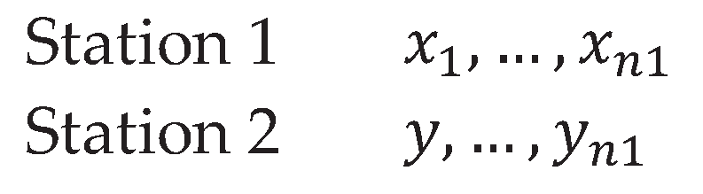
Figure 2.
Maximum bivariate sample arrangement.
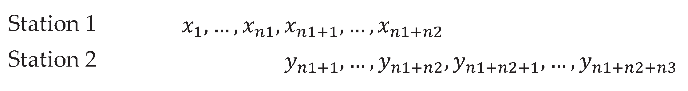
Figure 3.
Methodology of the Flood Frequency Analysis applied in this study.
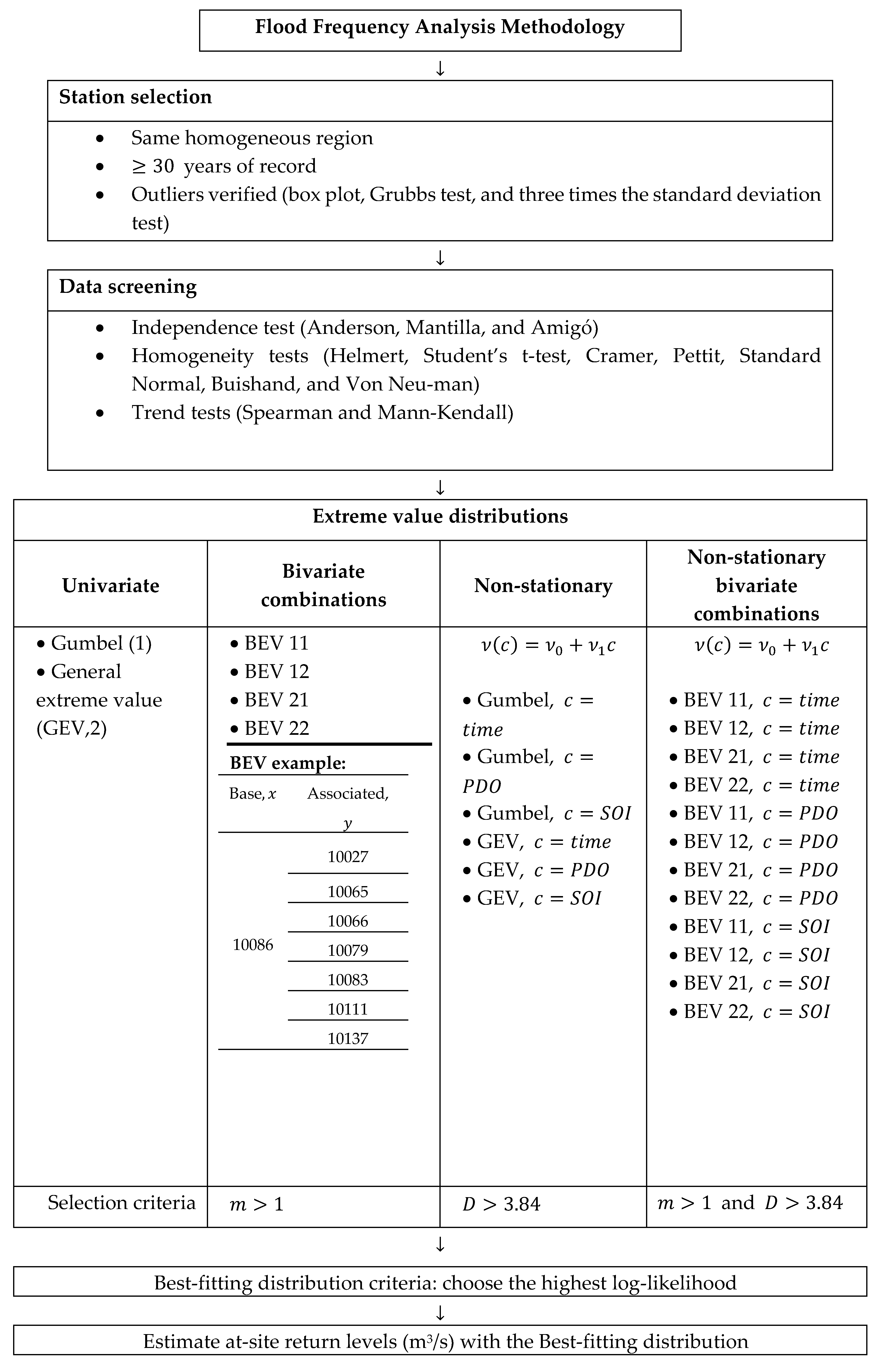
Figure 4.
Maximum instantaneous discharges (m3/s) recorded at Station 10086.

Figure 5.
Return level events (m3/s) for various return periods and scenarios at Station 10086 – non-stationarity BEV 21 and stationarity GEV.
Figure 5.
Return level events (m3/s) for various return periods and scenarios at Station 10086 – non-stationarity BEV 21 and stationarity GEV.
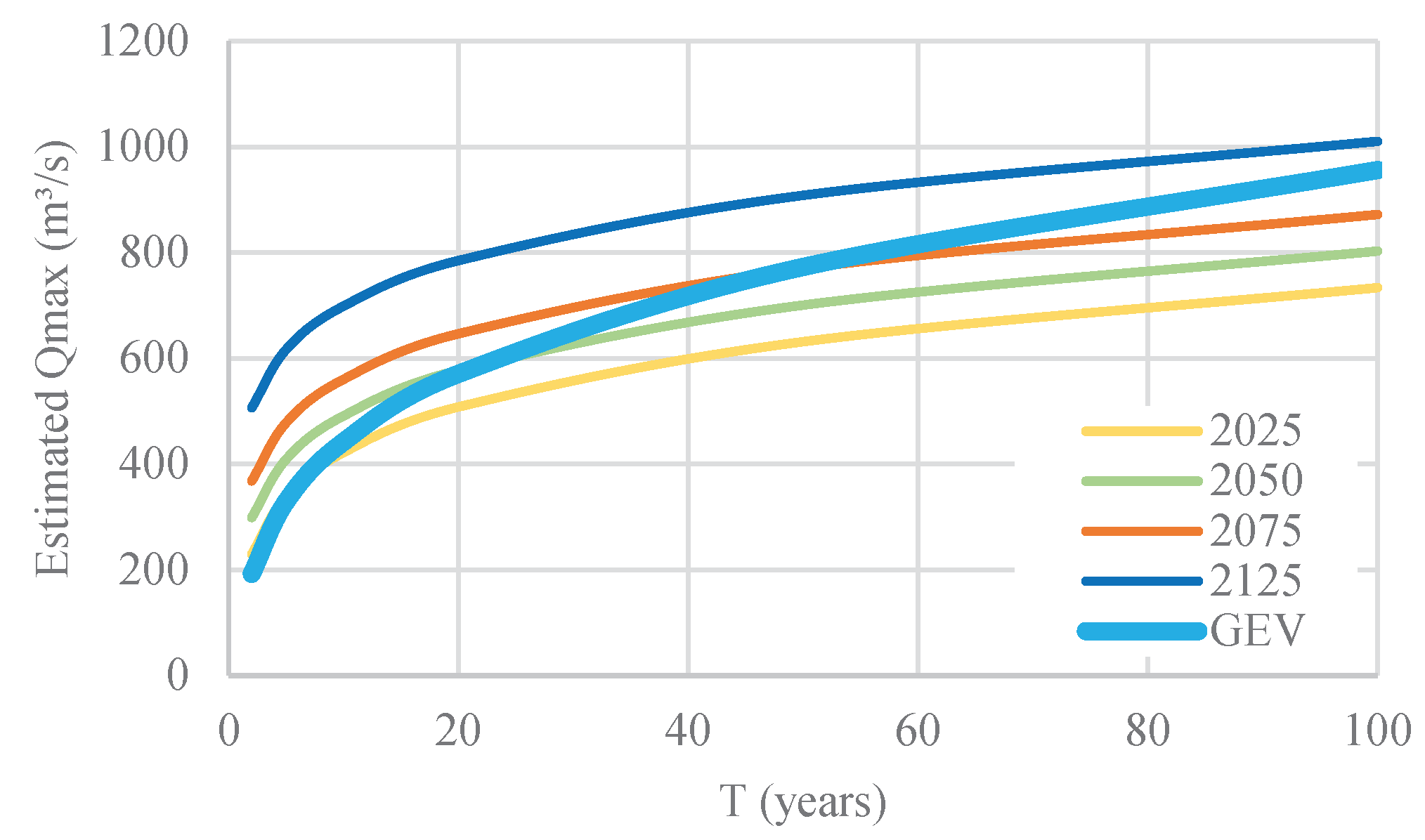

Table 1.
Some characteristics of the stations analyzed.
| Station | Period | Length of record (years) | Mean | Standard deviation |
Kurtosis | Skewness | Variation coefficient |
|---|---|---|---|---|---|---|---|
| 10027 | 1938 - 1995 | 58 | 285.79 | 260.83 | 13.68 | 2.74 | 0.91 |
| 10065 | 1953 - 1999 | 47 | 1218.73 | 1081.76 | 13.59 | 2.84 | 0.89 |
| 10066 | 1955 - 2005 | 51 | 311.89 | 278.67 | 16.36 | 3.18 | 0.89 |
| 10079 | 1959 - 1999 | 41 | 1016.91 | 1642.41 | 19.86 | 3.74 | 1.62 |
| 10083 | 1960 - 1992 | 33 | 458.64 | 425.13 | 5.85 | 1.58 | 0.93 |
| 10086 | 1960 - 1992 | 33 | 236.33 | 156.80 | 4.48 | 1.19 | 0.66 |
| 10111 | 1958 - 2009 | 52 | 1315.93 | 1558.22 | 14.23 | 3.03 | 1.18 |
| 10137 | 1958 - 2008 | 51 | 1058.15 | 992.91 | 7.59 | 2.02 | 0.94 |
Table 2.
Independence, Homogeneity, and Trend Test Results.
| Station | Independent? | Homogeneous? | Trend? | Increasing? |
|---|---|---|---|---|
| 10027 | Yes | Yes | No | Yes |
| 10065 | Yes | Yes | No | No |
| 10066 | Yes | No | No | No |
| 10079 | Yes | Yes | Yes | Yes |
| 10083 | Yes | Yes | No | Yes |
| 10086 | Yes | No | Yes | Yes |
| 10111 | Yes | Yes | No | No |
| 10137 | Yes | Yes | No | No |
Table 3.
Station 10086 distribution results.
| Distribution | Covariate | m | L | D | |||||||
|---|---|---|---|---|---|---|---|---|---|---|---|
| Gumbel | - | - | 168.54 | 108.89 | -203.88 | ||||||
| GEV | - | - | 155.56 | 96.66 | -0.235 | -204.12 | |||||
| BEV 21 -10137 | - | 1.11 | 154.55 | 92.42 | -0.094 | 681.09 | 574.59 | -200.14 | |||
| BEV 21 -10137 | Time | 1.10 | 105.82 | 2.77 | 86.74 | -0.123 | 745.27 | -2.45 | 573.55 | -198.55 | 11.13 |
Table 4.
Return levels in m3/s for station 10086.
| Distribution | Scenario | t | T (years) | |||||
|---|---|---|---|---|---|---|---|---|
| 2 | 5 | 10 | 20 | 50 | 100 | |||
| Gumbel | - | - | 208.45 | 331.86 | 413.58 | 491.96 | 593.42 | 669.44 |
| GEV | - | - | 192.55 | 329.32 | 442.08 | 570.59 | 772.66 | 955.82 |
| BEV 21 -10137 | - | - | 189.01 | 303.43 | 386.20 | 471.27 | 590.31 | 686.62 |
| BEV 21 - 10137 non-stationary in time | 2025 | 66 | 320.99 | 431.32 | 513.29 | 599.33 | 722.62 | 824.71 |
| 2050 | 91 | 390.17 | 500.51 | 582.47 | 668.52 | 791.81 | 893.90 | |
| 2075 | 116 | 459.36 | 569.69 | 651.66 | 737.71 | 861.00 | 963.08 | |
| 2125 | 166 | 597.74 | 708.07 | 790.03 | 876.08 | 999.37 | 1101.46 | |
Table 5.
Best-fitting distribution for each station.
| Station | Best-fitting distribution | Covariate | m | L | |||||||
|---|---|---|---|---|---|---|---|---|---|---|---|
| 10027 | BEV 21 - 10065 | SOI | 1.18 | 165.48 | -4.68 | 112.91 | -0.219 | 825.22 | -75.56 | 584.65 | -369.18 |
| 10065 | BEV 21 - 10027 | Time | 1.15 | 804.27 | -1.31 | 436.67 | -0.191 | 190.17 | -0.06 | 148.03 | -361.49 |
| 10066 | BEV 21 - 10079 | SOI | 1.07 | 192.23 | 4.25 | 103.89 | -0.236 | 527.80 | 26.00 | 637.16 | -320.53 |
| 10079 | BEV 21 - 10066 | Time | 1.10 | 337.40 | 1.80 | 270.49 | -0.478 | 257.48 | -1.57 | 142.75 | -301.79 |
| 10083 | BEV 21 - 10065 | Time | 1.34 | 186.50 | 0.59 | 155.50 | -0.455 | 909.26 | -2.88 | 584.78 | -223.72 |
| 10086 | BEV 21 - 10137 | Time | 1.10 | 105.82 | 2.77 | 86.74 | -0.123 | 745.27 | -2.45 | 573.55 | -198.55 |
| 10111 | BEV 21 - 10065 | Time | 2.05 | 800.38 | -6.16 | 338.99 | -0.485 | 943.79 | -2.84 | 626.07 | -395.48 |
| 10137 | BEV 21 - 10066 | SOI | 1.13 | 512.21 | -44.16 | 344.23 | -0.524 | 215.82 | -4.84 | 146.25 | -389.67 |
Disclaimer/Publisher’s Note: The statements, opinions and data contained in all publications are solely those of the individual author(s) and contributor(s) and not of MDPI and/or the editor(s). MDPI and/or the editor(s) disclaim responsibility for any injury to people or property resulting from any ideas, methods, instructions or products referred to in the content. |
© 2025 by the authors. Licensee MDPI, Basel, Switzerland. This article is an open access article distributed under the terms and conditions of the Creative Commons Attribution (CC BY) license (https://creativecommons.org/licenses/by/4.0/).
Copyright: This open access article is published under a Creative Commons CC BY 4.0 license, which permit the free download, distribution, and reuse, provided that the author and preprint are cited in any reuse.


