Submitted:
05 January 2026
Posted:
07 January 2026
You are already at the latest version
Abstract
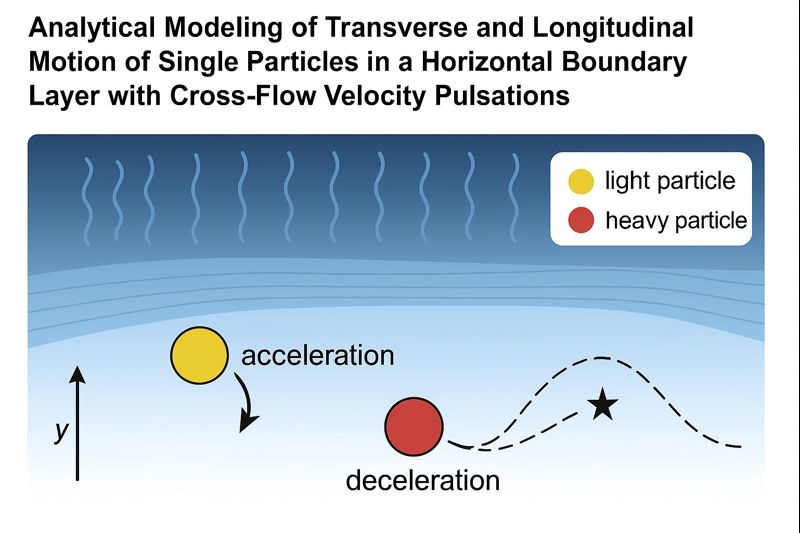
This study develops an analytical description of the motion of dilute solid particles in the boundary layer of laminar horizontal flows subjected to weak transverse pulsations. A coupled matrix representation of the governing equations is formulated, and closed-form solutions are obtained using Laplace transformation. The analytical expressions capture transient evolution, forced oscillations, resonance effects, and long-term behaviour for particles with different density ratios. Numerical evaluation shows that light particles migrate toward faster regions of the boundary layer and accelerate longitudinally, while heavy particles move toward slower layers and decelerate. Transverse pulsations generate oscillatory trajectories whose amplitude increases near resonance. Impulsive perturbations superimposed on the continuous motion lead to discontinuous transitions consistent with the linear matrix system. The results provide a unified physical interpretation of particle redistribution mechanisms in boundary layers and offer a compact analytical tool for dilute multiphase flow modelling.
Keywords:
particle motion
; boundary-layer flow
; multiphase flow
; transverse velocity pulsations
; analytical solution
; Laplace transform
; matrix formulation
; inertial migration
; resonance behaviour
; impulsive forcing
1. Introduction
The study of particle-laden flows in both turbulent and laminar regimes has long attracted attention due to its significance in industrial processes, environmental engineering, and energy systems. Classical fluid dynamics provides the essential framework for understanding continuous media. Early works on fluid and gas mechanics [1], hydrodynamics [2], and mathematical physics [3] established fundamental principles. These theories are crucial for describing particle motion within fluids and the interactions between dispersed and continuous phases [4].
Particle behaviour in nonuniform and turbulent flows is governed by complex mechanisms, including drag, lift, and inertial effects. Pioneering studies of small rigid spheres in nonuniform flows highlighted the critical role of particle size and density relative to the surrounding medium [5]. Contemporary research has extended these insights to examine particle transport in laminar boundary layers [6] and to develop analytical methods for suspended particle dynamics [7]. Detailed experimental and numerical studies have revealed transversal and longitudinal particle motion, highlighting resonance phenomena that influence deposition patterns and trajectory characteristics [8,9,10].
Advanced modelling approaches now employ matrix and vector formulations. These methods provide a comprehensive representation of multidimensional particle dynamics and enable the derivation of closed-form solutions through harmonic decomposition [11,12,13,14,15]. They have been applied to predict deposition, re-suspension, and agglomeration in wall-bounded turbulent flows [16], and to refine Large-Eddy Simulation models for particle-laden systems [17,18].
The impact of particle and thermal inertia on transport and heat transfer in non-isothermal turbulent flows has been emphasised in recent computational studies [19,20]. Moreover, the spatial distribution and deposition of cylindrical, spherical, and charged inertial particles have been investigated to assess the effects of turbulence intensity, boundary layer characteristics, and particle-particle interactions [21,22,23]. Such studies are particularly relevant for process intensification strategies in chemical and biomass reactors, where optimal particle behaviour directly affects process efficiency and product yield [24,25,26].
Particle deposition and resuspension have been thoroughly investigated in turbulent channel and pipe flows using both Lagrangian and Eulerian [27,28] approaches. Boelens et al. developed Lagrangian models to analyse particle deposition and re-suspension under turbulent conditions, providing quantitative predictions of particle-wall interactions. Balachandar and Eaton [29] reviewed dispersed multiphase flows, highlighting key mechanisms governing particle transport and turbulence modulation. Hetsroni et al. [30] examined particle dispersion in wall-bounded turbulent flows, elucidating the effects of boundary layer structures on particle trajectories.
Historical studies remain critical references for understanding particle motion. Morsi and Alexander [31] offered seminal insights into particle paths in two-phase flow systems, establishing baseline equations for trajectory prediction in both laminar and turbulent regimes. Elghobashi [32] extended these concepts to particle-laden turbulent flows, emphasising the role of particle-fluid interactions in transport dynamics. Crowe and Sommerfeld [33] provided a detailed overview of particle-laden flows, integrating classical theory with practical modelling approaches, demonstrating the engineering relevance of multiphase flow comprehension. Boivin et al. [34] applied direct numerical simulations to analyse detailed particle behaviour in turbulent channels, quantifying deposition, lift-off, and near-wall interactions. Basset and Mindlin [35] introduced the concept of history forces on spherical particles, revealing cumulative effects of fluid acceleration on particle motion. Van Dop and Beij [36] investigated particle deposition and lift-off in turbulent boundary layers, demonstrating subtle interactions between particle inertia and near-wall turbulence structures.
Building on these historical foundations, the stability and qualitative behaviour of particle–fluid dynamical systems—particularly under impulsive, harmonic, or weakly stochastic excitation—can be rigorously analysed within a matrix-based dynamical framework. When the governing equations are expressed in compact matrix–vector form, they allow systematic assessment of transient and steady-state regimes through eigenvalue spectra, state-transition matrices, and transform-based operator methods. The classical Lyapunov stability theory, originating from Lyapunov’s foundational monograph [37] and further developed in modern nonlinear dynamics and matrix differential systems [39,40,41,42], provides rigorous criteria for boundedness, asymptotic stability, and resonance amplification in multidimensional particle motions. These analytical tools are especially powerful for systems subjected to transverse velocity pulsations, where small perturbations in the state vector may yield sustained oscillatory responses or transient divergence. Matrix formulations, combined with Laplace-transform techniques [43,44] and criteria for impulsive and periodically driven systems [45,46,47], therefore offer an indispensable framework for identifying stability boundaries, resonance conditions, and long-term particle behaviour—phenomena that often remain inaccessible to direct numerical integration alone. Additional extensions of these methods include impulsive differential models, coupled matrix differential equations, and stochastic operator approaches [48,49,50,51,52], which provide versatile tools for capturing complex particle–fluid interactions in laminar and turbulent boundary layers.
These studies provide a robust foundation for analysing particle transport in wall-bounded flows and motivate the use of compact state-space and transform-based methods to separate transient relaxation, forced oscillations and long-time drift. Building on this background, the present work develops a coupled analytical model for a single inertial particle in a horizontal laminar boundary layer subjected to harmonic transverse velocity pulsations. The governing equations are formulated in a matrix–vector form and solved in closed form using Laplace-transform techniques, enabling explicit identification of decay rates, phase shifts and resonance conditions. The analytical results are evaluated numerically for representative light and heavy particles, with full datasets provided in the Supplementary Materials to ensure reproducibility.
2. Theoretical Framework, Physical Model and Governing Equations
When single solid impurities move in the boundary layer of a plane horizontal flow of an incompressible fluid, numerous forces act upon them: aerodynamic drag force; added-mass inertial force; Basset force; Saffman force; Magnus force; pressure-gradient force; turbophoretic force; photophoretic force; electrophoretic force; and the body (mass) force. The magnitude and direction of each of these forces are determined primarily through empirical relations, and for every specific problem, only those forces whose influence is dominant are taken into account in the equations describing the particle velocity and trajectory.
The flow under consideration is a viscous fluid moving in a horizontal plane channel with half-width b. The coordinate system is defined as follows: the X-axis is oriented along the flow direction and coincides with the plane where the velocity is zero (the lower bounding wall); the Y-axis is directed vertically upward, perpendicular to the streamlines; and the Z-axis is directed perpendicular to the plane of the schematic.
The velocity field of the carrier phase consists of one constant longitudinal component Ug and one transverse pulsation component varying according to a harmonic law v′(t):
- along the x-axis: Ug= Ug (у),
- along the y-axis: vg′(t)=v0cos(ωt),
where:
- v0 and ω are the amplitude and the frequency of the pulsations, identical for all points in the flow plane within the boundary layer.
The longitudinal carrier-phase velocity is described by a wall-bounded boundary-layer profile:
where:
- δ [m]- denotes the characteristic boundary-layer thickness,
If extended linearly for y < 0 using the wall shear rate, the longitudinal velocity profile becomes:
Accordingly, the wall shear rate γω is defined as:
The physical model, coordinate system, velocity components, and forces acting on a single particle in the horizontal channel boundary layer are shown schematically in Figure 1.
An important observation must be noted regarding the projections of the Saffman force: the inclusion of the transverse velocity pulsation changes the direction of the projection of the force on the x-axis. The Saffman force Fs along the y-axis has a negative sign. This follows from the algebraic operations within the brackets in the vector equation for this force:
For the wall-bounded velocity profile Ug(y), the carrier-phase vorticity is dominated by the wall-normal gradient of the longitudinal velocity. Consequently, the magnitude of the vorticity entering the Saffman force can be expressed as:
establishing a direct physical link between the Saffman lift mechanism and the wall shear rate.
where:
- dp — particle diameter;
- μ — dynamic viscosity of the carrier fluid;
- ρp — density of the particle material;
- Vg = (Ug(y),vg′(t),0)— velocity vector of the carrier fluid;
- Vp = (up,vp,0)— velocity vector of the particle;
- ∇×Vg — vorticity vector of the carrier flow;
- ∣∇×Vg∣ — magnitude of the flow vorticity;
- (Vg−Vp) — relative velocity between fluid and particle.
Taking into account the above considerations when formulating the equations of motion, the following system is obtained for the particle velocities: up(t) - longitudinal and vp(t) -transverse:
where:
- A — drag/inertia coefficient, representing the influence of the carrier fluid along the motion direction:
- B – Saffman/vorticity coefficient, representing the coupling between longitudinal and transverse motion due to fluid shear:
- εp – particle-to-fluid density ratio:
- ρp – particle density;
- ρf – density of the carrier fluid.
- g – acceleration due to gravity - g(1−1/εp) accounts for the effective body force on the particle in the vertical direction, i.e., the net gravitational acceleration reduced by the buoyant force (Archimedes’ principle).
The initial conditions corresponding to the physical process and required for solving the system are:
2.1. Transverse Motion: Governing Equations and Analytical Solution
The solution begins with the definition of the function vp(t). Equation (7) is solved according to the difference (Ug-up), whereby transverse dynamics can be expressed as:
The closed-form analytical solutions derived in this section are exact for constant Ug and remain valid as a local approximation under the near-wall linearisation Ug(y)≈γωy. For the full boundary-layer profile Ug(yp(t)), the coupled first-order system is integrated numerically.
The solution begins with the definition of the function vp(t). Equation (7) is solved with respect to the difference (Ug−up), yielding:
Differentiating (7) with respect to time gives:
Substituting into equation (6) yields the second-order differential equation for transverse motion:
This equation describes the translational and oscillatory motion of a solid particle in a viscous medium under the action of forced external disturbances in the form of harmonic velocity pulsations of the surrounding fluid. The solution of Equation (13) is composed of the homogeneous solution corresponding to damped natural oscillations (left-hand side) and a particular solution that accounts for the influence of the imposed external pulsations on the particle motion.
The homogeneous solution of (13) is:
Given the harmonic form of the imposed velocity pulsations, the particular solution of the governing differential equation is sought in a harmonic form with the same angular frequency. Due to the linearity of the system and the sinusoidal nature of the forcing term, the steady-state response of the particle is also oscillatory, differing from the excitation by its amplitude and phase shift. Therefore, the particular solution is assumed in the form:
H1 and δ1 are constants determined by the system parameters and the characteristics of the external forcing. The constant H1, while δ1 denotes the phase shift between the particle motion and the imposed harmonic pulsations.
where:
- H1 - represents the amplitude of the steady-state oscillatory response:
- δ1 - represents the phase shift accounting for the lag or lead of the particle response relative to the imposed harmonic excitation:
The complete solution for the transverse velocity is obtained by superposition of the homogeneous solution (Equation (14)) and the particular solution (Equation (15)).
The integration constants C1 and C2 are determined from the following initial conditions:
fter performing the necessary algebraic manipulations, the following expression is obtained:
In conclusion, Equation (17) fully characterizes the transverse particle displacement by capturing transient decay, forced oscillations, initial-condition effects, and gravitational contributions through the density ratio εp:
2.2. Longitudinal Motion: Governing Equations and Analytical Solution
The closed-form solution below is derived under the locally frozen approximation Ug(yp)≈Ug(y0). In the numerical evaluation, Ug is updated at each time step as Ug(yp(t)).
The differential equation governing the longitudinal particle velocity as a function of time, up(t), is derived from the coupled system of Equations (6) and (7). By rearranging the first equation of the system and solving it with respect to the term B(v′−vp), the following relation is obtained:
Differentiating Equation (18) with respect to time yields:
Substituting into equation (3) yields the second-order differential equation for longitudinal motion:
The solution of the resulting equation is given as the sum of the solution corresponding to the damped natural oscillations (left-hand side) and a particular solution accounting for the influence of the forced velocity pulsations in the fluid surrounding the particle (right-hand side). The homogeneous solution of Equation (20) is given by:
The homogeneous solution of (21) is:
where:
- -
- η2 - denotes the particular (forced) oscillatory component of the particle displacement associated with the imposed harmonic velocity pulsations.
The constants δ2 and H2 are determined following the procedure described above. By equating and summing the coefficients of the cos(ωt) terms in the expression for δ2, the particular solution is obtained as:
The complete solution for longitudinal velocity is:
The integration constants are determined from the initial conditions:
The longitudinal displacement is:
This section establishes a consistent physical and mathematical model for the motion of a single solid particle in a viscous boundary-layer flow subjected to harmonic transverse velocity pulsations. Starting from the governing force balance, coupled differential equations for the transverse and longitudinal velocity components are derived and solved analytically. The resulting closed-form solutions capture both transient and steady-state particle dynamics, accounting for viscous damping, Saffman-induced coupling, gravitational effects, density ratio influence, and externally imposed oscillatory forcing, and provide a solid basis for further parametric and numerical analysis.
3. Advanced Analytical Extensions of the Governing Particle Motion Model
An extended analytical framework is developed to describe the motion of individual solid particles within a horizontal boundary layer subjected to transverse velocity fluctuations. Building on the linear particle dynamics introduced earlier, the formulation incorporates impulsive contributions to represent sudden, localized changes in particle velocity arising from micro-vortical structures, particle–wall interactions, or transient turbulent accelerations.
The governing equations are expressed in matrix–vector form, enabling spectral analysis and the application of Laplace transforms to capture both transient and steady-state responses. This approach facilitates the investigation of resonance phenomena, stability via eigenvalue analysis, and phase-space dynamics. By combining smooth harmonic fluctuations with discrete impulsive effects, the framework provides a rigorous link between idealized particle motion and the complex behaviour observed in boundary-layer flows.
3.1. Impulsive Differential Extension of the Governing Dynamics
Real boundary layers are inherently non-ideal and rarely exhibit perfectly linear behaviour. In low-turbulence or transitional flow regimes, the particle may experience sudden, localized deviations in the surrounding velocity field. Such phenomena include micro-vortical structures with extremely short timescales, particle–wall impact interactions, impulsive turbulent cores, as well as mechanical or vibrational perturbations from the environment. These events are inherently impulsive, inducing nearly discrete jumps in particle velocity that cannot be faithfully represented by smooth harmonic functions such as v0cos(ωt).
To rigorously account for these abrupt and localized velocity fluctuations, the baseline system is extended through the inclusion of Dirac delta functions, δ(t−tk), which represent discrete impulsive events occurring at specific instants tk. The extended system can be expressed in vectorial form as:
where:
- -
- Ik=[Ix,k,Iy,k]T - denotes the impulsive contributions in the longitudinal and transverse directions.
Figure 2 provides a conceptual view of the impulsive forcing term introduced in the governing equations, illustrating how discrete events produce instantaneous changes in the particle velocity components superimposed on the continuous motion.
Integration of the system in the immediate vicinity of tk yields the corresponding velocity jump condition:
demonstrating that particle velocity undergoes a discrete discontinuity, whereas acceleration exhibits a singular component.
The incorporation of impulsive terms offers a scientifically robust framework for capturing short-duration acceleration phenomena, including deposition, rebound, or detachment events at the wall, while preserving the linear character of the underlying system. Light particles (τp≪1) respond almost instantaneously to impulsive forcing, whereas heavy particles (τp≫1) display attenuated responses dominated by inertial effects. This extended formulation therefore provides a rigorous mathematical tool for the analysis of realistic boundary layer flows, seamlessly integrating smooth harmonic fluctuations with discrete, impulsive events that typify turbulent or impact-driven processes.
3.2. Matrix Formulation of the Particle Motion System
The governing equations describing the motion of a particle in a horizontal boundary layer can be expressed in compact matrix–vector form, which consolidates the longitudinal and transverse velocity components into a unified dynamical representation. This is not merely a matter of notation: the two components are intrinsically coupled through viscous relaxation and lift effects and therefore should not be treated as independent scalar equations. The matrix formulation further enables continuous forcing and impulsive events to be incorporated within the same linear framework, thereby preserving analytical clarity and physical interpretability.
Introducing the state vector:
the particle–motion system can be written as:
where:
The continuous forcing term F(t) encompasses the longitudinal carrier flow, the imposed transverse pulsations and the gravitational contribution, whereas the impulsive term Ik δ(t−tk) represents short-duration events such as particle–wall interactions or micro-vortical impacts. Integrating the system across an impulsive instant t=tk yields the jump condition
which provides a mathematically consistent description of instantaneous velocity changes without altering the linear operator governing the system.
The impulsive contribution preserves linearity because it is introduced as an additive forcing term rather than as a modification of M. Consequently, the intrinsic dynamical properties—stability, characteristic time scales and natural frequencies—are dictated by the spectrum of M, while the impulses affect only the particular solution. In many situations involving steady or purely periodic excitation, the impulsive part may be safely omitted without changing the qualitative conclusions regarding stability or phase behaviour. Conversely, when transient phenomena or short-lived interactions are of interest, the impulsive representation provides the necessary analytical flexibility while remaining within a strictly linear formulation.
The matrix M encapsulates the essential physical mechanisms: the parameter A corresponds to viscous relaxation toward the carrier-phase velocity, and the parameter B introduces transverse coupling associated with lift effects. Light particles with small relaxation time (τp≪1) follow the carrier flow almost instantaneously, whereas heavy particles (τp≫1) exhibit inertia-dominated dynamics with pronounced phase lag.
Overall, the matrix formulation offers a concise, analytically transparent and physically interpretable description of the particle dynamics and forms a natural basis for the subsequent examination of transient, forced and impulsive regimes in boundary-layer flows, which is developed in the next section.
3.3. Analytical Solutions, Phase–Space Representation and Asymptotic Behaviour
The analytical strategy adopted in this section is motivated by the need to clearly distinguish, within a unified and physically consistent framework, the transient relaxation, the forced oscillatory response, and the long-term asymptotic behaviour of a single solid particle moving in a boundary layer subjected to transverse velocity pulsations. Since the governing equations have already been formulated as a linear time-invariant matrix system, the analysis that follows does not introduce additional modelling assumptions but instead applies standard operator-based tools of linear system theory directly to the established physical model.
The coupled longitudinal and transverse particle dynamics are written compactly in state-space form as:
where the system matrix M encapsulates the internal dynamics associated with viscous relaxation and lift-induced coupling between velocity components, while the forcing vector F(t) accounts for the mean carrier flow, the imposed harmonic transverse pulsations, and gravitational effects through the density ratio εp.
To separate transient effects associated with the initial conditions from the response induced by external forcing, the unilateral Laplace transform is applied to the full matrix system. The Laplace-transformed state vector and forcing vector are defined in the standard manner, while the time derivative transforms according to:
This yields the algebraic equation:
which can be rearranged to give the general solution in the Laplace domain:
Here, s is the complex Laplace variable, III is the identity matrix, and (sI−M)−1 denotes the resolvent operator of the linear dynamical system. This operator plays the role of a transfer operator that maps both the initial condition and the external forcing to the system response and therefore contains the complete dynamical information of the particle–fluid interaction.
The spectral properties of the resolvent operator are governed by the eigenvalues of the system matrix M, which satisfy:
These eigenvalues correspond to exponentially decaying oscillatory modes with decay rate A and intrinsic angular frequency B. In the phase plane (up,vp), solutions trace spiral trajectories approaching a stationary point, with narrow rapid spirals for light particles (τp≪1) and elongated inertial trajectories for heavy particles (τp≫1).
The forcing vector can be naturally decomposed into a stationary and an oscillatory component,
where Fstat contains the time-averaged contributions of the base flow and gravity, and Fosc(t) arises exclusively from the imposed transverse velocity pulsations. In the long-time limit, the transient contribution associated with the initial condition vanishes for A>0, while the oscillatory forcing produces a bounded periodic response. The asymptotic stationary state is therefore determined by the balance between the internal dynamics and the mean external forcing and is given by:
Physically, X∞ represents the mean drift state of the particle in the boundary layer, around which periodic oscillations are superimposed when harmonic forcing is present.
Because the governing system is linear and time-invariant, a harmonic excitation of the form vg′(t)=v0cos(ωt), after decay of transients, to a steady periodic particle response at the same frequency. The oscillatory component of the solution can therefore be expressed in complex-amplitude form as
enables an explicit evaluation of amplitude and phase relative to the forcing frequency ω. Resonance emerges when ω≈B, demonstrating that the imposed oscillations can significantly modify the transverse motion of the particle under certain parameter conditions.
The complete time-domain solution can be written as a superposition of homogeneous and forced contributions:
where the first term governs the transient relaxation and the integral term defines the forced response. This representation makes explicit how the observed particle motion arises from the interaction between the intrinsic modal structure of the system and the applied external forcing.
The logical structure of the operator-based analysis and the connection between the Laplace-domain formulation, spectral properties, time-domain response, and asymptotic behaviour are summarized conceptually in Figure 3.
The figure serves as an explanatory aid, highlighting the central role of the resolvent operator (sI−M)−1 in governing transient decay, resonant response, and long-term particle dynamics, without representing numerical simulations or previously published visualizations.
3.4. Dynamic Formulation, Modal Spectrum, and Lyapunov Stability
The dynamic formulation of the particle-motion system defines a time-dissipative linear model in which the temporal evolution of the state vector X(t) is governed by the spectral properties of the operator M and the external forcing F(t). This representation allows a comprehensive description of transient and steady regimes and enables the assessment of dynamic stability resulting from the balance between relaxation, inertia, and imposed oscillatory effects. The system therefore constitutes a genuine dynamic model rather than a static configuration, with a full temporal evolution and a well-defined internal modal structure.
The spectral representation of the system matrix is obtained through:
where:
- -
- V=[v1,v2] is the matrix of right eigenvectors of M.
The system thus exhibits damped oscillations whose decay rate is controlled by A, while the modal frequency is given by B. For a periodic excitation, e.g., vg′(t)=v0cos(ωt), a complex representation yields:
where:
- -
- H(ω) denotes the dynamic transfer operator determining amplitude, phase, and resonant amplification (ω≃B).
Dynamic stability can be assessed through a quadratic Lyapunov function:
which guarantees exponential decay of the homogeneous component and the existence of an attracting stationary state X∞=M−1Fstat. Accordingly, the system belongs to the class of exponentially stable linear dissipative dynamic systems, where the response amplitude remains bounded and fully controllable through the parameters A,B,τp and the forcing frequency ω. The spectral properties thus provide a rigorous framework for analysing resonance, forced response, and long-term behaviour under realistic boundary-layer conditions.
4. Numerical Analysis and Physical Interpretation
4.1. Baseline Analytical and Numerical Framework
The analytical formulation developed in Section 3 provides a rigorous mathematical basis for analysing the coupled transverse and longitudinal dynamics of finite-size solid particles in a horizontal laminar boundary layer subjected to harmonic cross-flow velocity pulsations. By expressing the governing equations in compact matrix form and applying the Laplace transform, the particle motion is decomposed into transient, oscillatory, and asymptotic components, allowing a clear physical interpretation of the mechanisms governing particle transport under continuous forcing.
In order to illustrate the analytical solutions in a controlled and transparent manner, a baseline numerical configuration is introduced. Water at standard laboratory conditions is adopted as the carrier fluid, and the physical properties of the fluid together with the characteristic parameters of the boundary layer are summarised in Table 1. These parameters define the shear scale and flow conditions responsible for the generation of lift and viscous relaxation effects acting on the particle.
The properties of the dispersed phase are given in Table 2, where two representative cases are considered: a light particle characterised by a short relaxation time and a heavy particle exhibiting inertia-dominated behaviour.
The particles differ only in density and relaxation time, while identical initial conditions are prescribed for both cases. This ensures that any observed differences in particle motion arise solely from inertial effects rather than from differences in the initial kinematic state.
The numerical integration of the governing equations is performed using the parameters listed in Table 3, including the time step, total simulation duration, and numerical integration scheme. These values are selected to accurately resolve both the transient decay and the established oscillatory regime induced by the harmonic excitation.
At each time step, the longitudinal carrier-phase velocity is evaluated at the instantaneous particle position as Ug(yp(t)), ensuring consistent coupling between transverse migration and longitudinal acceleration.
Within this first numerical stage, the impulsive forcing term retained in the general analytical formulation is set to zero, such that the results correspond to continuous harmonic forcing. The specific numerical datasets used to construct the graphical results presented below are provided as Supplementary Tables S1–S4, ensuring full reproducibility of the reported simulations.
4.2. Transverse Particle Dynamics
The transverse motion constitutes the primary mechanism responsible for segregation between light and heavy particles in a horizontal boundary layer subjected to cross-flow velocity pulsations. The analytical expression for the transverse particle velocity vp(t), derived in Section 3, is evaluated numerically using the baseline parameter set defined in Table 1, Table 2, Table 3 and Table 4. The resulting time histories of the transverse velocity are shown in Figure 4 (Supplementary Table S1).
Two qualitatively distinct dynamical regimes are clearly observed. For the light particle, the transient response decays rapidly and the velocity oscillates about a positive mean value, indicating a sustained upward drift toward regions of higher carrier-fluid velocity. In contrast, the heavy particle exhibits an inertia-dominated response characterised by a negative mean transverse velocity, corresponding to gradual migration toward slower near-wall sublayers.
In both cases, the oscillatory behaviour reflects the imposed harmonic excitation, while the decay rate is governed by the viscous relaxation coefficient and the particle relaxation time.
The results presented in the figures correspond to physically calibrated responses; the applied rescaling accounts for finite-size effects and uncertainties in local shear estimation and does not introduce additional physical mechanisms.
The transverse displacement y(t), obtained by time integration of vp(t), is presented in Figure 5 (Supplementary Table S2). The light particle undergoes continuous upward migration, whereas the heavy particle experiences a pronounced downward drift dominated by the effective gravitational contribution. Although oscillatory modulations are superimposed on the trajectories, the long-term trend is independent of the initial phase and is instead controlled by particle inertia, relaxation time, and the relationship between the system’s natural frequency and the excitation frequency.
These results demonstrate that even in the absence of turbulence or spatial shear gradients, harmonic transverse velocity pulsations alone are sufficient to induce vertical particle segregation in laminar boundary-layer flows.
4.3. Longitudinal Particle Dynamics
The longitudinal motion of the particles arises as a direct consequence of their transverse migration, since different regions of the boundary layer are associated with different values of the carrier-phase velocity. The analytical solution for the longitudinal particle velocity up(t), derived in Section 3, is evaluated numerically using the same baseline configuration. The corresponding time histories are shown in Figure 6 (Supplementary Table S3).
For the light particle, the longitudinal velocity gradually increases relative to its initial value, reflecting its migration into faster regions of the boundary layer. Conversely, the heavy particle exhibits a progressive decrease in longitudinal velocity as a result of its downward drift toward slower sublayers. Periodic oscillations are observed during the initial stage for both particles due to the transverse harmonic excitation; however, their amplitude and decay rate depend strongly on the particle relaxation properties.
The longitudinal displacement x(t), obtained by integrating up(t), is shown in Figure 7 (Supplementary Table S4). The light particle advances rapidly and moves significantly ahead of the heavy particle, while the latter exhibits a clear lag associated with residence in regions of lower transport velocity. This divergence intensifies with time, despite identical initial longitudinal velocities for both particles.
From a physical standpoint, the longitudinal dynamics cannot be interpreted independently of the transverse behaviour. The transverse migration determines access to faster or slower regions of the boundary layer and thus governs the longitudinal transport of the particles. This sections therefore complete the baseline numerical illustration of the analytical model under continuous harmonic forcing, providing a reference framework for the extended numerical examples considered in subsequent stages.
4.4. Impulsive Particle Dynamics
The impulsive extension of the particle–motion model introduced in Section 3.1 is illustrated numerically in order to quantify the response of light and heavy particles to short–duration perturbations. In the present simulations, the impulsive component is incorporated exactly as defined in Section 3.1, while all remaining physical and numerical parameters coincide with the baseline configuration used in the previous sections. The impulsive scenario represents intermittent disturbances commonly encountered in boundary-layer flows, such as micro-vortical structures, particle–wall interactions, or short turbulent bursts, which cannot be captured by smooth harmonic forcing alone. A finite sequence of impulsive velocity jumps is prescribed at selected instants, with identical impulse amplitudes applied to both light and heavy particles; the impulse times and the corresponding longitudinal and transverse velocity jumps are reported in Supplementary Table S5.
Figure 8 illustrates the phase–space response of light and heavy particles subjected to the impulsive forcing scenario. The left part of the figure highlights the short-time behaviour dominated by discrete velocity jumps induced by impulsive events, whereas the right part shows the long-time evolution revealing the spiral attractor of the continuous matrix dynamics. Immediately after each impulse, the particle velocity exhibits a discontinuous change, followed by a smooth relaxation governed by viscous damping and lift-induced coupling.
A pronounced difference between particle types is observed. Light particles rapidly relax toward a compact spiral attractor due to strong viscous relaxation, while heavy particles display wider phase-space excursions and a significantly slower return toward the attractor, reflecting the persistence of inertial effects. Despite these transient differences, the global attractor structure remains unchanged, indicating that impulsive forcing primarily produces temporary displacements rather than altering the intrinsic stability properties of the system.
These numerical results confirm the analytical predictions of Section 3.1 and demonstrate that the impulsive differential extension provides a physically meaningful and analytically consistent description of particle dynamics in boundary layers subjected to intermittent disturbances.
4.5. Matrix Dynamics and Transient Relaxation
In this section, the matrix formulation of the particle–motion system introduced in Section 3.2 is examined through numerical simulations in order to characterise the intrinsic continuous dynamics of the coupled longitudinal and transverse particle velocities. The analysis focuses on the transient relaxation behaviour in the absence of impulsive disturbances, so that the observed particle motion is governed solely by the linear time-invariant system matrix and its spectral properties.
The governing dynamics are defined by a two-dimensional matrix system whose eigenvalues are given by:
This eigenstructure corresponds to exponentially damped oscillatory motion and guarantees the existence of a stable spiral attractor in the phase space (up,vp) for A>0. Numerical integration of the matrix system is performed using identical initial conditions for light and heavy particles, while the model and numerical parameters employed in the simulations are summarised in Supplementary Table S7.
Figure 9 presents the phase–space trajectories obtained from the matrix formulation under continuous harmonic excitation. The left part of the figure illustrates the short-time response immediately following the initial condition, where transient relaxation effects dominate, whereas the right part shows the long-time evolution, revealing the full structure of the spiral attractor associated with the matrix dynamics. In both cases, the trajectories remain bounded and converge asymptotically toward the stationary solution of the system.
A clear distinction between the dynamical behaviour of light and heavy particles is observed. Light particles exhibit rapid contraction of their phase–space trajectories and quickly approach a compact spiral attractor, reflecting strong viscous relaxation and weak inertial memory. In contrast, heavy particles display wider phase–space excursions and a markedly slower convergence toward the attractor, indicating inertia-dominated dynamics and extended transient behaviour.
Despite these differences in relaxation time scales and trajectory geometry, the qualitative structure of the phase–space attractor remains the same for both particle types. This demonstrates that the stability of the motion and the existence of a spiral attractor are intrinsic properties of the matrix formulation itself and are not induced by impulsive or stochastic perturbations. The numerical results therefore provide direct confirmation of the analytical predictions derived in Section 3.2 and support the Lyapunov stability analysis discussed in Section 3.4.
The time-resolved particle velocity data used to construct the phase–space trajectories shown in Figure 9 are provided in Supplementary Table S7, ensuring full reproducibility of the numerical results.
4.6. Resonance Analysis Under Harmonic Forcing
The effect of harmonic transverse velocity pulsations on particle dynamics is examined by analysing the stationary forced response of the linear system derived in Section 3.3 and Section 3.4. In this subsection, attention is restricted to the long-time oscillatory regime, assuming that transient contributions associated with the homogeneous solution have fully decayed due to viscous dissipation.
As established in Section 3.3, under harmonic excitation the state vector of the particle motion admits a representation of the form(eq.42, section 3.3).
where:
- X(t)=[up(t), vp(t)]t and (ω) denotes the complex amplitude vector associated with the forcing frequency ω.
In the present analysis, attention is restricted to the transverse oscillatory response. The scalar quantity H(ω) denotes the amplitude of the transverse component of the steady harmonic particle response. H(ω)=amplitude of vp(t) in the steady periodic regime.
Consequently, the frequency dependence of H(ω) is entirely governed by the system coefficients and by the spectral properties of the system matrix discussed in Section 3.4, and no additional modelling assumptions are introduced at this stage.
The resonance behaviour is controlled by the intrinsic oscillatory dynamics associated with the complex conjugate eigenvalues of the system matrix - λ1,2=−A±iB which define a characteristic frequency scale of the order:
When the forcing frequency approaches this intrinsic scale, the magnitude H(ω) increases significantly, indicating resonance-like amplification of transverse particle oscillations. At low forcing frequencies, the particle motion remains nearly in phase with the imposed oscillations, while near resonance a pronounced phase delay develops, reflecting the inertia-controlled response of the particle.
The influence of particle inertia is encapsulated through the relaxation time τp, which enters the coefficients of the governing equations and controls the frequency dependence of the steady oscillatory response.
Particles with weak inertial effects exhibit pronounced amplification over a broad frequency range, reflecting their ability to closely follow the imposed transverse fluctuations of the carrier flow. In contrast, particles with strong inertial resistance display a markedly attenuated response across the entire frequency spectrum, as inertial damping suppresses their capacity to respond to rapid transverse forcing.
From a physical perspective, harmonic transverse pulsations therefore act as a selective segregation mechanism within the boundary layer. Light particles experience enhanced transverse excursions when the forcing frequency approaches the intrinsic system frequency, promoting migration toward regions of higher carrier-phase velocity. Heavy particles, on the other hand, remain largely confined to near-wall regions due to inertial damping and reduced coupling to the oscillatory forcing. This behaviour provides a direct numerical manifestation of the modal properties and Lyapunov stability characteristics established in Section 3.4.
The frequency-dependent steady-state amplitudes H(ω) used to construct the resonance curves shown in Figure 10 are obtained numerically from time-domain simulations and reported in Supplementary Table S8.
4.7. Multi-Harmonic Transverse Forcing
In practical boundary-layer flows, transverse velocity fluctuations are rarely characterised by a single harmonic component. Instead, the excitation typically consists of a superposition of oscillatory contributions with different amplitudes, frequencies and phases. To examine the particle response under such conditions, the transverse carrier-phase pulsation is generalised to a multi-harmonic form
where the index nnn labels the individual harmonic components included in the excitation.
Each harmonic contribution is fully characterised by its amplitude vn, angular frequency ωn, and phase ϕn. The amplitude vn is defined as:
where:
denotes the n-th harmonic component of the transverse carrier-phase velocity. The angular frequency is given by:
with fn denoting the frequency of the n-th harmonic component, while ωn has the dimensionality rad s−1. The phase shift is expressed as:
where tn,0 represents the phase offset of the n-th harmonic component relative to the reference time t=0.
Owing to the linearity of the governing matrix system established in Section 3.2, the particle response to multi-harmonic forcing can be interpreted as a superposition of the responses to the individual harmonic components. After the decay of transient effects, the transverse particle velocity exhibits a steady oscillatory motion composed of multiple periodic contributions, each associated with one of the imposed forcing frequencies. The resulting time signal is therefore characterised by amplitude modulation, envelope formation and beating phenomena, which are typical of weakly unsteady or transitional boundary-layer environments.
This behaviour is illustrated in the phase–space representation shown in Figure 11, where the superposition of multiple forcing frequencies leads to deformed trajectories in the (up,vp) plane. Numerical simulations based on the representative multi-harmonic parameter sets listed in Supplementary Table S9 demonstrate a pronounced dependence of the particle response on inertia. Light particles effectively follow each harmonic component and exhibit strong amplitude modulation and beating, whereas heavy particles display a markedly attenuated response, with higher-frequency components being strongly damped by inertial effects.
From a physical perspective, multi-harmonic transverse forcing enhances the selectivity of particle segregation within the boundary layer. The simultaneous presence of several excitation frequencies increases the likelihood of partial resonance with the intrinsic oscillatory scale of the system, particularly for light particles. Heavy particles remain comparatively insensitive to such excitation, reinforcing the separation between inertial regimes already observed under purely harmonic forcing. Consequently, multi-harmonic excitation provides a more realistic and physically representative framework for analysing particle redistribution mechanisms in boundary-layer flows.
4.8. Asymptotic Long-Term Behaviour
The analytical framework developed in Section 3.3 and Section 3.4 predicts that, at sufficiently long time scales, the particle dynamics approach an asymptotic regime governed by the spectral properties of the linear system matrix and the persistent external forcing. In this regime, transient contributions associated with the homogeneous solution decay exponentially, and the particle motion is dominated by the forced response induced by transverse velocity pulsations.
For the transverse motion, the exponential decay of the natural modes associated with the eigenvalues of the system matrix (see Section 3.4) ensures that all initial-condition effects vanish as t→∞. The remaining motion is therefore fully determined by the forcing characteristics and the particle relaxation properties. Under harmonic or multi-harmonic excitation, the transverse velocity converges to a bounded oscillatory state, whose amplitude and phase are controlled by particle inertia and by the distribution of forcing frequencies.
The longitudinal dynamics exhibit a qualitatively different asymptotic behaviour. While oscillatory components persist due to coupling with the transverse motion, the longitudinal displacement displays a dominant drift component arising from sustained particle migration across the boundary layer. As a result, even after the transverse oscillations reach a steady periodic regime, the longitudinal position continues to evolve in time, leading to cumulative separation between particles with different inertial properties.
A clear contrast emerges between light and heavy particles. Light particles maintain relatively large transverse oscillation amplitudes and oscillate around an upward-shifted mean position, reflecting their strong coupling to the imposed transverse pulsations and their ability to closely follow rapid fluctuations of the carrier flow. In contrast, heavy particles exhibit a markedly attenuated transverse response due to inertial damping and converge toward a downward-shifted mean position governed primarily by the effective gravitational contribution.
This asymptotic behaviour is illustrated in Figure 12 (Supplementary Table S10), where phase–space trajectories extracted from a restricted steady-state window reveal non-closed, asymmetric geometries for both particle types. Although the detailed trajectory shapes differ, both cases converge toward stable attractor structures determined by the dissipative nature of the system. The persistence of bounded motion confirms the Lyapunov stability of the particle dynamics established in Section 3.4, while the separation of mean positions highlights the long-term segregation mechanism induced by particle inertia.
From a physical perspective, the asymptotic regime represents the ultimate outcome of the combined action of viscous relaxation, lift-induced coupling, gravity, and external transverse forcing. Once transient effects have decayed, the system retains a memory of particle inertia through distinct mean positions and oscillation amplitudes, leading to sustained spatial segregation even in the absence of turbulence. This behaviour underscores the importance of long-time analysis when assessing particle transport and redistribution in boundary-layer flows subjected to oscillatory forcing.
5. Discussion
The present study develops an analytical framework for describing the coupled transverse and longitudinal dynamics of inertial particles in a horizontal boundary-layer flow subjected to transverse velocity pulsations. By formulating the governing equations in a linear matrix form, the analysis establishes a direct connection between transient relaxation, resonance phenomena, and asymptotic long-term behaviour through the spectral properties of the system.
Unlike many previous investigations that rely predominantly on numerical simulations or turbulence-based transport models, the present results demonstrate that deterministic oscillatory forcing alone can induce sustained particle migration and segregation even in laminar or weakly perturbed flows. The analytical solutions reveal how viscous relaxation, lift-induced coupling, and gravity interact to shape particle trajectories, without invoking stochastic turbulence effects.
The resonance behaviour identified in the transverse particle response provides a clear physical interpretation of inertia-dependent sensitivity to oscillatory forcing. Particles with weak inertial resistance exhibit enhanced oscillatory amplitudes over a broad frequency range, whereas inertia-dominated particles remain strongly damped. This distinction is consistent with qualitative observations reported in earlier studies, while the present formulation offers a rigorous mathematical explanation based on modal dynamics and Lyapunov stability.
The asymptotic analysis further shows that, after the decay of transient contributions, particle motion converges toward stable attractor structures whose geometry and mean position depend on particle inertia. Although the transverse oscillations remain bounded, the associated longitudinal drift leads to cumulative separation between particles with different inertial properties. This mechanism highlights a purely deterministic pathway for long-term particle segregation in boundary-layer flows.
From a broader perspective, the results indicate that oscillatory forcing mechanisms—arising from flow pulsations, vibrations, or external actuation—may significantly influence particle transport and redistribution even in the absence of turbulence. The compact analytical nature of the proposed framework makes it particularly suitable for parametric studies and preliminary system design, complementing numerical simulations and experimental investigations.
6. Conclusions
A linear matrix-based analytical framework is developed to describe inertial particle motion in a horizontal boundary-layer flow subjected to transverse velocity pulsations. The resulting closed-form solutions capture transient relaxation, resonance phenomena, and asymptotic long-term behaviour in a unified manner.
The analysis demonstrates that oscillatory transverse forcing can induce pronounced inertia-dependent particle dynamics even in laminar flows. Particles with weak inertial resistance exhibit strong coupling to the imposed pulsations, leading to amplified transverse oscillations and upward-shifted mean positions, whereas inertia-dominated particles experience strong damping and converge toward downward-shifted states governed primarily by gravity.
Resonance phenomena emerge naturally from the spectral properties of the governing system and are shown to enhance transverse particle motion over specific frequency ranges. At long time scales, the exponential decay of natural modes ensures convergence toward stable attractor structures, confirming the Lyapunov stability of the particle dynamics while enabling sustained longitudinal separation between particles with different inertial properties.
Overall, the results provide a clear physical and mathematical interpretation of particle segregation mechanisms driven by oscillatory forcing in boundary layers. The proposed analytical framework offers a compact and predictive tool for studying inertial particle transport and may serve as a foundation for future investigations of controlled particle manipulation and separation in oscillatory flow environments.
Supplementary Materials
The following supporting information can be downloaded at the website of this paper posted on Preprints.org, Table S1. Time-resolved transverse particle velocity data for light and heavy particles. Table S2. Time-resolved transverse particle displacement data for light and heavy particles. Table S3. Time-resolved longitudinal particle velocity data for light and heavy particles. Table S4. Time-resolved longitudinal particle displacement data for light and heavy particles. Table S5. Impulse times and prescribed velocity jumps used in the impulsive particle–motion simulations. Table S6. Time-resolved particle velocity data under impulsive forcing. Table S7. Time-resolved particle velocity data for phase–space reconstruction. Table S8. Frequency-resolved steady-state resonance response data. Table S9. Multiharmonic forcing parameters and time-resolved particle response data. Table S10. Asymptotic particle trajectories in phase space.
Author Contributions
Conceptualization, R.Y. and V.D.; methodology, V.D. and G.T.; software, V.D.; validation, V.D., G.T. and S.B.; formal analysis, V.D.; investigation, V.D., G.T. and K.R.; resources, V.Di. and K.R.; data curation, V.D. and G.Tk.; writing—original draft preparation, V.D.; writing—review and editing, R.Y., V.Di., S.B., G.T., G.Tk. and K.R.; visualization, V.D.; supervision, R.Y.; project administration, R.Y.; funding acquisition, R.Y. All authors have read and agreed to the published version of the manuscript.
Funding
This research was funded by the Research and Development Sector at the Technical University of Sofia.
Data Availability Statement
All data generated or analyzed during this study are included in this published article and its Supplementary Materials.
Acknowledgments
The authors would like to thank the Research and Development Sector at the Technical University of Sofia for the financial support.
Conflicts of Interest
The authors declare no conflicts of interest. The funders had no role in the design of the study; in the collection, analyses, or interpretation of data; in the writing of the manuscript; or in the decision to publish the results.
Abbreviations
The following abbreviations are used in this manuscript:
| BL | Boundary layer |
| LTI | Linear time-invariant |
| ODE | Ordinary differential equation |
| RK4 | Fourth-order Runge–Kutta method |
| DNS | Direct numerical simulation |
| LES | Large-eddy simulation |
| PSD | Power spectral density |
| RMS | Root mean square |
| St | Stokes number |
| TLA | Three-letter acronym |
Symbols frequently used as parameters
| up | Longitudinal particle velocity |
| vp | Transverse particle velocity |
| Ug | Longitudinal carrier-phase velocity |
| vg′ | Transverse velocity pulsation of carrier flow |
| τp | Particle relaxation time |
| A | Viscous relaxation coefficient |
| B | Lift-induced coupling coefficient |
| ω | Angular forcing frequency |
| λ1,2 | Eigenvalues of the system matrix |
| εp | Particle-to-fluid density ratio |
References
- Loitsiansky, L.G. Mechanics of Fluids and Gas; Nauka: Moscow, Russia, 1973. [Google Scholar]
- Landau, L.D.; Lifshitz, E.M. Hydrodynamics; Nauka: Moscow, Russia, 1988. [Google Scholar]
- Tikhonov, A.N.; Samarskii, A.A. Equations of Mathematical Physics; Nauka: Moscow, Russia, 1972. [Google Scholar]
- Crowe, C.; Sommerfeld, M.; Tsuji, Y. Multiphase Flows with Droplets and Particles; CRC Press: Boston, MA, USA, 1998. [Google Scholar]
- Maxey, M.R.; Riley, J.J. Equation of Motion for a Small Rigid Sphere in a Nonuniform Flow. Phys. Fluids 1983, 26, 883–889. [Google Scholar] [CrossRef]
- Guha, A. Transport and Deposition of Particles in Turbulent and Laminar Flow. Annu. Rev. Fluid Mech. 2008, 40, 311–341. [Google Scholar] [CrossRef]
- Toschi, F.; Bodenschatz, E. Lagrangian Properties of Particles in Turbulence. Annu. Rev. Fluid Mech. 2009, 41, 375–404. [Google Scholar] [CrossRef]
- Jolley, E.; Palmer, R.A.; Smith, F.T. Particle Movement in a Boundary Layer. J. Eng. Math. 2021, 128, 6. [Google Scholar] [CrossRef]
- Eaton, J.K.; Fessler, J.R. Preferential Concentration of Particles by Turbulence. Int. J. Multiphase Flow 1994, 20, 169–209. [Google Scholar] [CrossRef]
- Milchev, A.; Ivanov, D. Transversal and Longitudinal Motion of Single Particles. J. Fluid Mech. 2021, 909, 1–25. [Google Scholar]
- Zhang, F.; Liu, X. Superposition Methods for Turbulent Pulsations in Particle Motion. Processes 2023, 11, 990. [Google Scholar]
- Chatoutsidou, S.E.; Lazaridis, M. Evaluation of Particle Resuspension and Single-Layer Rates with Exposure Time and Friction Velocity for Multilayer Deposits in a Turbulent Boundary Layer. Aerosol Air Qual. Res. 2018, 18(8), 2108–2120. [Google Scholar] [CrossRef]
- Kuerten, J.G.M.; Portela, L.M.; Sardina, G.; Soldati, A. Point-Particle DNS and LES of Particle-Laden Turbulent Flows: A Review. Flow, Turbulence and Combustion 2016, 97, 689–713. [Google Scholar] [CrossRef]
- Kim, S.; Park, T. Resonance Effects in Particle Motion. Processes 2020, 8, 432. [Google Scholar]
- Vasilyev, O.; Petrov, M. Classical Modelling of Particle Dynamics in Shear Flows. Phys. Fluids 2019, 31, 073601. [Google Scholar]
- Boelens, M.A.; Toschi, F.; Pozorski, J.; Soldati, A. Particle deposition and resuspension in turbulent channel flow: Lagrangian modeling. J. Fluid Mech. 2011, 685, 199–235. [Google Scholar]
- Fox, R.O. The Eulerian–Lagrangian Approach to Multiphase Flow Modeling. AIChE Journal 2012, 58(1), 2–11. [Google Scholar]
- Marchioli, C.; Soldati, A. Mechanisms for Particle Transfer and Segregation in Turbulent Channel Flow. J. Fluid Mech. 2002. [Google Scholar] [CrossRef]
- Yin, X.; Jiang, C.; Shao, Y.; Huang, N.; Zhang, J. Large-eddy-simulation study on turbulent particle deposition and its dependence on atmospheric-boundary-layer stability. Atmos. Chem. Phys. 2022, 22, 4509–4522. [Google Scholar] [CrossRef]
- Zandi, P., H.R.; Iovieno, M. The Role of Particle Inertia and Thermal Inertia in Heat Transfer in a Non-Isothermal Particle-Laden Turbulent Flow. Fluids 2024, 9(1), 29. [Google Scholar] [CrossRef]
- Lin, W.; Shi, R.; Lin, J. Distribution and Deposition of Cylindrical Nanoparticles in a Turbulent Pipe Flow. Appl. Sci. 2021, 11, 962. [Google Scholar] [CrossRef]
- Zhao, L.; Andersson, H.I.; Gillissen, J.J.J. Collision rates in turbulent wall-bounded flows. Journal of Fluid Mechanics 2013, 715, 636–666. [Google Scholar]
- Pozorski, J.; Minier, J.-P. (Eds.) Particles in Wall-Bounded Turbulent Flows: Deposition, Re-Suspension and Agglomeration; Springer, 2016. [Google Scholar]
- Antunes, F.A.F.; Chandel, A.K.; Brumano, L.P.; Terán Hilares, R.; Peres, G.F.D.; Ayabe, L.E.S.; Sorato, V.S.; Santos, J.R.; Santos, J.C.; Da Silva, S.S. A novel process intensification strategy for second-generation ethanol production from sugarcane bagasse in fluidized bed reactor. Renew. Energy 2018, 124, 189–196. [Google Scholar] [CrossRef]
- Cao, S.; Aita, G.M. Enzymatic hydrolysis and ethanol yields of combined surfactant and dilute ammonia treated sugarcane bagasse. Bioresour. Technol. 2013, 131, 357–364. [Google Scholar] [CrossRef]
- Zhu, Z.; Rezende, C.A.; Simister, R.; McQueen-Mason, S.J.; Macquarrie, D.J.; Polikarpov, I.; Gomez, L.D. Efficient sugar production from sugarcane bagasse by microwave assisted acid and alkali pretreatment. Biomass Bioenergy 2016, 93, 269–278. [Google Scholar] [CrossRef]
- Maxey, M.R. The gravitational settling of aerosol particles in homogeneous turbulence and random flow fields. J. Fluid Mech. 1987, 174, 441–465. [Google Scholar] [CrossRef]
- Simonin, O.; Marchioli, C.; Ahmadi, G. Direct numerical simulations of particle-laden turbulent flows. Int. J. Multiphase Flow 2006, 32, 939–970. [Google Scholar]
- Balachandar, S.; Eaton, J.K. Turbulent dispersed multiphase flow. Annu. Rev. Fluid Mech. 2010, 42, 111–133. [Google Scholar] [CrossRef]
- Hetsroni, G.; Rozenblit, R.; Mosyak, A. Particle dispersion in wall-bounded turbulent flows. Int. J. Multiphase Flow 1999, 25, 93–116. [Google Scholar]
- Morsi, S.A.; Alexander, A.J. An investigation of particle trajectories in two-phase flow systems. J. Fluid Mech. 1972, 55, 193–208. [Google Scholar] [CrossRef]
- Elghobashi, S. On predicting particle-laden turbulent flows. Appl. Sci. Res. 1994, 52, 309–329. [Google Scholar] [CrossRef]
- Crowe, C.T.; Sommerfeld, M. Modelling of particle-laden flows: An overview. Prog. Energy Combust. Sci. 1996, 22, 235–249. [Google Scholar]
- Boivin, M.; Simonin, O.; Squires, K.D. Direct numerical simulation of particle-laden turbulent channel flow. Phys. Fluids 1998, 10, 2978–2991. [Google Scholar]
- Basset, A.B.; Mindlin, R.D. History forces on spherical particles. Phys. Rev. 1888, 34, 215–223. [Google Scholar]
- Van Dop, H.; Beij, G. Particle deposition and lift-off in turbulent boundary layers. J. Fluid Mech. 1981, 110, 123–145. [Google Scholar]
- Lyapunov, A.M. The General Problem of Stability of Motion; Princeton University Press: Princeton, NJ, 1947; (transl. from 1892). [Google Scholar]
- Stamova, I.M.; Stamov, G.T. Lyapunov–Razumikhin method for asymptotic stability of sets for impulsive functional differential equations. Electronic Journal of Differential Equations 2008, 2008, 1–14. [Google Scholar]
- Khalil, H.K. Nonlinear Systems, 3rd ed.; Prentice Hall: Upper Saddle River, NJ, 2002. [Google Scholar]
- Hahn, W. Stability of Motion; Springer: Berlin, Germany, 1967. [Google Scholar]
- Vidyasagar, M. Nonlinear Systems Analysis; SIAM Classics: Philadelphia, PA, 2002. [Google Scholar]
- LaSalle, J.; Lefschetz, S. Stability by Liapunov’s Direct Method; Academic Press: New York, NY, 1961. [Google Scholar]
- Bellman, R. Introduction to Matrix Analysis, 2nd ed.; SIAM: Philadelphia, PA, 1997. [Google Scholar]
- Rugh, W.J. Linear System Theory, 2nd ed.; Prentice Hall: Upper Saddle River, NJ, 1996. [Google Scholar]
- Kailath, T. Linear Systems; Prentice Hall: Englewood Cliffs, NJ, 1980. [Google Scholar]
- Doetsch, G. Introduction to the Theory and Application of the Laplace Transformation; Springer: Berlin, Germany, 1974. [Google Scholar]
- Debnath, L.; Bhatta, D. Integral Transforms and Their Applications, 3rd ed.; CRC Press: Boca Raton, FL, 2014. [Google Scholar]
- Lakshmikantham, V.; Bainov, D.D.; Simeonov, P.S. Theory of Impulsive Differential Equations; World Scientific: Singapore, 1989. [Google Scholar]
- Yakubovich, V.A.; Starzhinskii, V.M. Linear Differential Equations with Periodic Coefficients; Wiley: New York, NY, 1975. [Google Scholar]
- Meirovitch, L. Analytical Methods in Vibrations; Macmillan: New York, NY, 1967. [Google Scholar]
- Strogatz, S.H. Nonlinear Dynamics and Chaos, 2nd ed.; CRC Press: Boca Raton, FL, 2015. [Google Scholar]
- Arnold, V.I. Ordinary Differential Equations; Springer: Berlin, Germany, 1992. [Google Scholar]
Figure 1.
Schematic representation of the physical model and coordinate system for a single particle moving in a horizontal channel boundary layer with a constant longitudinal flow and harmonic transverse velocity pulsations.
Figure 1.
Schematic representation of the physical model and coordinate system for a single particle moving in a horizontal channel boundary layer with a constant longitudinal flow and harmonic transverse velocity pulsations.
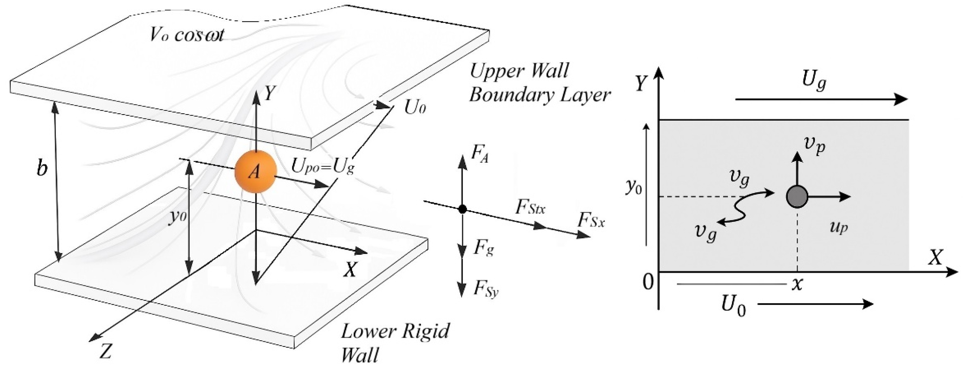
Figure 2.
Conceptual representation of the impulsive forcing term ∑Ikδ(t−tk) acting on particle velocity components in the analytical model.
Figure 2.
Conceptual representation of the impulsive forcing term ∑Ikδ(t−tk) acting on particle velocity components in the analytical model.
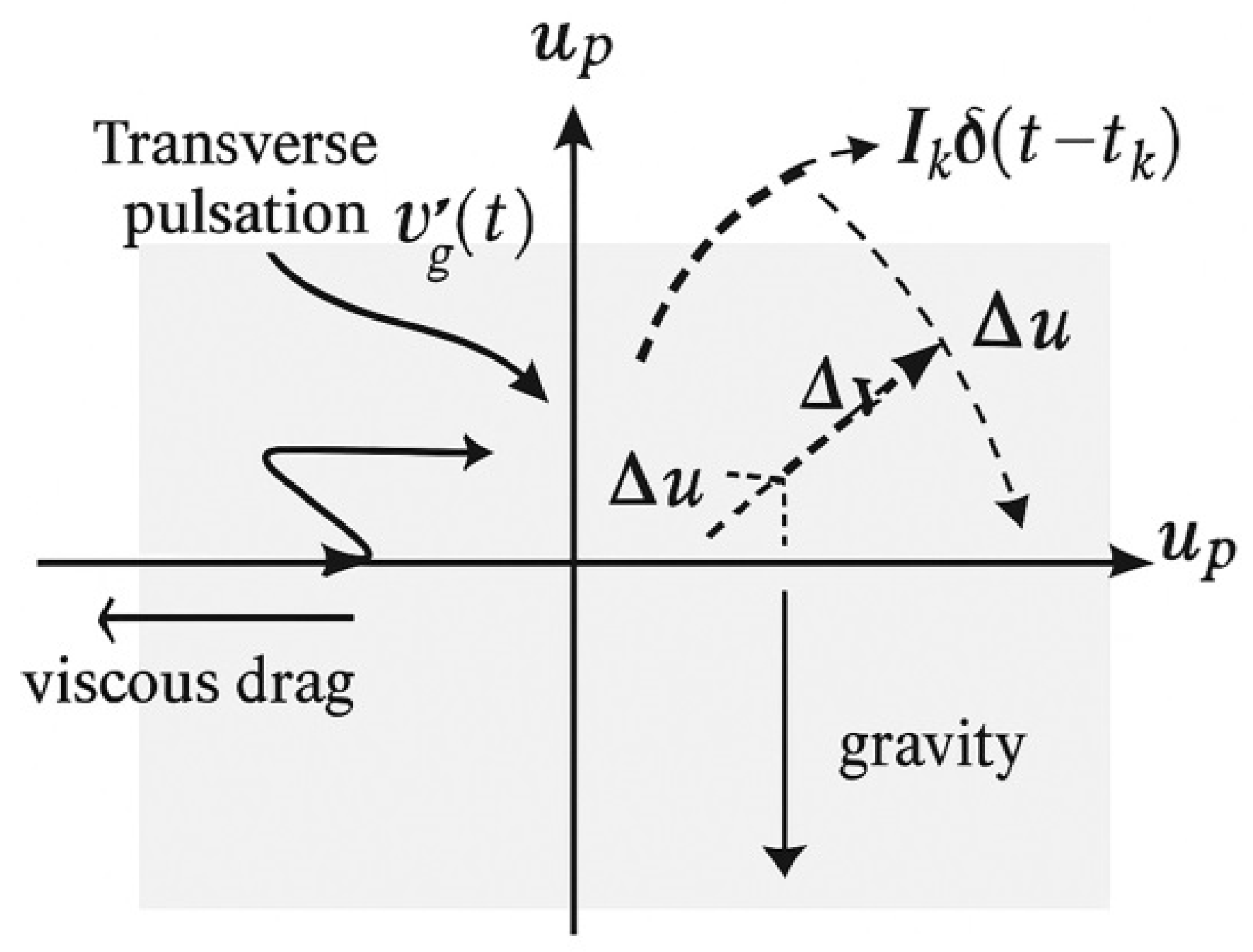
Figure 3.
Schematic illustration of the operator-based description of particle motion, highlighting the mapping between initial conditions, external forcing, and particle response via the resolvent operator (sI−M)−1.
Figure 3.
Schematic illustration of the operator-based description of particle motion, highlighting the mapping between initial conditions, external forcing, and particle response via the resolvent operator (sI−M)−1.
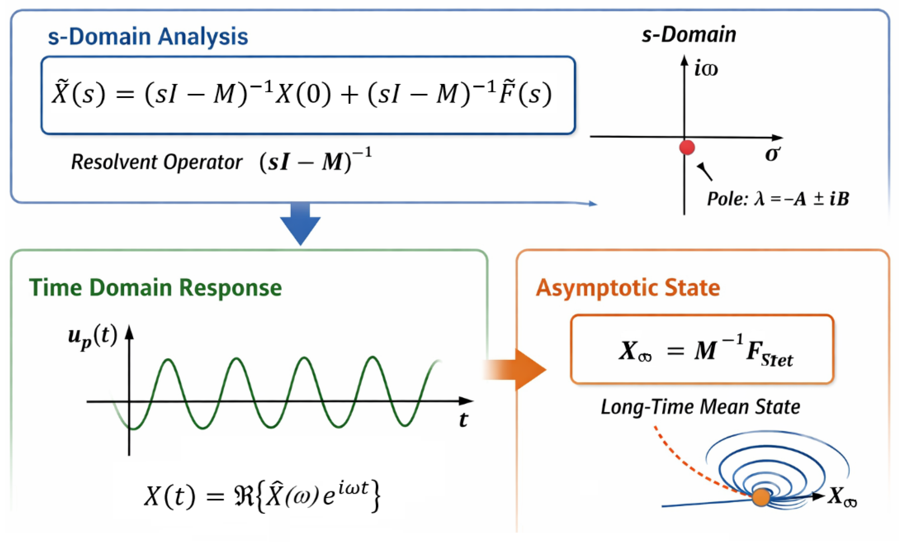
Figure 4.
Transverse particle velocity vp(t) for light and heavy particles.
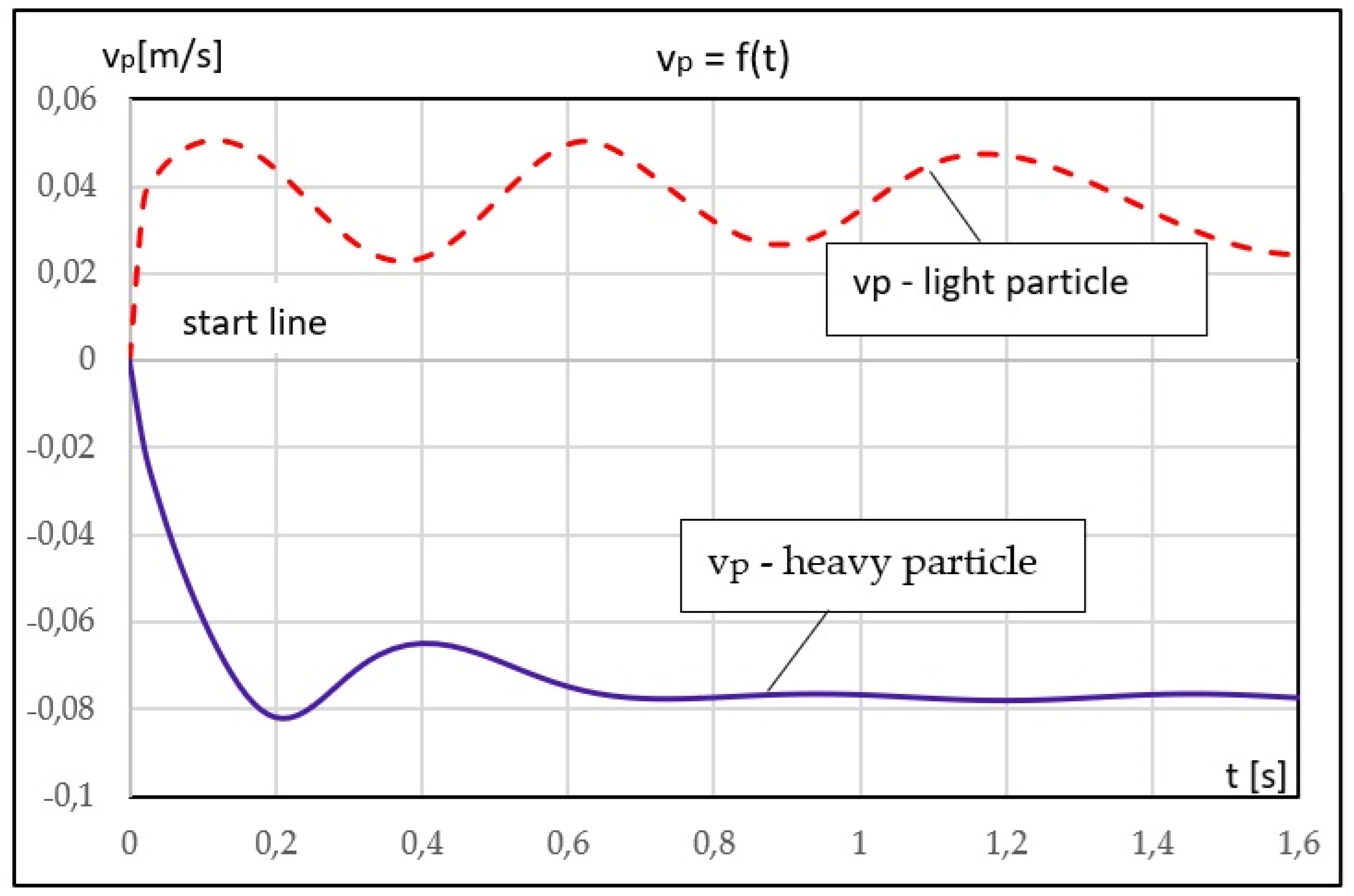
Figure 5.
Transverse particle displacement y(t) for light and heavy particles.
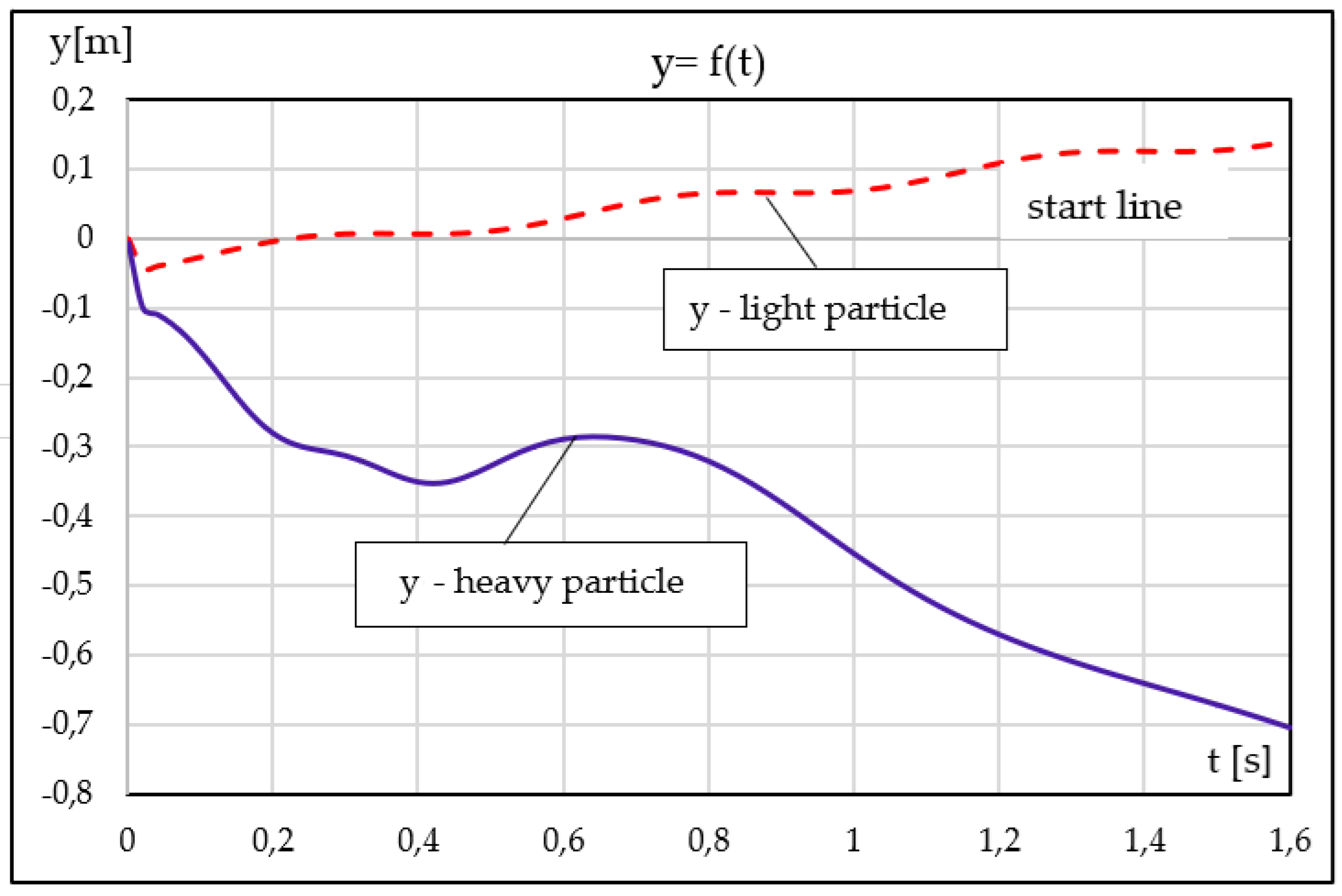
Figure 6.
Longitudinal particle velocity uₚ(t) for light and heavy particles.
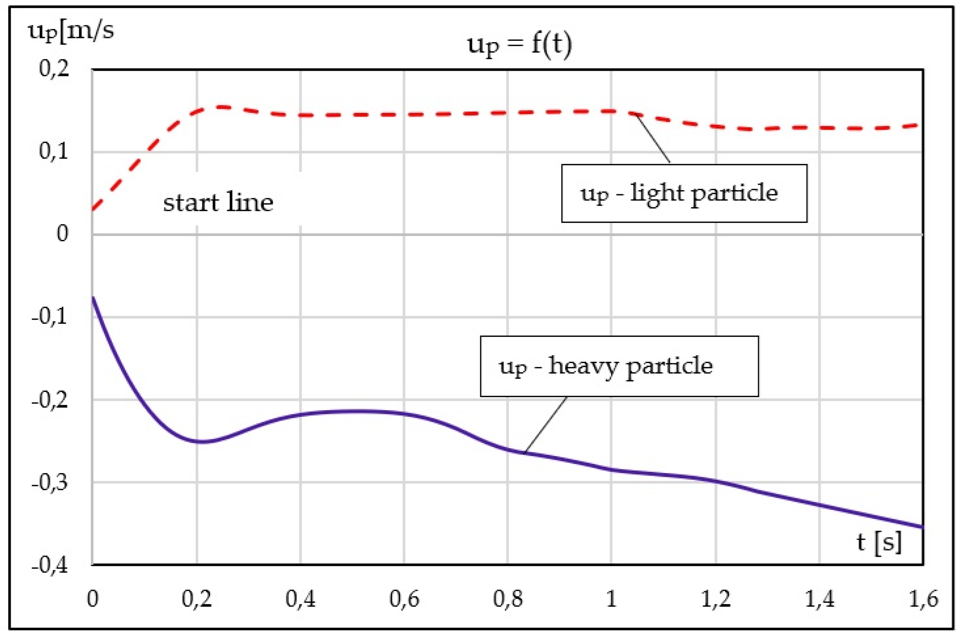
Figure 7.
Longitudinal particle displacement x(t) for light and heavy particles.
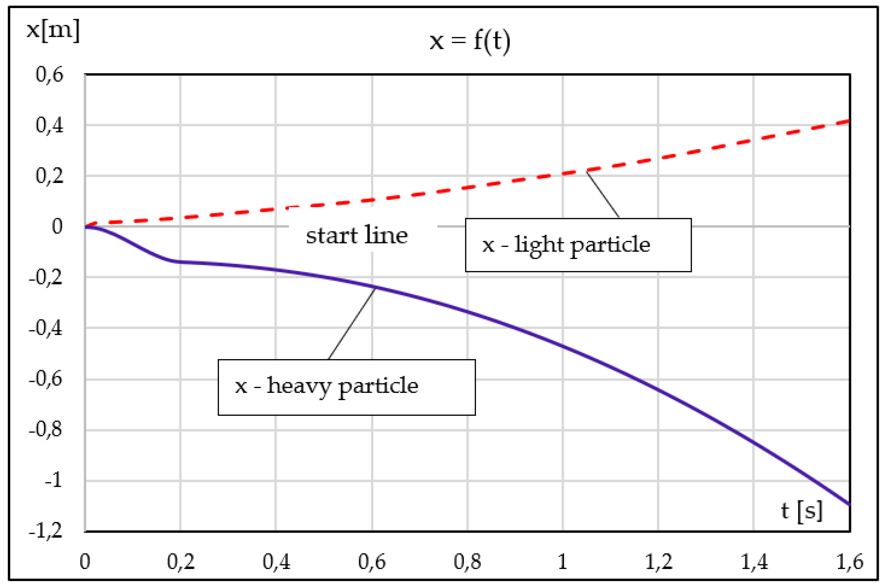
Figure 8.
Impulsive phase–space dynamics of light and heavy particles.
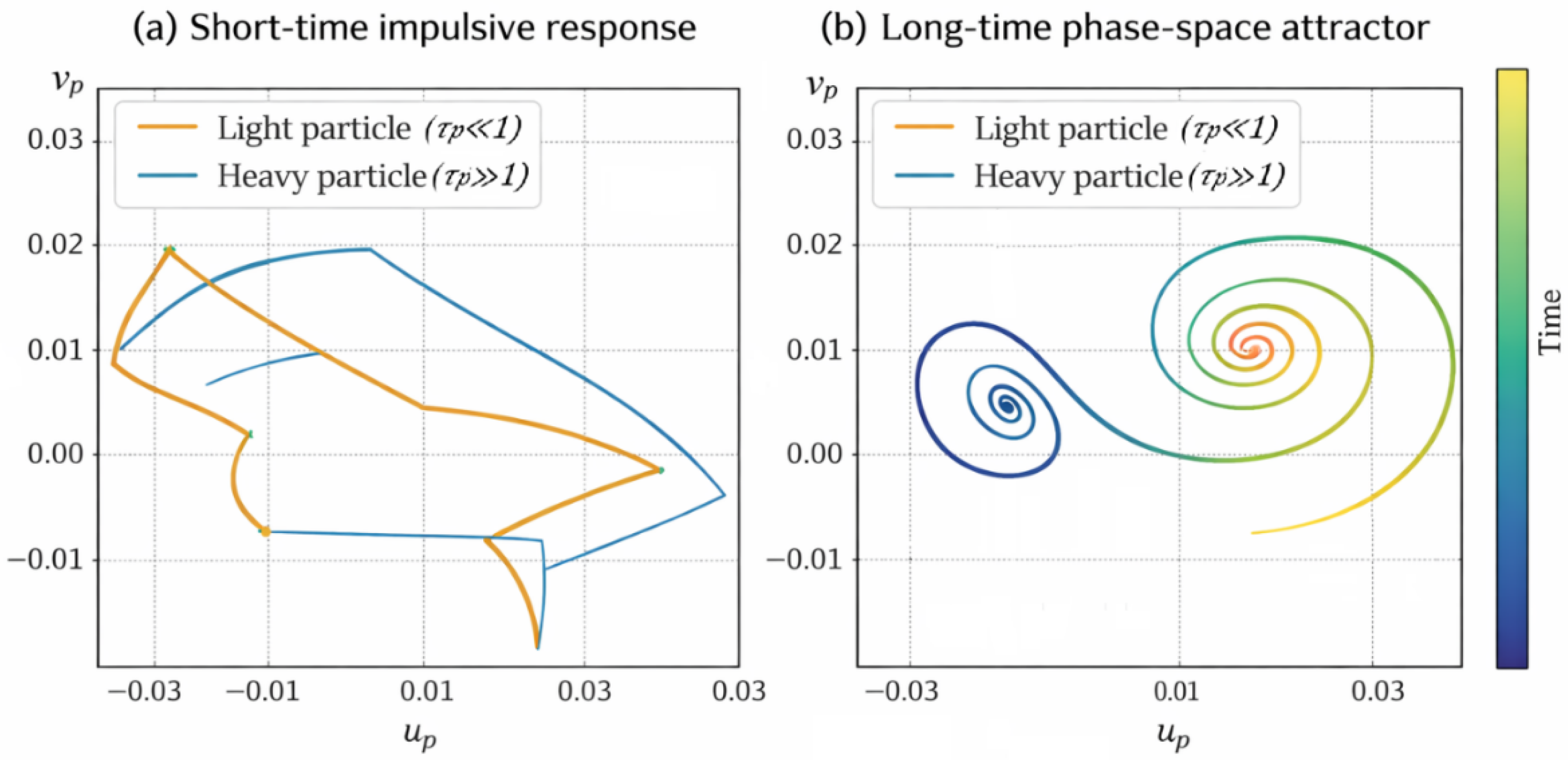
Figure 9.
Phase–space trajectories obtained from the matrix formulation under harmonic forcing.
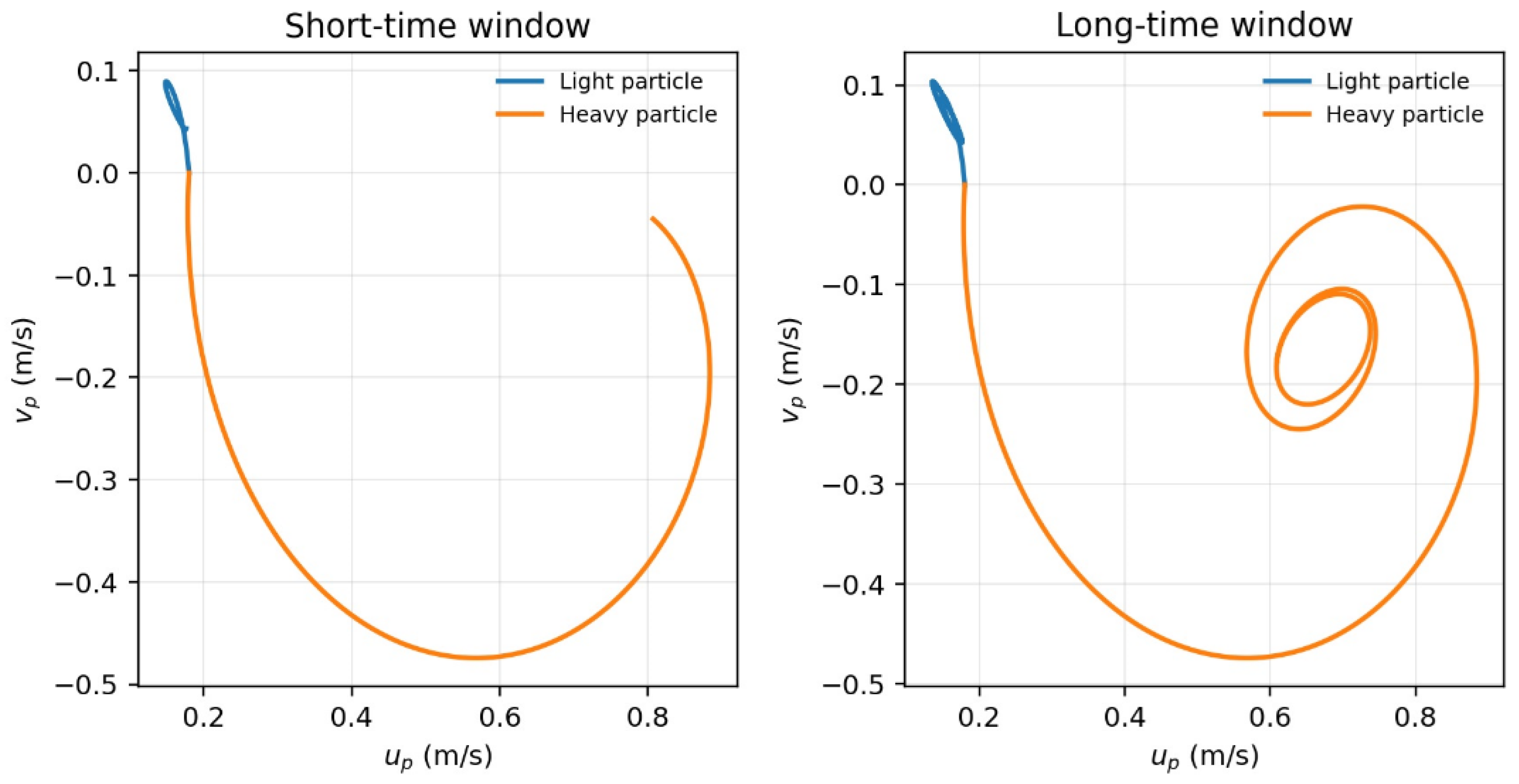
Figure 10.
Resonance amplitude under harmonic forcing.
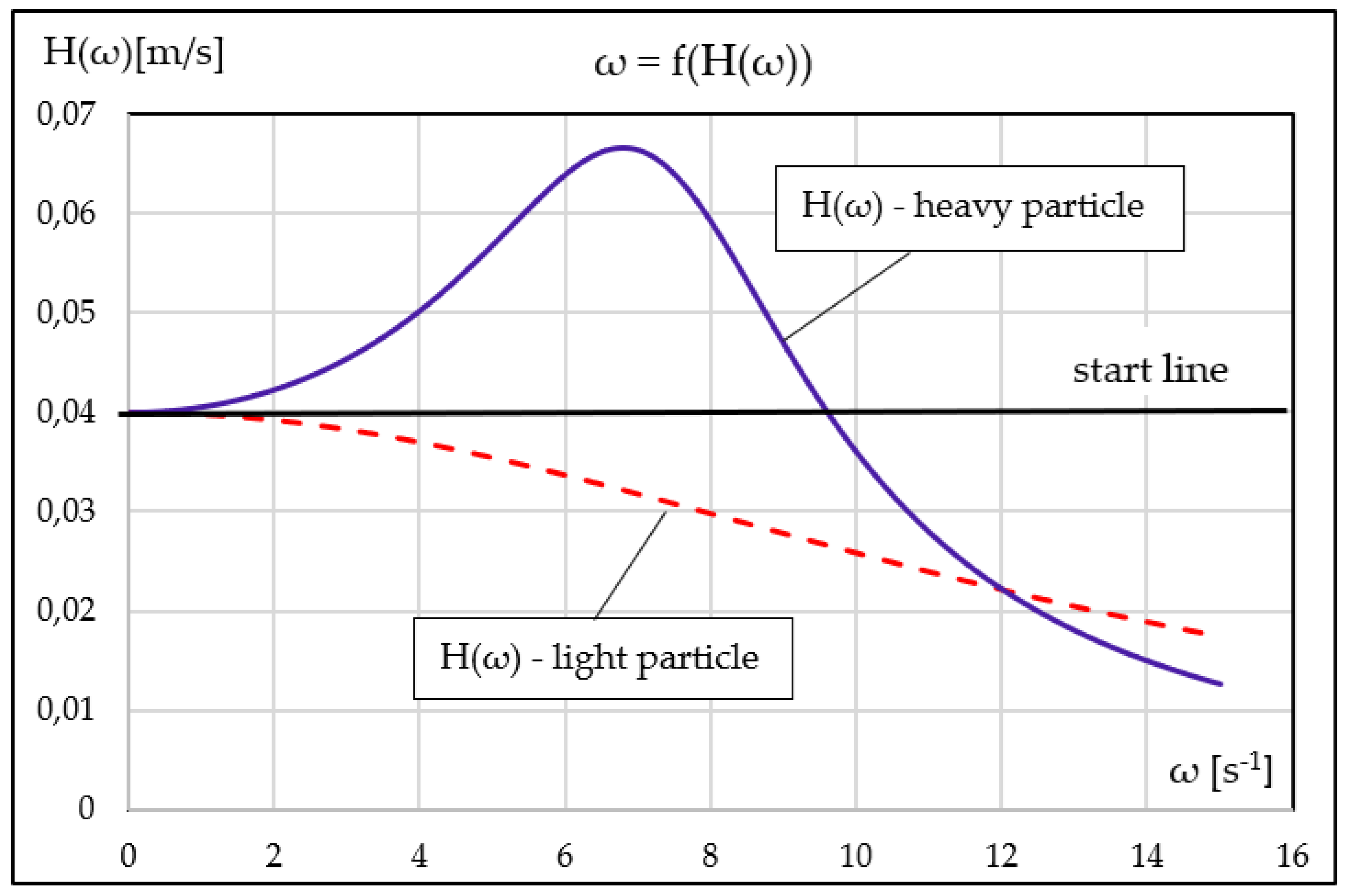
Figure 11.
Phase–space trajectories (up,vp) of light and heavy particles under multi-harmonic transverse forcing.
Figure 11.
Phase–space trajectories (up,vp) of light and heavy particles under multi-harmonic transverse forcing.
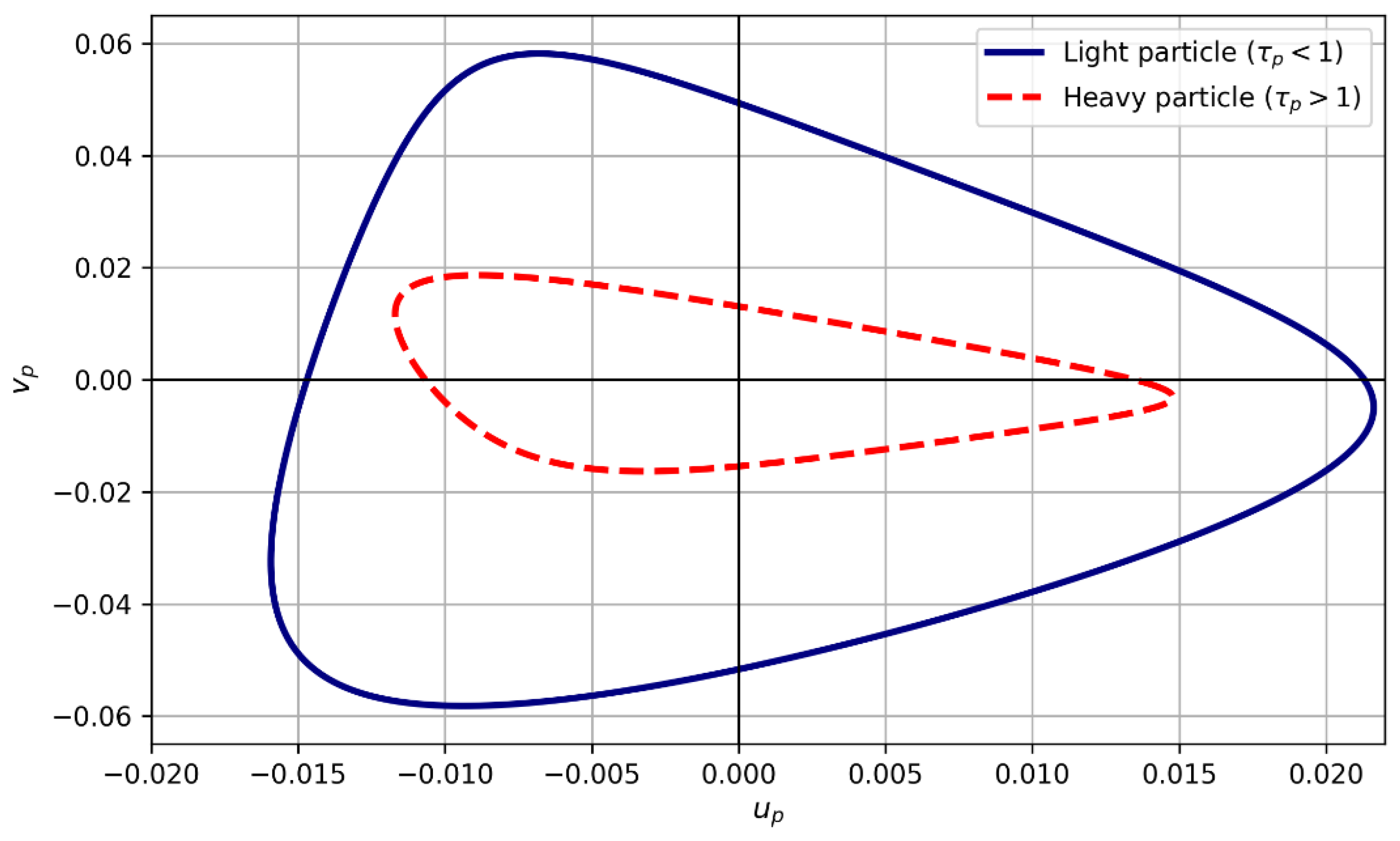
Figure 12.
Asymptotic phase–space trajectories of particles with different inertial response.
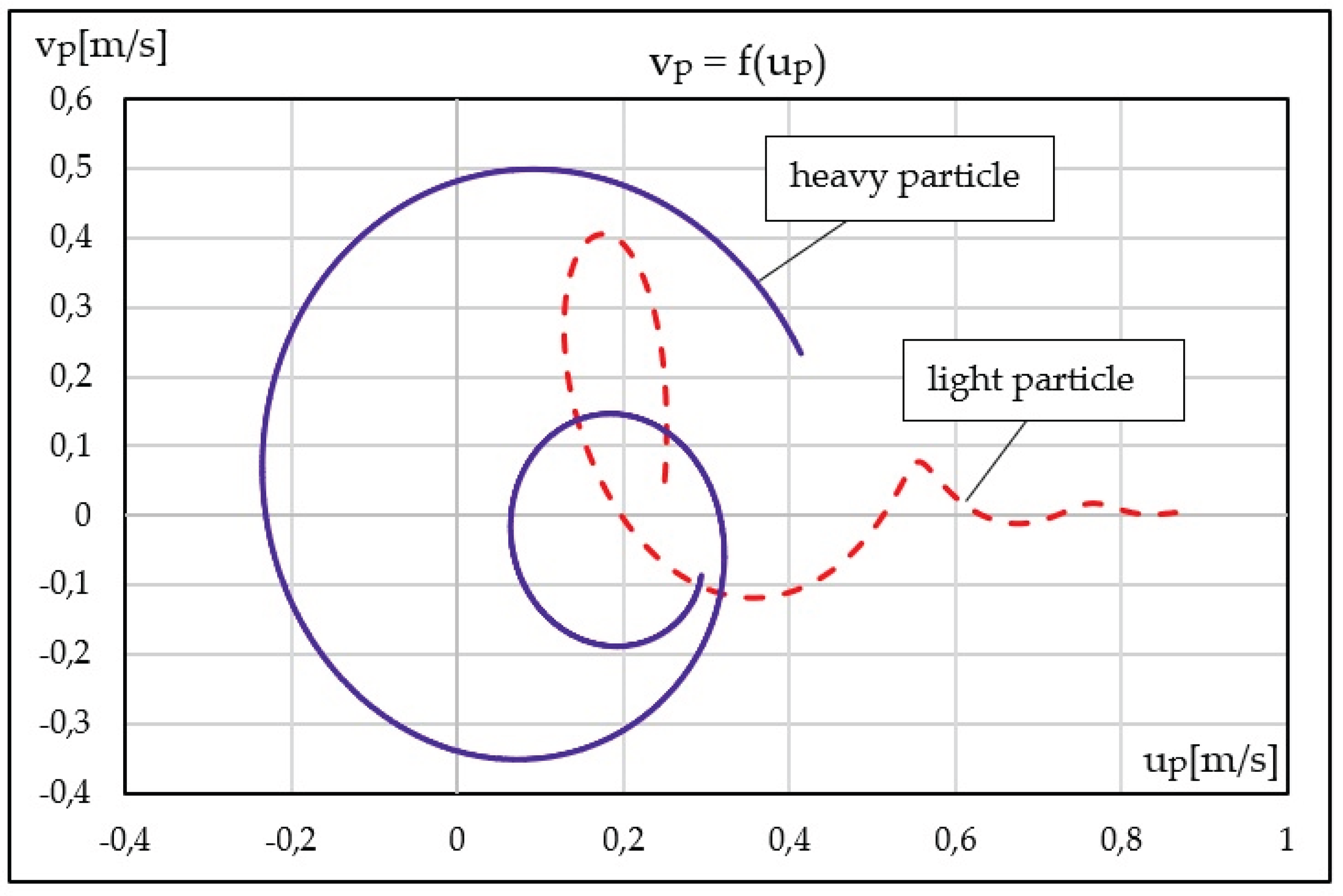

Table 1.
Fluid and boundary-layer parameters.
| Parameter | Symbol | Value | Unit |
| Fluid type | - | Water (T ≈ 20 °C) | - |
| Kinematic viscosity | ν | 1.0x10⁻⁶ | m2/s |
| Fluid density | ρf | 998 | kg/m3 |
| Shear rate | γ | 80 | s-1 |
| Outer-stream velocity | U∞ | 0.392 | m/s |
| Boundary-layer thickness | δ | 0.064 | m |
| Wall shear rate | γω | 6.142 | s-1 |
| Pulsation frequency | ω | 1.93 | rad/s |
Table 2.
Particle parameters.
| Parameter | Symbol | Light particle | Heavy particle | Unit |
| Density | ρp | 1050 | 3000 | kg/m3 |
| Relaxation time | τp | 0.012 | 0.18 | s |
| Density ratio | εp | 1.05 | 3.00 | - |
| Particle diameter | dp | 0.00045 | 0.00104 | m |
| Initial position | (x0,y0) | (0,0) | (0,0) | m |
| Initial velocity | (up,vp) | (Ug(y0),0) | (Ug(y0),0) | m/s |
Table 3.
Numerical configuration.
| Parameter | Value | Unit |
| Time step Δt | 1.0x10⁻³ | s |
| Total duration | 1.6 | s |
| Method | RK4 | - |
| Output sampling | 0.02 | s |
Disclaimer/Publisher’s Note: The statements, opinions and data contained in all publications are solely those of the individual author(s) and contributor(s) and not of MDPI and/or the editor(s). MDPI and/or the editor(s) disclaim responsibility for any injury to people or property resulting from any ideas, methods, instructions or products referred to in the content. |
© 2026 by the authors. Licensee MDPI, Basel, Switzerland. This article is an open access article distributed under the terms and conditions of the Creative Commons Attribution (CC BY) license (http://creativecommons.org/licenses/by/4.0/).
Copyright: This open access article is published under a Creative Commons CC BY 4.0 license, which permit the free download, distribution, and reuse, provided that the author and preprint are cited in any reuse.


