Submitted:
04 January 2026
Posted:
06 January 2026
You are already at the latest version
Abstract
This study presents a comprehensive thermal analysis, design, and optimization framework for electrothermal heating systems integrated into composite wing structures. Thermal behavior is first investigated using finite volume simulations conducted with a commercial solver. An in-house thermal solver is then developed based on the governing heat transfer equations and a second-order finite difference discretization scheme. The in-house solver is validated against the commercial solver, showing a maximum deviation less than 1%. The validated solver is subsequently coupled with a genetic algorithm to perform multi-objective optimization of the electrothermal heating system. A novel correlation for the convection heat transfer coefficient over airfoil surfaces is developed based on extensive turbulent flow simulations and genetic algorithm. The developed correlation equation has significantly lower percent relative error (from 34% to 6%) compared to flat plate correlations. The developed convection coefficient is incorporated into the optimization process. Key design variables including heat generation intensity, heater strip dimensions, and the thermal conductivity of composite and surface protection materials are included in the optimization process. An original objective function is formulated to simultaneously minimize electrical power consumption, prevent ice formation on the external surface, and limit internal temperatures to safe operating ranges for composite materials. The optimized design is evaluated under both spatially varying and constant convection heat transfer coefficients to assess the impact of convection modeling assumptions. The proposed methodology provides a unified and extensible framework for the optimal design of electrothermal ice protection systems and can be readily extended to three-dimensional composite wing configurations.
Keywords:
composite structures
; thermal analysis in composites
; genetic algorithm based optimization
; electrothermal heating in wings
1. Introduction
Aircraft icing represents a major threat to flight safety, as ice accretion degrades aerodynamic performance by increasing drag, reducing lift, and potentially inducing premature stall [1]. Extensive studies on icing physics and operational impacts have demonstrated that ice accumulation on wing leading edges is particularly critical when aircraft operate in supercooled droplet conditions [1,2]. Consequently, effective ice protection systems are essential for maintaining aerodynamic efficiency and ensuring safe flight operations.
In modern aircraft design, composite materials are increasingly employed in wing structures due to their high specific stiffness, favorable elastic properties, and reduced weight compared to metallic counterparts. However, the relatively low thermal conductivity and narrow allowable operating temperature range of composite materials introduce significant challenges for de-icing and anti-icing applications. Conventional ice protection systems based on engine bleed air, while effective for metallic wings, are increasingly incompatible with composite airframes because of high energy losses, added system complexity, and integration difficulties [3]. As a result, the development of efficient active thermal management systems for composite wings has become a critical research area, with particular emphasis on flight safety and energy efficiency. To improve structural integration, heating elements are commonly embedded within fiber-reinforced polymer (FRP) laminates.
In recent years, a wide range of materials have been investigated as heating elements for electrothermal ice protection systems, including graphene-based materials [4,5] carbon fibers [6,7], carbon nanotubes (CNTs) [8,9,10,11,12] and 3D printed heater materials [13,14]. While these studies have demonstrated the feasibility of electrothermal heating in composite structures, the majority focus on material selection or proof-of-concept implementations rather than systematic design optimization.
Several investigations have explored electrothermal heating configurations in composite wing structures. Carbon fiber reinforced plastic (CFRP) wings incorporating electrothermal heating systems have been studied using a limited number of heater configurations, largely based on trial-and-error approaches [15]. Similarly, experimental studies on glass fiber reinforced polymer (GFRP) composites have examined the effects of heater placement without performing formal optimization of parameters such as heater size, location, power consumption, or temperature uniformity [16]. Discrete constantan heating elements embedded in composite airfoils have been tested under dry and icing conditions [17], while subsequent work highlighted potential structural concerns such as delamination [18]. However, these studies did not include optimization of heater positioning, power input, or thermal performance metrics.
Additional heat transfer investigations have examined carbon composite structures with copper heating plates under varying heat generation levels [19]. Although the study demonstrated viable heating performance, it did not propose a systematic design methodology or optimization framework.
Only a limited number of studies have attempted optimization of electrothermal heating systems. In these works, optimization objectives were typically restricted to either minimizing power consumption [20] or reducing total de-icing time [21,22]. While valuable, such approaches do not account for the multi-objective nature of electrothermal ice protection system design, which must simultaneously address thermal uniformity, structural and aerodynamic safety, power efficiency, heater sizing and placement, and material constraints.
Based on a critical review of the existing literature, two major research gaps are identified. First, there is a lack of unified, multi-objective optimization frameworks capable of improving electrothermal heating system design from multiple, interdependent perspectives. Existing studies rarely integrate thermal uniformity, energy consumption, heater geometry and positioning, and material limitations into a single objective formulation. Second, numerical studies commonly oversimplify external convective heat transfer effects by employing constant convection coefficients derived from one-dimensional correlations, thereby neglecting the spatially varying nature of airflow over airfoil surfaces.
To address these gaps, a novel finite difference based solver is developed and validated as part of the study. The developed solver removes restrictions on the possible boundary conditions such as smoothly varying convection heat transfer coefficient and tackles difficulties associated with coupling the solver with the desired optimization code in an efficient manner. The developed solver is utilized in the optimization studies.
The present study proposes a novel unified optimization approach for electrothermal heating systems in composite wing structures. It targets both minimization of power consumption while keeping the temperatures at an acceptable range. The minimization of the electrical power consumption is very important since energy consumption levels as high as 100 kW are observed in aircraft [2].
While previous experimental studies generally utilize the trial and error approach for the determination of suitable range of electrical power input [7], the current study directly optimizes the heat input that leads to a balanced temperature distribution across the structure. Instead of a constant convection heat transfer coefficient,developed locally varying heat transfer coefficient is utilized in the numerical analyses and optimization runs.
While most of the existing studies embed buckypaper into glass fiber reinforced plastic structure, the utilization of buckypaper inside the composite along with a surface coating material that mitigates risks associated with the fragility of the buckypaper [23] which at the same time improves thermal behaviour is not thoroughly analyzed in the literature. The current study fills this research gap by numerically simulating such a configuration, which indicates the importance of high conductivity for the surface coating material.
Another novelty area of the study is about the introduction of the heater thickness as an optimization variable. While the thickness of the heater is generally taken as constant in the existing studies [8,22,24,25] the optimum thickness of the heater is studied as part of one of the optimization studies contained in this manuscript.
The objective function simultaneously minimizes power consumption while constraining excessive temperatures that may lead to material degradation or structural failure, and ensuring a safe and uniform temperature distribution within the composite domain.
The study also provides some important steps for the introduction of lamina ply angles as optimization variables for the electrothermal system optimization on the composite stuctures. These points are generally not studied in the existing optimization studies towards electrothermal heating systems due to associated high computational costs.
Furthermore, this study introduces a new correlation for the convective heat transfer coefficient over airfoil surfaces, developed using genetic algorithm over a newly formed database of 108 RANS simulations. This approach eliminates the conventional assumption of constant convection coefficients and captures local variations in heat transfer behavior. To the authors’ knowledge, this is the first study to employ an evolutionary algorithm to derive convection heat transfer correlations for electrothermal anti-icing applications on airfoils.
2. Method
In this study, a multi-stage numerical methodology is employed to analyze and optimize electrothermal heating systems for composite wing structures. Initially, computational fluid dynamics (CFD) simulations are performed using a commercial flow solver to investigate convective heat transfer characteristics over different geometries. Both airfoil sections and two-dimensional flat plates are analyzed, with the latter subjected to convective conditions representative of those observed in airfoil flows.
Subsequently, a dedicated thermal solver is developed with the primary objective of enabling efficient and flexible integration with optimization algorithms. The solver is formulated based on the governing heat transfer equations and validated against results obtained from the commercial solver. In the commercial simulations, the finite volume method is employed, and diffusive terms in the heat conduction equation are discretized using a second-order central differencing scheme with a node-based approach.
In the final stage, optimization studies are conducted. First, a correlation equation for the convective heat transfer coefficient is developed using data obtained from CFD simulations. The validated in-house thermal solver is then coupled with a genetic algorithm to determine optimal electrothermal heating configurations. Once the optimal design is obtained, its thermal performance is evaluated under both constant and spatially varying convective heat transfer coefficients. The resulting temperature distributions and power requirements are compared and discussed. A schematic overview of the complete numerical and optimization workflow is presented in Figure 1.
The numerical study presented in Section 4.1 is linked with the optimization study presented in Section 5.1. The numerical study presented in Section 4.2 and Section 4.3 are related to optimization studies presented in Section 5.2 and Section 5.3. The study flows from 2 branches to achieve its goals. This is schematically explained by Figure 1.
3. Mathematical Equtions of Interest
In GFRP, specific heat capacity values vary slightly with fiber volume ratio [26]. Thermal conductivity in the longitudinal direction can be represented by the following simple law of mixtures;
Heat conduction coefficient in the transverse direction can be found with the following model [27];
In equation (2), subscript 2 corresponds to fiber, subscript m corresponds to resin. Volumetric ratio of fiber is given by the vf term.
For ply fiber orientations other than 00, effective conductivities can be found with the following formula:
where, Eqn. (1) and Eqn. (2) can be used to obtain kxx and kyy, respectively.
If the effect of heat generation is included, unsteady heat equation can be represented as [25];
Continuity equation is given by;
X momentum equation is given by;
Y momentum equation is given by;
With the inclusion of flow related convective terms, unsteady energy (temperature) equation is given by;
Note that unsteady heat conduction equation given by Equation (5) is solved in solid domain, while unsteady energy equation given by Equation (9) is solved in fluid domain.
In Equations (7-9), su, sv, sT terms represent source term. The coefficient is effective viscosity which includes the effects of molecular and turbulent viscosities. Turbulent viscosity is then calculated with realizable realizable k–ε model. Further information is given in Section 4.1.
Equations (6-9) are solved for the flow over airfoil analyses provided in Section 4.1 which provides the basis for the optimization study given in Section 5.1. Equations (1-5) are solved in numerical analyses provided in Section 4.2 and Section 4.3; and in optimization studies (5.2), (5.3) for each population member of the genetic algorithm.
If the coordinate system is curvilinear and orthogonal, the heat equation can be represented by [28];
where the orthogonal scale factors are given by
For the airfoil,
is utilized.
h1 = 1 + κ (s)*n, h2=1
κ(s), h1, h2 terms represent local curvature, tangential scale factor and normal scale factor, respectively. Since we evaluate heat transfer at the airfoil surface where the distance is nearly zero, the term becomes approximately 1.
Substituting these into the general formula;
Eq. (13) is utilized in the upcoming section when flat plate and curved airfoil shells are compared.
4. Numerical Analysis
4.1. CFD Analyses over Airfoil for Obtaining Convection Heat Transfer Coefficient
To determine the convective heat transfer coefficient, Reynolds-averaged Navier–Stokes (RANS) simulations coupled with the energy equation are performed. Steady, incompressible two-dimensional flow over 3 different airfoils is considered at zero angle of attack. A total of 108 Reynolds Averaged Navier Stokes (RANS) simulations are performed. A structured C-type mesh is employed, as shown in Figure 2. The computational domain extends from −11.5 m to 21 m in the streamwise (x) direction and from −12.5 m to 12.5 m in the transverse (y) direction. The airfoil chord length is 1 m.
The simulations are conducted using a pressure-based solver with the SIMPLE algorithm for pressure–velocity coupling. Convective fluxes for the momentum, energy, turbulent kinetic energy (k), and dissipation rate (ε) equations are discretized using second order upwind scheme. Diffusive fluxes for the momentum, energy, turbulent kinetic energy (k), and dissipation rate (ε) equations are computed with second order central difference scheme. Convergence is assessed using residual thresholds of 10−6 for pressure, velocity, temperature, and continuity, and 10−5 for the turbulence equations. Under-relaxation factors of 0.3 for pressure, 0.7 for momentum, and 0.8 for k and ε are applied to ensure numerical stability.
The realizable k–ε turbulence model with the Menter–Lechner wall function is employed. 36 different Reynolds numbers are investigated over 3 different airfoils of (NACA 0012, NACA 0015, NACA 0018; NACA standing for National Advisory Committee for Aeronautics) by varying the inlet velocity between 15 m/s-50 m/s. The velocity range is selected so as to simulate the working range of small-medium UAVs[29]. The angle of attack effects are not included in this study, as it makes the upper and lower sides of the airfoil behave differently, adding further complexity to the analysis.
Air properties are assumed constant, with density set to 1 kg/m3, dynamic viscosity to 1.6 × 10⁻⁵ Pa·s, and thermal conductivity to 0.0242 W/m·K. The corresponding Reynolds numbers based on chord length are between 9.37 × 10⁵ -3.12 × 10⁶, respectively.
The resulting convective heat transfer coefficient distributions along the NACA 0012 airfoil surface are shown in Figure 3. As observed, the local heat transfer coefficient varies significantly along the chord, reaching a maximum near the leading edge at approximately 0.1*chord length and decreasing toward the trailing edge. Additionally, the magnitude of the heat transfer coefficient increases with increasing Reynolds number. These trends are subsequently incorporated into the electrothermal heating optimization framework through the proposed convection correlation to improve heating efficiency and thermal uniformity.
For NACA 0015 and NACA 0018 airfoils, h distribution along the chord length is given by Figure 6 and Figure 7, respectively. They are very similar to the NACA 0012.
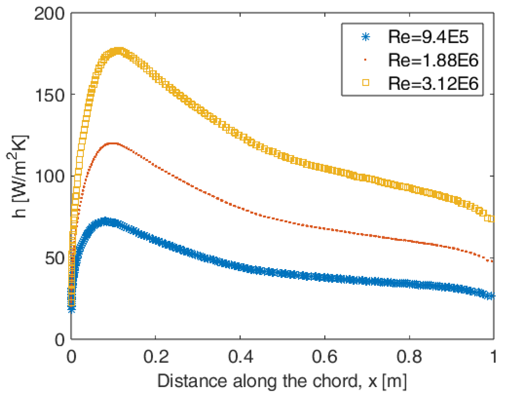
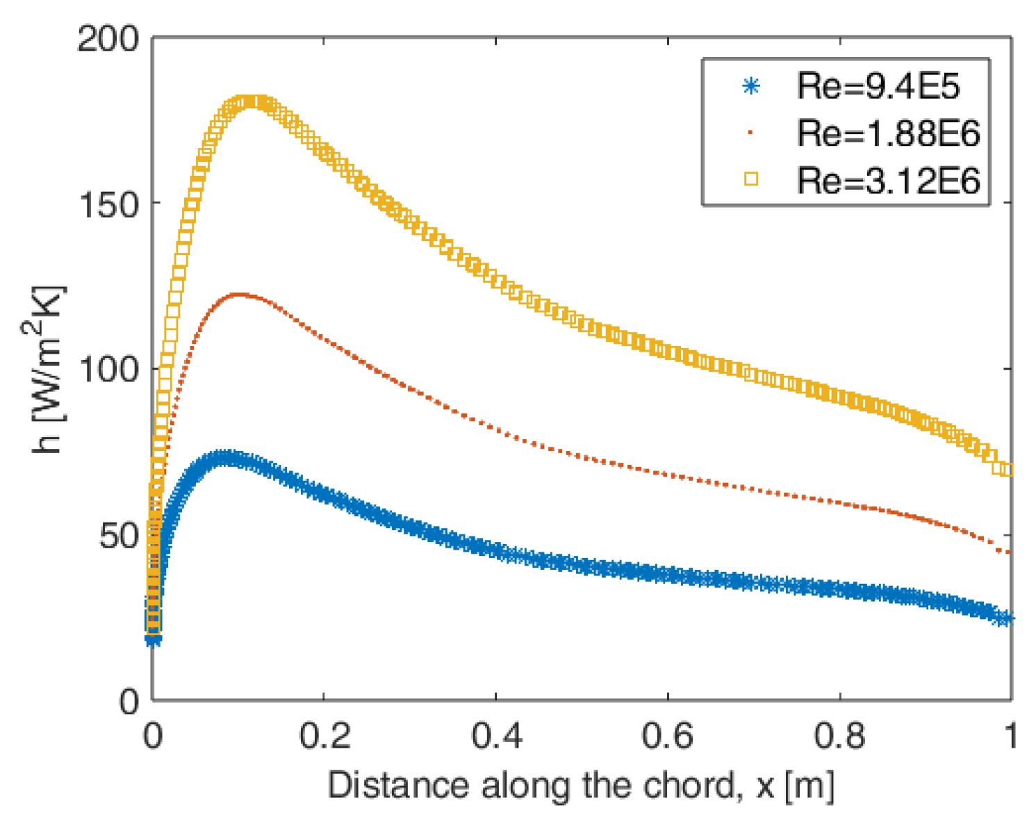
Figure 4.
Chordwise variation of the convective heat transfer coefficient (h) for different Reynolds numbers along the NACA 0015 airfoil surface.
Figure 4.
Chordwise variation of the convective heat transfer coefficient (h) for different Reynolds numbers along the NACA 0015 airfoil surface.
Figure 5.
Chordwise variation of the convective heat transfer coefficient (h) for different Reynolds numbers along the NACA 0018 airfoil surface.
Figure 5.
Chordwise variation of the convective heat transfer coefficient (h) for different Reynolds numbers along the NACA 0018 airfoil surface.
4.2. Plate Thermal Analyses
Heat generation within the composite domain is assumed to be spatially uniform. This assumption is consistent with electrothermal heating achieved using nickel-coated carbon composite laminates [30]. The top and bottom surfaces of the composite plate are subjected to convective heat transfer, while the left and right boundaries are prescribed as isothermal surfaces. A constant convection heat transfer coefficient of 50 W/m2·K is applied on the top and bottom surfaces, with a freestream temperature of 253 K. The left and right boundaries are maintained at a fixed temperature of 273 K.
Volumetric heat generation rates of 2.0 × 10⁴, 2.5 × 10⁴, and 3.0 × 10⁴ W/m3 are considered in the simulations. The composite material density is taken as 1.8 × 10³ kg/m3, and the specific heat capacity is assumed to be 1.0 × 10³ J/(kg·K). Two cases are investigated: an isotropic case (k = 0.5 W/m·K) and an orthotropic case (kₓ = 0.8 W/m·K, ky = 0.5 W/m·K), allowing assessment of non-isotropic heat conduction effects.
The composite plate dimensions are 1.0 m × 0.1 m. A grid independence study is performed by progressively refining the mesh until the variation in mid-plane temperature is less than 1%. Uniform grids of 20 × 20, 40 × 40, 80 × 80, and 100 × 100 cells are evaluated. Based on this study, a mesh consisting of 100 divisions in both the x and y directions is adopted for all subsequent simulations.
To accurately capture steep thermal gradients near the convective boundaries, grid clustering is applied in the wall-normal (y) direction. The ratio of the maximum to minimum cell edge length in the y direction is defined as;
The minimum cell edge length in the y direction closest to the wall is just 0.2 mm.
For the cases where thermal gradients are higher and non-isotropic materials are used, the advantage of mesh clustering is more pronounced. Figure 6 illustrates the grid structure.
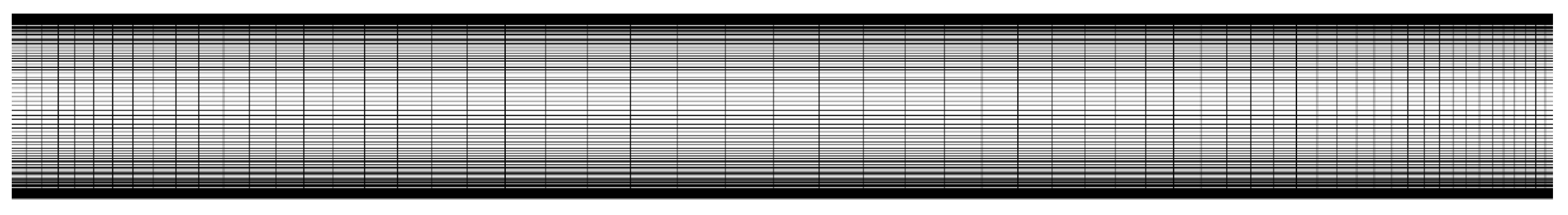
Figure 6.
Computational grid structure of the composite slab used in the thermal validation simulations.
Figure 6.
Computational grid structure of the composite slab used in the thermal validation simulations.
Quadrilateral elements are employed in the computational grid, as they generally provide improved numerical accuracy for heat conduction problems. Node clustering is applied near the external surfaces to accurately capture steep thermal gradients in regions subjected to convective heat transfer.
Figure 7 presents the mid-plane temperature distributions for various volumetric heat generation rates (20–30 kW/m3) and for both isotropic and orthotropic thermal conductivity cases. The results indicate that, for a given heat generation level, the composite structure exhibits lower temperatures when orthotropic thermal conductivity is considered compared to the isotropic assumption.
This behavior highlights the importance of accurately representing anisotropic heat conduction in composite materials. Modeling the composite as isotropic leads to higher predicted temperatures and may therefore result in non-conservative assessments of thermal performance and structural safety. In contrast, the orthotropic model captures directional heat transfer effects more realistically, providing a more reliable basis for electrothermal heating system design.
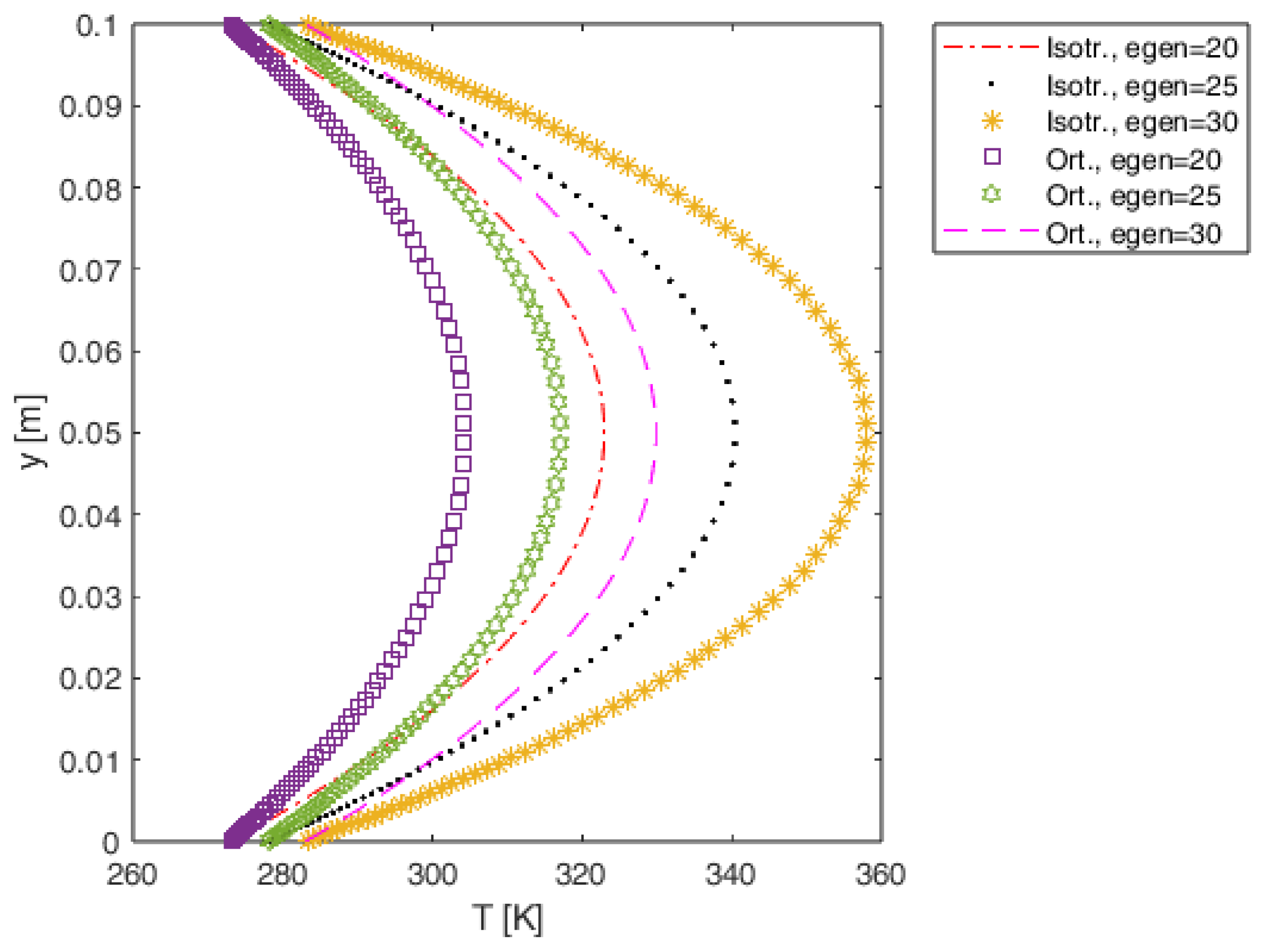
Figure 7.
Mid-plane temperature distributions for different volumetric heat generation rates (20–30 kW/m3) and for isotropic and orthotropic thermal conductivity cases.
Figure 7.
Mid-plane temperature distributions for different volumetric heat generation rates (20–30 kW/m3) and for isotropic and orthotropic thermal conductivity cases.
4.3. In-House Solver
An unsteady finite-difference-based 2D thermal solver is utilized to enable flexible and efficient conduct of optimization studies [31]. Spatial discretization of the heat conduction equation is performed using a second-order central differencing scheme, while temporal integration is carried out using a first-order explicit Euler method. The time step is selected to maintain the stability of the scheme, corresponding to a sufficiently small time increment that minimizes truncation errors associated with first-order time integration. Mesh Fourier number associated with the stability of the explicit scheme is given by [32]
Thermal diffusivity terms are given by
In this study, a maximum mesh Fourier number value of 0.1 is used to ensure stability and improve numerical accuracy. Various boundary conditions (isothermal, insulated, convective) are implemented in the discretized governing equations. The thermal solver is implemented in MATLAB R2024a. Convergence is evaluated using a percent relative error criterion, and iterations are continued until the error falls below 10−8.
The results obtained from the in-house thermal solver are validated against temperature predictions from the ANSYS Fluent solver for cases involving homogeneous volumetric heat generation.
In the first validation study, a convection heat transfer coefficient of 50 W/m2·K is applied at the top and bottom surfaces, with a freestream temperature of 253 K. The left and right boundaries are prescribed as isothermal surfaces at 273 K. The specific heat capacity of the composite material is taken as 1.0 kJ/(kg·K). The plate dimensions and thermal conductivity values are consistent with those used in the corresponding commercial finite volume simulations. A grid independence study is performed, and the mesh is refined till the change in the temperature results drop below 1%. The final computational mesh consists of uniformly spaced nodes, with a total of approximately 4.0 × 10⁴ nodes for the 2D problem. The comparison of Fluent and custom solver results indicates a percent relative error of less than 1%, demonstrating good agreement between the two approaches. Figure 8 illustrates the good correlation between Fluent and novel thermal solver results.
A mesh independence study is also made for the case. Results are illustrated in Figure 9, showing good convergence behaviour as the mesh is refined.
In the second validation study, left and right boundaries are insulated, while the top and bottom boundary is subjected to convection (h=50 W/m2.K, Tinf=253 K). Heat is uniformly generated inside the plate. Comparisons are made between Fluent and novel thermal solver results. The results are shown in Figure 10 which indicate the high accuracy and robustness of the solver.
The effect of the mesh Fourier number is investigated. The transient thermal solver is propagated for 360 s, with a mesh Fourier number of 0.1, and 0.01 for the orthotropic plate. A heat generation rate of 20e3 W/m3 is applied inside the plate, and the upper and lower plates are subjected to a constant convection heat transfer, h=50 W/m.K, and Tinf=253 K. 40 000 cells are utilized in the mesh as before. The results are almost identical between the cases as shown by Figure 11 and Figure 12. Mean relative error obtained by comparing the two cases with different mesh Fourier numbers is 8.2e-6.
Another validation study is performed by comparing the 2D steady state analytical solution with the numerical solution. The top edge of the 2D plate is at 320 K, while the remaining edges are at 220 K. The domain is 1x1 m in size. The number of cells in the domain is 40 000. The analytical solution at the steady state is given by [33];
The series index is taken up to n=200 for the calculation of the analytical solution. The results of the analytical and numerical analyses are given by Figure 13 and Figure 14, respectively. The results are again very similar, with mean relative error of 6.7e-4.
An additional numerical validation study was performed with piecewise constant convection heat transfer coefficient introduced into commercial and in-house solvers. A 2D plate with dimensions 1 m x 0.1 m is used. A constant heat generation rate of 20x103 (W/m3) is utilized. The right and left walls are insulated, while the upper and lower walls are subjected to convection at 253 K ambient temperature. Convection heat transfer coefficient takes values between 70-25 (W/m2.K) in a stepwise fashion, which is illustrated in Figure 17. The density of the material is 1800 (kg/m3), specific heat is 1000 (J/kgK), and the conductivity value is 0.5 (W/m.K). Solutions are executed till the steady state is reached and less than 1x10⁻⁶ maximum absolute error is obtained in the temperature field for both solvers. The temperature fields are compared for the two solver.
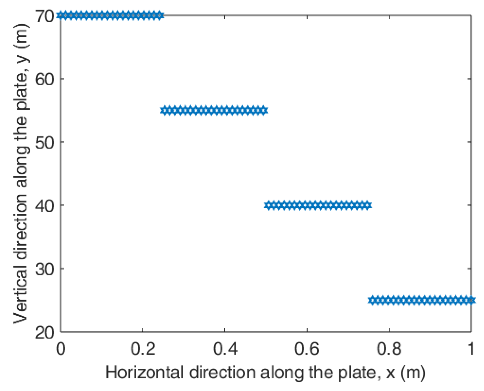
Figure 15.
Temperature distribution with piecewise convection coefficient steady state, Fluent result.
Figure 15.
Temperature distribution with piecewise convection coefficient steady state, Fluent result.
Figure 16 illustrates the temperature results from the Fluent solver. Temperatures increase as the convection coefficient is reduced to the right of the domain.
Figure 17 illustrates the novel solver results for the temperature field. The values are very close to the Fluent results, with a mean relative difference less than 1%. Since the solver yields results very close to the analytical solution, the error could be actually coming from the Fluent solver.
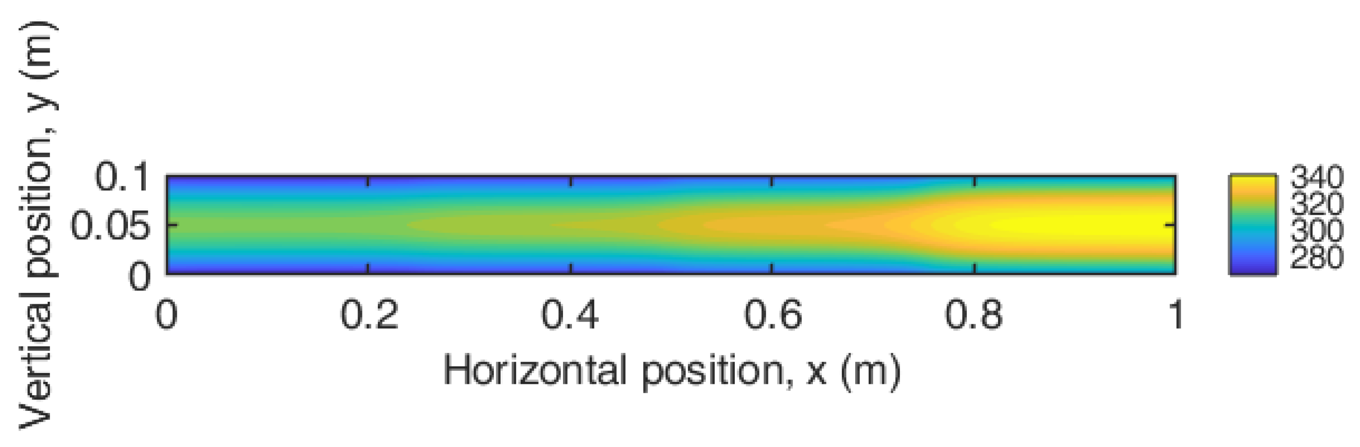
Figure 17.
Temperature distribution with piecewise convection coefficient, steady state, novel solver result.
Figure 17.
Temperature distribution with piecewise convection coefficient, steady state, novel solver result.
An important numerical study is performed to understand effect of curvature of the shell structures of airfoils on the temperature field and whether a flat plate assumption could be used instead of airfoil shell in numerical optimization studies. Toward this end, coordinate transformation depicted in Section 3 is performed. The temperature field obtained by flat plate assumption is compared with that of curved top shell of the NACA 0012 airfoil. The flat plate and shell has been taken with a 1 mm thickness in y direction. The wing shell is assumed to be composed of plies with same orientation. Since the variable investigated is the effect of the curvature on the temperature field, it is not fruitful to have changing ply orientations in this analysis. Chord length of the airfoil is taken as 1 m. To keep the matters simple and focus on the effect of curvature, convection coefficient is taken as constant at h=50 W/m2K with Tinf=253 K as before. Bottom edge is insulated and left and right edges are kept at 273 K. Density, specific heat capacity, and conductivity values are kept the same with orthotropic material properties. Various heat generation rates are investigated. The domain is discretized with 100x103 cells after a mesh independence study. The thin shell structure necessitates a higher power density to provide similar energy levels as before inside the body. 2D, steady, incompressible thermal simulations are performed. Iterations are performed till root mean square error in the temperature field is below 10-8. Domain of interest for the 2D airfoil shell structure is given by Figure 18. Only the upper half of the body is investigated which is sufficient to show the close similarity between flat plate and airfoil shell. Only a minor change in results can be expected with the addition of lower half of the airfoil to the analysis, especially at zero angle of attack.
Obtained temperature field for the shell structure is given by Figure 19 for 1x10⁶ W/m3 heat generation rate. To provide a better visibility of the temperature distribution inside the shell y axis is enlarged. The temperatures are in the safe region.
The same analysis is performed for a rectangular plate of 1 m x 0.001 m, to see the effect of curvature on the temperature distribution. The temperature difference is less than 0.1 K. The reason of low discrepancy between the two geometries comes from the overall low curvature of the airfoil. This validates the approach to utilize flat plates in the next section as substitute for airfoil curved shells. Figure 20 illustrates the results for rectangular plate of similar dimension compared to airfoil shell. The results are very close to each other.
To further analyze the matter, different heat generation rates are also utilized. Heat generation rates of 2.5x10⁶ W/m3, and 3x10⁶ W/m3 are also utilized for the simulations.
Figure 21 and Figure 22 illustrate temperature distribution for the airfoil shell structure and rectangular plate respectively. Results are very close with less than 0.1 K discrepancy and above icing temperatures.
Figure 23 and Figure 24 illustrate temperature distribution for the airfoil shell structure and rectangular plate respectively. Again, very close values with less than 0.1 K discrepancy are obtained for temperatures between airfoil shell and rectangular plate. Temperatures increased with the increase in heat generation.
Note that the energy inputs utilized in this analysis corresponds to the same amount of net energy input for the plates (1x0.1 m) investigated previously. Unit length in the depth direction can be used to obtain the final unit of Watts.
5. Optimization Studies
Gradient-based and evolutionary optimization techniques are widely employed in engineering optimization problems. While gradient-based methods can be effective for smooth and well-conditioned objective functions, their applicability is limited in highly nonlinear problems involving multiple design variables and complex response surfaces. In contrast, evolutionary algorithms do not require gradient information and are therefore particularly advantageous for strongly nonlinear and multimodal optimization problems.
In the present study, a genetic algorithm, which is a class of evolutionary optimization techniques, is implemented [34]. Genetic algorithms have been shown to be highly effective for solving complex nonlinear engineering problems [35,36] The optimization studies are carried out using the Genetic Algorithm Toolbox available in MATLAB R2024a. A schematic overview of the overall genetic-algorithm-based optimization workflow is presented in Figure 25.
For the following optimization studies, the cross-over fraction is selected as 0.8, meaning 80% percent of the current population is transferred to the next generation with inter-changes. For the crossover function, crossoverscattered’ is utilized for each possible selection decision. In the randomly formed binary decision vector, a 1 value corresponds to the selection from the first parent, and a zero value implies selection from the second parent. The algorithm then combines the genes to form the child. For example, if p1 and p2 are the parents;
p1 = [h g f t u o j k]
p2 = [10 20 30 40 50 60 70 80]
If the binary vector is [1 0 0 0 1 0 0 0], the crossover operation yields:
child1 = [h 20 30 40 u 60 70 80]
For the following optimization studies, ‘mutationgaussian’ function is used which adds a random number taken from a Gaussian distribution with average 0 to each entry of the parent vector. The amount of mutation changes proportional to the standard deviation of the fitness function distribution obtained in the optimization run. The ga default selection function, ’selectionstochunif’ is utilized. Parents are chosen based on fitness, but in a way that is less random than simple roulette-wheel selection. Fitter individuals get more chances of selection. At each step, the selection algorithm allocates a parent from the chromosome where each population member is represented proportional to its scaled fitness value.
5.1. Optimization for the Correlation Relation for the Convection Heat Transfer Coefficient
To describe the complex behavior of the convective heat transfer coefficient as observed in Figure 3, a correlation equation is developed using the genetic algorithm. An analytical equation form is first proposed based on flat-plate heat transfer analogy and the expected mathematical behavior of the solution. The coefficients of the proposed correlation are then determined through genetic algorithm optimization to accurately represent the CFD-derived convection heat transfer data.
x’=x/c;
The coefficients r1, r2, r3 are determined using the genetic algorithm based on the convective heat transfer data obtained from the RANS simulations. Once identified, the resulting correlation can be directly implemented in subsequent heat transfer analyses to represent the chordwise variation of the convective heat transfer coefficient.
To this end, the genetic algorithm is executed with a population size of 100, a maximum of 1000 generations, and an elite member count of one. These algorithm-related parameters are selected to ensure sufficient exploration of the design space while maintaining convergence stability.
The optimized correlation obtained from the genetic algorithm is expressed as follows:
The 10 coefficient inside the sin() helps maximize the function close to the 0.1*chord length. The exponential function helps resolve the decay behavior after the leading edge section. In the leading edge section, interaction of fluid particles with the solid wall is higher, while after a certain length along the chord line this interaction and accompanying heat transfer is reduced as the impingement of the flow on the solid wall is significantly lowered. The convective heat transfer coefficients predicted by the proposed correlation are compared with the corresponding RANS simulation results for Reynolds numbers ranging from 9.4 × 10⁵ to 3.12 × 10⁶. This range is selected to represent flow conditions typically encountered by small-medium unmanned aerial vehicles [32]. The comparison demonstrates close agreement between the correlation-based predictions and the CFD results across the entire Reynolds number range considered. The validation results are presented in Figure 26, Figure 27 and Figure 28 for NACA 0012 airfoil.
The validation results are presented in Figure 29, Figure 30 and Figure 31 for NACA 0015 airfoil. Overall, model accuracy is very good. It is much better to model using the developed relation than assuming a constant h value. As expected, h increases as Re increases.
The validation results are presented in Figure 32, Figure 33 and Figure 34 for NACA0018 airfoil. The developed model equation yields results close to the RANS simulation. The results are close to those obtained previously for NACA 0012, and NACA 0015 airfoils at each Reynolds number investigated.
To understand the improvement obtained, results are compared with the flat plate correlation [37]. For turbulent flow with Pr=0.71, Re=9.4E5, k=0.0242 W/mK, L=1 m, h coefficient is given as;
At the 0.1*chord length Re=9.4E5, for NACA 0018 airfoil, mean percent relative error when comparing RANS simulations to flat plate correlation is 33.8%. The mean percent relative error is reduced to 6.4% by the correlation equation developed in this study. This is a significant improvement.
Convergence plot for the optimization study is given by Figure 35. The score equates to the summation of relative errors of h that is calculated over 7200 data points. The optimization starts from a relatively high percent error, but error rapidly diminishes.
5.2. Optimization for the Heater Geometry and Power Input
The composite plate is modeled as a laminate consisting of stacked plies with uniform angular orientation at 00. The thermal problem described in Sections 3.2 and 3.3 are adopted as the basis for the present optimization study, with the computational domain extended to 10 m × 1 m to capture the effects of heater geometry and placement more comprehensively. Buckypaper is selected as the heater material due to its favorable electrothermal properties [38]. Two internal heater bands are incorporated to promote uniform temperature distribution within the composite plate. Orthotropic thermal properties are assigned to the composite material, and a medium-thermal-conductivity surface composite is included on the external surfaces to enhance heat transfer from the interior to the surface.
Geometries in the upcoming optimization study is different compared to an airfoil shell to simplify the meshing process and reduce computational cost. While the geometries under study in the upcoming sections are relatively different compared to the airfoil shell, they can be used to infer the information about the electrothermal design requirements for the airfoil shell. This can be described by the following steady state temperature equation for a 2D plate:
where W and H corresponds to width and height of the plate, respectively.
The equation above indicates that if egen*H ration is maintained, the resultant steady state temperatures will be similar. So, if instead of 1 (m), 1E-3 [m] is used for the value of H, the egen should be multiplied by a factor of 1E3. The equations given above are valid for the steady state temperatures. In the transient simulation at the interim time, the thinner plate with lower H will reach the steady state faster since the time constant increases proportional to H parameter, and increase in the time constant leads to slower change of temperature [33].
Since the heat loss by convection calculation for the plates in the following analyses is directly coming from the non-dimensionalized convection correlation equation of airfoils and not from a plate analysis, the only factor that needs adjustment is the amount of heat generation inside the airfoil, which can be adjusted to satisfy the equality in Eq. (24), hence ensure the similar thermal behavior for the airfoil and plate.
The optimization problem is formulated with four design variables. The volumetric heat generation rate within the heater bands (variable 1) is allowed to vary between 1.0 × 10³ and 2.0 × 10⁴ W/m3. The heater band width (variable 2) is constrained to discrete values ranging from 5 cm to 25 cm in increments of 5 cm.
The x direction in the 2D simulations corresponds to the transverse(across the chord) in-plane direction in 3D composite wing structure which is formed by 0 degree plies. The thermal conductivity range for the optimization study in the x direction (variable 3) is [0.6 0.8] W/m·K. The lower bound and upper bound for the conductivity are obtained by using Eqn. (2), and implementing the parameter settings (kf=1 W/mK, km=0.25-0.5 W/mK, vf=0.7). Lower values for the matrix conductivity can be easily obtained with the use of epoxy as the matrix material. The higher values for matrix conductivity can be obtained by using a highly conductive filler (SiC, alumina etc.) Since the conductivity of these filler particulate materials are in general at least 100 times higher than that of epoxy resin, such matrix conductivity values can be obtained at low filler concentrations [39,40].
The y direction in the 2D simulations corresponds to the through the thickness direction in 3D composite wing structure. For GFRP, as measured experimentally, transverse conductivity, and through the thickness conductivity is very close to each other [41]. This situation is entirely different for CFRP, where through the thickness conductivity is much lower compared to in-plane conductivities due to anisotropy of the fiber material [42]. In this study, ky= 0.9*kx utilized due to quasi isotropic nature of glass fibers. The exact value of the ky will depend on many factors including curing pressure, manufacturing method, and surface treatment [43].
The heating time is restricted to 6 minutes. Hence, this is basically a de-icing operation.
Finally, the thermal conductivity of the external surface protection material (variable 4) is optimized within the range of 1 to 10 W/m·K. There are boron nitride &epoxy matrix composites that provide thermal conductivities in this range while being electrical insulator [44].
Because the heater width directly affects the computational mesh, a variable transformation strategy is employed to avoid excessive remeshing and impractical geometric configurations. The heater width optimization interval is first mapped onto an integer variable domain, and an integer constraint is enforced during optimization. Each integer value corresponds to a predefined heater width and an associated mesh parameter, ensuring consistent grid topology throughout the optimization process. The transformation is defined as
var2<=>widthheater
var2 ∈ [15 16 17 18 19]
widthheater ∈ [5 10 15 20 25) [cm]
Code structure utilized for the transformation is given below.
if var2==15
widthheater =25 cm
segen=7 (bounding upper node of the heating region)
elseif var2==16
widthheater =20 cm
segen=6
elseif var2==17
widthheater =15 cm
segen=5
elseif var2==18
widthheater =10 cm
segen=4
elseif var2==19
widthheater =5 cm
segen=3
end
The transformation explained above makes the optimization process computationally more efficient and stable as remeshing requirements are optimized, and impractical real numbers for heater width is avoided where meshing with quad and even triangular elements could pose problems.
During the optimization, a population size of 32 is maintained for 200 generations. In each generation, 1 elite member is directly transferred to the next generation without any modification. The initial values for the optimization variables [r1, r2, r3, r4, r5] are selected as [2x10³ W/m3, 15 cm, 0.8 W/m.K, 0.7 W/m.K, 10 W/m.K] Although these initial values are arbitrarily chosen, they satisfy the genetic algorithm’s requirement for an initial feasible solution.
During the optimization, the upper and lower surfaces of the plate are subjected to convective heat transfer relation obtained in the previous optimization study. The left and right boundaries are prescribed as isothermal surfaces at 273 K. Two heater bands are embedded near the upper and lower surfaces of the composite plate. Reynolds number of 1.0 × 10⁶ is assumed in the simulation.
The electrothermal heater is modeled as buckypaper. The thermal conductivity of the heater material is assumed to be isotropic, with values of 2.5 W/m·K in both the streamwise (x) and transverse (y) directions.
As a central contribution of this study, a novel objective function is formulated to guide the optimization of the electrothermal heating system.
To prevent excessive heating under both constant and spatially varying convective heat transfer conditions, an additional safety mechanism is incorporated into the genetic algorithm framework. Specifically, if the maximum temperature within the composite domain exceeds a prescribed threshold, the corresponding design is heavily penalized by assigning a large fitness value. This approach ensures that thermally unsafe configurations are systematically excluded from the optimization process. The penalty strategy is implemented as
if abs(max(T(:)))>=323
fitness value=1E6
else
fitness value=objective function
The objective function is formulated to achieve multiple competing goals. It is aimed to keep the surface temperature at the top and bottom surfaces at 277 K to prevent icing conditions. Hence, the first two terms in the objective function are shaped. A design deviation temperature difference (taken as 1 K) is introduced into the denominator. To provide enough penalty for designs away from this point, exponent 3 and absolute operations are introduced. The third term has the goal of minimizing the power consumption and it is normalized with minimum power consumption for the problem (1 kW/m3). The last term is formulated to avoid the occurrence of excessive temperatures on the composite plate. The formulation of the objective function is non-dimensionalized.
In the present study, the heater bands (buckypaper) and the protective surface material were modeled as perfect thermal conductors with ideal bonding to the composite substrate. This assumption was intentionally adopted to reduce model complexity and computational cost, and to focus the optimization framework on the influence of heater placement, geometry, and power distribution on the global thermal response. Under this assumption, the predicted temperature field represents an upper-bound heat-spreading capability of the system.
In practical implementations, the interfaces between the buckypaper heater, the composite laminate, and the surface protection material may introduce finite thermal contact resistance due to surface roughness, incomplete wetting, and interfacial defects. Such resistances can locally impede heat transfer and potentially lead to higher peak temperatures and localized hot spots. Consequently, neglecting interfacial thermal resistance may result in an underestimation of maximum internal temperatures and an optimistic prediction of thermal uniformity.
However, the optimization trends identified in this work—such as the relative effectiveness of heater configurations and power distributions—are expected to remain valid, as thermal contact resistance would primarily introduce a uniform temperature offset rather than altering the comparative performance between optimized designs.
Furthermore, a margin of 4 K is introduced in the objective function that will compensate for the thermal contact related temperature deviations. The materials utilized for heater material (buckypaper) adhere to the resin and glass fiber very well under correct manufacturing conditions, leading to minimal thermal contact resistance.
Convergence plot is given by Figure 36. The solution rapidly converges to the optimum solution.
Upon completion of the optimization process, the optimal design parameters are inserted into the thermal solver to evaluate the resulting temperature field. The optimized temperature distribution is presented in Figure 37. The results demonstrate that the surface temperatures remain above the icing threshold while excessive internal temperatures are effectively avoided, validating the effectiveness of the proposed objective function and optimization framework.
The design variables are optimized using the genetic algorithm described in the previous section. The optimal values obtained for the design variables are summarized in Table 1.
In order to evaluate the reliability and performance of the optimized electrothermal heating configuration and quantify the relative influence of individual design variables, a sensitivity analysis was conducted around the optimal solution obtained from the genetic algorithm based optimization. The objective of this analysis is to identify the dominant parameters governing the thermal response and assess the sensitivity of the optimization outcome to variations in design variables.
The sensitivity analysis was performed using a one-at-a-time perturbation approach. Each design variable was independently perturbed while all other variables were held fixed at their optimized values. For continuous variables, perturbations of ±10% about the optimal value were applied.
The baseline optimized design corresponds to a volumetric heat generation rate of 1271 W/m3, a heater width of 25 cm, an in-plane composite thermal conductivity of 0.6 W/m·K corresponding to transverse direction for a mapped 3D wing body, a conductivity of 0.54 W/m.K corresponding to the out-of plane direction for a mapped 3D wing body, and a surface protection material thermal conductivity of 10 W/m·K. For each perturbed case, the thermal solver was executed using identical boundary conditions and convective heat transfer relations as those employed during the optimization process.
Table 2 presents the findings of the sensitivity analysis. Performed sensitivity analysis confirms that the optimized heating configuration is reliable and provide superior performance.
Only small changes are observed by a change of the optimization variables. Perturbation in all the cases lead to lower surface temperature, indicating the superior performance of the optimum design obtained from genetic algorithm. Interestingly, an increase of GFRP thermal conductivity directs the heat inwards away from the surface for the current design, hence it actually drops the surface temperatures. If heaters are located away from the surface, this effect will be reversed, and higher conductivity of GFRP will be crucial.
Calculations during the optimization are parallelized to 30 workers using a 16-core & 32 thread Intel Ryzen 5950X processor.
5.3. Optimization for the Heater Geometry, Power Input and Ply Angles
Same configuration given in Optimization Study 2 is used in this optimization study, except the 0 degree uniform plies are replaced with a ply orientation angle selected as an optimization variable. Effective thermal conductivities are calculated based on the ply angle.
The optimization problem is formulated with four design variables. The volumetric heat generation rate within the heater bands (variable 1) is allowed to vary between 1.0 × 10³ and 2.0 × 10⁴ W/m3, specified as an integer variable. The heater band width (variable 2) is the second integer variable, with values ranging from 5 cm to 25 cm in increments of 5 cm.
The heating time is restricted to 6 minutes. Hence, this is basically a de-icing operation.
The thermal conductivity in the x direction (variable 3) is formulated based on the ply angle [0 45] degrees and transformation relation as given by Eqns. (1)-(4). It translates to the conductivity interval of [0.55 0.65] W/m.K in the x direction. Conductivity in they direction is defined using the same relation in the previous study. It is the third integer variable. Choice of integer variables help ease computational burden, while yielding design variables that can be easily transferred to manufacturing process. Finally, the thermal conductivity of the external surface coating material (variable 4) is optimized within the range of 1 to 10 W/m·K, as in the case of previous study.
The design variables are optimized using the genetic algorithm described in the previous section. The optimal values obtained for the design variables are summarized in Table 3. The 0 degree plies result in lower transverse conductivity, which translate to a higher temperature for a given internal heat generation rate.
Due to excessive computational burden, a ply by ply optimization has not been performed. However, results already indicate favorable ply angle. The optimized temperature distribution is presented in Figure 38. The results again demonstrate the effectiveness of the proposed objective function and optimization framework.
Convergence plot is given by Figure 39. Again, the solution rapidly converge to the optimum solution.
5.4. Optimization for the Heater Geometry, Power Input and Varying Ply Angles for an Anti-Icing System
The optimization study is performed with ply angles, heat generation rate inside the body, and surface conductivity as optimization variables. Surface conductivity can be adjusted by using different materials at the design stage. The domain size (10 m x 1 m) as in the previous case is utilized.
In this case, heating duration is not restricted, and the system is allowed to reach steady state. Such a configuration corresponds to the anti-icing system operation, while the previous optimization studies given in Section 5.2 and Section 5.3 are time restricted and hence corresponds to de-icing operation.
The stacking sequence is [surface coating material (1)-heater-ply 1 (material 2)- ply 2 (material 3)-ply 1 (material 4)—heater (material 5)- surface material (material 6) ] from top to bottom. The heater thickness is taken as 45% of the thickness of the composite plate. The surface coating is 5% of the thickness of the composite plate. The remaining 50% thickness of the composite is thought to consist of composite laminates.
There are four optimization variables in the genetic algorithm function. The first one is the heat generation rate, the second and the third are ply angles, and the final one is the thermal conductivity of the surface coating material. Heat generation rate is allowed to vary between 0 to 20 kW/m3. Ply angles are allowed to vary between 0- 90 degrees. Thermal conductivity of the surface coating material is allowed to vary between 0 to 10 W/m.K. Integer constraints are applied for the heat generation rate and ply angle variables to limit the computational space with the physically applicable input values. The normalized objective function given by Eq. (26) is utilized again. For the genetic algorithm settings, a population size of 32 is utilized for 200 generations. A single elite best performing member is preserved for directly transferring to the next generation. Cross over fraction is kept at 0.8. The crossover, mutation, selection functions are preserved with respect to previous runs as described at the start of Section 5.
Upper and lower edges are subjected to convective heat transfer. Convective heat transfer coefficient is locally changing as per the newly developed correlation equation given by Eq. (21) for Reynolds number of 1 million. The left and right edges are maintained at constant temperature of 273 K.
The variables given in Table 4 are obtained as a result of the optimization run.
Temperature distribution is given by Figure 40 which shows that away from the high convection region, temperatures reach higher levels due to heating.
Convergence history is given by Figure 41. The solution rapidly converges to the final solution.
6. Conclusion
Preventing icing on external wing surfaces is essential for the aerodynamic performance and operational safety of aerial vehicles, particularly unmanned aerial vehicles (UAVs), where composite materials are widely used. For composite wing structures, electrothermal heating remains the most practical and effective approach for de-icing and anti-icing applications.
In this paper, a comprehensive study involving the thermal analysis and optimization of electrothermal heating systems in composite plate structures which represent composite airfoil structures was performed. Thermal performance was initially examined to establish heat generation requirements under varying convective heat loss conditions.
An in-house thermal solver was subsequently validated against a commercial finite volume solver, with less than 1% discrepancy between the results obtained.
To improve the fidelity of heat transfer modeling, a new correlation for the convective heat transfer coefficient was derived using a database of 108 RANS-based flow simulations coupled with a genetic algorithm. The correlation equation is able to reduce the mean percent relative error for the local convection heat transfer coefficient from 33.8% to mere 6.4%. This represents a substantial improvement in predictive accuracy. The use of locally varying convection coefficient in the thermal analyses eliminates the conventional assumption of constant convection coefficient and captures local thermal variations. To the authors’ knowledge, this is the first study to employ an evolutionary algorithm to derive convection heat transfer correlations for electrothermal anti-icing applications on airfoils.
The present study proposes a novel unified optimization approach and introduction of a novel objective function for electrothermal heating systems in composite wing structures. It targets both minimization of power consumption which is very important from the efficiency perspective, and keeping the temperatures at an acceptable range. The current objective function provides physically balanced designs compared to a simple error-based objective function. Excessive temperatures may lead to material degradation or structural failure, and the important target of ensuring a safe and uniform temperature distribution within the composite domain was achieved.
The utilization of buckypaper inside the composite along with a surface coating material is thoroughly simulated which is not extensively covered in the literature. This configuration addresses both the above freezing point surface temperature requirement and fragility of the buckypaper as a surface material. Furthermore, introduction of the heater thickness as an optimization variable helps study thermal uniformity effects.
The study also includes proof-of-concept introduction of lamina ply angles as optimization variables for the electrothermal system optimization on the composite structures. This matter is generally not covered in the existing optimization studies for electrothermal heating systems due to associated high computational costs.
The study utilizes 2D plates as substitute for the composite curved shells. With thin shells, and high curvatures, this is usually a valid assumption as it is demonstrated numerically at the end of Section 4. However, if effective thickness of the wing structure is increased through the introduction of structural elements (honeycomb, stiffeners etc.) the accuracy of the current plate simplification will deteriorate.
Although ply orientation is briefly studied as part of the optimization studies, it is not fully covered in this study. The reason for this comes from the excessive computational burden associated with the ply-by-ply thermal modelling. As each ply orientation introduces a new optimization variable, the optimization becomes a burdensome task if more than a few ply orientations are incorporated as optimization variables.
As part of the study, key design variables, including heater power, heater geometry, and material thermal properties, were systematically optimized. The resulting designs achieved near-target temperature distributions with minimum power input.
The results demonstrated that incorporating unified objective formulations significantly improves the design quality and energy efficiency of electrothermal heating system. The proposed methodology provides a reliable design approach that can be readily extended to three-dimensional composite wing configurations operating under high-altitude, cold-flow conditions.
Author Contributions
DP: Conception, Data Collection, Data Analysis, Writing, Literature review; BP: Conception, Data Collection, Data Analysis, Writing, Technical Support; HA: Conception, Data Analysis, Technical Support, Critical Review of Content.
Funding
This work was supported by the Selcuk University Scientific Research Projects Coordinatorship with project number 24211011.
Data Availability Statement
The data that supports the findings of this study are available from the corresponding author upon reasonable request.
Acknowledgments
This article is a significantly revised and expanded version of a conference paper entitled Thermal Analysis and Design of Composite Structures under Realistic Flow Conditions which was presented at 7th International Conference on Engineering Technologies (ICENTE’23) conference held in Konya/Turkiye between 23-25 November 2023.
Conflicts of Interest
The authors declare that they have no known competing financial interests or personal relationships that could have appeared to influence the work reported in this paper.
References
- Gent, R.W.; Dart, N.P.; Cansdale, J.T. Aircraft Icing. Philosophical Transactions: Mathematical, Physical and Engineering Sciences 2000, 358, 2873–2911. [Google Scholar] [CrossRef]
- Myers, T.G. Extension to the Messinger Model for Aircraft Icing. AIAA Journal 2001, 39, 211–218. [Google Scholar] [CrossRef]
- Schutzeichel, M.O.H. Multiphysical and multi scale modelling of composite materials for aircraft De-Icing. 2023. [Google Scholar]
- Kang, J.; Kim, H.; Kim, K.S.; Lee, S.K.; Bae, S.; Ahn, J.H.; Kim, Y.J.; Choi, J.B.; Hong, B.H. High-performance graphene-based transparent flexible heaters. Nano Lett 2011, 11, 5154–5158. [Google Scholar] [CrossRef] [PubMed]
- Volman, V.; Zhu, Y.; Raji, A.R.; Genorio, B.; Lu, W.; Xiang, C.; Kittrell, C.; Tour, J.M. Radio-frequency-transparent, electrically conductive graphene nanoribbon thin films as deicing heating layers. ACS Appl Mater Interfaces 2014, 6, 298–304. [Google Scholar] [CrossRef]
- Mohammed, A.G.; Ozgur, G.; Sevkat, E. Electrical resistance heating for deicing and snow melting applications: Experimental study. Cold Regions Science and Technology 2019, 160, 128–138. [Google Scholar] [CrossRef]
- Kim, T.; Chung, D. Carbon fiber mats as resistive heating elements. Carbon 2003, 41, 2436–2440. [Google Scholar] [CrossRef]
- Yoon, Y.-H.; Song, J.-W.; Kim, D.; Kim, J.; Park, J.-K.; Oh, S.-K.; Han, C.-S. Transparent Film Heater Using Single-Walled Carbon Nanotubes. Advanced Materials 2007, 19, 4284–4287. [Google Scholar] [CrossRef]
- Feng, C.; Liu, K.; Wu, J.-S.; Liu, L.; Cheng, J.G.; Zhang, Y.; Sun, Y.; Li, Q.; Fan, S.; Jiang, K. Flexible, Stretchable, Transparent Conducting Films Made from Superaligned Carbon Nanotubes. Advanced Functional Materials 2010, 20, 885–891. [Google Scholar] [CrossRef]
- Chu, H.; Zhang, Z.; Liu, Y.; Jinsong, L. Self-heating fiber reinforced polymer composite using meso/macropore carbon nanotube paper and its application in deicing. Carbon 2014, 66, 154–163. [Google Scholar] [CrossRef]
- Yao, X.; Hawkins, S.; Falzon, B.G. An advanced anti-icing/de-icing system utilizing highly aligned carbon nanotube webs. Carbon 2018, 136, 130–138. [Google Scholar] [CrossRef]
- Park, H.K.; Kim, S.M.; Lee, J.S.; Park, J.-H.; Hong, Y.-K.; Hong, C.H.; Kim, K.K. Flexible plane heater: Graphite and carbon nanotube hybrid nanocomposite. Synthetic Metals 2015, 203, 127–134. [Google Scholar] [CrossRef]
- Aliberti, F.; Sorrentino, A.; Palmieri, B.; Vertuccio, L.; De Tommaso, G.; Pantani, R.; Guadagno, L.; Martone, A. Lightweight 3D-printed heaters: design and applicative versatility. Composites Part C: Open Access 2024, 15, 100527. [Google Scholar] [CrossRef]
- Ibrahim, Y.; Kempers, R.; Amirfazli, A. 3D printed electro-thermal anti- or de-icing system for composite panels. Cold Regions Science and Technology 2019, 166, 102844. [Google Scholar] [CrossRef]
- Roy, R.; Raj L, P.; Jo, J.-H.; Cho, M.-Y.; Kweon, J.-H.; Myong, R.S. Multiphysics anti-icing simulation of a CFRP composite wing structure embedded with thin etched-foil electrothermal heating films in glaze ice conditions. Composite Structures 2021, 276, 114441. [Google Scholar] [CrossRef]
- Mohseni, M.; Amirfazli, A. A novel electro-thermal anti-icing system for fiber-reinforced polymer composite airfoils. Cold Regions Science and Technology 2013, 87, 47–58. [Google Scholar] [CrossRef]
- Laroche, A. Comparative Evaluation of Embedded Heating Elements as Electrothermal Ice Protection Systems for Composite Structures. Masters, Concordia University, 2017.
- Kim, M.; Sung, D.H.; Kong, K.; Kim, N.; Kim, B.-J.; Park, H.; Park, Y.-B.; Jung, M.; Lee, S.; Kim, S. Characterization of resistive heating and thermoelectric behavior of discontinuous carbon fiber-epoxy composites. Composites Part B: Engineering 2016, 90, 37–44. [Google Scholar] [CrossRef]
- Falzon, B.G.; Robinson, P.; Frenz, S.; Gilbert, B. Development and evaluation of a novel integrated anti-icing/de-icing technology for carbon fibre composite aerostructures using an electro-conductive textile. Composites Part A: Applied Science and Manufacturing 2015, 68, 323–335. [Google Scholar] [CrossRef]
- Pourbagian, M. Multidisciplinary Optimization of In-Flight Electro-Thermal Ice Protection Systems. 2015.
- Pourbagian, M.; Habashi, W. Aero-thermal optimization of in-flight electro-thermal ice protection systems in transient de-icing mode. International Journal of Heat and Fluid Flow 2015, 54. [Google Scholar] [CrossRef]
- Wang, T.; Zhang, W.; Chen, J.; Li, S.; Yu, L.; Zhu, D.; Mao, X. Power optimization of the aircraft electrothermal de-icing heaters. Applied Thermal Engineering 2025, 280, 128236. [Google Scholar] [CrossRef]
- Trakakis, G.; Tomara, G.; Datsyuk, V.; Sygellou, L.; Bakolas, A.; Tasis, D.; Parthenios, J.; Krontiras, C.; Georga, S.; Galiotis, C.; et al. Mechanical, Electrical, and Thermal Properties of Carbon Nanotube Buckypapers/Epoxy Nanocomposites Produced by Oxidized and Epoxidized Nanotubes. Materials (Basel) 2020, 13. [Google Scholar] [CrossRef] [PubMed]
- Roy, R.; Raj, L.P.; Jo, J.-H.; Cho, M.-Y.; Kweon, J.-H.; Myong, R.S. Multiphysics anti-icing simulation of a CFRP composite wing structure embedded with thin etched-foil electrothermal heating films in glaze ice conditions. Composite Structures 2021, 276. [Google Scholar] [CrossRef]
- Pourbagian, M.; Habashi, W.G. Aero-thermal optimization of in-flight electro-thermal ice protection systems in transient de-icing mode. International Journal of Heat and Fluid Flow 2015, 54, 167–182. [Google Scholar] [CrossRef]
- Saripally, A. A Micromechanical Approach to Evaluate the Effective Thermal Properties of Unidirectional Composites. 2015. [Google Scholar]
- Affdl; Patterson, W. The Halpin-Tsai Equations: A Review. Polymer Engineering and Science 1976, 16, 344–352. [Google Scholar] [CrossRef]
- Fletcher, C.A. Computational techniques for fluid dynamics 2; Springer-Verlag: 1988.
- Adeyi, T.A.; Alabi, O.O.; Towoju, O.A. Influence of Airfoil Geometry on VTOL UAV Aerodynamics at Low Reynolds Numbers. Archives of Advanced Engineering Science 2024. [Google Scholar] [CrossRef]
- Lee, J.-s.; Jo, H.; Choe, H.-s.; Lee, D.-s.; Jeong, H.; Lee, H.-r.; Kweon, J.-h.; Lee, H.; Shin Myong, R.; Nam, Y. Electro-thermal heating element with a nickel-plated carbon fabric for the leading edge of a wing-shaped composite application. Composite Structures 2022, 289, 115510. [Google Scholar] [CrossRef]
- Pehlivan, D.A., Hasan. Thermal Analysis and Design of Composite Structures under Realistic Flow Conditions. In Proceedings of the 7th International Conference on Engineering Technologies (ICENTE’23) Konya/Turkiye, 23–25 November 2023, 2023; pp. 196–204.
- Cengel. Heat Transfer: A Practical Approach; 2016.
- Incropera, F.P.; DeWitt, D.P. Fundamentals of Heat and Mass Transfer, 4th Edition ed.; John Wiley & Sons, Inc.: New York City, New York, 1996.
- Sampson, J.R. Adaptation in Natural and Artificial Systems (John H. Holland). SIAM Review 1976, 18, 529–530. [Google Scholar] [CrossRef]
- Goldberg, D.E. Genetic Algorithms in Search, Optimization, and Machine Learning; Addison-Wesley: New York, 1989.
- Jong, K.A.D. An Analysis Of The Behavior Of A Class Of Genetic Adaptive Systems. 1975.
- Bahrami, M. Forced Convection Heat Transfer, ENSC 388. 2011.
- Cao, L.; Liu, Y.; Wang, J.; Pan, Y.; Zhang, Y.; Wang, N.; Chen, J. Multi-Functional Properties of MWCNT/PVA Buckypapers Fabricated by Vacuum Filtration Combined with Hot Press: Thermal, Electrical and Electromagnetic Shielding. Nanomaterials 2020, 10, 2503. [Google Scholar] [CrossRef]
- Kaundal, R.; Patnaik, A.; Satapathy, A. Comparison of the Mechanical and Thermo-Mechanical Properties of Unfilled and SiC Filled Short Glass Polyester Composites. Silicon 2012, 4, 175–188. [Google Scholar] [CrossRef]
- Vaggar, G.; Kamate, S.C.; Badyankal, P. A study on thermal conductivity enhancement of silicon carbide filler glass fiber epoxy resin hybrid composites. Materials Today: Proceedings 2020, 35. [Google Scholar] [CrossRef]
- Mutnuri, B. Thermal conductivity characterization of composite materials. 2006.
- Han, S.; Chung, D. Increasing the through-thickness thermal conductivity of carbon fiber polymer–matrix composite by curing pressure increase and filler incorporation. Composites Science and Technology - COMPOSITES SCI TECHNOL 2011, 71, 1944–1952. [Google Scholar] [CrossRef]
- Takizawa, Y.; Chung, D. Through-thickness thermal conduction in glass fiber polymer–matrix composites and its enhancement by composite modification. Journal of Materials Science 2016, 51. [Google Scholar] [CrossRef]
- Moradi, S.; Román, F.; Calventus, Y.; Hutchinson, J.M. Remarkable Thermal Conductivity of Epoxy Composites Filled with Boron Nitride and Cured under Pressure. Polymers 2021, 13, 955. [Google Scholar] [CrossRef]
Figure 1.
Flowchart of the genetic algorithm (GA) based design study.
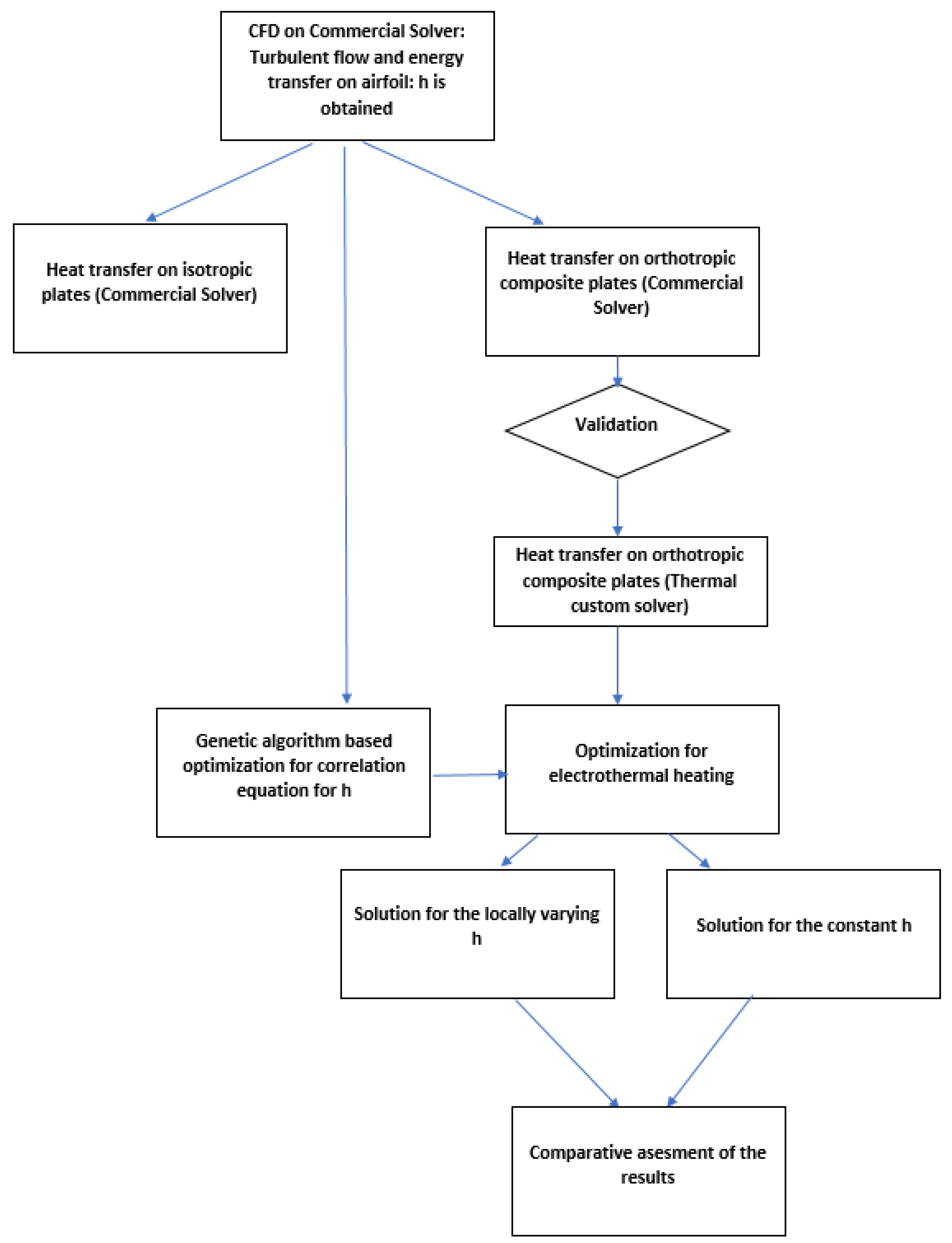
Figure 2.
Grid used in the numerical analysis of flow over airfoils.
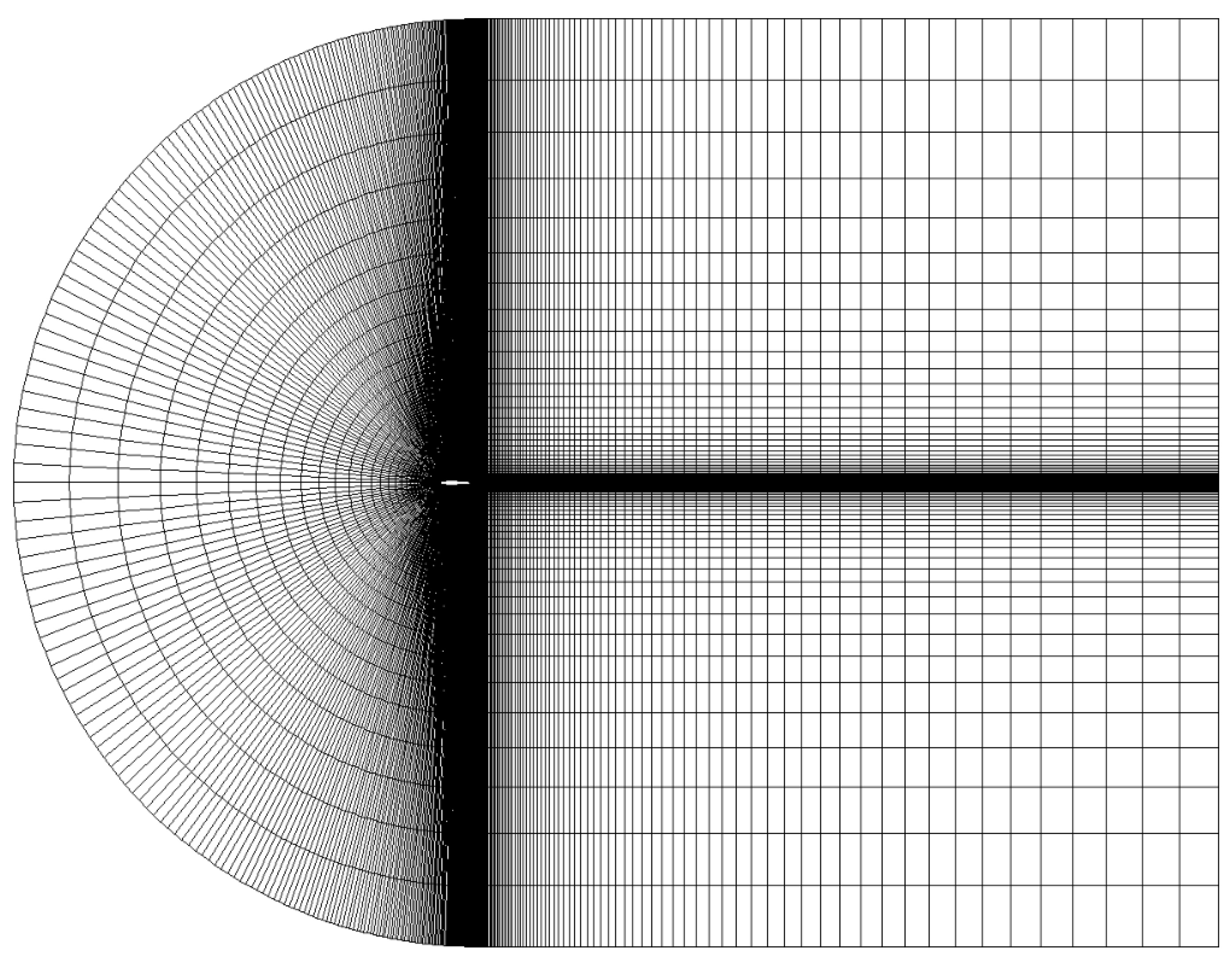
Figure 3.
Chordwise variation of the convective heat transfer coefficient (h) for different Reynolds numbers along the NACA 0012 airfoil surface.
Figure 3.
Chordwise variation of the convective heat transfer coefficient (h) for different Reynolds numbers along the NACA 0012 airfoil surface.
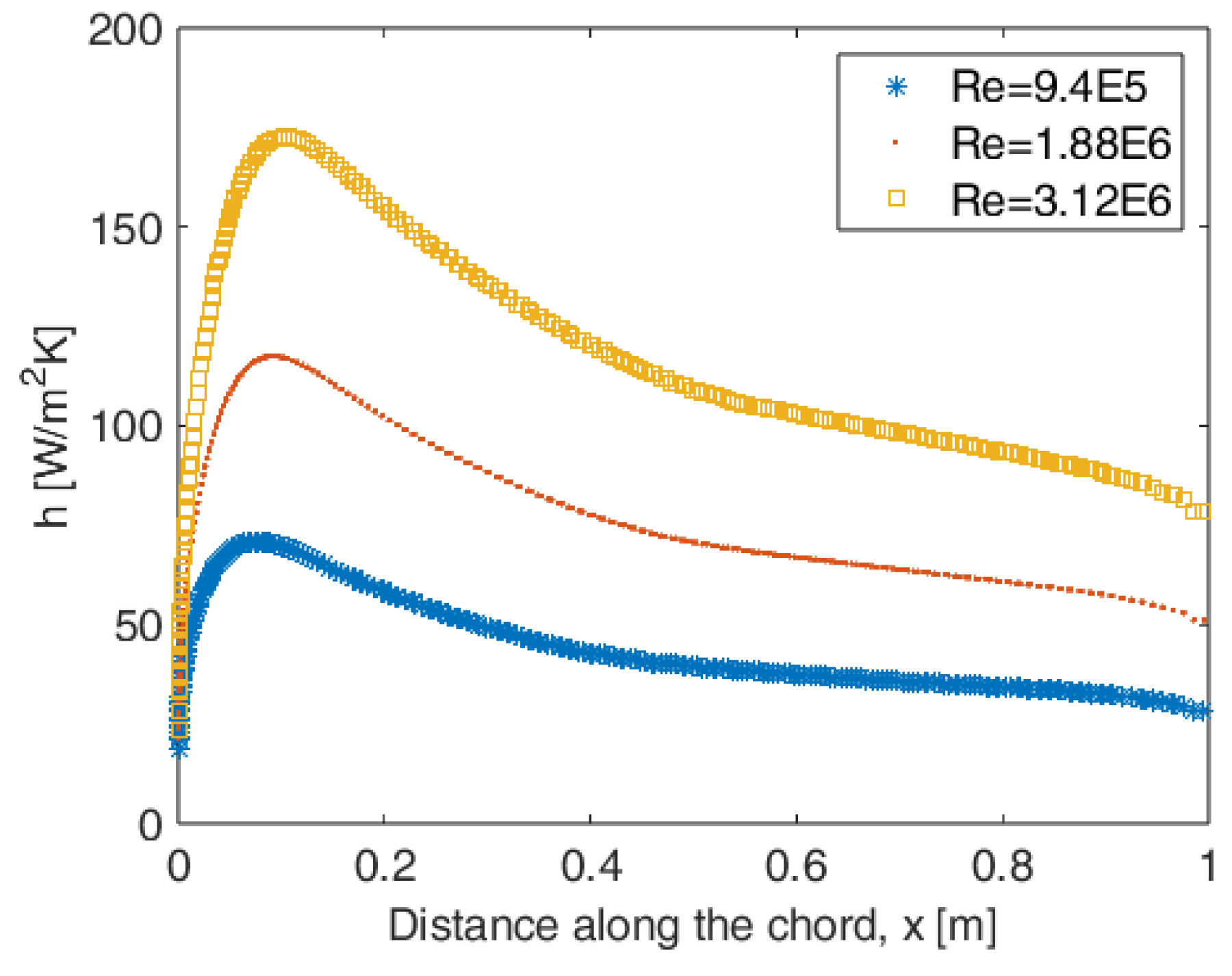
Figure 8.
Temperature distribution predicted by the in-house thermal solver.
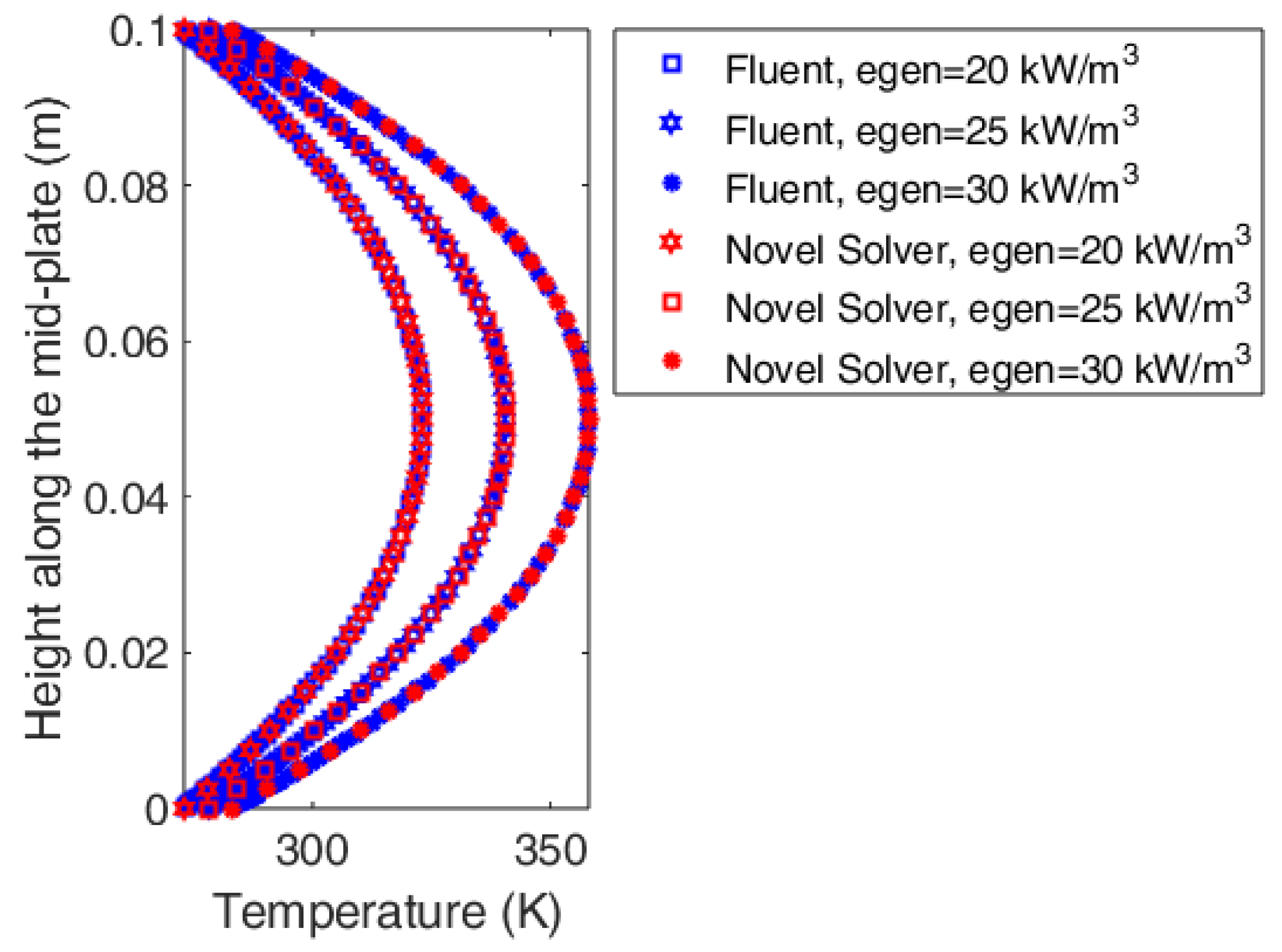
Figure 9.
Mesh independence study for the novel solver at egen=20 kW/m3.
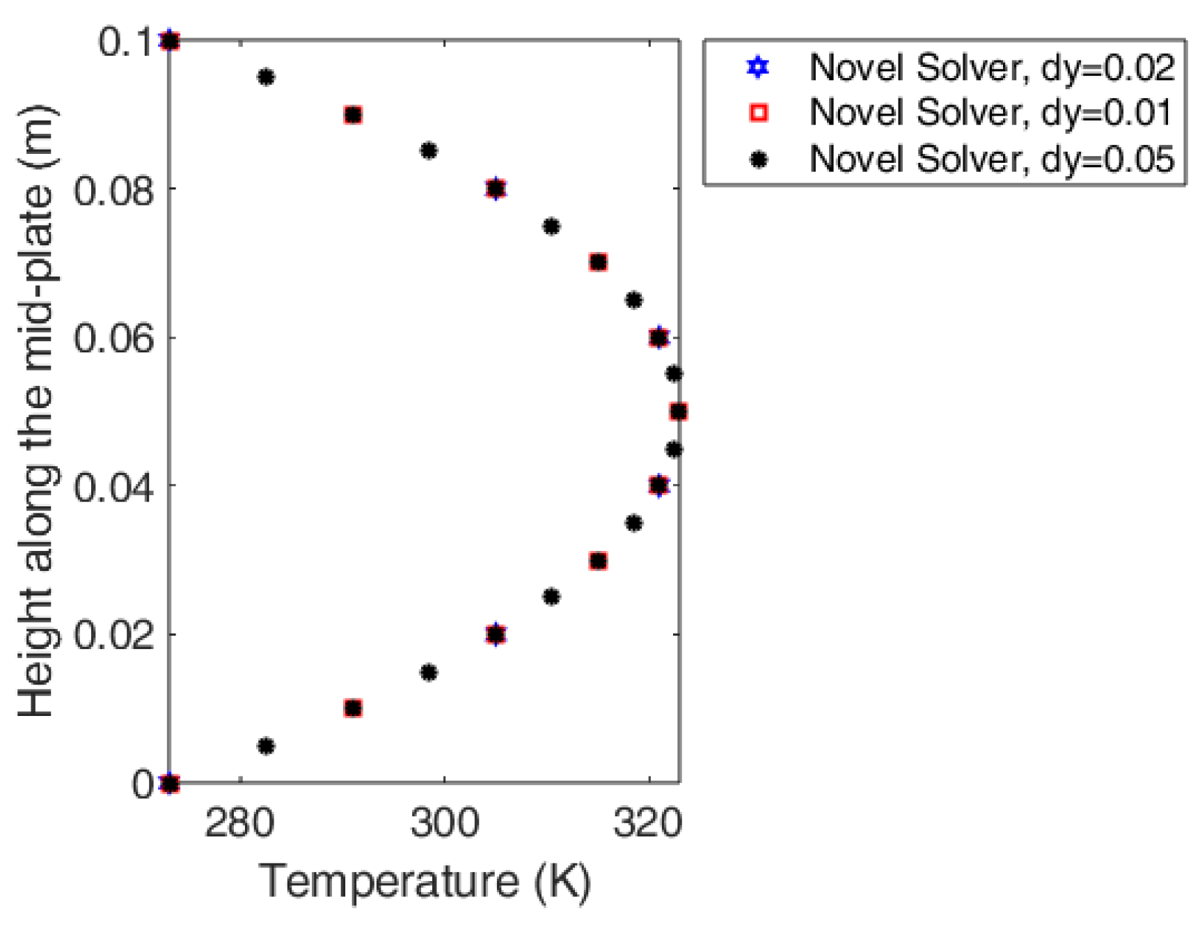
Figure 10.
Temperature distribution predicted by the in-house thermal solver.
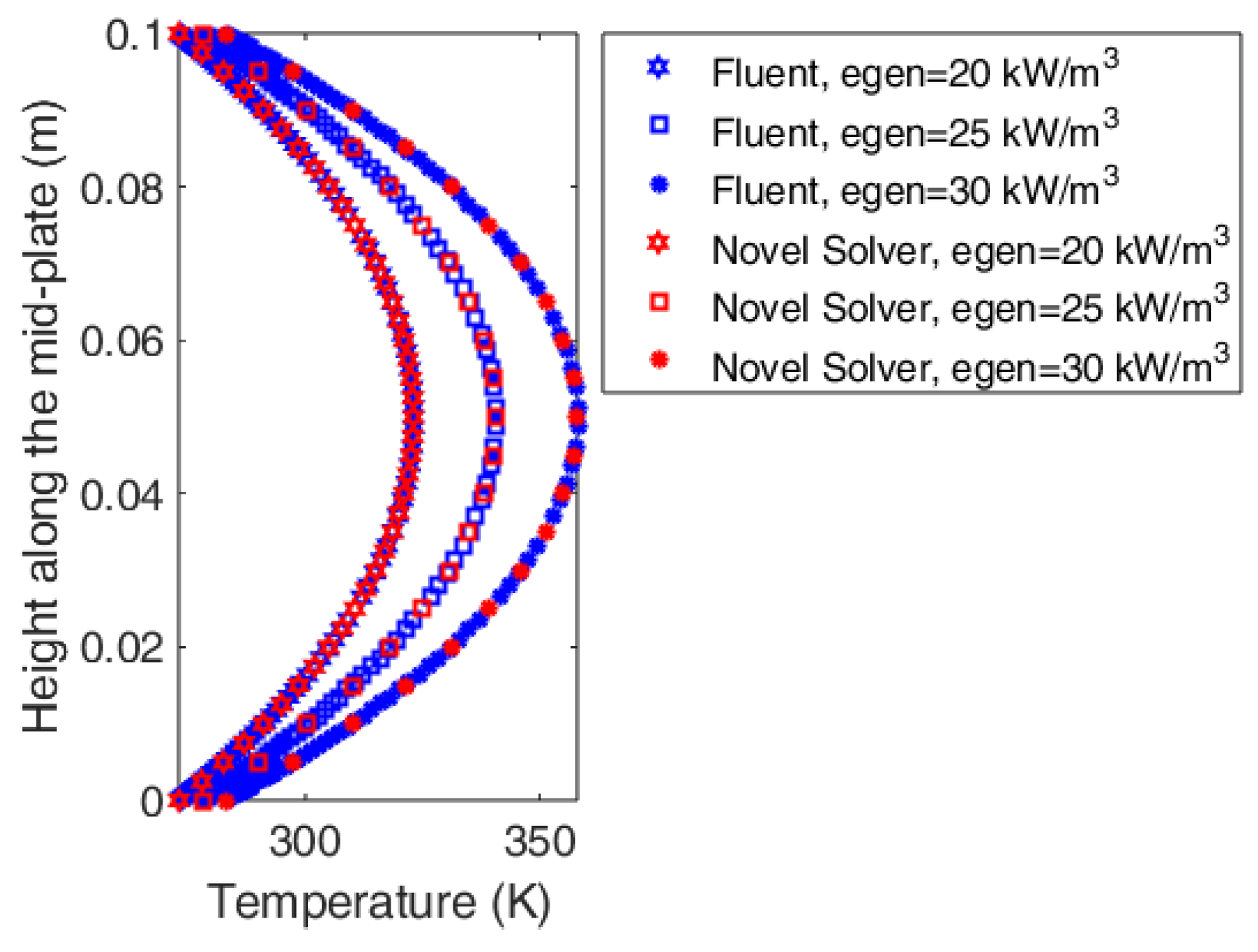
Figure 11.
Temperature distribution for the mesh Fourier number of 0.01.
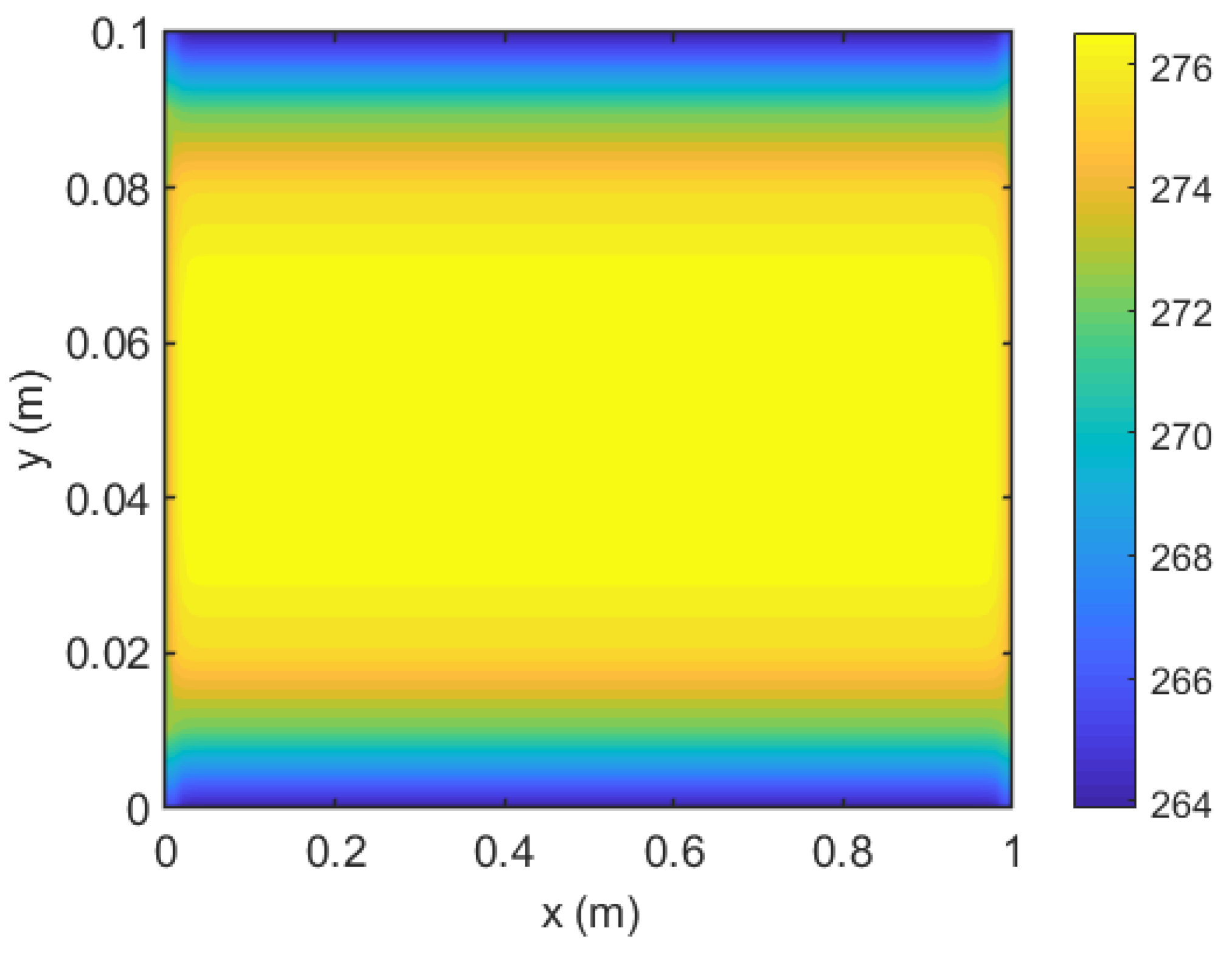
Figure 12.
Temperature distribution for the mesh Fourier number of 0.1.
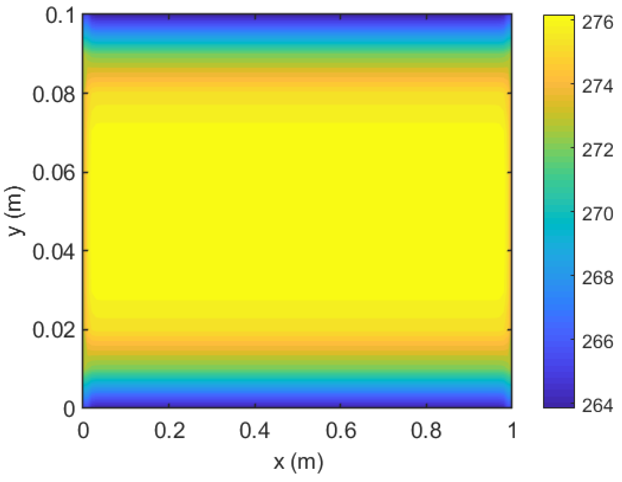
Figure 13.
Temperature distribution steady state, analytical result.
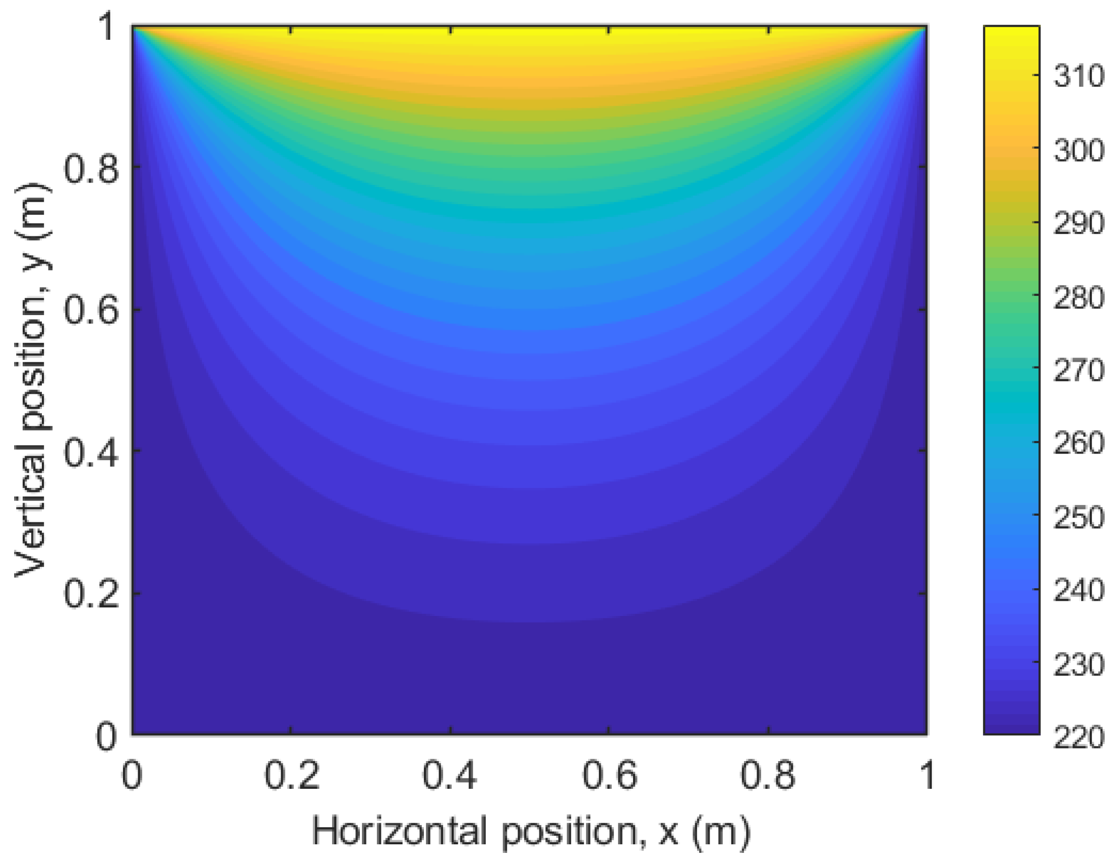
Figure 14.
Temperature distribution steady state, numerical result.
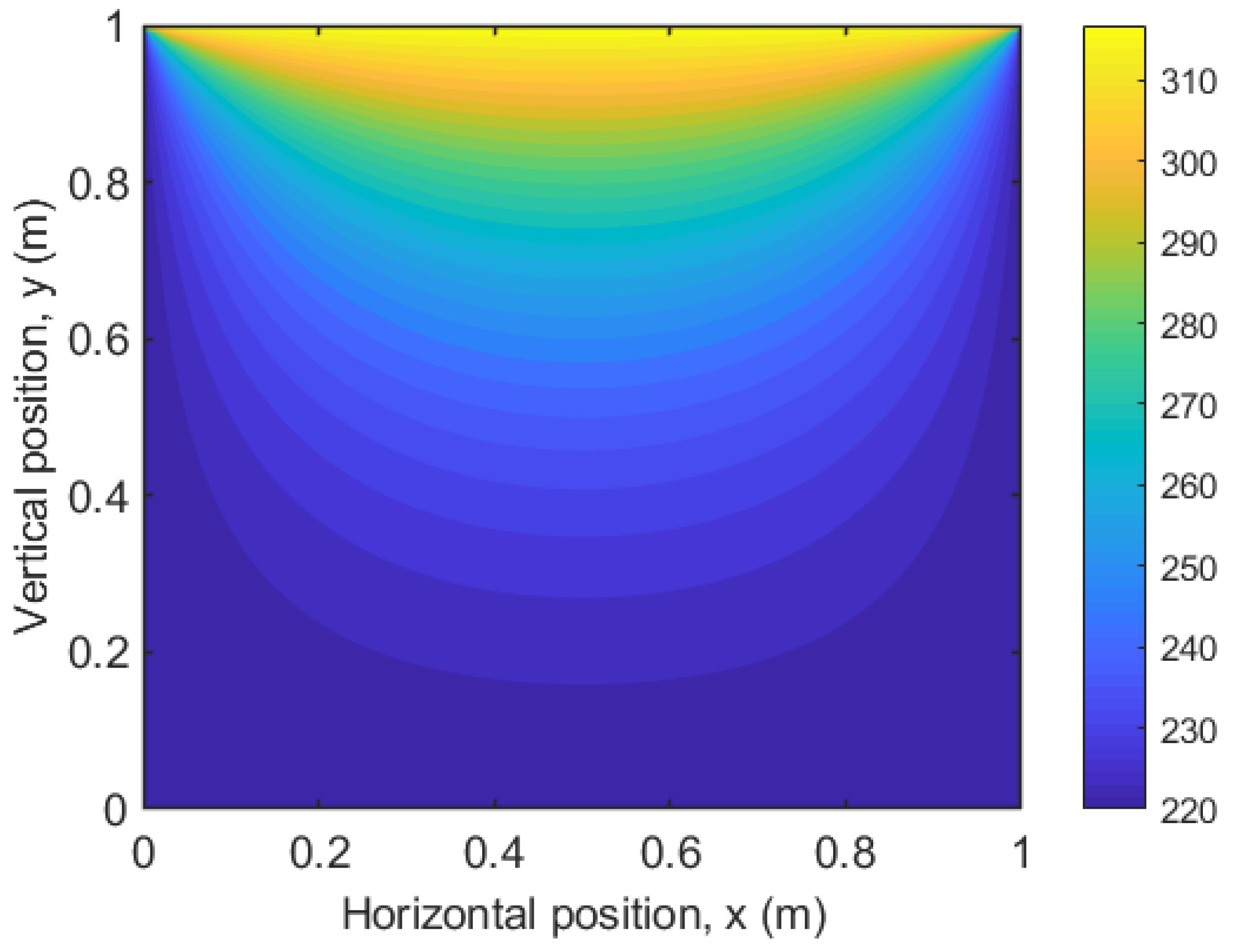
Figure 16.
Temperature distribution with piecewise convection coefficient steady state, Fluent result.
Figure 16.
Temperature distribution with piecewise convection coefficient steady state, Fluent result.
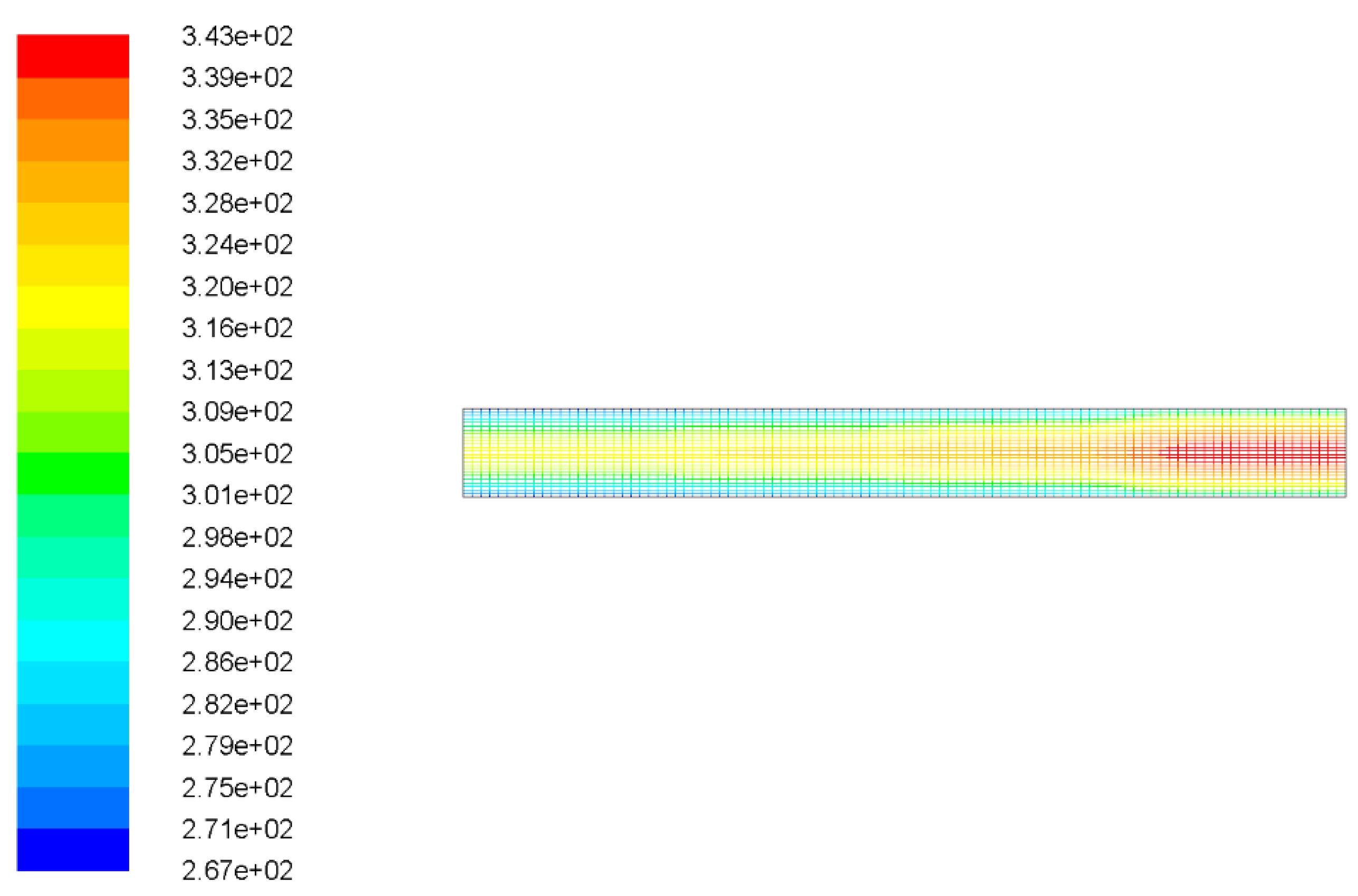
Figure 18.
Upper shell structure of NACA 0012 airfoil.
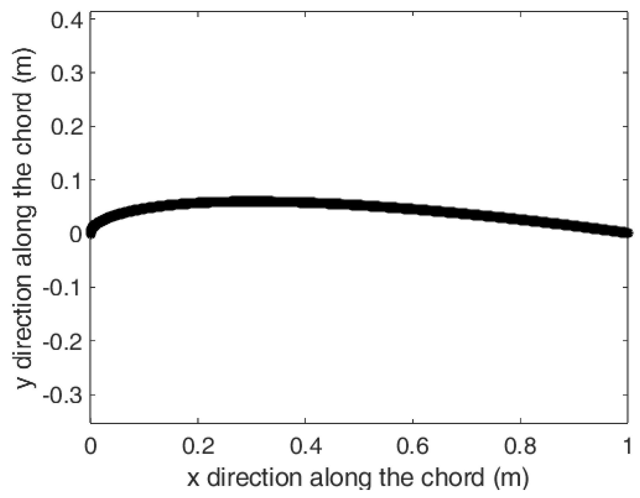
Figure 19.
Temperature contours on 0.001 m thick NACA 0012 airfoil upper shell structure at qgen=2E6 W/m3.
Figure 19.
Temperature contours on 0.001 m thick NACA 0012 airfoil upper shell structure at qgen=2E6 W/m3.
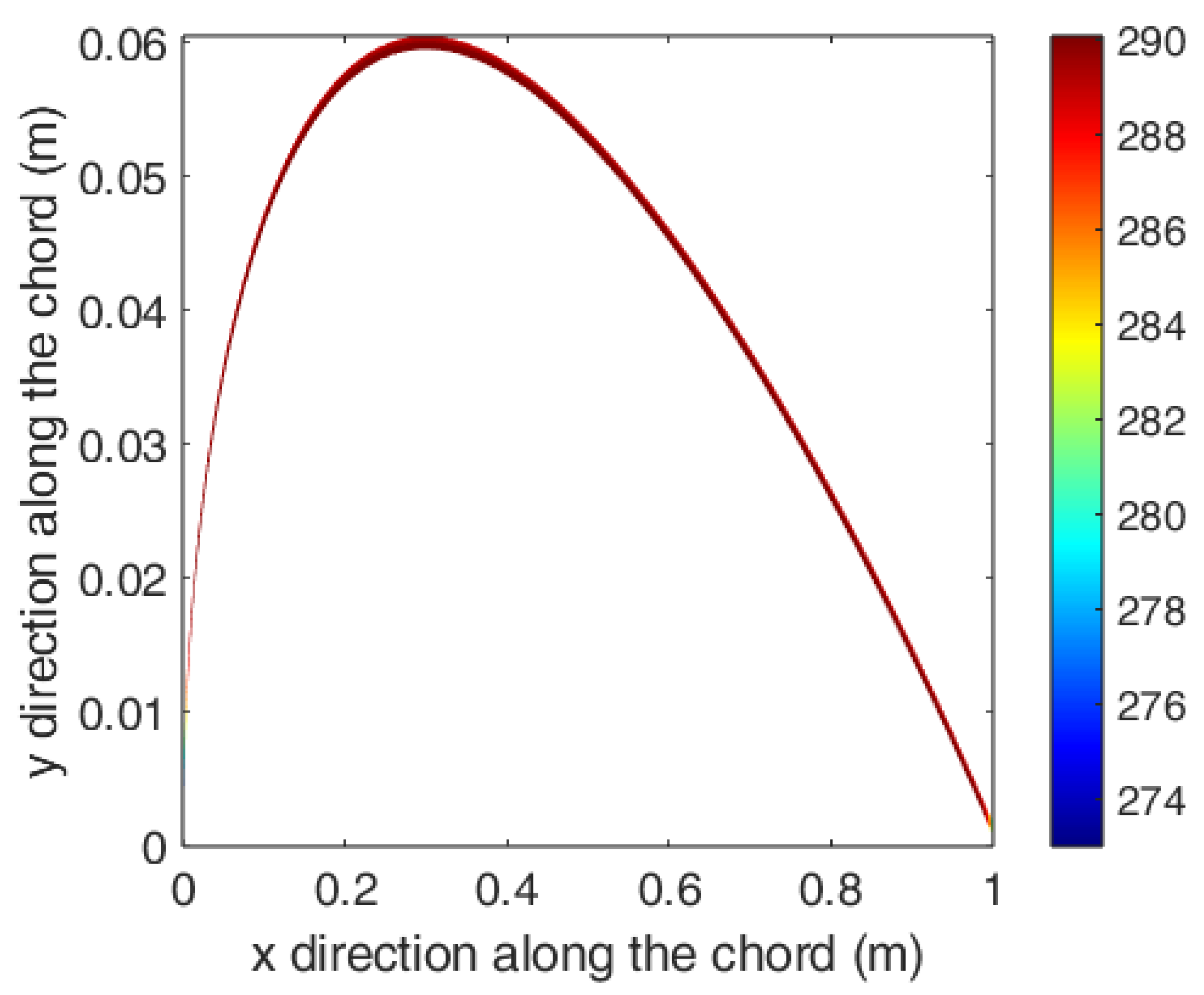
Figure 20.
Temperature contours on 1 m x 0.001 m rectangular plate at qgen=2E6 W/m3.
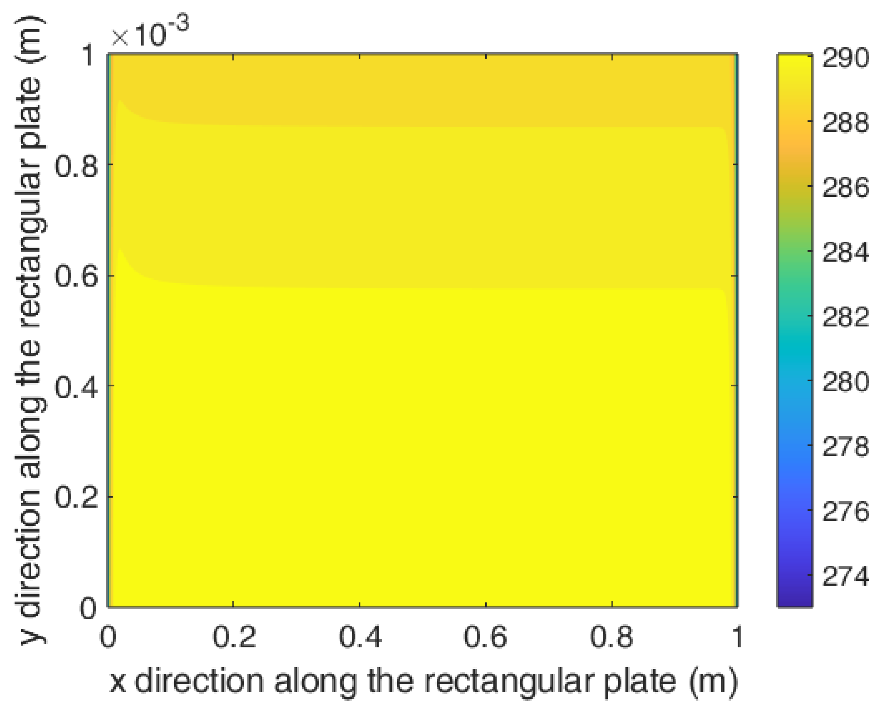
Figure 21.
Temperature contours on 0.001 m thick NACA 0012 airfoil upper shell structure at qgen=2.5E6 W/m3.
Figure 21.
Temperature contours on 0.001 m thick NACA 0012 airfoil upper shell structure at qgen=2.5E6 W/m3.
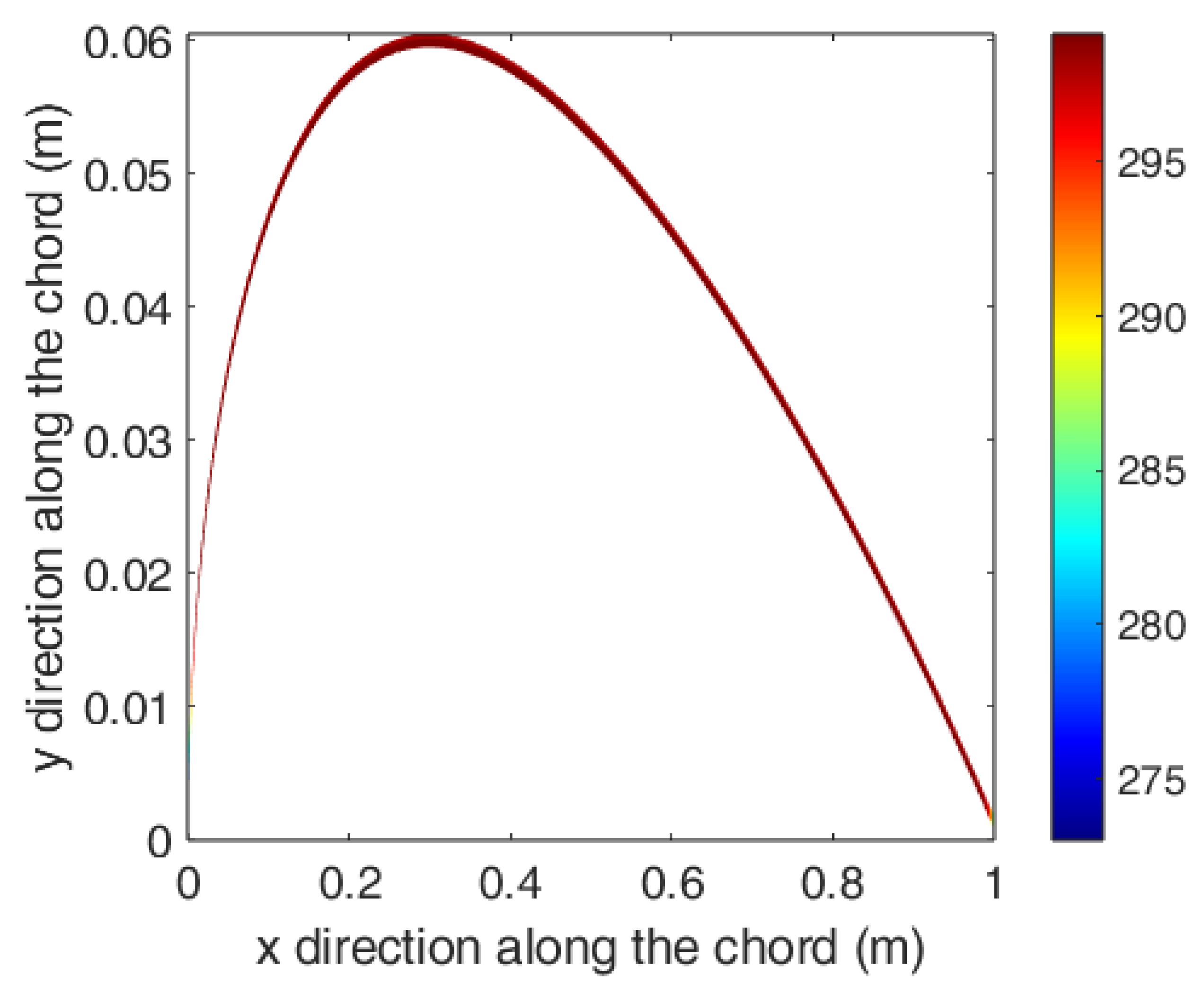
Figure 22.
Temperature contours on 1 m x 0.001 m rectangular plate at qgen=2.5E6 W/m3.
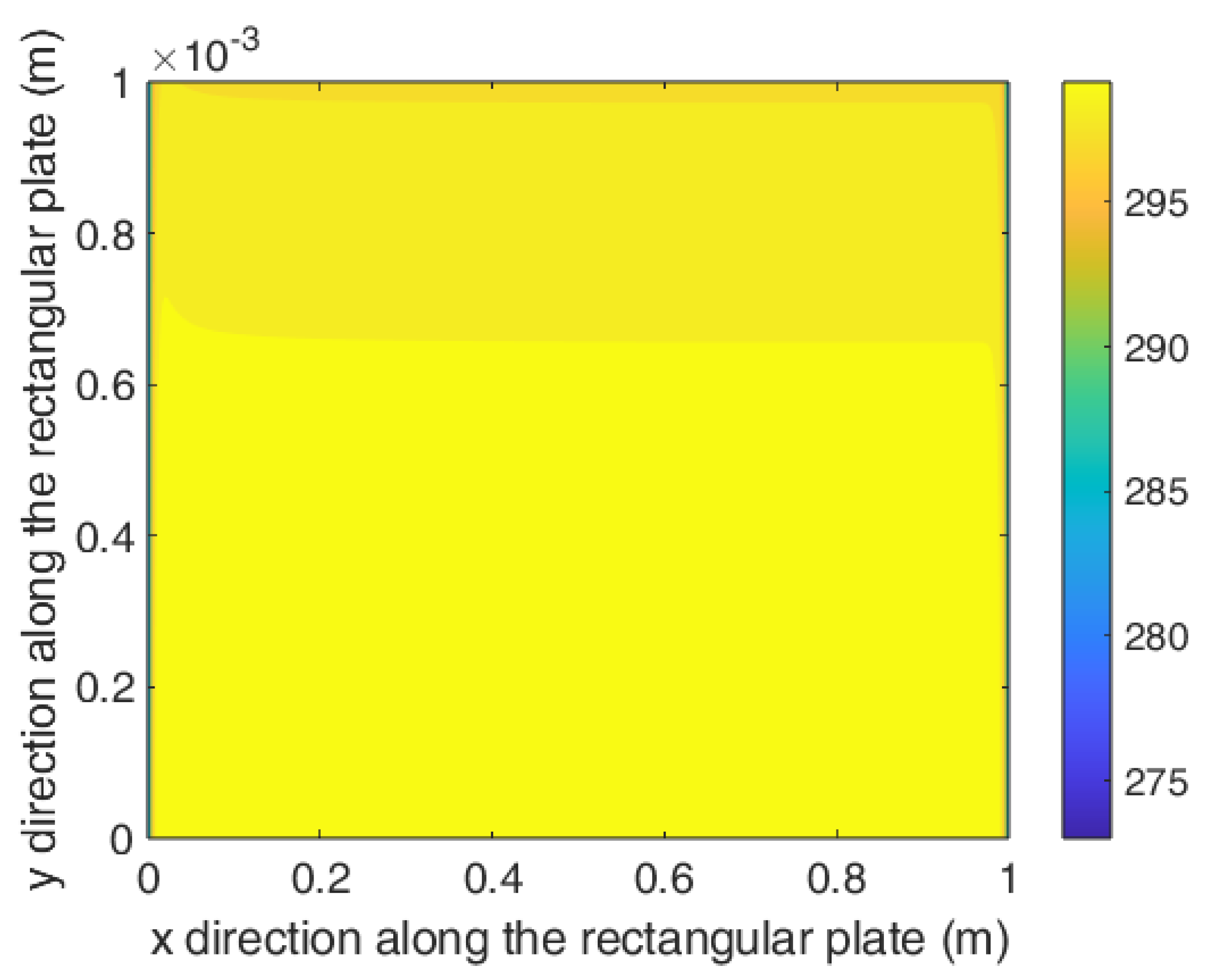
Figure 23.
Temperature contours on 0.001 m thick NACA 0012 airfoil upper shell structure at qgen=3E6 W/m3.
Figure 23.
Temperature contours on 0.001 m thick NACA 0012 airfoil upper shell structure at qgen=3E6 W/m3.
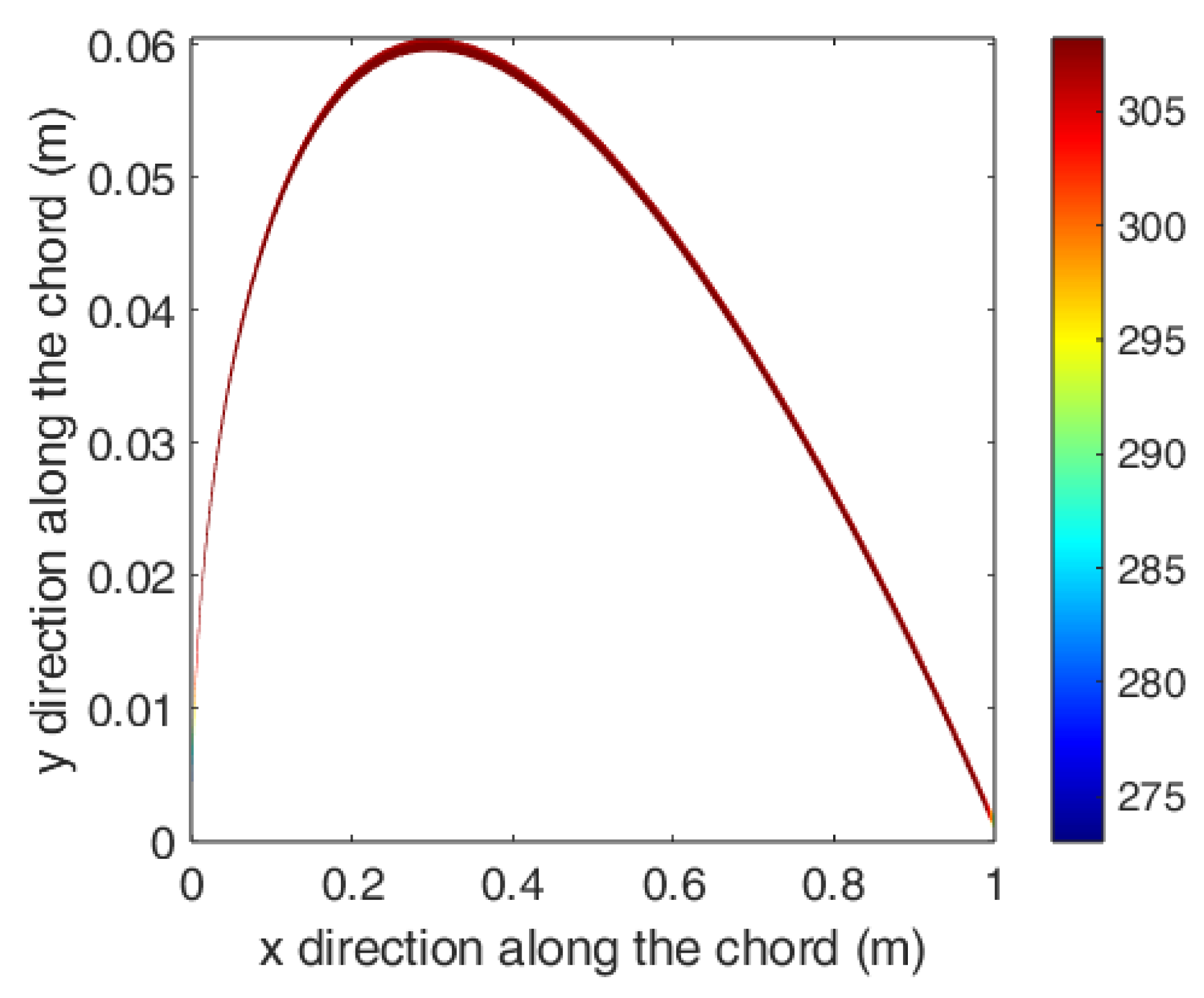
Figure 24.
Temperature contours on 1 m x 0.001 m rectangular plate at qgen=3E6 W/m3.
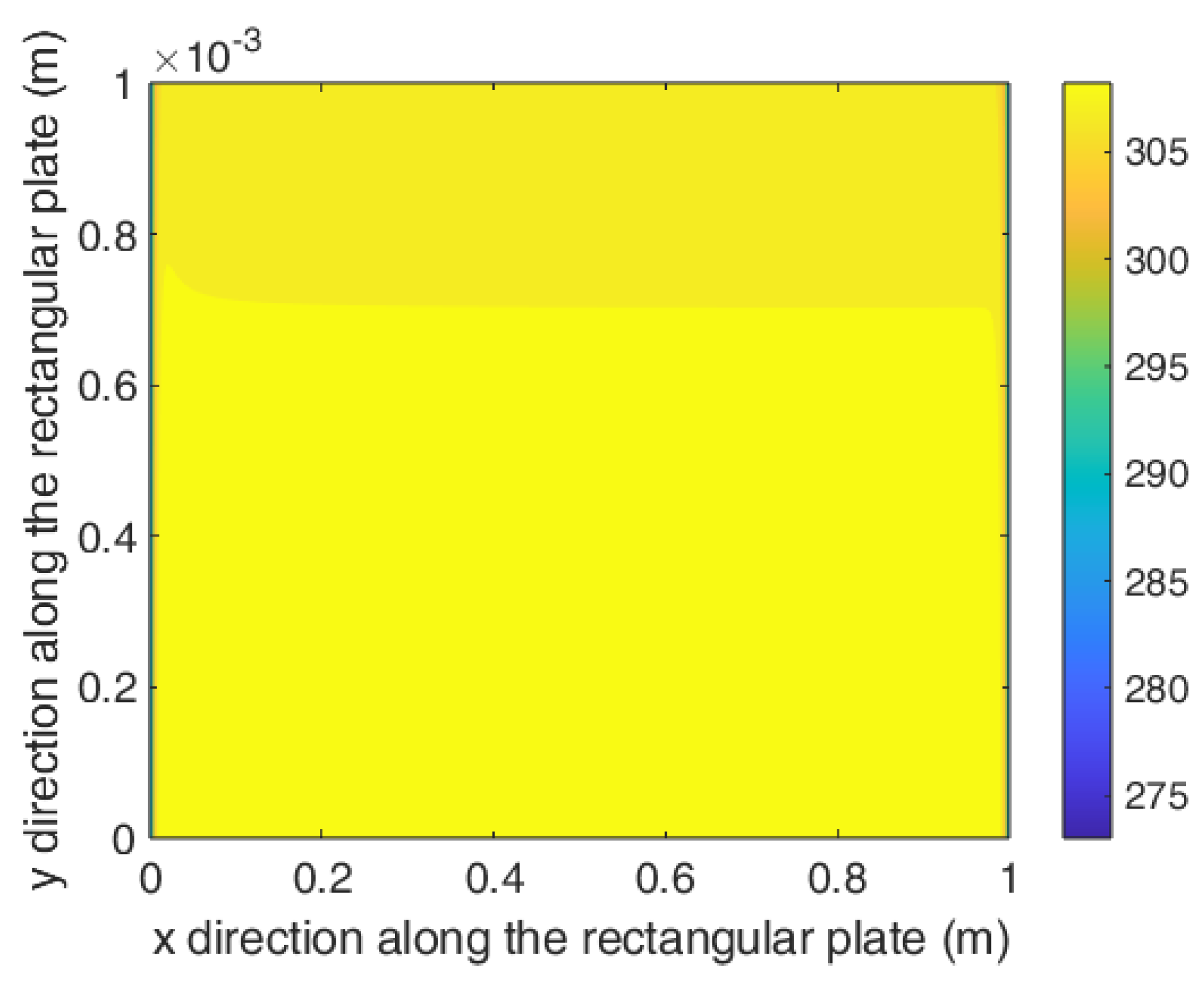
Figure 25.
Summary of the optimization procedure based on the genetic algorithm.
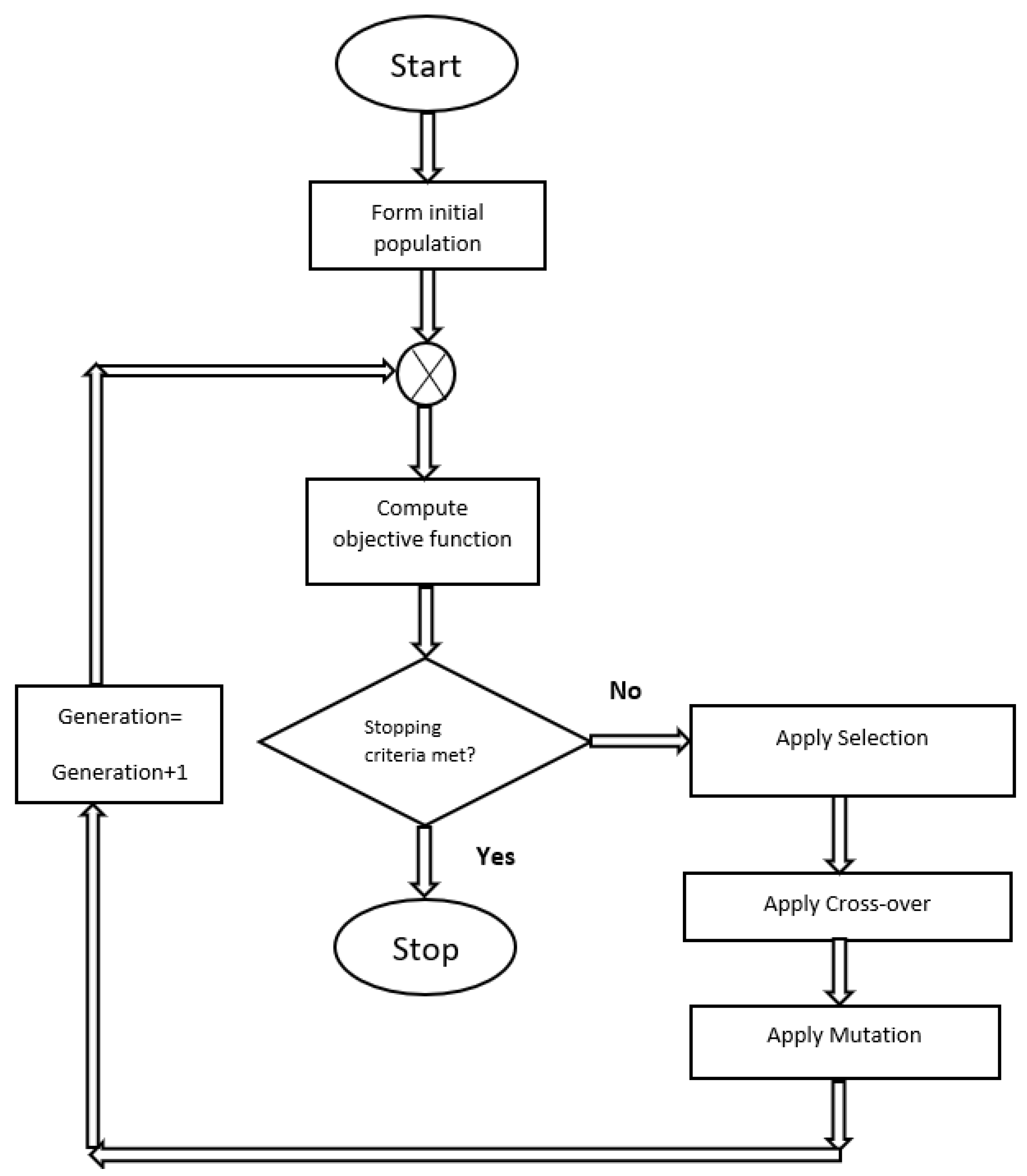
Figure 26.
Comparison of convective heat transfer coefficient distributions obtained from the genetic-algorithm-based correlation and RANS simulations at Re=9.4×10⁵ for NACA 0012 airfoil.
Figure 26.
Comparison of convective heat transfer coefficient distributions obtained from the genetic-algorithm-based correlation and RANS simulations at Re=9.4×10⁵ for NACA 0012 airfoil.
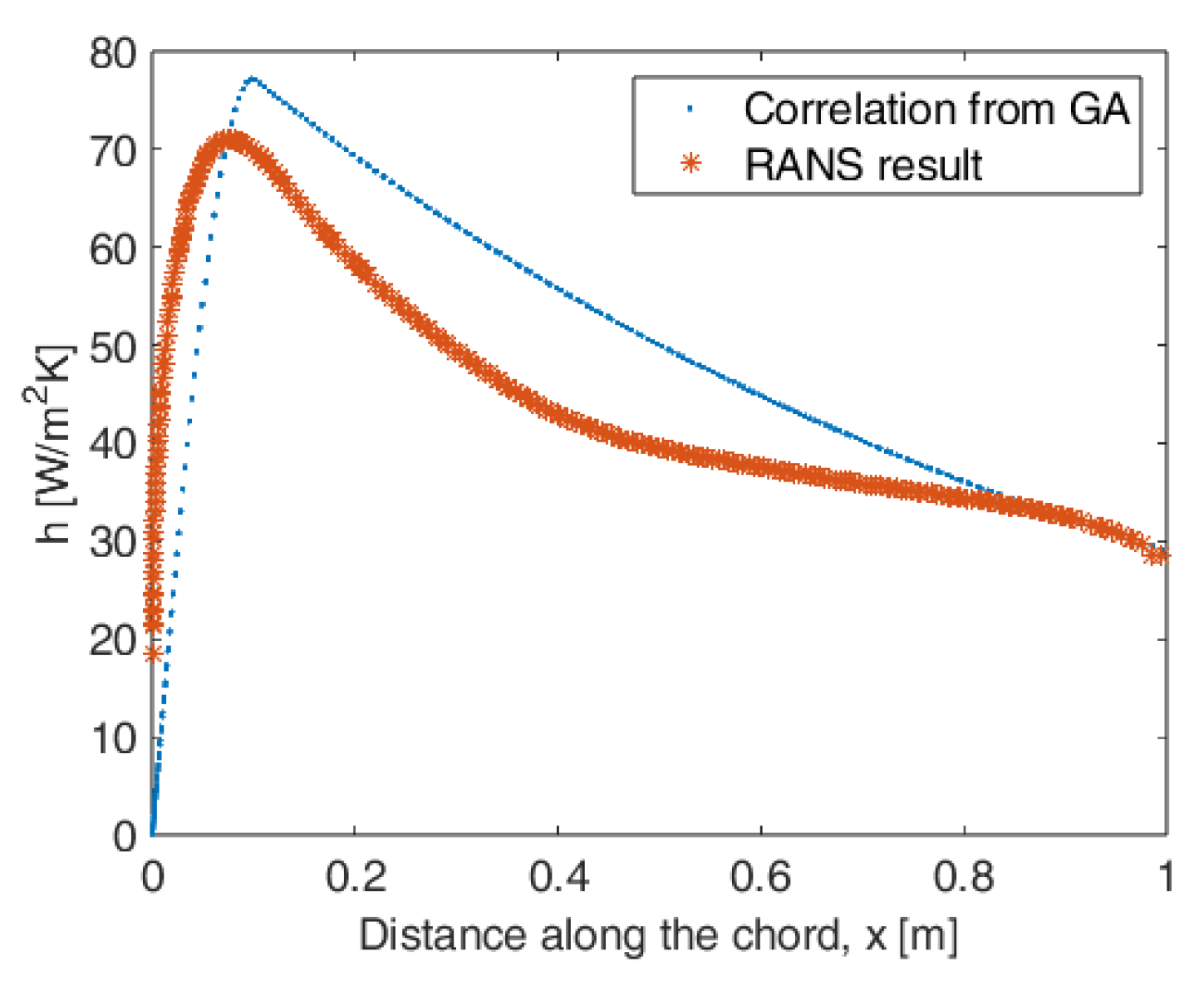
Figure 27.
Comparison of convective heat transfer coefficient distributions obtained from the genetic-algorithm-based correlation and RANS simulations at Re=1.88×10⁶ for NACA 0012 airfoil.
Figure 27.
Comparison of convective heat transfer coefficient distributions obtained from the genetic-algorithm-based correlation and RANS simulations at Re=1.88×10⁶ for NACA 0012 airfoil.
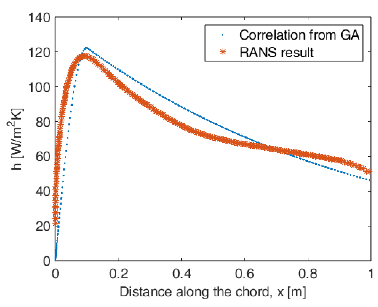
Figure 28.
Comparison of convective heat transfer coefficient distributions obtained from the genetic-algorithm-based correlation and RANS simulations at Re=3.12×10⁶ for NACA 0012 airfoil.
Figure 28.
Comparison of convective heat transfer coefficient distributions obtained from the genetic-algorithm-based correlation and RANS simulations at Re=3.12×10⁶ for NACA 0012 airfoil.
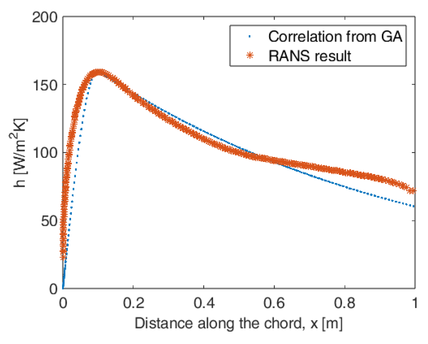
Figure 29.
Comparison of convective heat transfer coefficient distributions obtained from the genetic-algorithm-based correlation and RANS simulations at Re=9.4×10⁵ for NACA 0015 airfoil.
Figure 29.
Comparison of convective heat transfer coefficient distributions obtained from the genetic-algorithm-based correlation and RANS simulations at Re=9.4×10⁵ for NACA 0015 airfoil.
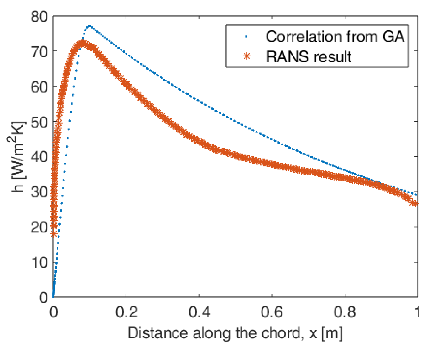
Figure 30.
Comparison of convective heat transfer coefficient distributions obtained from the genetic-algorithm-based correlation and RANS simulations at Re=1.88×10⁶ for NACA 0015 airfoil.
Figure 30.
Comparison of convective heat transfer coefficient distributions obtained from the genetic-algorithm-based correlation and RANS simulations at Re=1.88×10⁶ for NACA 0015 airfoil.
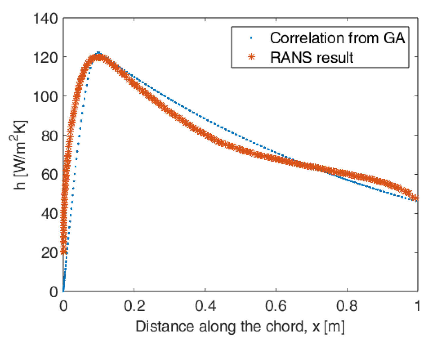
Figure 31.
Comparison of convective heat transfer coefficient distributions obtained from the genetic-algorithm-based correlation and RANS simulations at Re=3.12×10⁶ for NACA 0015 airfoil.
Figure 31.
Comparison of convective heat transfer coefficient distributions obtained from the genetic-algorithm-based correlation and RANS simulations at Re=3.12×10⁶ for NACA 0015 airfoil.
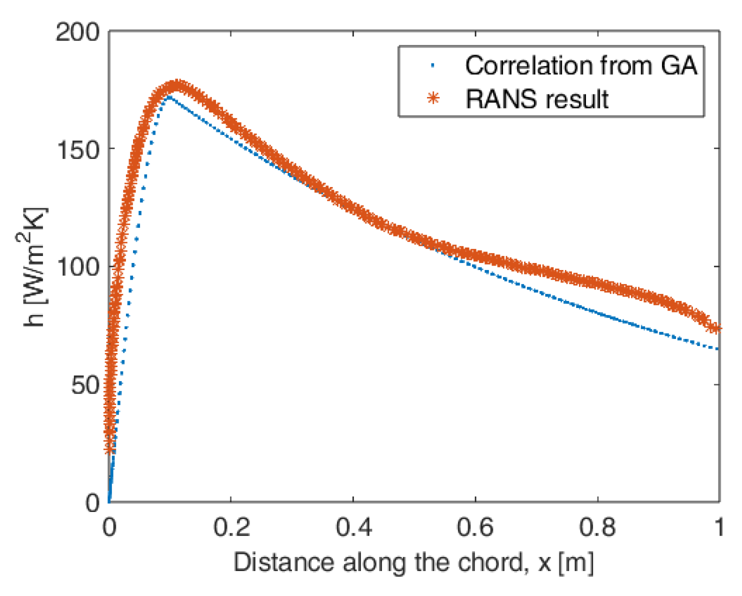
Figure 32.
Comparison of convective heat transfer coefficient distributions obtained from the genetic-algorithm-based correlation and RANS simulations at Re=9.4×10⁵ for NACA 0018 airfoil.
Figure 32.
Comparison of convective heat transfer coefficient distributions obtained from the genetic-algorithm-based correlation and RANS simulations at Re=9.4×10⁵ for NACA 0018 airfoil.
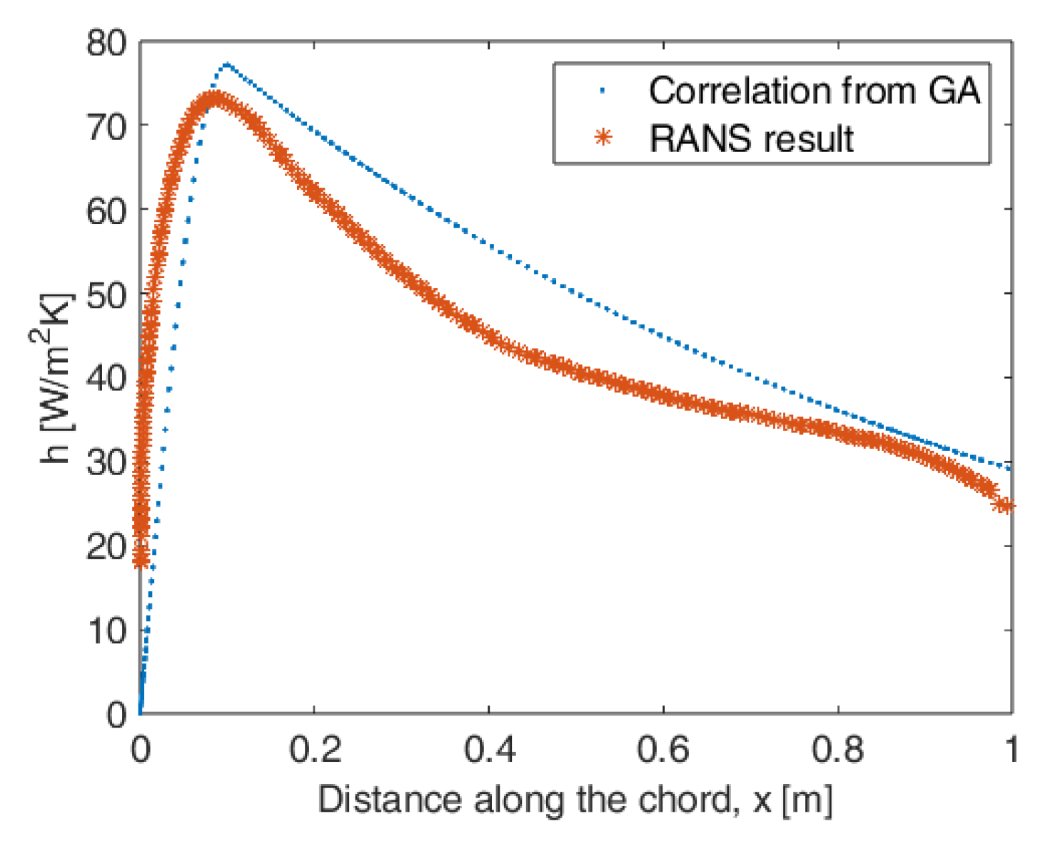
Figure 33.
Comparison of convective heat transfer coefficient distributions obtained from the genetic-algorithm-based correlation and RANS simulations at Re=1.88×10⁶ for NACA 0018 airfoil.
Figure 33.
Comparison of convective heat transfer coefficient distributions obtained from the genetic-algorithm-based correlation and RANS simulations at Re=1.88×10⁶ for NACA 0018 airfoil.
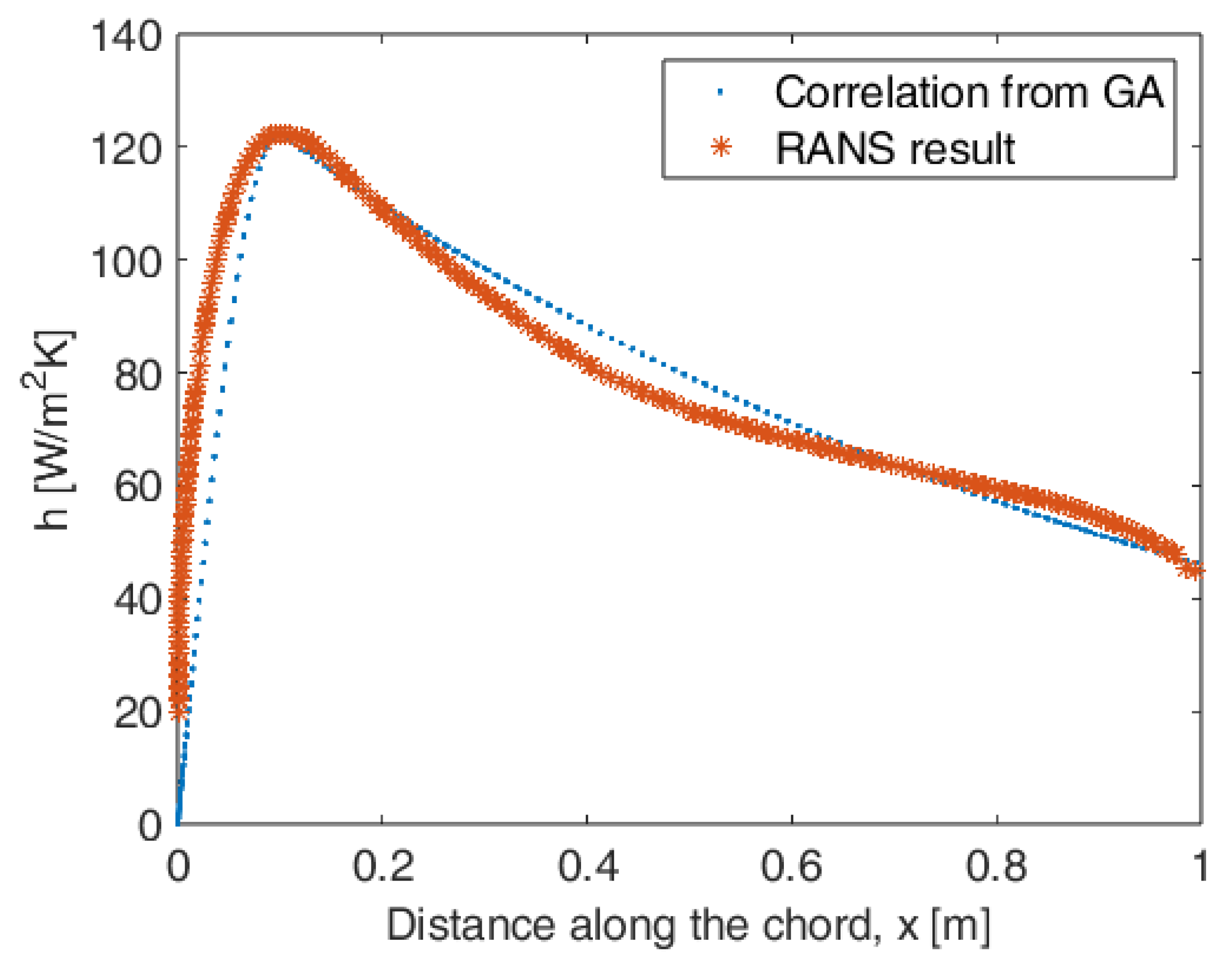
Figure 34.
Comparison of convective heat transfer coefficient distributions obtained from the genetic-algorithm-based correlation and RANS simulations at Re=3.12×10⁶ for NACA 0018 airfoil.
Figure 34.
Comparison of convective heat transfer coefficient distributions obtained from the genetic-algorithm-based correlation and RANS simulations at Re=3.12×10⁶ for NACA 0018 airfoil.
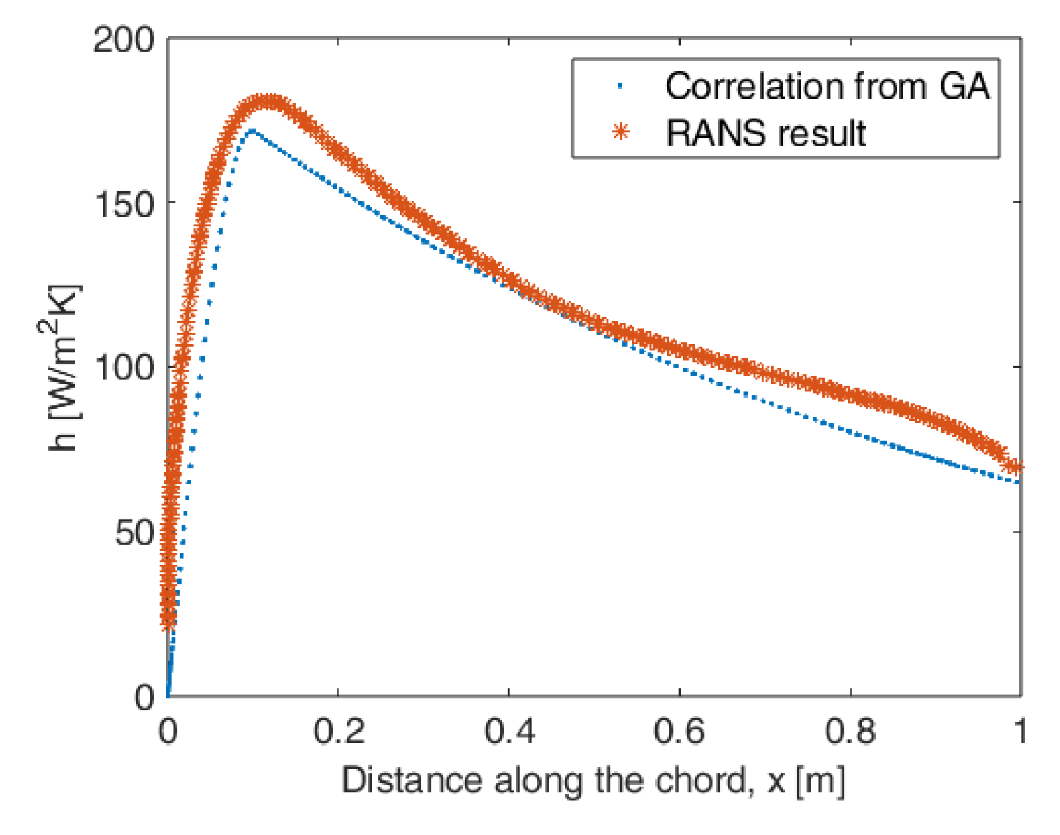
Figure 35.
Convergence plot of the optimization study for h equation development.
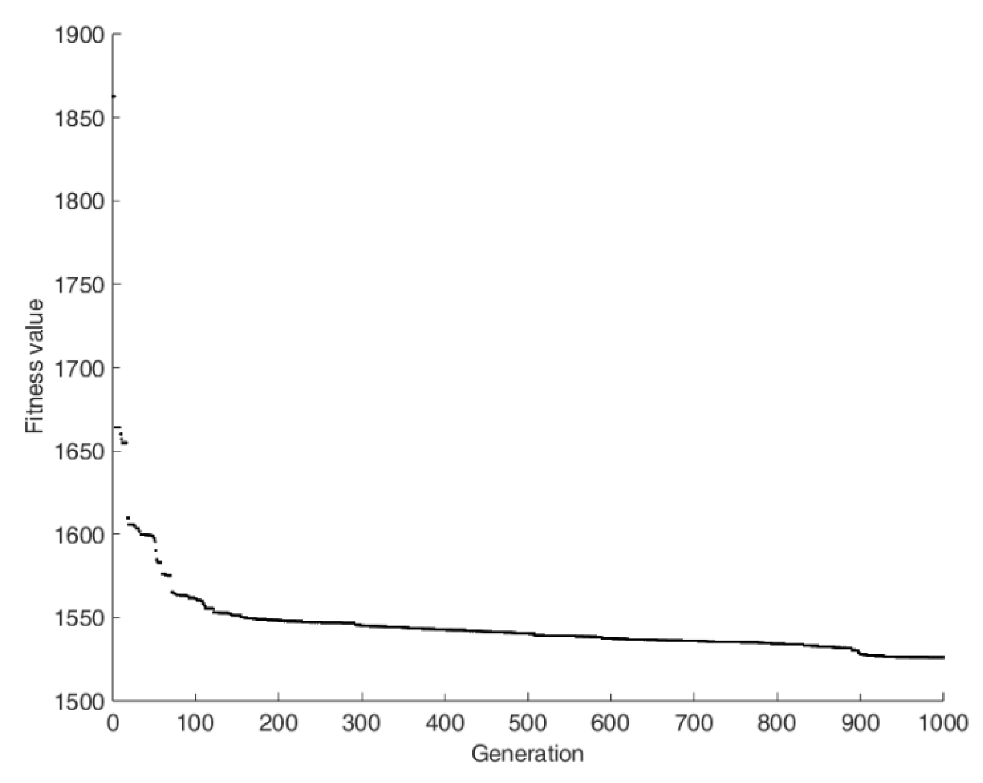
Figure 36.
Convergence plot for the second optimization study.
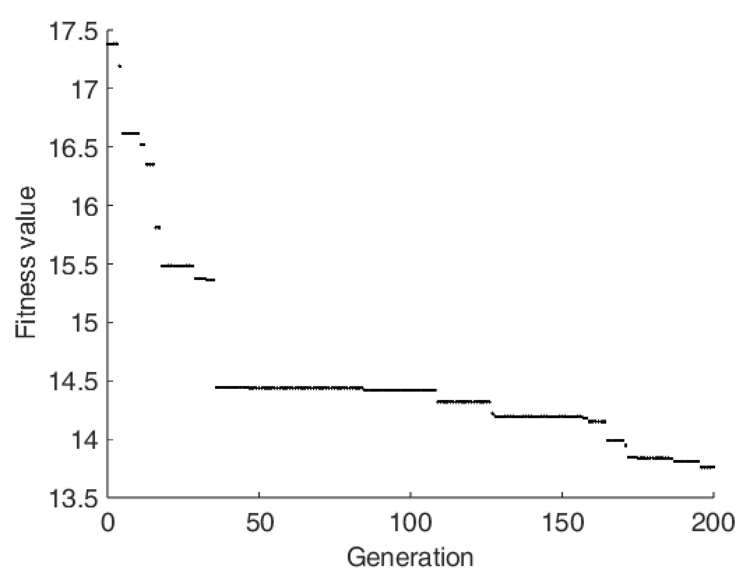
Figure 37.
Temperature isolines for the optimized electrothermal heating configuration under variable convective heat transfer coefficient.
Figure 37.
Temperature isolines for the optimized electrothermal heating configuration under variable convective heat transfer coefficient.
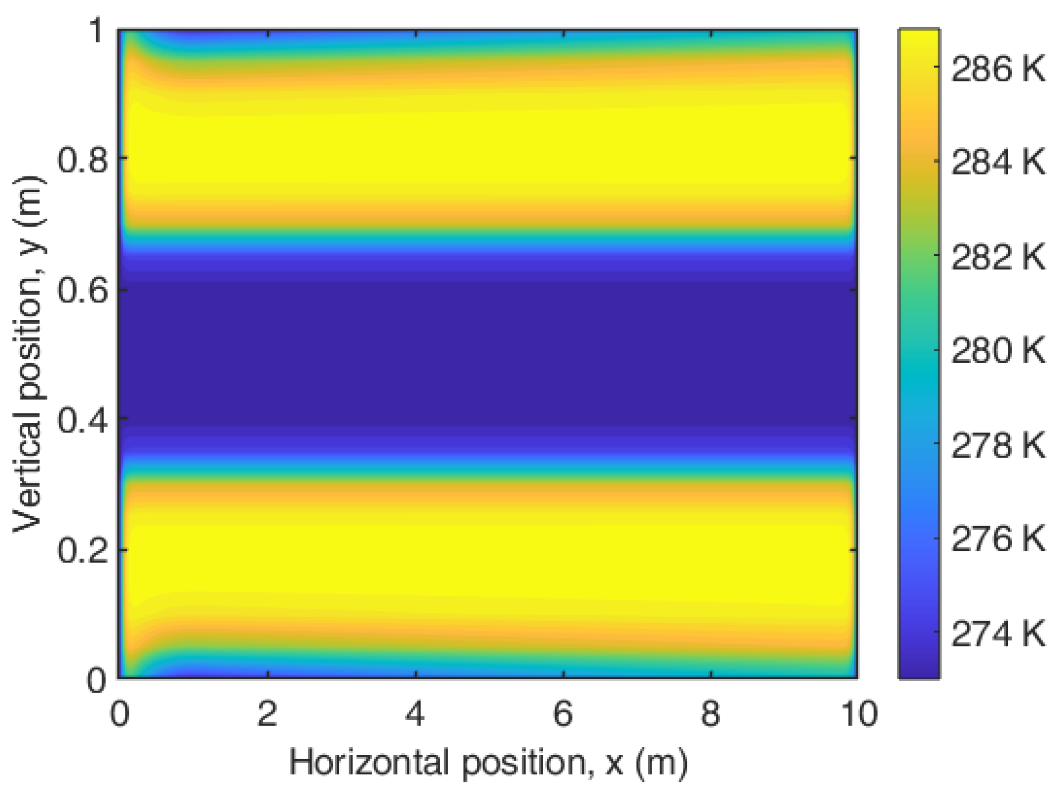
Figure 38.
Temperature isolines for the optimized electrothermal heating configuration under variable convective heat transfer coefficient with ply orientation variable included in the optimization.
Figure 38.
Temperature isolines for the optimized electrothermal heating configuration under variable convective heat transfer coefficient with ply orientation variable included in the optimization.
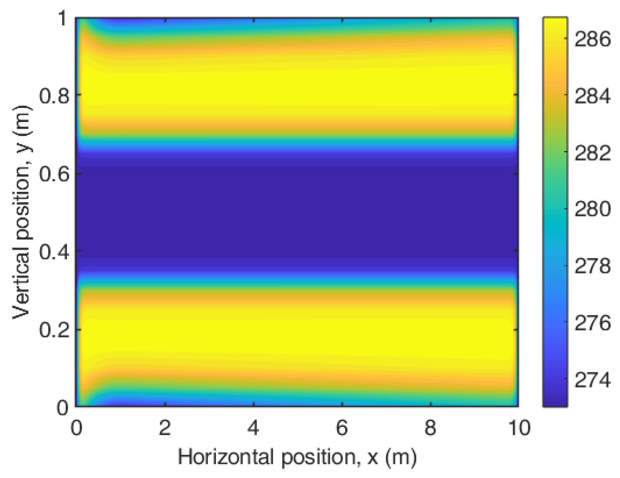
Figure 39.
Convergence plot for the third optimization study.
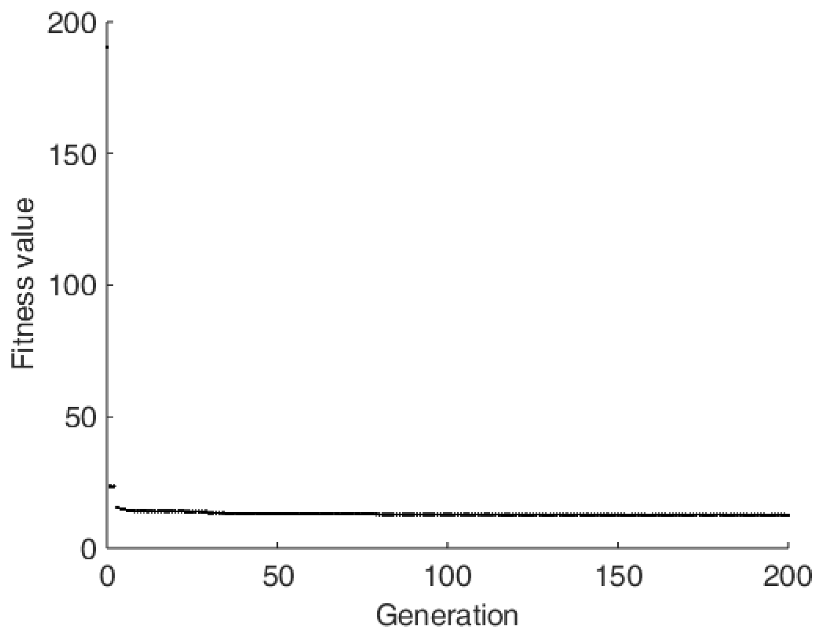
Figure 40.
Temperature (K) distribution of the optimized configuration, optimization study 4.
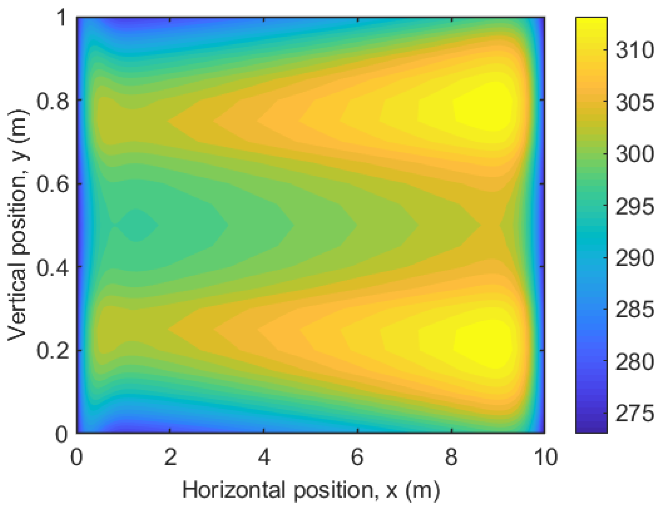
Figure 41.
Convergence plot for the fourth optimization study.
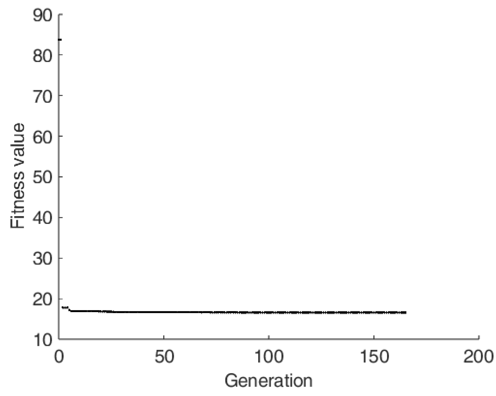

Table 1.
Optimized design parameters obtained from the genetic algorithm.
| Variable name | Heat generation rate | Width of Heater band | kx value for the composite | k value for the surface material |
| Result | 12715 (W/m3) | 25 cm | 0.6(W/m.K) | 10 (W/m.K) |
Table 2.
Sensitivity analysis of the optimized electrothermal heating configuration. held constant. Objective function variations are reported relative to the optimized baseline solution. The heater band width was perturbed according to the discrete integer-mapped transformation strategy used in the optimization framework.
| Design Variable | Perturbed and Optimum Values | Surface Temperature at the Half-Length (K) |
| Volumetric heat generation rate | +10%0-10% | 282.55 280.97 278.27 |
| Composite in-plane thermal conductivity | +10%0-10% | 279.63 280.97 279.59 |
| Surface material thermal conductivity | +10%0-10% | 280.47 280.97 278.64 |
Table 3.
Optimized design parameters obtained from the genetic algorithm.
| Variable name | Heat generation rate | Width of Heater band | Orientation of the plies | k value for the surface material |
| Result | 11653 (W/m3) | 25 cm | 0 (deg) | 10 (W/m.K) |
Table 4.
Optimized design parameters obtained from the Optimization Study 4.
| Heat generation rate (W/m3) | Ply 1 orientation (deg) | Ply 2 orientation (deg) | Ply 3 orientation (deg) | Surface coating thermal conductivity (W/m.K) |
| 2070 | 0 | 45 | 0 | 10 |
Disclaimer/Publisher’s Note: The statements, opinions and data contained in all publications are solely those of the individual author(s) and contributor(s) and not of MDPI and/or the editor(s). MDPI and/or the editor(s) disclaim responsibility for any injury to people or property resulting from any ideas, methods, instructions or products referred to in the content. |
© 2026 by the authors. Licensee MDPI, Basel, Switzerland. This article is an open access article distributed under the terms and conditions of the Creative Commons Attribution (CC BY) license (http://creativecommons.org/licenses/by/4.0/).
Copyright: This open access article is published under a Creative Commons CC BY 4.0 license, which permit the free download, distribution, and reuse, provided that the author and preprint are cited in any reuse.


