
Submitted:
04 January 2026
Posted:
05 January 2026
You are already at the latest version
Abstract
Atmospheric rivers (ARs) play a critical role in producing high-impact weather events including extreme precipitation, flooding, gusty winds, and rapid temperature changes. Building upon the recently published EDARA (ERA5-based Dataset for Atmospheric River Analysis), we present S-EDARA, a supplementary dataset that enhances AR impact assessment capabilities through a newer AR detection algorithm and additional impact-related metrics. S-EDARA includes AR shapes identified by the tARget version 4 (ARS4) algorithm, strong integrated vapour transport (SIVT) indicators, and pseudo total precipitation rate (PTPR) fields. The dataset features both numerical data and interactive graphical catalogues displaying ARS4, SIVT, PTPR, gusty winds, and 24-hour temperature changes at 6-hourly intervals. These enhancements enable more comprehensive analysis of AR impacts and characteristics, particularly for regions experiencing rapidly changing meteorological conditions during AR events. The dataset covers the period from 1940 to present and is publicly available through the Federated Research Data Repository.
Keywords:
atmospheric river
; ERA5 reanalysis
; EDARA
; tARget algorithms
; water vapour transport
; flooding
; landslides
; Chinook events
; Foehn events
1. Background and Summary
Atmospheric Rivers (ARs) are narrow bands of strong horizontal water vapour transport concentrated in the lower troposphere that can trigger high-impact weather including extreme precipitation, flooding, damaging winds, and temperature anomalies [4,5,6,7,8,9,10,11,12,13]. To put this in a historical perspective, Figure 1 depicts a moisture-laden AR triggering multiple high-impact weather events across western North America in November 1962. This storm dropped 100 to 200 mm of precipitation over southwestern Washington, USA during 19–21 November; with freezing level rising to about 3000 metres, runoff from melting snow and heavy precipitation caused river streams to rise rapidly and led to flooding in many of the lower valleys [14,15]. It also brought hurricane-force winds, heavy rain and melting snow to southwestern British Columbia, Canada, causing flooding, power outages, and an estimated $100,000 of highway damage [16]. Furthermore, this AR extended its influence beyond the Coast Mountain Range, causing an extreme Chinook event on the leeside of the Rocky Mountains with gusty winds and rapid temperature rising across the Canadian Prairies (Figure 1c,d); a maximum gust of 171 km/h was recorded at Lethbridge Airport in Alberta, Canada [17].
The original EDARA (ERA5-based Dataset for Atmospheric River Analysis) [2,3] provides a comprehensive foundation for AR analysis, containing 12 meteorological variables derived from ERA5 reanalysis [18] and graphical AR catalogues based on the tARget version 3 (tARget-v3) algorithm. However, continued development of AR detection methodologies and growing interest in AR impacts necessitate expanded datasets to support evolving research needs. In particular, the tARget algorithm has been continually refined, with version 4 (tARget-v4) incorporating improvements to better handle ARs in tropical and polar areas, as well as “zonal” ARs which previous versions were not designed to capture [19]. This latest version provides enhanced global coverage and more robust AR identification across diverse geographical regions and atmospheric conditions.
As a supplement to EDARA, S-EDARA addresses two key limitations of the original dataset: (1) it incorporates the latest tARget-v4 detection algorithm for improved AR identification, and (2) it includes additional impact-relevant variables that facilitate assessment of AR-related hazards. The supplementary dataset is specifically designed to enable researchers to:
- Compare AR detection outcomes between tARget-v3 and tARget-v4 algorithms
- Identify regions experiencing anomalously strong moisture transport through SIVT (Strong Integrated Vapour Transport)
- Assess AR-related precipitation potential through PTPR (Pseudo Total Precipitation Rate)
- Analyse concurrent wind and temperature extremes associated with AR events
- Validate detection algorithms through Feature Occurrence Frequency (FOF) metrics
This supplementary dataset maintains EDARA’s temporal resolution (6-hourly) and spatial coverage (global) while adding new variables and visualization capabilities that enhance understanding of AR impacts.
2. Methods
2.1. Data Sources
All S-EDARA and EDARA variables are derived from the European Centre for Medium-Range Weather Forecasts (ECMWF) ERA5 atmospheric reanalysis. As a comprehensive, high-resolution global climate dataset, ERA5 provides hourly atmospheric data 0.25° × 0.25° horizontal resolution from 1940 to near real-time [18]. It combines model forecasts with vast observational data to create a consistent historical record for climate research, model validation, and understanding climate change. For consistency with EDARA, S-EDARA processes ERA5 data at 6-hourly intervals (0000, 0600, 1200, and 1800 UTC).
2.2. Integrated Vapour Transport (IVT)
As in EDARA, the AR detection is based on the distribution and climatology of the IVT, which is calculated by vertically integrating the product of the specific humidity and the horizontal wind from the Earth surface to a specified pressure level in the upper troposphere:
where is a two-dimension vector called the Integrated Vapour Flux (IVF), is the gravitational acceleration, is the air density, is the upward distance from the Earth surface, and is the air pressure; the vertical coordinate transformation in the above equation is based on the hydrostatic equation . The integration limits and denote pressures at the top () and the base () of the air column, respectively. For both EDARA and S-EDARA, we chose hPa and , where represents the variable surface pressure. Note that hPa [4,6,20] or hPa [21] were also chosen in some AR studies. Given that decreases rapidly with height, changing within the range of 100-300 hPa has a negligibly small contribution to IVT [22]. On the other hand, more noticeable discrepancies may arise between the choices of hPa and , given that could be much lower than 1000 hPa over complex terrain. A python script designed to handle was provided in EDARA [2].
2.3. Relationship Between Precipitation and Water Vapour Transport
From a water balance perspective, the local change of water content in the atmosphere can only occur through the addition or subtraction in any of its three possible phases (vapour, liquid, and solid), as described by the following balance equation [22,23]:
where is the vertical velocity in the coordinate system, is the averaged vertical velocity of the condensed water (liquid droplets or solid ice particles) relative to air, and represents the two-dimensional horizontal divergence operator. Vertically integrating this equation from the Earth’s surface () to the top of the air column () and assuming at the top (), we obtain
with being the liquid water density, the precipitation rate and the evapotranspiration rate, both measured at the Earth’s surface, and
In the above equations, represents the combined process of water vapour moving into the base of air column, through evaporation from surfaces and transpiration from plants; represents the downward condensed phase flux measured at the Earth’s surface; W and are the integrated water vapour and the integrated condensed water, respectively; is the total condensed water transport due to clouds passing through the atmosphere. The quantities and represent the rates of change in condensed phase and in vapour stage of water storage with the air column, respectively. The inclusion of in Equation (3) implies that P and E are measured in terms of height of equivalent water per unit time, such as or .
Equation (3) indicates that precipitation (P) is associated with net convergence of water vapour flux () rather than with the IVT value [22,24]. For heavy precipitation events, such as those triggered by strong ARs, the dominant contribution to the precipitation process comes from the moisture convergence term on the right-hand side of Equation (3), , which results in general moistening and condensation within the air column. In S-EDARA, this term is called the Pseudo Total Precipitation Rate (PTPR), which is specifically defined as:
where the value of is rearranged as and is measured in . Multiplying by a factor of 3600 in the above equation changes the unit of PTPR from mm to , which is a more convenient unit for precipitation rate. A positive value of PTPR indicates moisture convergence and potential precipitation. It can be considered as the potential precipitation rate contributed from the horizontal water vapour transport process. This dynamical precipitation proxy complements direct precipitation observations and helps identify regions where AR-related moisture convergence drives precipitation generation.
For the North Pacific AR at 0000 UTC 20 November 1962, Figure 2 shows that the PTPR distribution is very similar and comparable to the total precipitation rate (TPR) distribution in Figure 1b. the PTPR distribution associated with the same AR event is plotted in Figure 2. In general, it can be expected that PTPR TPR because a fraction of the water vapour amount converged into an unsaturated air column contributes to moistening the atmosphere (leading to ) rather than condensing into precipitation [22].
2.4. Atmospheric River Detection with the tARget-v4 Algorithm
The tARget algorithm is a geometric approach to AR identification that defines these features based on integrated vapour transport (IVT) characteristics [19,25,26,27]. The tARget-v4 algorithm represents the latest update to the methodology, incorporating refinements in AR shape detection and boundary delineation compared to version 3 used in the original EDARA dataset. It applies the following requirements for AR detection [19]:
- (1)
- IVT Threshold. IVT objects are extracted based on the IVT value exceeding the location- and season-dependent 85th percentile threshold of local climatology. This adaptive threshold accounts for regional and seasonal variability in background moisture transport. For EDARA and S-EDARA, the 1991-2020 30-year climatology is used. To facilitate AR identification in cold and/or dry regions where IVT is climatologically low, an additional, location-independent IVT threshold is applied hemispherically, which raises the pixel-wise threshold to higher percentiles over 5% of the surface area of the corresponding hemisphere where IVT is climatologically the lowest. In previous tARget versions, a fixed lower limit of 100 for IVT was used to serve a similar purpose.
- (2)
-
Coherence and Geometry. Contiguous regions exceeding the IVT threshold must satisfy specific geometric constraints:
- The standard deviation of IVT directions across individual pixels ≤ 67.5° (to eliminate features closely associated with tropical cyclones).
- The axis of an IVT object having a contiguous segment (or multiple) segments totalling longer than 1000 km where each pixel has a poleward IVT component greater than 25% of the total IVT at that pixel (to remove features with entirely zonally-directed or equatorward IVT primarily found in the tropics).
- Minimum length of 2000 km and length-to-width ratio ≥2, calculated along the feature’s orientation axis.
- (3)
- Additional Iterations. If an IVT object fails the geometrical and directional requirements in the above steps, it is subject to additional iterations of these steps with each round the pixel-wise IVT threshold being raised by 2.5th percentile, up until the threshold reaches the 95th percentile.
- (4)
- Enhanced Extratropical Refinement. tARget-v4 introduces improved geometric requirements that better capture ARs in regions with complex topography and varying background flow patterns. The refinement reduces false positives in tropical regions while maintaining detection sensitivity in mid-to-high latitudes.
The tARget-v4 algorithm incorporates several refinements compared to tARget-v3 used in the original EDARA. These improvements result in a catalogue that more accurately represents AR distributions, particularly in regions of complex topography and high impact potential. The detected ARs at each time step are stored as a binary field (ARS4) in S-EDARA with grid points where ARs are present being assigned a value of 1 and all other points are assigned a value of 0.
2.5. Strong Integrated Vapour Transport (SIVT)
The tARget-v4 algorithm assumes that ARs are associated with strong IVT values and uses the IVT 85th percentile () as the starting threshold for AR identification. To identify regions where , we included a strong IVT (SIVT) field as a supplementary variable in S-EDARA, defined as
This threshold-based approach identifies regions experiencing anomalously high moisture transport relative to local climatology, which is relevant for impact assessment as these regions are more likely to experience extreme precipitation and flooding. Some further constraints must be satisfied for the tARget-v4 algorithm to identify the AR objects (ARS4 = 1) over the areas with SIVT = 1.
2.6. Graphical Atmospheric River Catalogues
S-EDARA also includes a graphical catalogue for each month to support comprehensive high-impact weather assessment. This tool allows visualising the tARget-v4-based AR features and their potential impacts through a web browser, as shown in Figure 3.
Users can use the forward and backward buttons to go through different time steps at 6-hour intervals. There are four panels for each time step. The blue solid lines in (a), (c), and (d) mark the boundaries of ARs (i.e., ARS4 = 1), and those in (b) mark the boundaries of SIVT = 1. The IVT and IVF distributions are shown in (a). The PTPR distribution is plotted in (b), which can be compared to the TPR distribution provided in the corresponding EDARA catalogue. Additional impact variables plotted in (c) and (d) are:
- Change of Temperature in 24 hours at 2 metres above ground (CT24h). It is computed as , where represents 2-metre air temperature (Figure 3d).
2.7. Data Format and Structure
S-EDARA numerical data are provided in netCDF format, following CF (Climate and Forecast) conventions for metadata. Each netCDF file includes three variables: ARS4, SIVT, and PTPR, with complete metadata describing variable definitions, units, and processing methods. Spatial coordinates follow standard latitude-longitude grids consistent with ERA5 and the original EDARA dataset. Temporal coordinates are provided in the ISO 8601 format (e.g., 1962-11-20T00:00:00.000000000 for 0000 UTC 20 November 1962). Graphical catalogues are provided as PNG images showing spatial distributions of all variables (ARS4, SIVT, PTPR, gusty wind, and 24-hour temperature change) at selected time steps representing diverse AR events and geographic regions. These visualizations facilitate rapid assessment of AR characteristics and impacts without requiring specialized data processing tools.
2.8. Feature Occurrence Frequency
Feature Occurrence Frequency (FOF) is defined as a validation metric to quantify the spatial and temporal prevalence of a specified feature, such as ARS4 and SIVT. It is defined as:
where is the binary indicator for feature presence at location and time t, and N is the total number of time steps in the analysis period.
FOF expressed as a percentage (0-100%) represents the fraction of time a feature is present at each grid point, enabling:
- Identification of AR hotspots and primary tracks
- Validation against independent observations or alternative detection methods
- Assessment of algorithm sensitivity to detection criteria
3. Data Description
The S-EDARA dataset is deposited at the Federated Research Data Repository (FRDR, https://doi.org/10.20383/103.01528) [1] and consists of three components: numerical data files, graphical catalogues, and miscellaneous documents. It can be used in conjunction with the EDARA dataset available from FRDR at https://doi.org/10.1038/s41597-024-03679-1 [2].
3.1. Numerical Data Files
The S-EDARA data component consists of monthly netCDF files from January 1940 to near present. These data files can be found in the “data” folder, named in the form S_EDARA_yyyymm.nc (e.g., S_EDARA_202503.nc). In each file, 6-hourly (0000, 0600, 1200, 1800 UTC) data of three variables through the month are stored at a 0.25° global grid. These variables are listed and briefly described as follows.
- Atmospheric River Shapes (ARS4): Binary fields indicating the spatial extent of detected ARs based on the tARget-v4 algorithm.
- Strong Integrated Vapour Transport (SIVT): Binary fields identifying regions where IVT exceeds the local 85th percentile threshold.
- Pseudo Total Precipitation Rate (PTPR): Continuous fields of normalized integrated vapour convergence serving as a precipitation proxy. The unit of this variable is .
3.2. Graphical AR Catalogues
Monthly graphical catalogues can be accessed via any standard web browser in the “figs” folder. For each calendar month, there is a folder containing an HTML file named index.html and a subfolder “images” holding the image for each time step. Opening the index.html file with a browser brings up the catalogue interface (e.g., Figure 3) for visualising the global distributions of ARS4, IVT, and IVF in (a), SIVT and PTPR in (b), ARS4 and GWS10m in (c), and ARS4 and CT24h in (d), respectively.
3.3. Additional Program and Data Files
The README file in the top-level directory of S-EDARA provides detailed technical information to researchers about how to use this dataset. There are 10 additional program and data files located in the “misc” folder. They are included mainly for demonstration purposes.
- misc/Extract_variables_fromera5dara.py. This python program illustrates how to access data in a netCDF file downloaded from the EDARA database. Note that the EDARA variables Qu, Qv, GWS10m, and T2m are needed for creating the S-EDARA numerical data files and graphical catalogues. They were not re-created from ERA5 but directly extracted from EDARA. This program takes one data file as input and generates one output data file.
- misc/target.m. This is the tARget-v4 algorithm written in MATLAB. It was provided by Guan and Waliser [19], available via the Global Atmospheric Rivers Dataverse (https://dataverse.ucla.edu/dataverse/ar). This program takes three data files as inputs and generates an output data file.
- misc/Create_S_EDARA_data.py. This python program illustrates how to create a data file in netCDF format as those available in the data folder. It needs three input data files and generates one output data file.
- misc/era5dara_202503.nc. This is a data file needed as an input data file for the two python programs misc/Extract_variables_fromera5dara.py and misc/Create_S_EDARA_data.py. It was downloaded from the EDARA database.
- misc/ERA5_ivt_tARget_202503.nc. This is the output file from the python program misc/Extract_variables_fromera5dara.py. It contains the two IVF components and is used as one of the input files for the MATLAB program misc/target.m.
- misc/ERA5_islnd.nc. This is a data file constructed from the ERA5 land-sea mask. It is needed as one of the input files for the MATLAB program misc/target.m.
- misc/ERA5_monthly_pixel_ivt_limit.nc. This is a data file containing the monthly IVT percentile information based on a 30-year (1991-2020) climatology. It is needed as one of the input files for the MATLAB program misc/target.m. It is also used as an input file for the python program misc/Create_S_EDARA_data.py.
- misc/out_202503.nc. This is the output data file from the MATLAB program misc/target.m. It is also used as an input data file for the python program misc/Create_S_EDARA_data.py.
- misc/S_EDARA_202503.nc. This is the output data file from the python program misc/Create_S_EDARA_data.py.
- misc/About_S_EDARA.pdf. This document provides a brief description of the data and acronyms used in S-EDARA. It can be viewed by clicking the “About…” button in the graphical catalogue interface.
3.4. Data Volume, Download Options, and Updates
The complete S-EDARA dataset comprises approximately 125 GB of numerical data and 100 GB of graphical catalogues. The numerical data are compressed using netCDF-4 compression to reduce storage requirements while maintaining data integrity. The FRDR repository provides options for downloading the complete dataset or accessing individual months as needed for specific research applications.
As the ERA5 reanalysis continues to be updated with near-real-time data, S-EDARA will be periodically updated to maintain currency. Update frequency and version control information will be documented in the repository metadata. Users are encouraged to check the repository for the latest version and to cite the specific version used in their research.
4. Technical Validation
Quality control procedures were applied throughout the data processing workflow to ensure accuracy and consistency. The tARget-v4 AR detection was validated by comparing detected AR characteristics and frequency with the tARget-v3 detections in EDARA as well as with reported AR-induced hazards.
4.1. Comparison with the EDARA Catalogues: A Case Study
Figure 3 shows a snapshot of the global distributions of tARget-v4-detected ARs and some relevant features at 1800 UTC 30 June 2024. For comparison, Figure 4 shows the AR features detected by the tARget-v3 and mtARget-v3 algorithms [2,3]. Note that mtARget-v3 is a modified version of tARget-v3; the only difference between them is that the requirement on the direction of mean IVT is applied only over the tropical region between 20°S and 20°N in mtARget-v3 [3]. Three high-impact ARs over Asia, the South Pacific and Europe were consistently identified in Figure 3 & Figure 4. The AR that penetrated Southeast Asia into southern China had its origin in the Indian monsoon system. It triggered heavy rainfall in several parts of India, causing floods and landslides that killed at least 11 people and affecting hundreds of thousands [28]. Myanmar was also hit hard by this system, with thousands of residents being trapped in their homes due to severe flooding [29]. Over southern China, this AR caused severe floods in the provinces of Hunan and Jiangxi [30,31,32]. Over Oceania, an AR exited Australia and made landfall over New Zealand. The resulting heavy rainfall caused an unexpected breach of a reservoir and some property damages in the Otago region of New Zealand [33]. The AR over Europe brought torrential rains to France, Switzerland and Italy, leaving at least seven people dead [34].
The above-mentioned heavy precipitation events can all be traced to some extent on the distribution maps of PTPR (Figure 3b) and TPR (bottom panel of Figure 4). As an example, Figure 5 shows the weather radar echo map over Europe valid at 1800 UTC 30 June 2024. At this moment, the AR had carried heavy precipitation northward into Central Europe and the Baltic Sea. The corresponding PTPR and TPR distributions are shown in Figure 6. For better comparison, the domain and colour scheme for Figure 6 have been adjusted to match those used in Figure 5. Due to resolution limitations, the reanalysis precipitation intensities are much lower than the radar observation. But their distribution patterns bear strong similarity to each other. The PTPR distribution (Figure 6b) appears to be more complex and less comparable with the radar pattern. This is because some converged moisture did not condense into water in relatively dry air columns [22]. Nevertheless, PTPR remains as a useful proxy to TPR. It provides a suitable measurement of potential precipitation effects caused by horizontal moisture convergence.
Figure 3 and Figure 4 also show an Indian Ocean AR making landfall over Antarctica. The S-EDARA catalogue indicates that this AR triggered a foehn event with significant warming on the leeward sides of the coastal mountains (Figure 3d). Windy conditions with this AR can be seen in Figure 3c. Note that AR-induced foehn episodes frequently occur along Continental Antarctica [12,35,36,37,38].
In Figure 3, the tARget-v4 algorithm detects a “zonal” AR across the Russian Far East. This feature is not identified as an AR by the mtARget-v3 algorithm (Figure 4). To filter out features related to tropical cyclones or tropical convection with primarily zonally directed IVT, the ARs detected by the tARget-v3 algorithm must satisfy two requirements: (a) An IVT object is retained only if more than half of the pixels within the object have an IVT direction within 45° from the object-mean IVT and (b) An IVT object is retained only if the object-mean IVT has a poleward component greater than 50 [19,27]. Since these requirements are applied globally, zonally-directed ARs in extratropical regions could by inadvertently removed by the tARget-v3 algorithm. Since the mtARget-v3 algorithm applies requirement (b) only over the tropical region [3], it is capable of detecting the zonally-directed AR over Russia in Figure 4 (marked by blue lines). The tARget-v4 algorithm specifies the poleward requirement based on segments of the AR axis rather than the whole AR, the refined filter described in Section 2.4 removes features with entirely zonal or equatorward IVT and meanwhile accommodates some “zonal” ARs where a large portion of the AR may appear zonal, but still with coherent poleward IVT in certain sectors of the AR [19]. The above-mentioned AR over Russia serves as an example of “zonal” ARs retained in version 4 of tARget but discarded in the previous version.
The numerical data and graphical catalogues in EDARA and S-EDARA can also be used to investigate non-AR features such as tropical cyclones. In Figure 3 and Figure 4, Hurricane Beryl approaching the Caribbean Sea and Tropical Storm Chris in the Gulf of Mexico can be easily identified as two intensive IVT entities. They were embedded within a broad band of strong IVT () in the tropical area. Although this band is not identified as an AR by the tARget algorithms, it must play an important role in supporting the development of these embedded tropical storms. Figure 7 provides a zoom-in view of these storms and the associated windy and rainy conditions.
4.2. Comparison with the EDARA Catalogues: Global AR Frequency Patterns
To further assess the impact of the algorithm update from tARget v3 to v4, we conducted a systematic comparison of AR frequency distributions between EDARA and S-EDARA datasets.
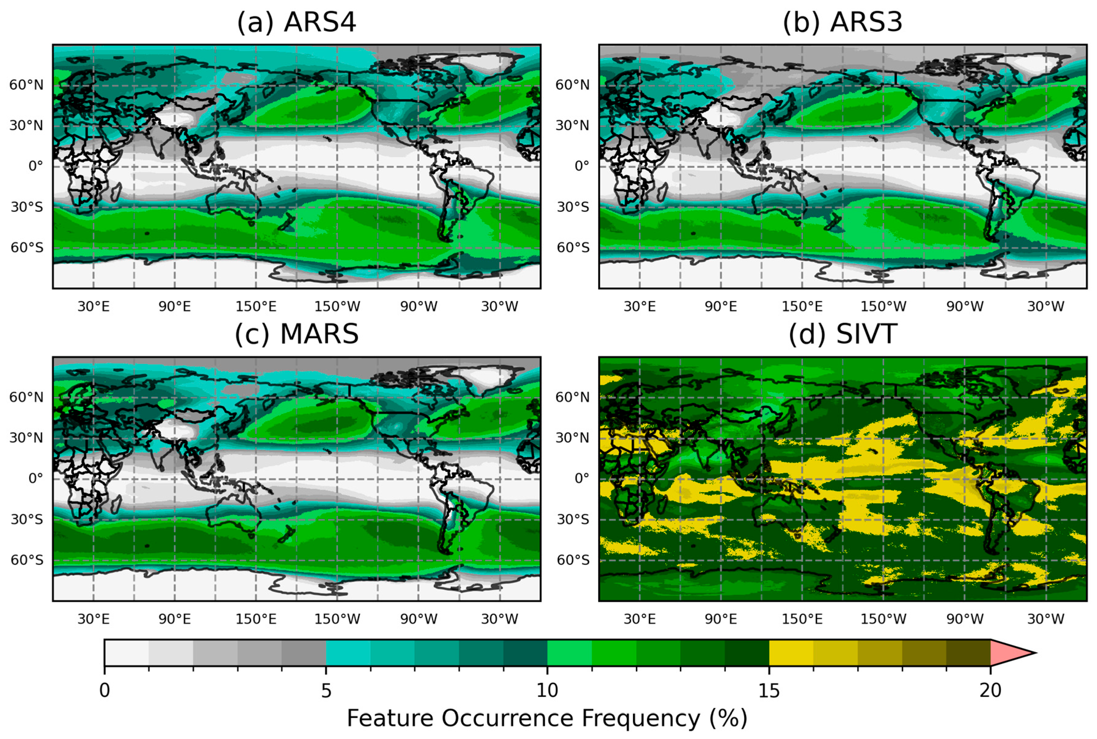
Figure 8 shows four FOF distributions based on the EDARA and S-EDARA data over a 30-year (1991-2020) period. For the global AR FOF patterns, strong agreements can be seen between the two tARget algorithm versions, with both capturing the well-established AR climatological features including storm track regions in the North Pacific and North Atlantic, AR activity along the coasts of western North America and western Europe, and Southern Hemisphere AR corridors. The tARget-v4 refinements resulted in negligible changes in the tropical climatological AR frequency and noticeable increases of AR activity over the polar regions (Figure 8a vs Figure 8b). The mid-latitude refinement led to slight increase (decrease) in AR FOF along the storm tracks in the Northern (Southern) Hemisphere.
The higher extratropical AR FOF values in Figure 8c as compared to those in Figure 8b are consistent with the removal of the poleward IVT requirement in mtARget-v3 algorithm north of 20°N and south of 20°S. Note that the tARget-v4 refinement also led to stronger polar AR activities in Figure 8a as compared to those in Figure 8c. This polar refinement in tARget-v4 is therefore related to the hemispheric IVT threshold applied on top of the pixel-wise IVT threshold that effectively increases the pixel-wise threshold to higher percentiles in cold/dry regions [19].
The much higher FOF values in Figure 8d serve as a reminder that the tARget algorithms use the IVT 85th percentile threshold as a necessary but not sufficient condition for AR detection. The specific coherence and geometry requirements further remove some high IVT features, especially those with entirely zonally-directed or equatorward IVT areas found in the tropics.
5. Usage Notes
5.1. Integration with EDARA
S-EDARA is designed as a supplement to the original EDARA dataset and is most powerful when used in combination with EDARA’s comprehensive meteorological variables. Users can merge the datasets using the common temporal and spatial grids, enabling analysis that combines tARget-v4 AR detection with the full suite of atmospheric variables provided in EDARA.
For studies requiring comparison between tARget v3 and v4 algorithms, both datasets should be used in parallel. This is particularly valuable for algorithm sensitivity studies and for assessing how AR detection methodology influences research conclusions about AR characteristics, trends, and impacts.
5.2. Threshold Sensitivity
The SIVT field is based on the 85th percentile threshold for local IVT climatology. Users should be aware that this threshold choice represents a balance between identifying meteorologically significant events and maintaining sufficient sample sizes for statistical analysis. For specific applications, users may wish to recalculate SIVT using different percentile thresholds (e.g., 90th or 95th percentile for more extreme events) based on the IVT data and the 4-level IVT percentiles provided in EDARA. Similarly, the 250 IVT threshold used in AR detection is a standard value in the AR research community, but some applications may benefit from sensitivity testing with alternative thresholds.
5.3. Regional Considerations
AR characteristics and impacts vary substantially across geographic regions. Users conducting regional studies should consider:
- Regional differences in AR frequency and seasonality
- Variations in the relationship between AR features and surface impacts
- Topographic influences on AR-related precipitation and wind patterns
The global coverage of S-EDARA enables comparative studies across regions, but care should be taken when generalizing results from one region to another.
5.4. Temporal Resolution
The 6-hourly temporal resolution of S-EDARA captures the primary evolution of AR features but may not resolve very rapid changes in AR intensity or structure. For applications requiring higher temporal resolution, users should consult the original ERA5 hourly data and consider processing additional time steps using the documented methodology.
5.5. Precipitation Proxy Limitations
PTPR provides a useful dynamical proxy for precipitation but should not be interpreted as a direct precipitation measurement. The relationship between moisture convergence and actual precipitation depends on numerous factors including atmospheric stability, lifting mechanisms, and microphysical processes that are not captured in PTPR. For quantitative precipitation analysis, PTPR should be used in conjunction with direct precipitation observations or ERA5 TPR data available in EDARA. It can also be used to define and refine some other proxies for precipitation, such as the primary condensation rate [22].
5.6. Computational Considerations
The full S-EDARA dataset represents a substantial data volume. Users working with limited computational resources may wish to:
- Download only specific months or years of interest
- Utilize the graphical catalogues for initial exploration before processing numerical data
- Consider cloud-based processing platforms for large-scale analysis
5.7. Citation and Attribution
Users of S-EDARA should cite both this data descriptor and the original EDARA dataset to ensure proper attribution to all contributors. When using the tARget AR detections, users should cite the relevant algorithm development papers [19,25,26,27]. Proper citation supports continued development and maintenance of community datasets and enables tracking of dataset usage and impact.
Funding
This research received no external funding.
Informed Consent Statement
Not applicable.
Data Availability Statement
The data presented in this study are openly available in the Federated Research Data Repository at: https://doi.org/10.20383/103.01528. Related Dataset: https://doi.org/10.20383/103.01542 [2,3]. Dataset License: CC-BY-4.0.
Conflicts of Interest
The authors declare no conflicts of interest.
References
- Mo, R. A Supplement to the ERA5-based Dataset for Atmospheric River Analysis (S-EDARA). Federated Research Data Repository 2025. [CrossRef]
- Mo, R. An ERA5-based Dataset for Atmospheric River Analysis (EDARA): Multi-decade numerical and graphical catalogues. Federated Research Data Repository 2024. [CrossRef]
- Mo, R. EDARA: An ERA5-based Dataset for Atmospheric River Analysis. Sci. Data 2024, 11, 900. [CrossRef]
- Newell, R.E.; Newell, N.E.; Zhu, Y.; Scott, C. Tropospheric rivers?–A pilot study. Geophys. Res. Lett. 1992, 19, 2401–2404. [CrossRef]
- Zhu, Y.; Newell, R.E. Atmospheric rivers and bombs. Geophys. Res. Lett. 1994, 21, 1999–2002. [CrossRef]
- Zhu, Y.; Newell, R.E. A proposed algorithm for moisture fluxes from atmospheric rivers. Mon. Wea. Rev. 1998, 126, 725–735. [CrossRef]
- Ralph, F.M.; Neiman, P.J.; Wick, G.A. Satellite and CALJET aircraft observations of atmospheric rivers over the eastern North Pacific Ocean during the winter of 1997/98. Mon. Wea. Rev. 2004, 132, 1721–1745. [CrossRef]
- Dettinger, M.D.; Ralph, F.M.; Das, T.; Neiman, P.J.; Cayan, D.R. Atmospheric rivers, floods and the water resources of California. Water 2011, 3, 445–478. [CrossRef]
- Gimeno, L.; Nieto, R.; Vázquez, M.; Lavers, D.A. Atmospheric rivers: A mini-review. Front. Earth Sci. 2014, 2:2. [CrossRef]
- Ralph, F.M.; Dettinger, M.; Lavers, D.; Gorodetskaya, I.V.; Martin, A.; Viale, M.; White, A.B.; Oakley, N.; Rutz, J.; Spackman, J.R. Atmospheric rivers emerge as a global science and applications focus. Bull. Am. Meteorol. Soc. 2017, 98, 1969–1973. [CrossRef]
- Waliser, D.; Guan, B. Extreme winds and precipitation during landfall of atmospheric rivers. Nat. Geosci. 2017, 10, 179–183. [CrossRef]
- Bozkurt, D.; Rondanelli, R.; Marín, J.C.; Garreaud, R. Foehn event triggered by an atmospheric river underlies record-setting temperature along continental Antarctica. J. Geophys. Res. Atmos. 2018, 123, 3871–3892. [CrossRef]
- Gonzales, K.R.; Swain, D.L.; Barnes, E.A.; Diffenbaugh, N.S. Moisture- versus wind-dominated flavors of atmospheric rivers. Geophys. Res. Lett. 2020, 47, e2020GL090042. [CrossRef]
- Bartells, J.H. Floods of November 19–25 in southwestern Washington. In Summary of Floods in the United States During 1962: Geological Survey Water-Supply Paper 1820, Rostvedt, J.O., Others, Eds.; U.S. Geological Survey: 1968; pp. 126–129.
- Samora, B.A. Chronology of Flood Events as noted in the Superintendent’s Annual Reports 1940-1991; Natural Resource Planning Division, Mount Rainier National Park, WA, USA: https://www.morageology.com/pubs/32.pdf, 1991.
- Septer, D. Flooding and Landslide Events Southern British Columbia 1808-2006 (Part 2: 1950-1979); Ministry of Environment, BC, Canada: https://www.env.gov.bc.ca/wsd/public_safety/flood/pdfs_word/floods_landslides_south2.pdf, 2007.
- Kulshreshtha, S.; Wittrock, V.; Magzul, L.; Wheaton, E. Impacts and adaptations to extreme climatic events in an aboriginal community: A case study of the Kainai Blood Indian Reserve. In The New Normal: The Canadian Prairies in a Changing Climate, Sauchyn, D., Diaz, H., Kulshreshtha, S., Eds.; CPRC Press, University of Regina: Regina, Saskatchewan, Canada, 2010; pp. 264–274.
- Hersbach, H.; Bell, B.; Berrisford, P.; Hirahara, S.; Horányi, A.; Muñoz-Sabater, J.; Nicolas, J.; Peubey, C.; Radu, R.; Schepers, D.; et al. The ERA5 global reanalysis. Q. J. R. Meteorol. Soc. 2020, 146, 1999–2049. [CrossRef]
- Guan, B.; Waliser, D.E. A regionally refined quarter-degree global atmospheric rivers database based on ERA5. Sci. Data 2024, 11, 440. [CrossRef]
- Lavers, D.A.; Villarini, G.; Allan, R.P.; Wood, E.F.; Wade, A.J. The detection of atmospheric rivers in atmospheric reanalyses and their links to British winter floods and the large-scale climatic circulation. J. Geophys. Res. Atmos. 2012, 117, D20106. [CrossRef]
- Rutz, J.J.; Steenburgh, W.J.; Ralph, F.M. Climatological characteristics of atmospheric rivers and their inland penetration over the western United States. Mon. Wea. Rev. 2014, 142, 905–921. [CrossRef]
- Mo, R.; So, R.; Brugman, M.M.; Mooney, C.; Liu, A.Q.; Jakob, M.; Castellan, A.; Vingarzan, R. Column relative humidity and primary condensation rate as two useful supplements to atmospheric river analysis. Water Resour. Res. 2021, 57, e2021WR029678. [CrossRef]
- Peixoto, J.P. Atmospheric Vapour Flux Computations for Hydrological Purposes; World Meteorological Organization: Geneva, Switzerland, 1973.
- Benton, G.S.; Estoque, M.A. Water-vapor transfer over the North American continent. J. Meteorol. 1954, 11, 462–477. [CrossRef]
- Guan, B.; Waliser, D.E. Detection of atmospheric rivers: Evaluation and application of an algorithm for global studies. J. Geophys. Res. Atmos. 2015, 120, 12514–12535. [CrossRef]
- Guan, B.; Waliser, D.E.; Ralph, F.M. An intercomparison between reanalysis and dropsonde observations of the total water vapor transport in individual atmospheric rivers. J. Hydrometeor. 2018, 19, 321–337. [CrossRef]
- Guan, B.; Waliser, D.E. Tracking atmospheric rivers globally: Spatial distributions and temporal evolution of life cycle characteristics. J. Geophys. Res. Atmos. 2019, 124, 12523–12552. [CrossRef]
- Agarwala, T. Heavy rainfall in several parts of India triggers floods, at least 11 dead. Reuters 1 July 2024, https://www.reuters.com/world/india/heavy-rainfall-several-parts-india-triggers-floods-least-11-dead-2024-07-02/.
- Wei, B. Thousands in need of rescue as severe floods hit Myanmar’s Myitkyina. The Irrawaddy 1 July 2024, https://www.irrawaddy.com/news/burma/thousands-in-need-of-rescue-as-severe-floods-hit-myanmars-myitkyina.html.
- Zou, S. Pingjiang in Hunan hit hard by major flooding. China Daily (Hong Kong Edition) 3 July 2024, p. 6.
- Zou, S. Town besieged by floodwaters is calling for reinforcements. China Daily (Hong Kong Edition) 4 July 2024, p. 8.
- Guo, Q.; Jiao, S.; Yang, Y.; Yu, Y.; Pan, Y. Assessment of urban flood disaster responses and causal analysis at different temporal scales based on social media data and machine learning algorithms. Int. J. Disaster Risk Reduct. 2025, 117, 105170. [CrossRef]
- Harris, R. Reservoir breach likely cause of silty torrent. Otago Daily Times 2 July 2024, p. 7.
- Vogt, C.; Heger, B. Seven dead after storms lash France, Switzerland and Italy. Digital Journal 2024, https://www.digitaljournal.com/world/seven-dead-after-storms-lash-france-switzerland-and-italy/article.
- Turner, J.; Lu, H.; King, J.C.; Carpentier, S.; Lazzara, M.; Phillips, T.; Wille, J. An extreme high temperature event in coastal East Antarctica associated with an atmospheric river and record summer downslope winds. Geophys. Res. Lett. 2022, 49, e2021GL097108. [CrossRef]
- Zou, X.; Rowe, P.M.; Gorodetskaya, I.; Bromwich, D.H.; Lazzara, M.A.; Cordero, R.R.; Zhang, Z.; Kawzenuk, B.; Cordeira, J.M.; Wille, J.D.; et al. Strong warming over the Antarctic Peninsula during combined atmospheric river and foehn events: Contribution of shortwave radiation and turbulence. J. Geophys. Res. Atmos. 2023, 128, e2022JD038138. [CrossRef]
- Kolbe, M.; Torres Alavez, J.A.; Mottram, R.; Bintanja, R.; van der Linden, E.C.; Stendel, M. Model performance and surface impacts of atmospheric river events in Antarctica. Discover Atmosphere 2025, 3, 4. [CrossRef]
- Wille, J.D.; Favier, V.; Gorodetskaya, I.V.; Agosta, C.; Baiman, R.; Barrett, J.E.; Barthelemy, L.; Boza, B.; Bozkurt, D.; Casado, M.; et al. Atmospheric rivers in Antarctica. Nat. Rev. Earth Environ. 2025, 6, 178–192. [CrossRef]
Figure 1.
A snapshot of an Atmospheric River (AR) and the associated hydrometeorological impacts valid at 0000 UTC 20 November 1962; The plot is based on the ERA5 reanalysis dataset and the AR boundary (marked by a blue line) is determined by the tARget-v4 algorithm. (a) The Integrated Vapour Transport (IVT) is plotted in coloured contours and its vector representation (IVF: Integrated Vapour Flux) is indicated by white vectors. (b) The Total Precipitation Rate (TPR) is the sum of the rates of convective and large-scale rain and snowfall water equivalent. (c) The gusty wind speed is defined as the larger value between instantaneous wind speed and wind gust measured at 10 metres above ground. (d) The temperature difference between the current hour and 24 hours earlier at 2 metres above ground.
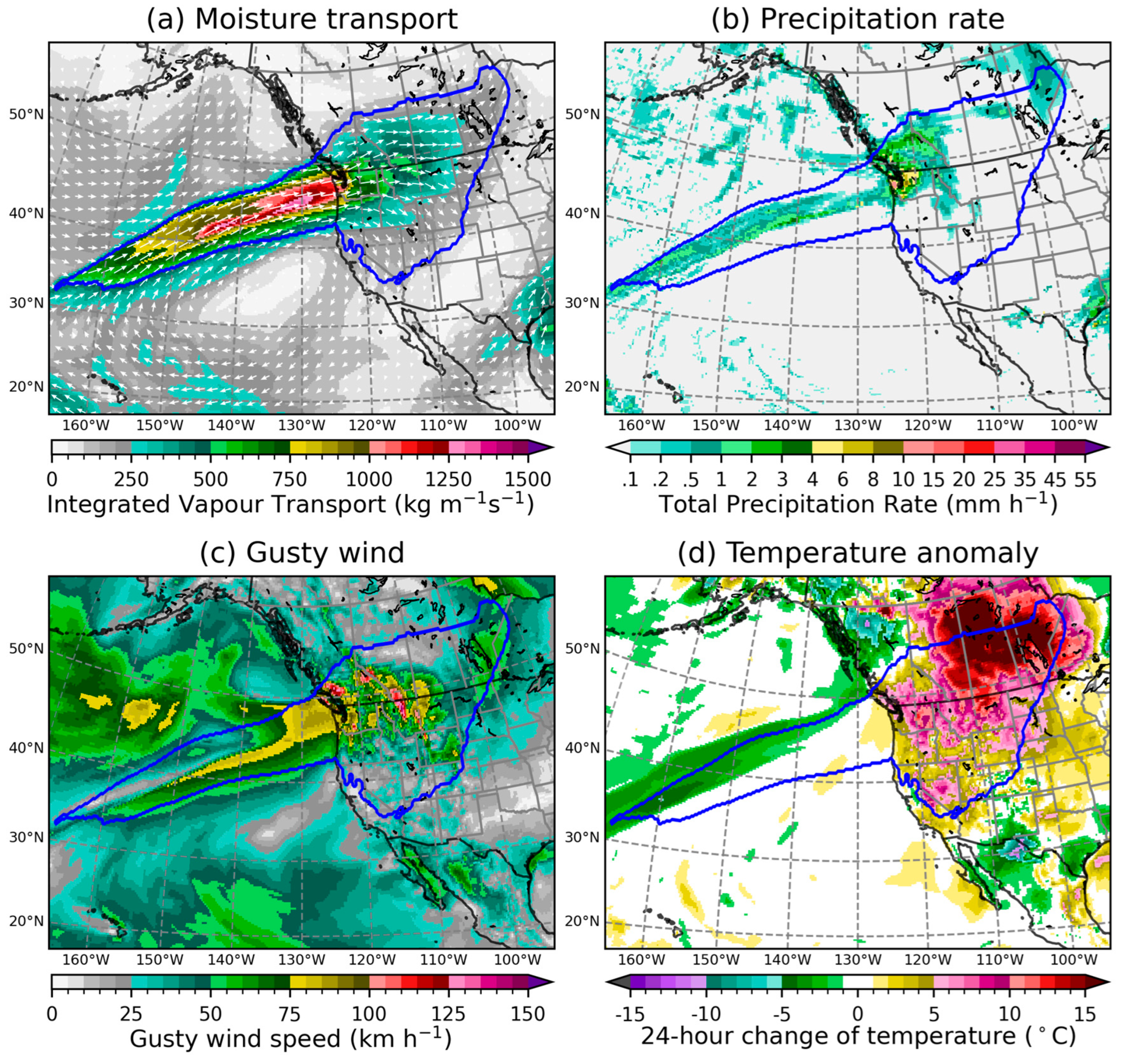
Figure 2.
The PTPR distribution valid at 0000 UTC 20 November 1962, which is comparable to the TPR distribution plotted in Figure 1b. The AR boundary (blue line) is determined by the tARget-v4 algorithm.
Figure 2.
The PTPR distribution valid at 0000 UTC 20 November 1962, which is comparable to the TPR distribution plotted in Figure 1b. The AR boundary (blue line) is determined by the tARget-v4 algorithm.
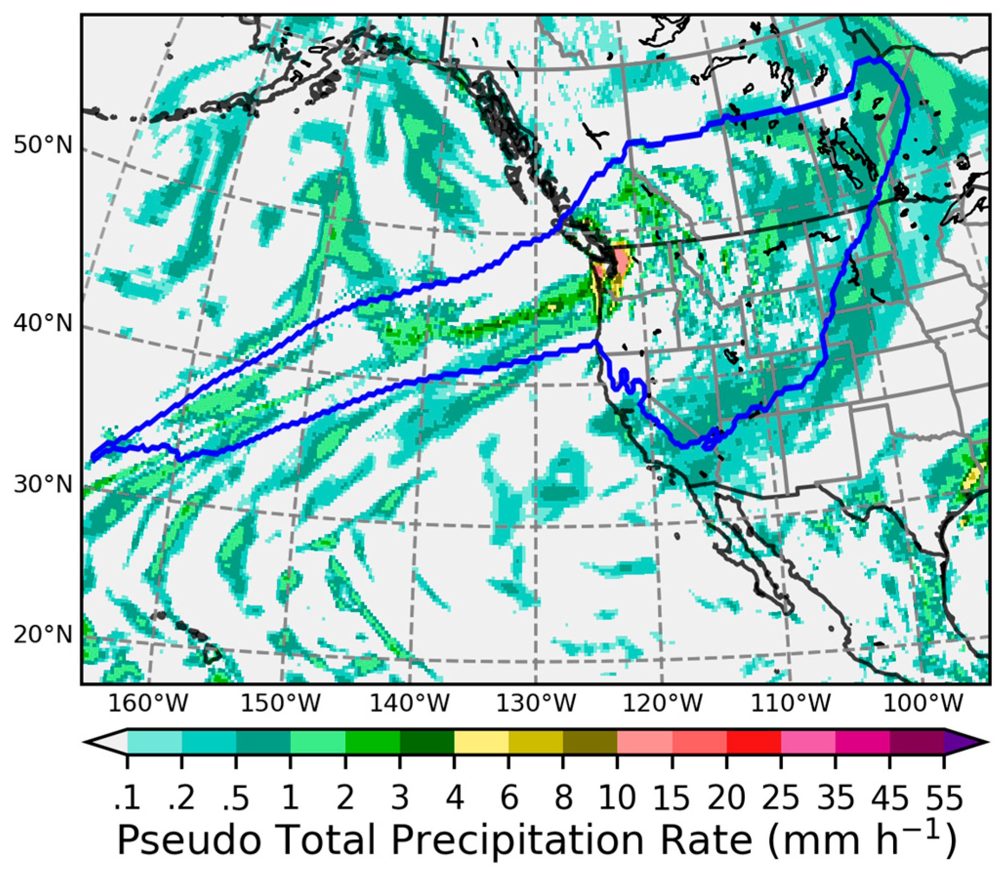
Figure 3.
The interface of graphical atmospheric river catalogue for June 2024. The AR boundaries determined by the tARget-v4 algorithm (ARS4 = 1) are marked by blue lines in (a), (c), and (d). The blue lines in (b) mark the boundaries of SIVT = 1. The IVT and IVF distributions are shown in (a). The distributions of PTPR, GWS10m, and CT24h are shown in (b), (c), and (d), respectively. Convenient settings are available for running animation through the whole month at a 6-hour time step and for switching between different months. Further information can be found by clicking the “About…” button.
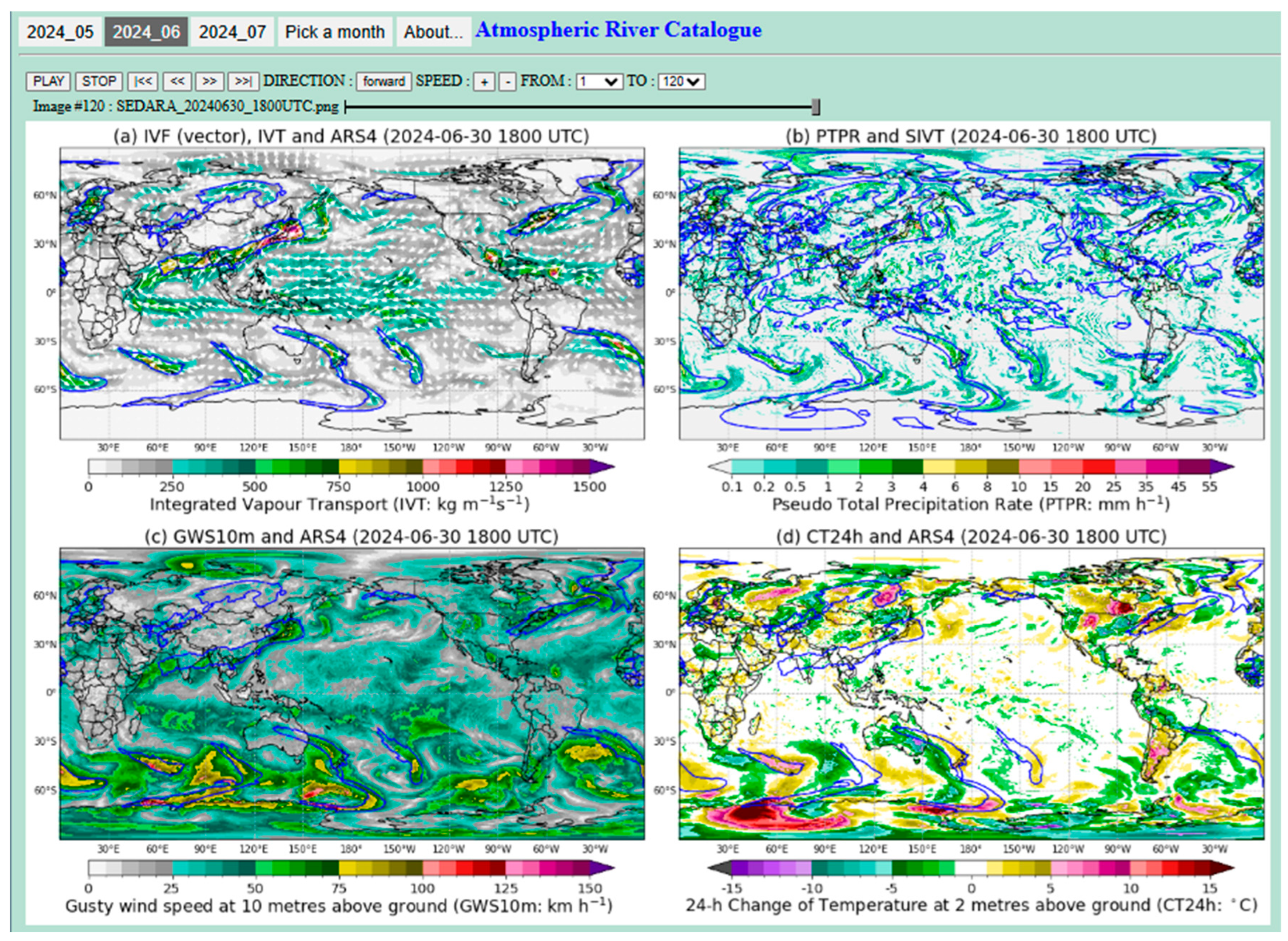
Figure 4.
The atmospheric river features at 1800 UTC 30 June 2024, detected by the tARget-v3 and mtARget-v3 algorithms, available from the EDARA graphical AR catalogue (Global Domain) [2,3]. The AR boundaries determined by the tARget-v3 algorithm and a modified version of it (mtARget-v3) are marked on the maps by red dashed lines and blue solid lines, respectively. The top panel also shows the IVT distribution and its vector representation (Qu, Qv). The total precipitation rate (TPR) distribution is shown in the bottom panel.
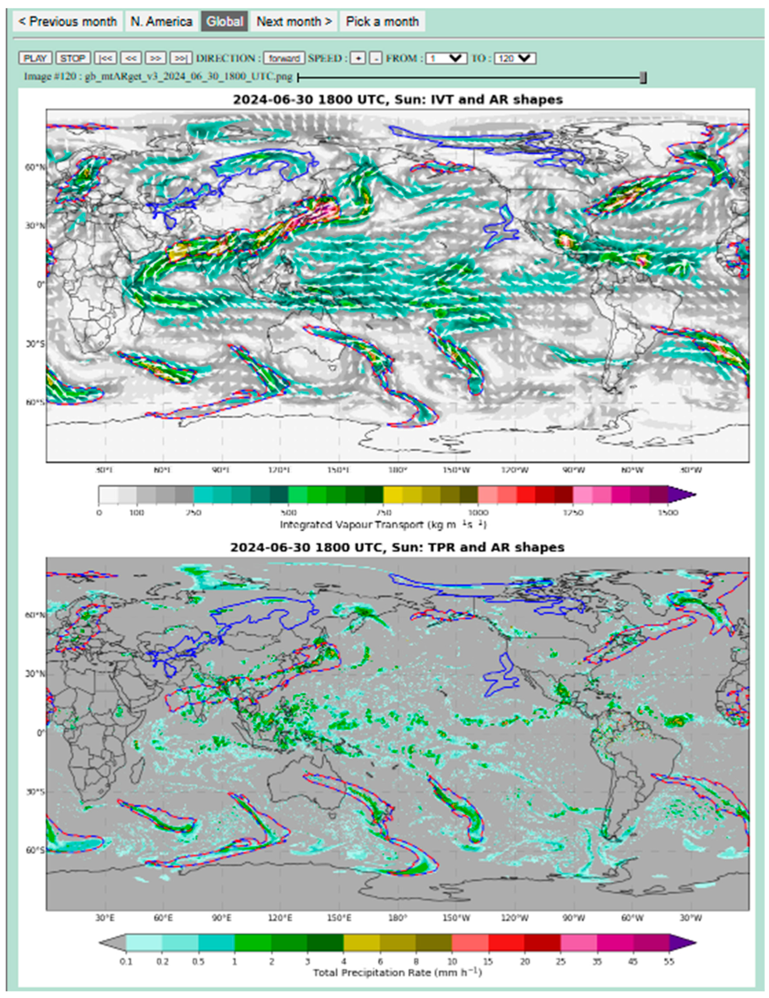
Figure 5.
A composite radar map over Europe valid at 1800 UTC 30 June 2024, obtained from https://en.tutiempo.net/europe/radar. .
Figure 5.
A composite radar map over Europe valid at 1800 UTC 30 June 2024, obtained from https://en.tutiempo.net/europe/radar. .
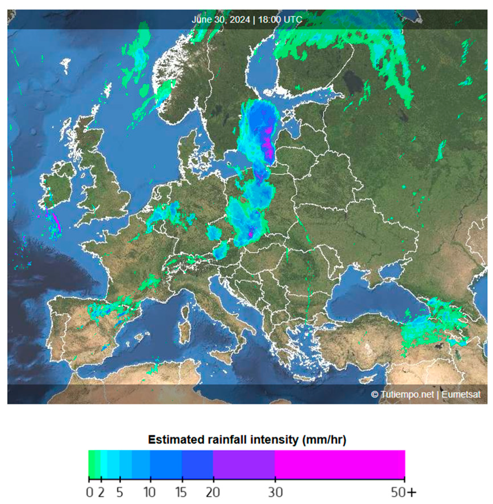
Figure 6.
The distributions of (a) TPR and (b) PTPR in Europe valid at 1800 UTC 30 June 2024. The tARget-v4 AR boundaries are marked by blue lines in the maps.
Figure 6.
The distributions of (a) TPR and (b) PTPR in Europe valid at 1800 UTC 30 June 2024. The tARget-v4 AR boundaries are marked by blue lines in the maps.
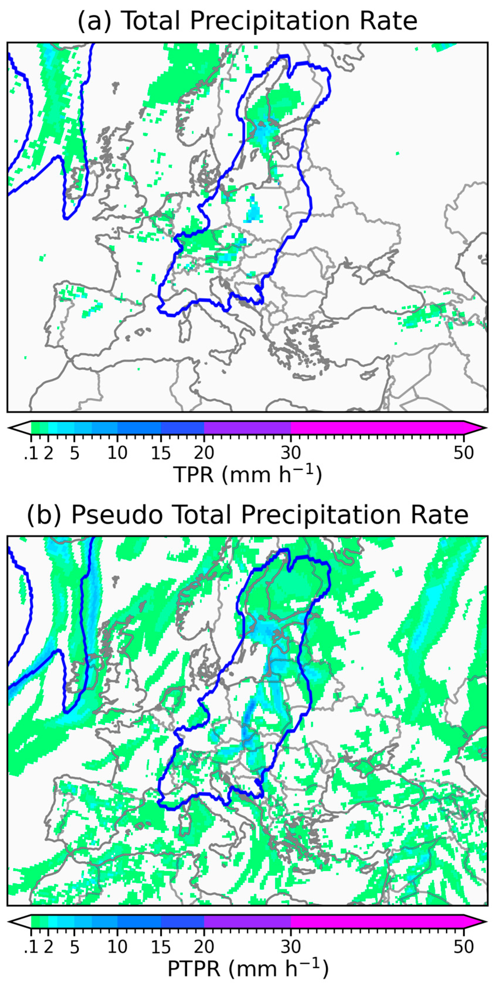
Figure 7.
A zoom-in view of Figure 3 focusing on the Atlantic tropical storms valid at 1800 UTC 30 June 2024.
Figure 7.
A zoom-in view of Figure 3 focusing on the Atlantic tropical storms valid at 1800 UTC 30 June 2024.
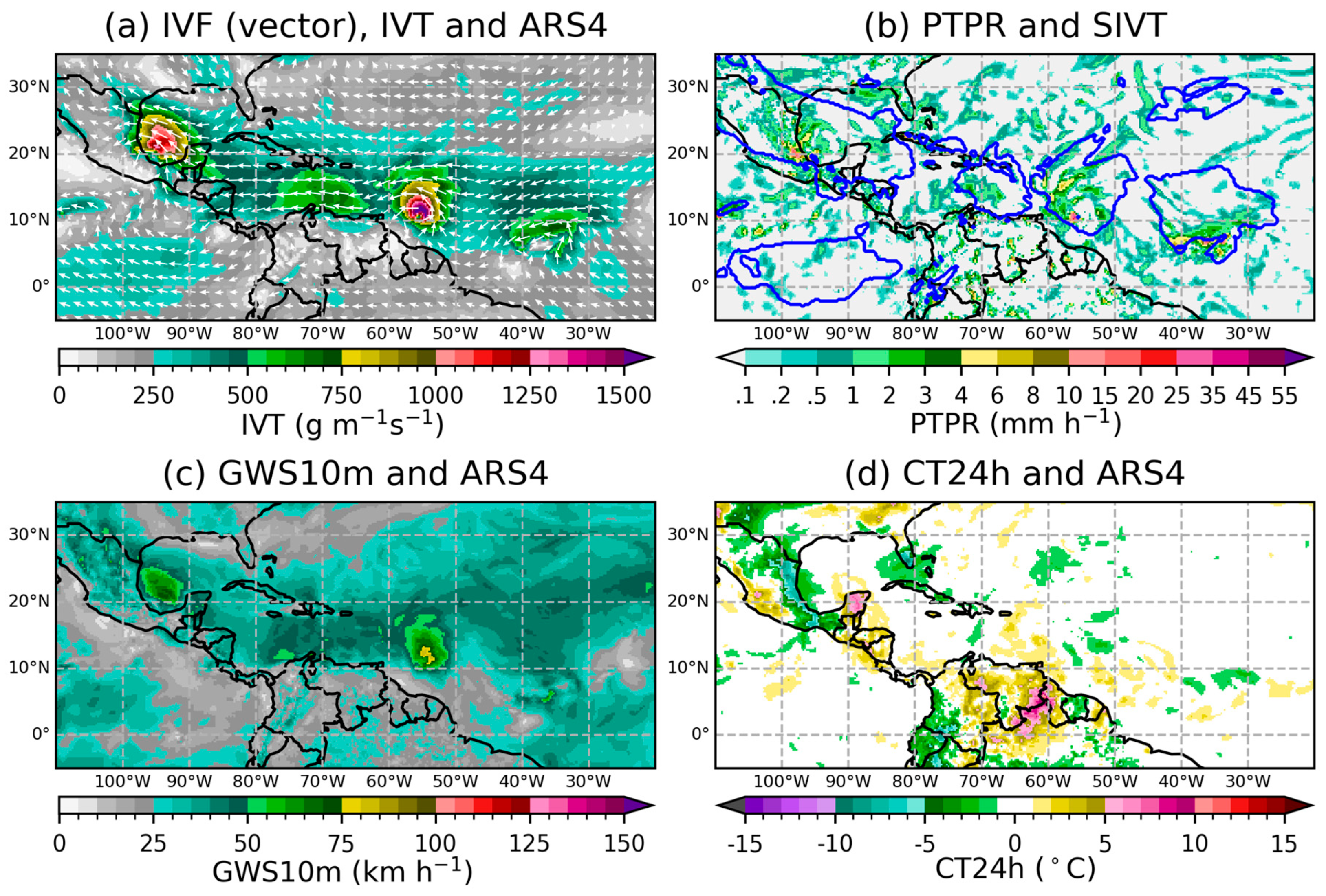
Figure 8.
Global distributions of the feature occurrence frequency (FOF) of (a) ARS4 from S-EDARA (based on tARget-v4), (b) ARS from EDARA (based on tARget-v3), (c) MARS from EDARA (based on mtARget-v3), and (d) SIVT from S-EDARA. The FOFs are computed from EDARA data over a 30-year (1991-2020) period. .
Disclaimer/Publisher’s Note: The statements, opinions and data contained in all publications are solely those of the individual author(s) and contributor(s) and not of MDPI and/or the editor(s). MDPI and/or the editor(s) disclaim responsibility for any injury to people or property resulting from any ideas, methods, instructions or products referred to in the content. |
© 2026 by the authors. Licensee MDPI, Basel, Switzerland. This article is an open access article distributed under the terms and conditions of the Creative Commons Attribution (CC BY) license (http://creativecommons.org/licenses/by/4.0/).
Copyright: This open access article is published under a Creative Commons CC BY 4.0 license, which permit the free download, distribution, and reuse, provided that the author and preprint are cited in any reuse.


