
Submitted:
15 October 2025
Posted:
16 October 2025
You are already at the latest version
Abstract
IDF curves are widely used to develop the design storm and usually remain in use for long periods of time. However, continuous data collection and the addition of new monitoring stations require updates to the existing curves. In Romania, current prac-tice is still based on curves established in 1973. Climate change significantly alters the frequency and mostly the intensity of extreme rainfall events, justifying the need to update the IDF curves. In addition to using recent observations, updating these curves is essential to support the adaptation of infrastructure to changing climatic conditions. This study analyzed the IDF curves from 68 meteorological stations using data records from the last 30 years.
Different approaches were analyzed to obtain a new regionalization, including clus-tering, geographic proximity, or hourly precipitation isolines for a frequency of 1:10. Using rasterized regional rainfall data obtained based on the 1973 and 2025 IDF curves, percentage precipitation differences were calculated. The results indicate that the value of short-term precipitation (5’, 10’, 30’) increased in most of Romania, while long-term events (3 h, 6 h, 12 h or 24 h) largely recorded a decrease in precipitation value in many areas. The increase in short-term torrential rainfall highlights the need for active prevention and management of urban flash floods.
Keywords:
IDF curves
; regionalization
; raster data
; rainfall torrentiality
; adaptation measures
1. Introduction
IDF (Intensity–Duration–Frequency) curves numerically express the average intensity of the maximum annual rainfall as a function of the duration of the rainfall and its frequency or return period [1,2]. Koutsoyiannis et al [3] emphasized that the term “frequency” should be understood as the annual frequency of exceedance (AFE). The IDF relationship can be expressed mathematically as:
where is the duration of rainfall, and is the average number of years for which a rainfall of duration is equaled or exceeded; is the AFE i.e. the frequency at which a certain intensity is equaled or exceeded in years.
The IDF curves represent empirical relationships resulting from the statistical processing of precipitation for different rainfall durations. For each duration the maximum intensities recorded for 30 years represent the statistical series.
In the analysis of extreme events, whether it is maximum flows, rainfall, temperatures etc., either annual maximum values (AMS = annual maxima series, also called Block Maxima = BM) or values above a given threshold (PDS = partial duration series or annual exceedance series method, also called Peak Over Threshold = POT) are processed [1,3,4,5,6,7]. The AMS or BM was the first approach used since the beginning of extreme events analysis in hydrology [8,9], while the PDS or POT approach was developed over the last 50 years by different researchers and synthetized mainly by Cunnane [10,11,12,13].
In the case of the POT approach, consecutive values must be independent, and the threshold must be chosen such that the series of selected events counts values [3,14]. If the threshold is not or cannot be set appropriately and the number of selected values is greater or less than the number of years , the corresponding probabilities must be converted into annual exceedance probabilities [15]. If a low threshold is selected, serial correlation may be observed.
Numerous works deal with the comparison of BM and POT, applied to maximum flow [16,17,18,19,20] or to rainfall intensity [7,14,21,22].
The following distributions are commonly used for rainfall processing: the Extreme Value Type I or Gumbel distribution [1,6], the Pearson type III distribution [23], the generalized Pareto distribution (GP) [7]. Other distributions, although not frequently used in current practice [3]are: the Generalised extreme value (GEV) distribution which, in addition to the Gumbel distribution (EV I), also includes type II and III extreme value distributions of maxima, the 2-parameter Gama distribution, the Log Pearson III distribution, the lognormal distribution, the exponential distribution, and the three parameter Pareto distribution.
The most used model is the Gumbel distribution due to its ease of use, involving only two parameters (mean and standard deviation), while in the case of 3 parameters models the skewness (whose estimation is affected by high uncertainties) must be calculated [24]. Ben-Zvi [7] showed that, for his case studies, the Gumbel and lognormal distributions fit most AMS and very few PDS, while in almost all cases the GP distribution fits PDS well. Another of his results is that the GP distribution does not fit AMS. RainIDF is a software tool for automatically deriving of IDF relationship from annual maxima and partial duration series, using the Generalized Extreme Value (GEV) distribution for annual maxima series, and the Generalized Pareto (GPA) distribution for Partial Duration Series [25].
Traditionally, in many countries, as well as in Romania, the analysis of maximum rainfall is based on the Gumbel distribution applied to the AMS, without even considering the PDS. However, Koutsoyiannis [14,22,24] showed that the Gumbel distribution underestimates extreme rainfall values for large series, while for a typical duration of several decades of records it can be an adequate model, suggesting that the better alternative for the analysis of extreme rainfall is the use of the EV type II distribution (Fréchet distribution).
The relationships determined at meteorological stations can also be used for adjacent areas, considered meteorologically homogeneous, up to 50 km2. The rainfall duration defining the IDF curves is between 5 minutes and 1440 minutes, with a temporal resolution of 5 minutes up to a rainfall duration of 120 minutes and then with a rarer cadence (140’; 160’; 180’; 240’; 300’; 360’; 720’; 1440’). IDF curves values are typically provided for the following frequencies: .
IDF curves are used for:
- Determining design storm to establish design or verification flows for the rehabilitation and extension of the existing sewerage system, or for new sewerage networks.
- Establishing the necessary measures for flood risk management, mainly in urban drainage basins, but also in small catchments.
- Providing meteorological information for making decisions in spatial planning involving changes in current land use.
If data at a higher temporal resolution are missing or sparce, daily rainfall data, which are usually available, can be used to derive IDF curves for short-duration events based on scale properties [3,26].
Talbot proposed the first empirical IDF relationship in 1881 (Sosrodarsono and Takeda, 1983, cited by [27]), followed by many other authors such as Sherman (1905), Bernard (1932), Wenzel (1982), Kimijima, Koutsoyannis (1998) [1,3,23].
The intensity of rainfall is inversely proportional to the storm duration raised to a power, which represents a scaling factor [3]. The most general expression of the IDF curves was provided by Koutsoyiannis et al [3]:
where is the average rainfall intensity for the duration of the rainfall, while the other coefficients that are non-negative. The nominator depends on frequency of rainfall, while the denominator is a function of rainfall duration [3]. The denominator determines the shape of the curves as follows: is the slope of the linear part of the IDF curves, while determines the curvature change point [28]. All relations currently used for IDF curves are obtained as specific cases of relation (1), adopting or as appropriate [3]. Koutsoyiannis and al [3] showed that the coefficients must satisfy the following sets of constraints to avoid intersection of IDF curves:
For in relation (1), the Sherman equation is obtained:
where is the average rainfall intensity over the rainfall duration, while , and are non-negative coefficients.
The following equivalence can be established between the coefficients of relations (2) and (3):
IDF curves are calculated for each weather station. The least squares method is then used to obtain the on-site parameters. At-site Frequency Analysis (AFA) can give misleading results, especially in the case of short period of available data. The solution is to divide the area of interest into homogeneous regions [29,30]. This procedure of regional frequency analysis is called “regionalization”.
Regional Frequency Analysis (RFA) overcomes the limitations of AFA (short duration availability of historical rainfall data, which leads to significant uncertainty for their extremes estimation) by aggregating data from all stations located into a homogeneous region (enhancing thus the sample size and implicitly the robustness of quantile estimates) [30]. To ensure statistical accuracy in the case of RFA, all rainfall datasets should cover, if possible, the same recording period. RFA has proven its superiority over AFA for low frequencies (1:30; 1:50; 1:100), while AFA has demonstrated better performance for high frequencies (1:2; 1:3) if the volume of the sample is adequate [30].
Regionalization based on homogeneous regions also has limitations, as highlighted by Deidda et al. [31], including: discontinuities in estimating quantiles along boundaries, neglecting the influence of local orography and climatology, under- or over-estimating quantiles even at the site level, due to the average distribution assigned to each homogeneous region. The alternative to the regional approach based on homogeneous regions is a boundaryless approach, based on geostatistical interpolation of at-site estimates of all distribution parameters [31,32]. The boundaryless approach is, in fact, a generalization of classical regionalization.
Different procedures can be used to achieve regionalization. Based on local IDF relationships, maps of regional rainfall intensities or rainfall depths for different durations and frequencies have been provided in the past [1,8]. Other authors have derived isolines of the IDF parameters for each AFE. In this way, Nhat et al. [23] obtained contour maps in Vietnam for the three parameters of the Kimijima formula. Using these maps, IDF curves can be obtained for any location, corresponding to different AFE. Another approach, used for a long time, consists in dividing the country or region of interest into homogeneous zones, providing a set of IDF curves for each zone.
The objective of this paper is to analyze different approaches to obtain the regionalization of IDF for the entire territory of Romania: a) clustering methods (k-means, DBSCAN and Hierarchical Clustering) b) isolines of the statistical parameters of the maximum daily annual rainfall; c) similarities between the IDF curves of the meteorological stations and d) isolines of the 1-hour rainfall depth for the frequency 1:10. By comparing the different methods and analyzing the weaknesses of each of them, it was finally decided to adopt the isolines of the 1-hour rainfall depth, frequency 1:10, for the regionalization of the IDF relations. Ten quasi-homogeneous zones resulted, for each zone the station with the most unfavorable values of the IDF curves being selected as representative.
The paper is organized as follows: the first section is the Introduction, Section 2 provides a description of the study area, the methodological framework of the research, the approach to investigating climate change and the least squares method for calculating the parameters of the Sherman equation. Section 3 illustrates the results obtained with each of these approaches, highlighting their limitations where appropriate. Section 4 contains comments related to the coefficients , and , which are specific to each region and depend on the AFE. The corresponding constraints are highlighted. Section 5 presents the main conclusions and future research directions.
2. Materials and Methods
2.1. Study Area
Romania has an area of 238,397 km2, located in southeastern Europe and bordered by Ukraine, Hungary, Serbia, Bulgaria, Moldova and the Black Sea. It lies between latitudes 43° and 49° N and longitudes 20° and 30° E. The Carpathian Mountains dominate central Romania, surrounded by the plateaus of Moldavia and Transylvania, the Pannonian Plain and the plains of Wallachia [33]. Romania has a continental climate, with some regional differences: Mediterranean influences in the western regions (mainly in Banat), a more pronounced continental climate in the eastern part of the country, while the Black Sea exerts its influence in Dobrogea (Figure 1).
The main types of atmospheric circulation that lead to heavy rainfall, resulting in significant flooding [34] are:
• The western circulation, of oceanic origin, occurs when at the same time, in the southern part of Europe there is an anticyclonic field (high pressure), and in the northern areas there are depression nuclei. During the summer, this type of circulation favors the production of high intensity and short-term rains.
• The northern or north-western circulation brings moist air masses of oceanic origin to Central and South-Eastern Europe. This type of circulation, which manifests itself in the spring-summer and autumn periods, produces sudden drops in air temperature and favors the formation of torrential rainfall.
• The southern or southeastern circulation is characterized by a strong advection of warm air, loaded with a lot of moisture when passing over the Mediterranean Sea. In summer, it causes unstable weather, generating heavy rains, especially in the form of showers.
Significant amounts of rain falling in short periods of time are linked to the peculiarities of the evolution of cyclones, especially those of a Mediterranean nature. The evolution of cyclones is often closely linked to the orographic conditions existing in the areas of movement of these cyclones. High intensity rains, lasting between 8-12 hours and 24-72 hours, produce general flooding on basin areas ranging from 3,000 to 25,000 km2. These areas experience extremely intense rain cores, lasting 2-3 hours (or even less), which lead to the formation of local flash floods.
Sewerage systems in Romania have traditionally been designed for frequencies ranging from 2:1 (for villages or small towns) to 1:3 (for large cities). These values are common for many European countries, although for some more important components the design frequency can be extended to 1:50 [22]. The EU standard EN 752-2 [35] recommends (Table 1) rainfall design frequencies for gravity drainage systems outside buildings in the range of 1:1 to 1:10.
Urban flooding occurs less frequently than the Design Storm frequency because sewers are designed to operate without surcharge. Under “pressurized” flow conditions, they have a much higher flow capacity, meaning that street flooding occurs at a lower frequency [36,37].
The new Romanian regulations [38] established frequencies of 1:5 for localities under 100,000 inhabitants and 1:10 for cities with over 100,000 inhabitants. The regionalization currently used, developed in 1973 [39], is based on IDF curves from 19 significant meteorological stations, selected from the total number of stations existing in Romania at that time (Figure 2). This regionalization is mainly based on geographical and geomorphological criteria.
2.2. Research Framework
Meteorological data is collected continuously, and new monitoring stations have been commissioned in Romania since 1973, which requires updating of previous IDF curves to support the adaptation of infrastructure to changing climate conditions. Climate change plays a key role by significantly modifying the frequency and intensity of extreme rainfall events, justifying the need for updates. High values of the Hurst index indicate with a high probability an upward trend in the frequency of extreme rainfall [40].
To highlight climate change, rainfall data from the last 30 years were used for analysis, and the results were compared with the IDF curves obtained in 1973. Of the 102 stations with continuous records, only 68 were selected based on their relevance in terms of proximity to human settlements with over 2000 inhabitants. The IDF curves were provided by the National Meteorological Administration of Romania (ANM).
Proper regionalization is a prerequisite for regional frequency analysis (RFA) of rainfall. Different approaches have been tested to obtain the most reasonable regionalization, as follows:
- The first approach used the annual maximum daily rainfall. The stations were grouped according to their coefficient of variation, applying different clustering methods: k-means, DBSCAN, and Hierarchical Clustering.
- For the same annual maximum daily rainfall of the meteorological stations, contour maps were obtained for each parameter (mean value, standard deviation, coefficient of variation) which were then analyzed in relation to their plausibility.
- Another attempt at regionalization consisted in searching for similarities between any pair of two stations. Similarity was accepted for the correlation coefficient and the Nash-Sutcliffe efficiency coefficient higher than 0.99.
- Another approach was regionalization based on the 1-hour rainfall depth for each station corresponding to the frequency of 1:10.
To highlight climate change, the percentage differences between the rasters corresponding to the 2025 regionalization (based on the 1-hour maximum depth) and the 1973 regionalization were calculated. A flowchart of the procedures adopted is presented in Figure 3.
2.2.1. Clustering
As previously shown, homogeneous regions can be determined based on cluster analysis, which classifies available data into similar overlapping or non-overlapping groups (Goyal and Gupta, 2014). Validity indices, such as Partition Coefficient, Partition Entropy, Extended Xie-Beni index, Fukuyama-Sugeno index or Kwon index can be used to discriminate between partitions provided by different clustering algorithms [29].
•k-means
The k-means algorithm is based on the Euclidean distance between points, calculated as follows:
In this study, 68 stations were grouped using the coefficient of variation as the main attribute.
•DBSCAN (Density-Based Spatial Clustering of Applications with Noise)
Unlike k-means, which relies on centroid-based clustering and requires the number of clusters k to be specified in advance, DBSCAN groups points based on density, forming clusters in regions with a high concentration of points. Additionally, DBSCAN can detect outliers, a feature that k-means does not offer. The DBSCAN algorithm requires two key parameters: the maximum distance between two points to be considered neighbors, and the minimum number of points required to form a cluster. This dependence makes the algorithm very sensitive to parameter selection.
•Hierarchical Clustering
This algorithm constructs a dendrogram that represents the hierarchy of similarities between points (Figure 6), without the need to predefine the number of clusters. The dendrogram can then be cut at any level chosen to obtain the desired number of clusters.
2.2.2. Isolines of statistical parameters of the annual series of maximum daily rainfall
These maps show the isolines of the main statistical parameters (mean, standard deviation, and coefficient of variation) calculated for the annual series of maximum daily rainfall at each station.
Annual series of maximum daily rainfall have been used for their studies by many researchers. For instance, Koutsoyiannis, [24], Koutsoyiannis and Baloutsos [41] analyzed the annual series of maximum daily rainfall in Athens, Greece, extending through 1860-1995. Kuo et al [42] investigated the trends of annual maximum rainfall during heavy rainfall events in southern Taiwan, both for 24-h and 1-h duration. Deidda et al [31], Minguez and Herrera [32] also used 24-h rainfall in their studies of extreme events in Sardinia and the Basque Country, respectively. Given the interest that the analysis of annual raifall maxima at a daily resolution still presents, the isolines of the statistical parameters for 24-hour precipitation were obtained within the study.
2.2.3. Similarities between meteorological stations
The similarities between the IDF curves at any pair of two stations (e.g., station i, and station j) were evaluated based on the Coefficient of Determination and the Nash–Sutcliffe Efficiency (NSE) metric. By using these metrics, a more reliable and detailed assessment is provided compared to traditional metrics [43].
• The Coefficient of Determination
• The Nash–Sutcliffe Efficiency coefficient (NSE) is calculated as one minus the ratio of the error variance between time series i and j, divided by the variance of time series j.
where and are the rainfall intensities at stations i and j respectively for durations taking values in the range 5 minutes - 1440 minutes, while and are the mean values of the rainfall intensities at the two stations.
2.2.4. Isolines of the 1-hour accumulated rainfall depth corresponding to the frequency of 1:10
The isolines were drawn for a discretization step of 2 mm, resulting in ten homogeneous zones. To characterize an area located between two neighboring isolines, the IDF curve with the highest values is chosen for safety reasons.
2.2.5. Investigating climate change
Based on raster data for regionalized rainfall from 1973 and 2025, the percentage differences in precipitation between these years were calculated for the following durations: 5’, 10’, 30’, 60’, 3h; 6h; 12h and 24h. The resulting maps highlighted the change in rainfall regime between 1973 and 2025 for each of these durations.
2.2.6. Using the Sherman relation for IDF curves
If the concentration time corresponding to a locality is between the tabulated time values and it is necessary to interpolate the intensity value, the Sherman analytical expression can be used to approximate the IDF curve:
where:
a, b, and c are the parameters of the IDF curve corresponding to the chosen frequency,
= is the rainfall duration assumed to be equal to the concentration time .
The parameter values for each rainfall frequency and each area of the ten homogeneous zones were obtained by the method of least squares, minimizing the function:
where:
is the value of the rainfall intensity corresponding to the analyzed frequency for the standard durations from 5 minutes to 1440 minutes.
a, b, and c are specific parameters for each frequency and homogeneous zone.
3. Results
3.1. Clustering
The spatial distribution of meteorological stations across Romania, shown in Figure 4 and colored according to the coefficient of variation, indicates that the stations are uniformly distributed at national level. Clustering methods were applied to regionalize the stations, allowing the identification of climatic regions with similar behaviors based on the spatial analysis of meteorological phenomena [41,42,43,44,45,46,47,48,49]. Clustering in hydrology and meteorology is valuable for regionalizing precipitation and temperature models because it groups stations with similar climate profiles. It also reduces data complexity by aggregating information into meaningful groups, helps identify areas at high risk of extreme events, and provides a basis for climatic and hydrological modeling, facilitating regional interpolation and estimates. Therefore, the clustering approach serves not only to classify stations, but also to understand spatial structures and climate variability at national and regional scales [44,45,46,50,51].
- k-means
The optimal number of clusters was determined using the Elbow method (WSS) (Figure 5a) and the Gap Statistic method (Figure 5b).
Both methods resulted in an optimal number of seven clusters. The quality of clustering was assessed using the average Silhouette score (Figure 6). A score close to 1.0 indicates well-separated clusters, 0.5–0.7 means good clustering, 0.3–0.5 indicates moderate clustering, and below 0.3 indicates poor clustering. The average Silhouette score for the seven clusters was 0.342, which means moderate clustering quality. The clusters obtained with k-means can be seen in Figure 7.
- DBSCAN
DBSCAN produced an optimal clustering with four clusters. The average Silhou-ette score was low (0.17), indicating poor clustering quality. This suggests that DBSCAN is not suitable for uniformly distributed stations, as it is based on point density.
- Hierarchical Clustering
The similarity tree (dendrogram) of the points is shown in Figure 8. An optimal number of seven clusters also resulted (Figure 9), while the average Silhouette Index increased slightly to 0.345 (Figure 10).
Comparison of the k-means clustering (Figure 6) and hierarchical clustering (Figure 11) shows very similar results. For both methods, the Hosking homogeneity index was calculated for each cluster, indicating that the clusters are homogeneous. However, clustering does not ensure complete national coverage, as large areas remain outside the identified clusters.
3.2. Isolines of the Main Parameters for the Annual Maximum Daily Rainfall
Figure 12, Figure 13 and Figure 14 show maps with isolines for each parameter (mean, standard deviation, and coefficient of variation).
These maps illustrate the spatial variability of daily precipitation over Romania. Of these, only the isolines of the coefficient of variation provide a plausible basis for regionalization. However, for practical applications, sub-daily rainfall is of greater importance.
3.3. Similarities Between Meteorological Stations
The similarity between any pair of stations (e.g., station i and station j) were quantified based on the Coefficient of Determination and the Nash–Sutcliffe Efficiency (NSE) metric. The coefficients of similarity ( and NSE), can be represented as an upper triangular matrix due to the symmetry between the pairs of stations.
Table 2 presents the NSE coefficients for a few randomly selected stations. While in some cases, stations and are located close to each other and may belong to the same homogeneous polygon, in other cases they are located at very large distances. For example, the municipality of Arad has high NSE values with Lugoj and Timișoara located at 69.62 km and 49.48 km, respectively, but an even higher value with Fetești and Bîrlad located at 546.98 km and 488.40 km, respectively.
The high NSE values result from considering all rainfall durations from 5 to 1440 minutes. For shorter rainfall durations (e.g., 3 or 6 hours), the NSE values decrease, but the overall conclusion remains the same: both and NSE indicate pointwise similarities but cannot be used to delineate regional patterns.
3.4. Regionalization Based on 1-Hour Accumulated Rainfall Depth
Urban catchments are relatively small and typically have a response time of less than 1 hour (Fletcher et al [54]. Bell [52] developed a generalized IDF formula using 1-hour rainfall depth. In addition to the maximum annual rainfall depths for a 24-hour duration, Kuo et al (2011) also analyzed the maximum annual rainfall depths for a 1-hour duration. Numerous other studies use 1-hour rainfall as a standard. Thus, sub-daily rainfall, including 1-hour, 3-hour and 6-hour maxima, has been studied extensively in the Pannonian Basin [53]. The investigation of extreme sub-daily rainfall is justified by the potential for flash floods, especially in mountainous areas [53]. High intensity, short duration rainfall typically generates flash floods in urban areas due to the short concentration time 30]. These considerations make the 1-hour annual maximum rainfall a benchmark in statistical rainfall analysis.
Most cities in Romania have a concentration time of less than one hour. Bucharest, with an area of approximately 250 km2, is the only exception, with a concentration time of 2 hours and 30 minutes. At the same time, future extensions or modernizations of sewerage systems will generally be designed in the future at a frequency of 1:10. Due to the high variability of sub-hourly rainfall, the accumulated depth of precipitation per 1 hour, corresponding to a frequency of 1:10, was used for regionalization (Figure 15). Figure 15a shows the isolines of the 1-h accumulated rainfall depth, while Figure 15b depicts the corresponding polygons. The hourly rainfall for a frequency of 1:10 falls within a range of 26.8-46.6 mm, with the following classes: < 28; 28-30; 30-32; … , 40-42; 42-44; >44 mm.
The next step is to assess whether the regionalization for the 1:10 frequency also applies to other frequencies (1:5; 1:20; 1:50 or 1:100). Figure 16 shows the regionalization for the 1:5 and 1:20 frequencies, where the differences were found to be negligible. A similar pattern was observed for the 1:50 and 1:100 frequencies. Therefore, the regionalization for the 1:10 frequency was considered representative for all frequencies analyzed.
3.5. Climate Change Investigation
To assess the impact of climate change, percentage differences between the 2025 and 1973 regionalization rasters were calculated for all analyzed durations. The results indicate an increase in torrentiality for short rainfall durations: 10 to 71% for 5 minutes (Figure 17a) and 10 to 46.8% for 10 minutes (Figure 17b). For durations between 30 and 60 minutes, there is a balance between areas with increasing and decreasing rainfall depths in the 2025 regionalization compared to the 1973 one (Figure 17c,d). For longer precipitation durations (180 and 360 minutes), areas with decreasing rainfall depth become predominant over areas with increasing depth (Figure 17e,f). Finally, for durations of 720 and 1440 minutes, decreases in rainfall depth are clearly predominant (Figure 17g,h).
4. Discussion
4.1. Considerations Regarding the Coefficients a, b and c
For each of the ten homogeneous zones, the coefficients , and of the IDF curves were calculated (Tables 2, …., 6) to allow interpolation for other than usual rainfall durations.

Table 2.
Values of coefficients a, b and c for determining the rainfall intensity (mm/min) for frequency 1:5.
Table 2.
Values of coefficients a, b and c for determining the rainfall intensity (mm/min) for frequency 1:5.
| Coefficients |
Zone I |
Zone II |
Zone III |
Zone IV |
Zone V |
Zone VI |
Zone VII |
Zone VIII |
Zone IX |
Zone X |
| 21.182 | 16.975 | 16.239 | 16.350 | 14.865 | 16.368 | 18.144 | 16.017 | 24.502 | 19.942 | |
| 9.337 | 5.594 | 5.526 | 6.304 | 4.679 | 3.933 | 7.444 | 5.701 | 8.442 | 9.394 | |
| 0.944 | 0.878 | 0.854 | 0.843 | 0.817 | 0.829 | 0.8254 | 0.799 | 0.876 | 0.827 |
Table 3.
Values of coefficients a, b and c for determining the rainfall intensity (mm/min) for frequency 1:10.
Table 3.
Values of coefficients a, b and c for determining the rainfall intensity (mm/min) for frequency 1:10.
| Coefficients |
Zone I |
Zone II |
Zone III |
Zone IV |
Zone V |
Zone VI |
Zone VII |
Zone VIII |
Zone IX |
Zone X |
| 29.873 | 18.400 | 20.543 | 20.224 | 19.170 | 20.601 | 21.645 | 18.181 | 31.405 | 24.184 | |
| 10.228 | 5.298 | 5.906 | 6.371 | 4.950 | 3.918 | 7.431 | 5.494 | 8.824 | 9.468 | |
| 0.983 | 0.865 | 0.874 | 0.850 | 0.833 | 0.835 | 0.8258 | 0.786 | 0.888 | 0.821 |
Table 4.
Values of coefficients a, b and c for determining the rainfall intensity (mm/min) for frequency 1:20.
Table 4.
Values of coefficients a, b and c for determining the rainfall intensity (mm/min) for frequency 1:20.
| Coefficients |
Zone I |
Zone II |
Zone III |
Zone IV |
Zone V |
Zone VI |
Zone VII |
Zone VIII |
Zone IX |
Zone X |
| 39.095 | 19.837 | 24.824 | 23.947 | 23.368 | 24.683 | 24.999 | 20.325 | 38.174 | 28.306 | |
| 10.897 | 5.085 | 6.193 | 6.418 | 5.136 | 3.912 | 7.421 | 5.359 | 9.100 | 9.532 | |
| 1.012 | 0.855 | 0.888 | 0.854 | 0.844 | 0.840 | 0.8260 | 0.778 | 0.896 | 0.817 |
Table 5.
Values of coefficients a, b and c for determining the rainfall intensity (mm/min) for frequency 1:50.
Table 5.
Values of coefficients a, b and c for determining the rainfall intensity (mm/min) for frequency 1:50.
| Coefficients |
Zone I |
Zone II |
Zone III |
Zone IV |
Zone V |
Zone VI |
Zone VII |
Zone VIII |
Zone IX |
Zone X |
| 51.953 | 21.747 | 30.553 | 28.812 | 28.904 | 29.969 | 29.349 | 23.158 | 47.065 | 33.607 | |
| 11.555 | 4.872 | 6.491 | 6.470 | 5.320 | 3.906 | 7.418 | 5.240 | 9.368 | 9.584 | |
| 1.040 | 0.845 | 0.903 | 0.859 | 0.855 | 0.844 | 0.8263 | 0.771 | 0.905 | 0.814 |
Table 6.
Values of coefficients a, b and c for determining the rainfall intensity (mm/min) for frequency 1:100.
Table 6.
Values of coefficients a, b and c for determining the rainfall intensity (mm/min) for frequency 1:100.
| Coefficients |
Zone I |
Zone II |
Zone III |
Zone IV |
Zone V |
Zone VI |
Zone VII |
Zone VIII |
Zone IX |
Zone X |
| 62.371 | 23.198 | 34.910 | 32.444 | 33.112 | 33.938 | 32.605 | 25.289 | 53.766 | 37.645 | |
| 11.974 | 4.744 | 6.664 | 6.495 | 5.430 | 3.903 | 7.410 | 5.170 | 9.519 | 9.624 | |
| 1.058 | 0.839 | 0.912 | 0.862 | 0.862 | 0.847 | 0.8265 | 0.767 | 0.909 | 0.812 |
Constraints (2) are only partly verified. Thus, for two frequencies and , where > , the following limits for the coefficients are noticed:
where:
Figure 13 shows the graphs of coefficients , and for zones 1, 7, 8 and 10.
The coefficients , and depend on the exceedance frequency of rainfall. The only parameter whose value increases as the frequency of rain decreases is . For all zones, the value of is higher the lower the exceedance frequency (i.e. N takes higher values). Depending on the zone, the coefficients and may increase or decrease monotonically, but the variation of and is not necessarily in the same sense. Their range of values is quite small, which is consistent with the findings of Koutsoyannis et al, [3] according to which real families of IDF curves can be well described with constant parameters and (where and The coefficients are sub-unitary, except for zone 1, where they take values slightly greater than unity for frequencies higher than 1:10. If the variability of the coefficients is considered as functions of the frequency relation (3) can be written as follows:
4.2. Variability Inside the Homogeneous Zones
For example, based on at-site frequency analysis (AFA) even though they are close several IDF curves are found in regions 4 and 5 (Figure 14). To highlight the difference between the precipitation intensities of the different IDF curves, a Cartesian format was used on the ordinate axis.
The differences between the extreme IDF curves are 19.6% and 21.5% for zones 4 and 5, respectively. Instead of considering the average distribution (i.e. the average IDF curve), the most unfavorable IDF curve, characterized by the highest values, was chosen for each zone. Figure 15 shows the IDF curves derived for the ten homogeneous zones.
4.3. uncertainty of Representative idf Curves
Statistical processing is subject to epistemic uncertainty (the true statistical distribution is not known) and aleatory uncertainty (which depends on the length of the available data and the period covered by the data). These uncertainties concern both the IDF coefficients and the IDF curves. Based on its own experience in Romanian conditions, ANM uses only the Gumbel distribution, which means that epistemic uncertainty could not be managed.
At the same time, the number of weather stations with continuous records over long periods is quite small. To address the aleatory uncertainty in this case, the solution is to use the confidence interval either for the IDF coefficients or directly for the IDF curves. A confidence interval is a range of values within which, with a specified level of confidence (usually 95%), the true value of the population parameter lies: “There is a 95% probability that the 95% confidence interval calculated from a given future sample will cover the true value of the population parameter” [55]. The widely used methods for calculating confidence intervals are bootstrapping and the central limit theorem. Based on the latter method, the confidence interval for the Filaret weather station (Zone 9) is shown in Figure 14. Due to its practical interest, only the upper limit of the confidence interval is represented.
The difference between the IDF curve and the upper limit of the confidence interval is approximately 17.5%. In order to consider both climate change (the hazard) and the importance category of the buildings (the vulnerability), the following safety coefficients were proposed in the upgraded version of the Romanian Standard STAS 9470 [56] (Table 7):
The introduction of safety factors is a first step towards managing the risk of flooding caused by extreme rainfall in urban areas. In the future, a cost-benefit analysis should be implemented when deciding to design new stormwater conveyance systems or conducting a performance analysis of existing ones to improve their efficiency. This approach converges with the European standard EN 752-2, which distinguishes between rural, residential and industrial/commercial areas and city centers, reflecting the potential financial damage and tangible or intangible consequences due to flooding (Schmitt et al, 2002; Schmitt et al, 2004).
5. Conclusions
Before deciding on the most rational regionalization of the IDF curves, different approaches were tested. Clustering does not provide complete national coverage, as large areas remain outside the identified clusters. Although providing valuable information for regionalization, contour maps based on maximum annual daily precipitation raise concerns about the representativeness of a daily interval, given that the precipitation duration required for the design of stormwater networks or for flash floods modelling is of the order of hours or even sub-hours. Similarity between meteorological stations quantified by or metrics is also not feasible for regionalization due to point-wise similarities between stations located at large distances and the impossibility of delimiting homogeneous areas.
The contour maps corresponding to the 1-hour rainfall depth and the 1:10 frequency represent the most appropriate choice for regionalization, considering the concentration time of most cities in Romania and the recommended frequency for the design or modernization of sewerage systems. The contour maps for other frequencies and for the same 1-hour duration highlight a similar pattern. Therefore, the regionalization based on the 1:10 frequency was considered representative at the country level, regardless of the frequency. The analysis of the rainfall depth for different durations and the 1:10 frequency highlights the climate changes from 2025-1973, providing useful information for adaptation to new climate conditions. Considering both the implications of climate change and the potential damage caused by urban flooding, depending on the importance category of buildings, safety coefficients that multiply the IDF values for urban flood risk mitigation have been introduced in the updated version of STAS 9470.
Author Contributions
Conceptualization, R.D. and N.S.; methodology, R.D. and N.S.; software, N.S.; validation, N.S., R.D. and G.R.; resources, G.R.; writing—original draft preparation, R.D.; writing—review and editing, N.S., G.R.; visualization, N.S.; supervision, G.R.; project administration, G.R. All authors have read and agreed to the published version of the manuscript.
Funding
The present work was funded by the Romanian Ministry of Public Works and Development through the National Romanian Standardization Organism ASRO, being a part of the effort for revision of the national original Romanian standards.
Data Availability Statement
The data presented in this study are available on request from the corresponding author due to access to the national standards which requires approval of ASRO and MDLPL.
Acknowledgments
The authors acknowledge the positive contribution of the members of the Technical Committee "Water Supply and Sewerage" CT186 within ASRO, who analyzed and revised the paper. Thanks to the National Meteorological Administration (ANM) for the data provided. The authors have reviewed and edited the output and take full responsibility for the content of this publication.
Conflicts of Interest
The authors declare no conflicts of interest. The funders had no role in the design of the study; in the collection, analyses, or interpretation of data; in the writing of the manuscript; or in the decision to publish the results.
Abbreviations
The following abbreviations are used in this manuscript:
| IDF | Intensity-Duration-Frequency curves |
| AFA | At-site frequency analysis |
| AFE | Annual frequency of exceedance |
| RFA | Regional frequency analysis |
| STAS | State standard (or state norms in Romania) |
| ANM | National Administration of Meteorology, Bucharest, Romania |
| HG | Government Decision, Romania |
| ASRO | National Romanian Standardization Organism |
| CT186 | Technical Committee “Water Supply and Sewerage” from ASRO |
References
- Chow, V.T. , Maidment, D.R., Mays, L.W. Applied Hydrology; McGraw-Hill: New York, USA, 1988. [Google Scholar]
- Maidment, D.R. Handbook of Hydrology; McGraw-Hill, New York, USA, 1993; pp. 18.50-18.52.
- Koutsoyiannis, D.; Kozonis, D.; Manetas, A. (1998). A mathematical framework for studying rainfall intensity-duration-frequency relationships. Journal of Hydrology. [CrossRef]
- Kite, G.W. Frequency and Risk Analysis in Hydrology; 4th Printing; Water Resources Publications: Fort Collins, CO, USA, 1988; pp. 4–26. [Google Scholar]
- Stedinger, J.R.; Vogel, R.M.; Foufoula-Georgiou, E. Frequency Analysis of Extreme Events. In Handbook of Hydrology; Maidment, D.R., Ed.; McGraw-Hill: New York, NY, USA, 1993; p. 18. [Google Scholar]
- Meylan, P.; Favre, A.C.; Musy, A. Hydrologie Fréquentielle - Une science predictive. Presses Polytechniques et Universitaires Romandes. EPFL. Lausanne. Switzerland, 2008; pp.
- Ben-Zvi, A. Rainfall intensity–duration–frequency relationships derived from large partial duration series. Journal of Hydrology 2009, 367, 104–114. [Google Scholar] [CrossRef]
- Chow, V.T. Handbook of Applied Hydrology; McGraw-Hill: New York, USA, 1964; p. 9. [Google Scholar]
- Yevjevich, V. Probability and Statistics in Hydrology; Water Resources Publications: Littleton, Colorado, USA, 1972; pp. 68–82. [Google Scholar]
- Cunnane, C. A particular comparison of annual maxima and partial duration series methods of flood frequency prediction. Journal of Hydrology.
- Cunnane, C. Unbiased and biased estimators of the distribution of maximum daily precipitation. Water Resources Research, 14.
- Cunnane, C. One-dimensional and multi-dimensional frequency analysis of floods. Hydrological Sciences Journal, 34.
- Cunnane, C. Statistical distributions for flood frequency analysis. 1989b. World Meteorological Organization. Operational Hydrology Report, /: 718. Secretariat of the World Meteorological Organization, Geneva, Switzerland, pp. 1-61. WMO e-Library, https, 25 September 3376; =1. [Google Scholar]
- Koutsoyiannis, D. , 2004a. Statistics of extremes and estimation of extreme rainfall: I. Theoretical investigation. 20 August; 04.
- Drobot, R.; Draghia, A.F.; Ciuiu, D.; Trandafir, R. Design Floods Considering the Epistemic Uncertainty (Appendix A). Water 2021, 13, 1601. [Google Scholar] [CrossRef]
- Madsen, H.; Rasmussen, P.F.; Rosbjerg, D. Comparison of annual maximum series and partial duration series methods for modeling extreme hydrologic events. 1. At-site modeling. Water Resources Research, 33.
- Madsen, H.; Pearson, C. P.; Rosbjerg, D. Comparison of annual maximum series and partial duration series methods for modeling extreme hydrologic events. 2. Regional modeling. Water Resources Research, 33.
- Martins, E.S.; Stedinger, J.R. Historical information in a generalized maximum likelihood framework with partial duration and annual maximum series. Water Resources Research, 2559; 10. [Google Scholar] [CrossRef]
- Reis Jr, D.S; Stedinger, J.R. Bayesian MCMC flood frequency analysis with historical information. Journal of Hydrology.
- England Jr, J.F.; Cohn, T.; Faber, B.; Stedinger, J.R.; Thomas Jr., W.O.; Veilleux, A.G.; Kiang, J.E.; Mason Jr., R.R. Guidelines for Determining Flood Flow Frequency Bulletin 17 C. Chapter 5 of Section B, Surface Water, Book 4, Hydrologic Analysis and Interpretation. Techniques and Methods 4–B5, Version 1.1, 19. U.S. Geological Survey, Reston, Virginia, pp. 5-18. 20 May.
- Madsen, H.; Mikkelsen, P. S. ; Rosbjerg, D; Harremoës, P. Regional estimation of rainfall intensity-duration-frequency curves using generalized least squares regression of partial duration series statistics. Water Resources Research, 1239; 38. [Google Scholar] [CrossRef]
- Koutsoyiannis, D. , 2004b. Statistics of extremes and estimation of extreme rainfall: II. Empirical investigation of long rainfall records. Hydrological Sciences–Journal des Sciences Hydrologiques.
- Nhat, L.M.; Tachikawa, Y.; Takara, K. Establishment of Intensity-Duration-Frequency Curves for Precipitation in the Monsoon Area of Vietnam. Annals of Diss. Prev. Res. Inst. Kyoto Univ.
- Koutsoyiannis, D. On the appropriateness of the Gumbel distribution in modelling extreme rainfall. In Proceedings of the ESF LESC Exploratory Workshop, Bologna, Italy, 24-25 October 2003. [Google Scholar]
- Chang, K.B.; Lai, S.H.; Faridah, O. RainIDF: automated derivation of rainfall intensity–duration–frequency relationship from annual maxima and partial duration series. Journal of Hydroinformatics 2013. IWA Publishing, 15.4, pp. 1224-1233. [CrossRef]
- Nhat, L.M.; Tachikawa, Y.; Sayama, T.; Takara, K. Derivation of Rainfall Intensity-Duration-Frequency Relationships for Short-Duration Rainfall from Daily Data. Proc. of International Symposium of Managing Water Supply for Growing Demand, Bangkok, Thailand, 16-b. IHP Technical Document in Hydrology. No. 6, pp. 89-96. 20 October.
- Takeleb, A.M.; Fajriani, Q.R.; Ximenes, M.A. Determination of Rainfall Intensity Formula and Itensity-Duration-Frequency (IDF) Curve at the Quelicai Administrative Post, Timor-Leste. Timor-Leste Journal of Engineering and Science, 3.
- Van de Vyver, H. Bayesian estimation of rainfall intensity–duration–frequency relationships. Journal of Hydrology, 1451. [Google Scholar] [CrossRef]
- Goyal, M.K.; Gupta, V. Identification of Homogeneous Rainfall Regimes in Northeast Region of India using Fuzzy Cluster Analysis, Water Resource Management 2014, 28, pp. 4491–4511 DOI 10.1007/s11269-014-0699-7.
- Kim, S.; Sung, K.; Shin, J.-Y.; Heo, J.-H. At-Site Versus Regional Frequency Analysis of Sub-Hourly Rainfall for Urban Hydrology Applications During Recent Extreme Events. Water 2025, 17, 2213. [Google Scholar] [CrossRef]
- Deidda, R.; Hellies, M.; Langousis, A. A critical analysis of the shortcomings in spatial frequency analysis of rainfall extremes based on homogeneous regions and a comparison with a hierarchical boundaryless approach. Stochastic Environmental Research and Risk Assessment 2021, 35, pp. [Google Scholar] [CrossRef]
- Minguez, R. ; S. Herrera, S. Spatial extreme model for rainfall depth: application to the estimation of IDF curves in the Basque country. Stochastic Environmental Research and Risk Assessment, 3117. [Google Scholar] [CrossRef]
- https://en.wikipedia. 28 September 2025.
- Stănescu, V.Al.; Drobot, R. Non-structural measures for flood management (in Romanian). Ed. HGA, Bucharest, Romania, 2002, pp. 80-86.
- EN 752:2017/pr.A1 - Drain and sewer systems outside buildings - Sewer system management. 2017.
- Schmitt, T. G.; Schilling, W.; Sasgrov, S.; & Nieschulz, K. P. Flood risk management for urban drainage systems by simulation and optimization. Proceedings of 9th International Conference on Urban Drainage, Portland, Oregon, USA, 8-. 13 September.
- Schmitt, T. G.; Thomas, M.; Ettrich, N. Analysis and modeling of flooding in urban drainage systems. Journal of Hydrology, 4. [CrossRef]
- NP 133-2022 Regulation on the design, execution and operation of water supply and sewerage systems of localities, vol. II, Sewerage Systems (In Romanian). Ministry of Development, Public Works and Administration. 2022. Bucharest, Romania.
- STAS 9470-73. Maximum rainfall. Intensity-Duration-Frequency (in Romanian). Romanian Institute of Standardization. 1973. Bucharest, Romania.
- Yang, S.; Wang, X.; Guo, J.; Chang, X.; Liu, Z.; Zhang, J.; Ju, S. Trend Analysis of Extreme Precipitation and Its Compound Events with Extreme Temperature Across China. Water 2025, 17, 2713. [Google Scholar] [CrossRef]
- Koutsoyiannis, D.; Baloutsos, G. Analysis of a long record of annual maximum rainfall in Athens, Greece, and design rainfall inferences. Natural Hazards 2000, 22(1), 29–48. [Google Scholar] [CrossRef]
- Kuo, Y-M. ; Chu, H-J.; Pan, T-Y.; Yu, H-L. Investigating common trends of annual maximum rainfall during heavy rainfall events in southern Taiwan. Journal of hydrology 2011, 409, 3, pp. [Google Scholar] [CrossRef]
- Rugină, A.M. Alternative Hydraulic Modeling Method Based on Recurrent Neural Networks: From HEC-RAS to AI. Hydrology 2025, 12, 207. [Google Scholar] [CrossRef]
- Everitt, B.S.; Landau, S.; Leese, M.; Stahl, D. Cluster Analysis, 5th ed.; Wiley: Chichester, UK, 2011; pp. 1–330. [Google Scholar]
- Jain, A.K. Data Clustering—50 Years Beyond K-Means. Pattern Recognit. Lett. 2010, 31(8), 651–666. [Google Scholar] [CrossRef]
- Legendre, P.; Legendre, L. Numerical Ecology, 3rd ed.; Elsevier: Amsterdam, The Netherlands, 2012. [Google Scholar]
- Ester, M.; Kriegel, H.P.; Sander, J.; Xu, X.A. Density-Based Algorithm for Discovering Clusters in Large Spatial Databases with Noise. In Proceedings of the Second International Conference on Knowledge Discovery and Data Mining (KDD-96), Portland, OR, USA, CA, USA, 2–4 August 1996; AAAI Press: Menlo Park; pp. 226–231. [Google Scholar]
- Daszykowski, M.; Walczak, B. Clustering of Multivariate Data—A Survey. Chemom. Intell. Lab. Syst. 2009, 96(2), 1–13. [Google Scholar]
- Charrad, M.; Ghazzali, N.; Boiteau, V.; Niknafs, A. NbClust—An R Package for Determining the Relevant Number of Clusters in a Data Set. J. Stat. Softw. 2014, 61(6), 1–36. [Google Scholar] [CrossRef]
- Hennig, C.; Meila, M.; Murtagh, F.; Rocci, R. (Eds.) . Handbook of Cluster Analysis; CRC Press: Boca Raton, FL, USA, 2016. [Google Scholar]
- Saxena, A.; Mittal, M.; Goyal, L.M. Comparative Analysis of Clustering Methods. Int. J. Comput. Appl. 2015, 118(21), 1–8. [Google Scholar] [CrossRef]
- Bell, F. C. Generalized rainfall-duration-frequency relationships. J. Hydraul. Div., Am. Soc. Civ. Eng. 1969. [Google Scholar]
- Lakatos, M.; Szentes, O.; Cindric Kalin, K.; Nimac, I.; Kozjek, K.; Cheval, S.; Dumitrescu, A.; Irașoc, A.; Stepanek, P.; Farda, A.; et al. Analysis of Sub-Daily Precipitation for the PannEx Region. Atmosphere 2021, 12, 838. [Google Scholar] [CrossRef]
- Fletcher, T.D.; Andrieu, H.; Hamel, P. Understanding, management and modelling of urban hydrology and its consequences for receiving waters: A state of the art. Advances in Water Resources, 51. [CrossRef]
- Neyman, J. Outline of a Theory of Statistical Estimation Based on the Classical Theory of Probability. Philosophical Transactions of the Royal Society A. Mathematical, Physical and Engineering Sciences 1937. [CrossRef]
- STAS 9470-2005. Maximum rainfall. Intensity-Duration-Frequency (in Romanian). ASRO. 2025. Bucharest, Romania.
- Decision, No. 766/1997 for the approval of regulations on quality in construction (in Romanian). Government of Romania, 21 November.
Figure 1.
Romania – climate classification (source ANM, 2008).
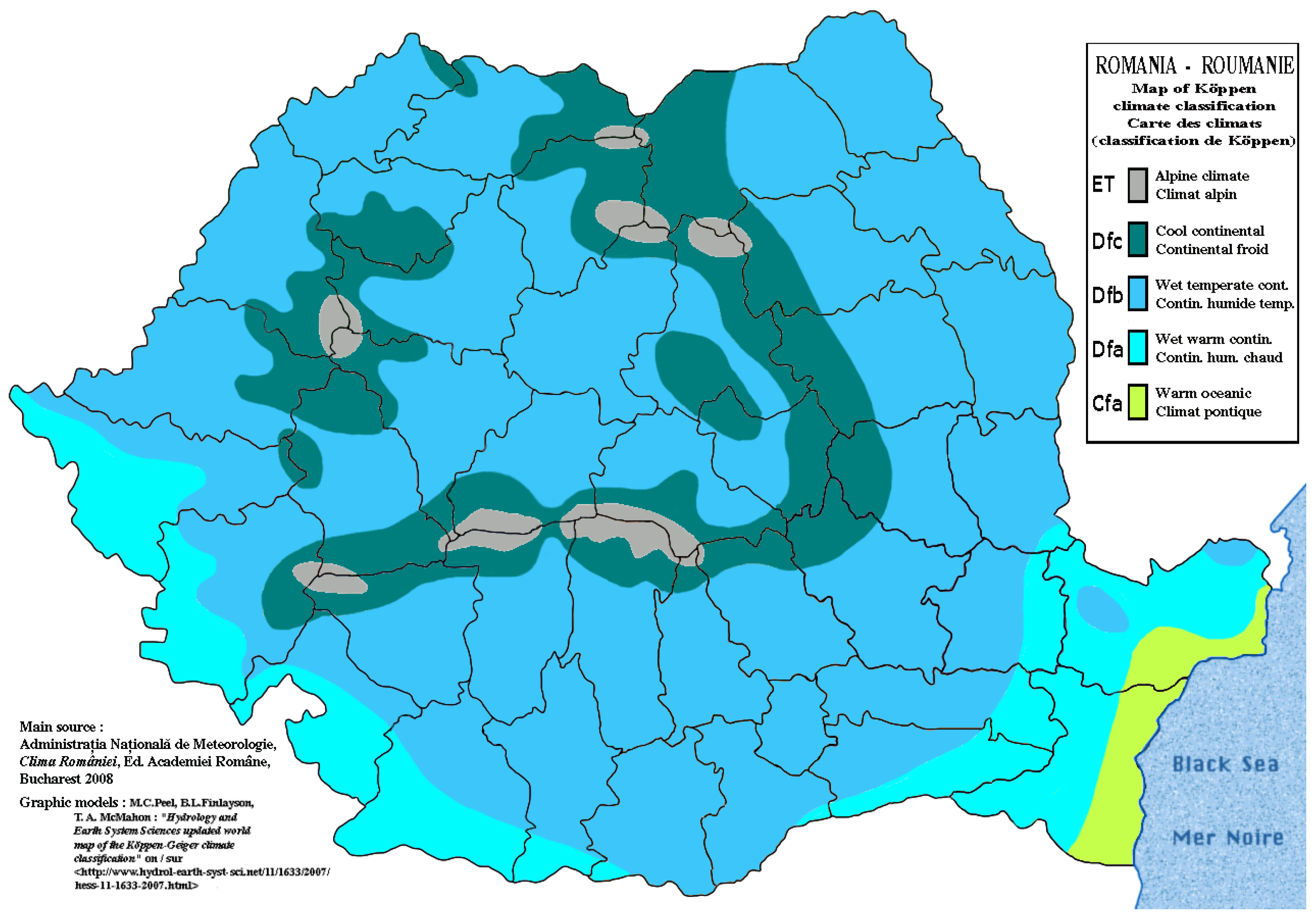
Figure 2.
IDF regionalization since 1973
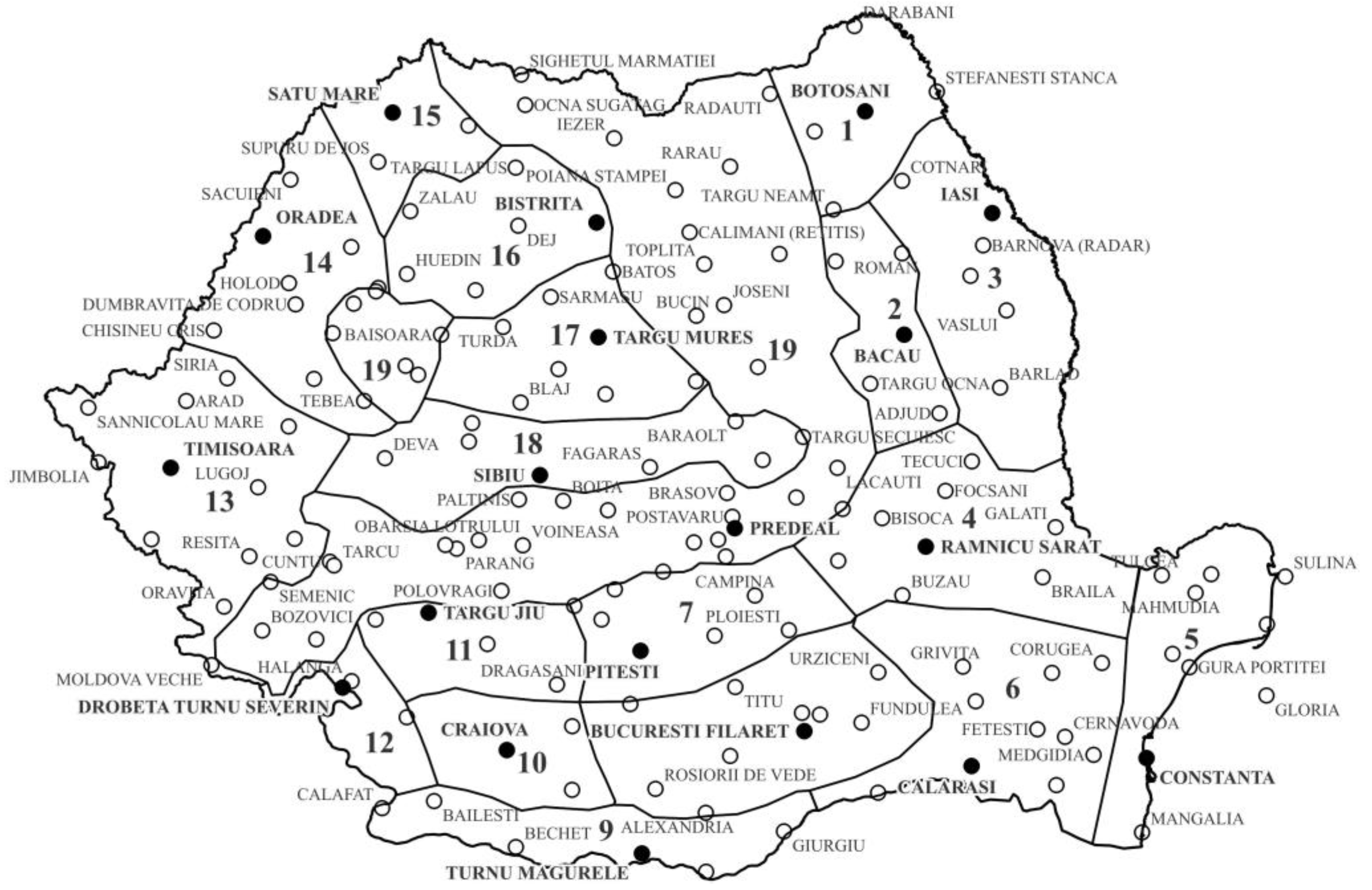
Figure 3.
Flowchart of the approach adopted.
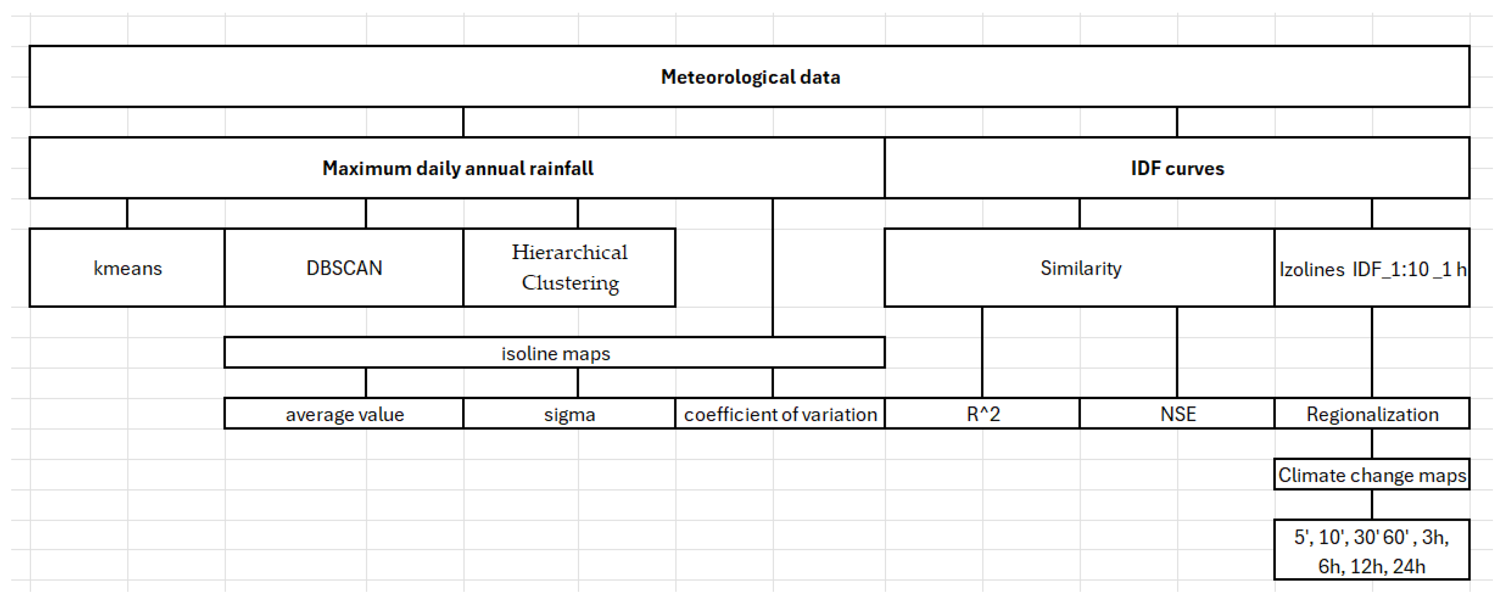
Figure 4.
Spatial distribution of meteorological stations across Romania, colored according to the coefficient of variation.
Figure 4.
Spatial distribution of meteorological stations across Romania, colored according to the coefficient of variation.
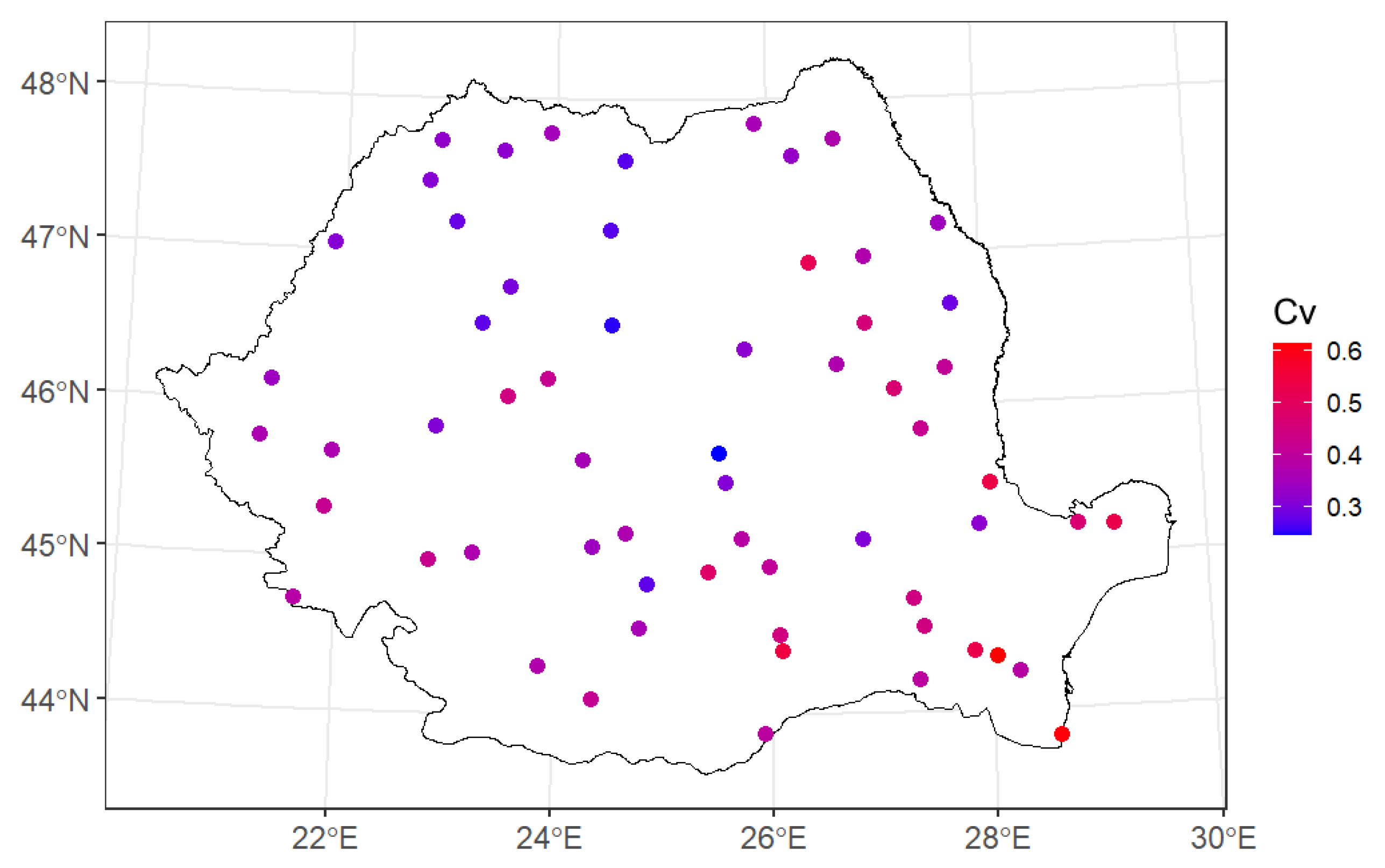
Figure 5.
Methods for determining the optimal number of clusters: (a) Elbow method (WSS); (b) Gap statistic.
Figure 5.
Methods for determining the optimal number of clusters: (a) Elbow method (WSS); (b) Gap statistic.
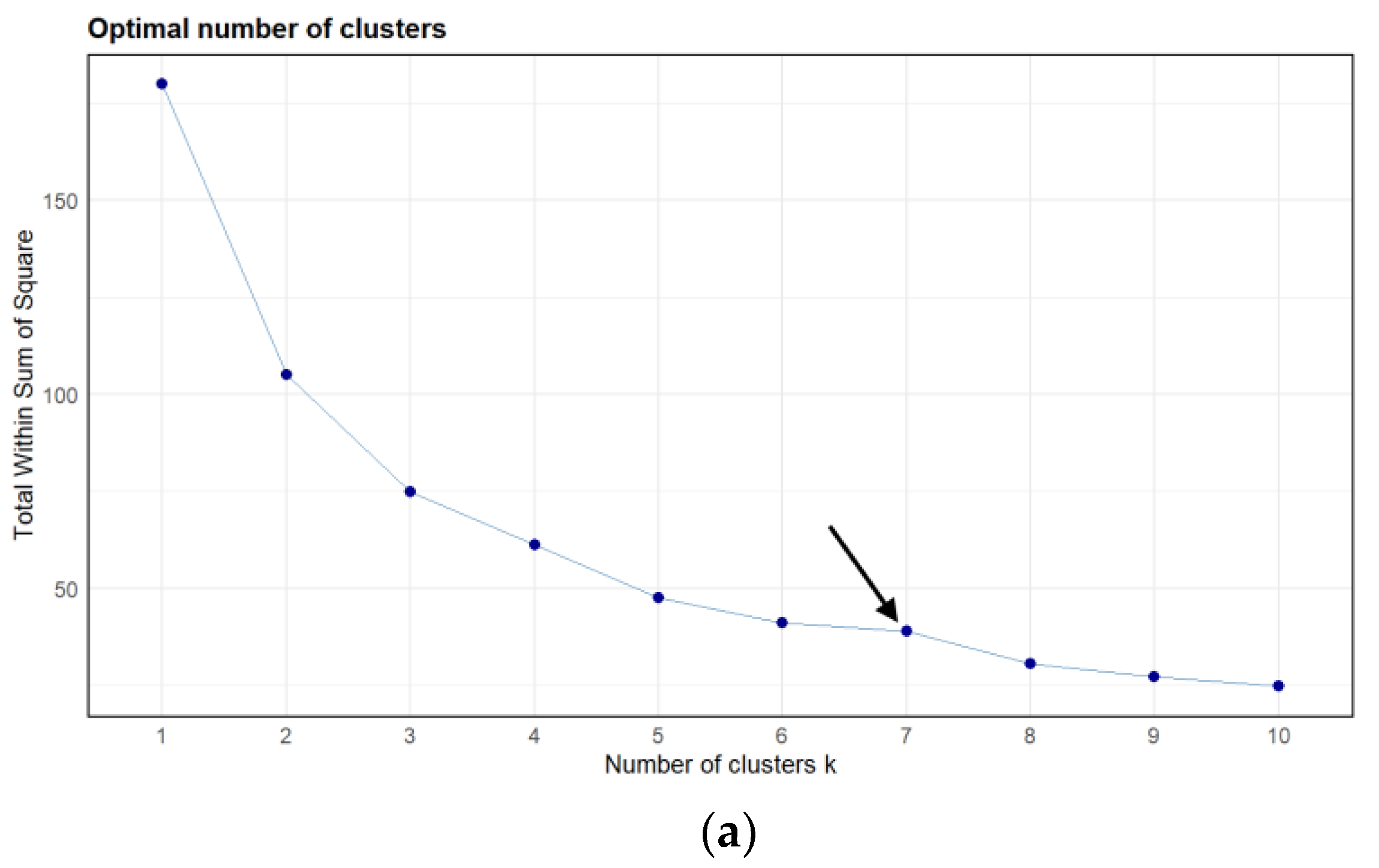
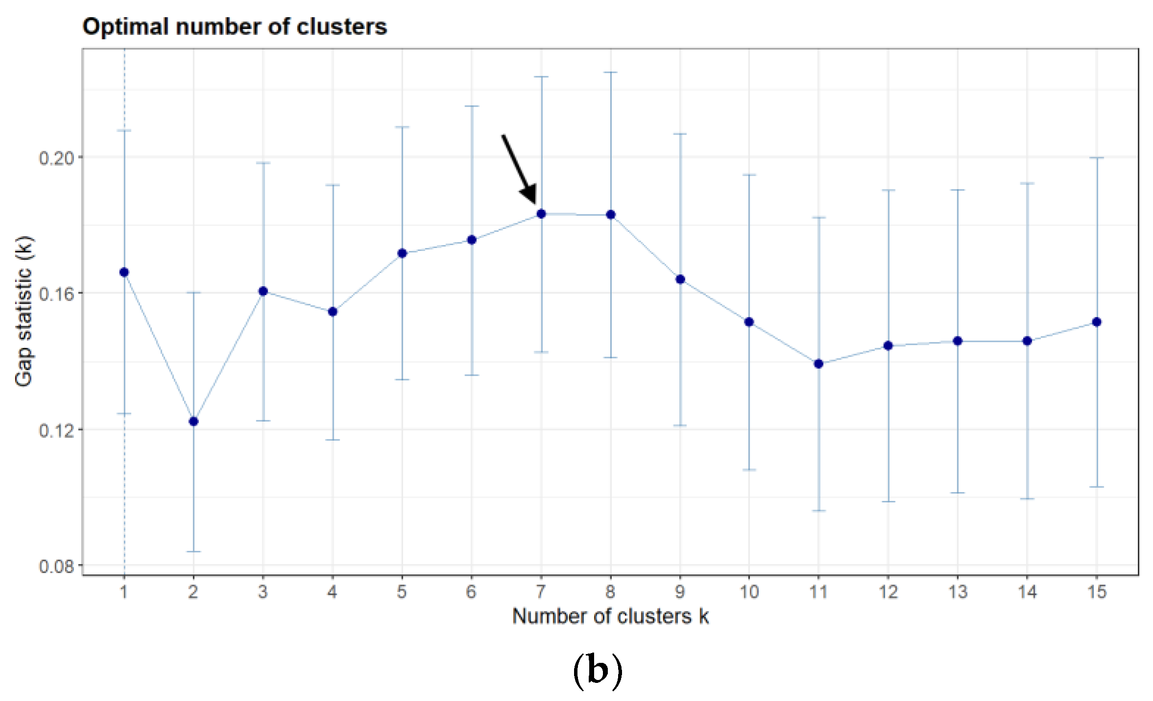
Figure 6.
Silhouette plot for k-means clustering (k = 7).
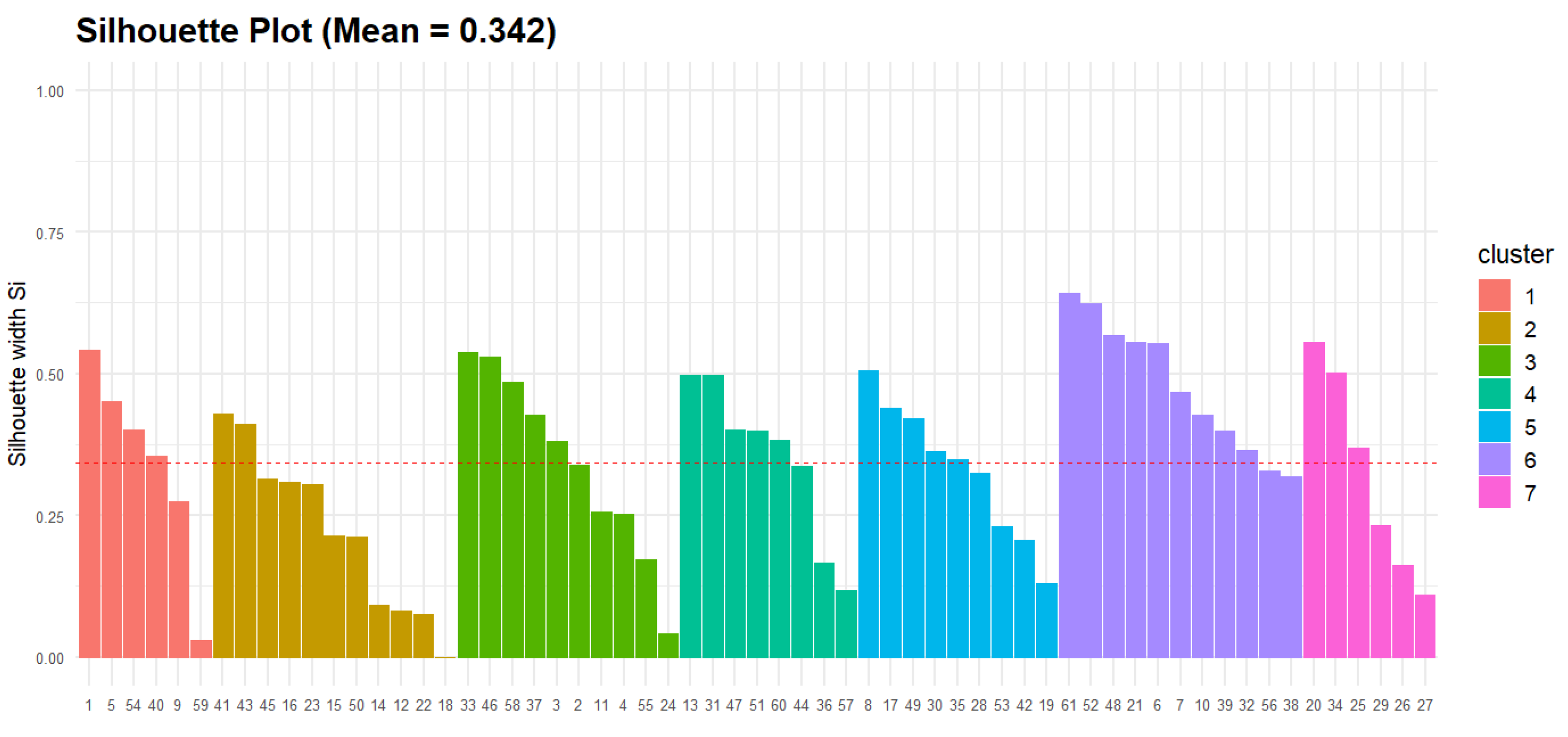
Figure 7.
k-means clustering results (k = 7) with convex hulls and cluster assignments.
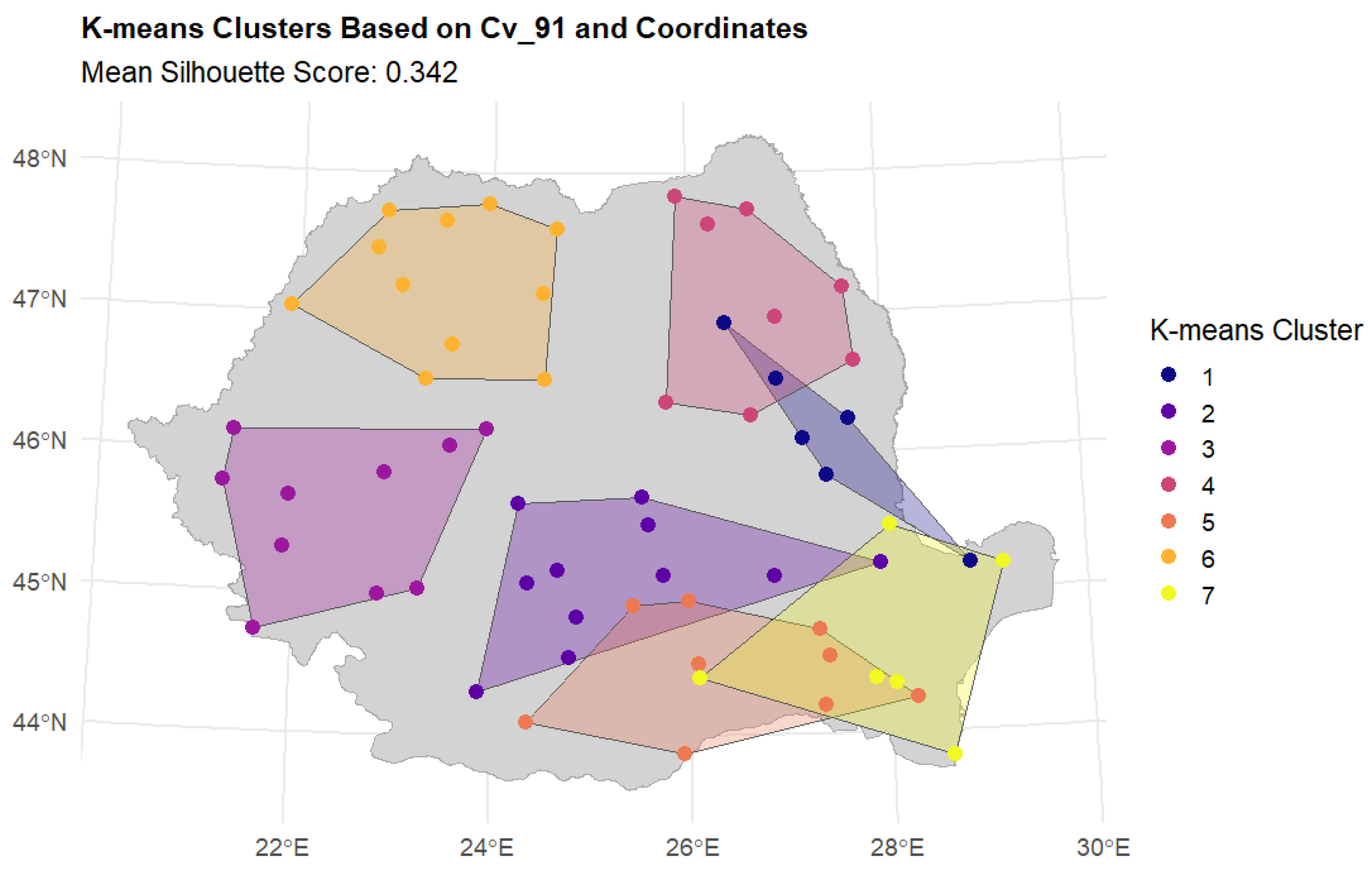
Figure 8.
Hierarchical clustering dendrogram (Ward’s method) of the stations based on Cv and station coordinates.
Figure 8.
Hierarchical clustering dendrogram (Ward’s method) of the stations based on Cv and station coordinates.

Figure 9.
The Gap Statistical plot illustrates the optimal number of clusters.
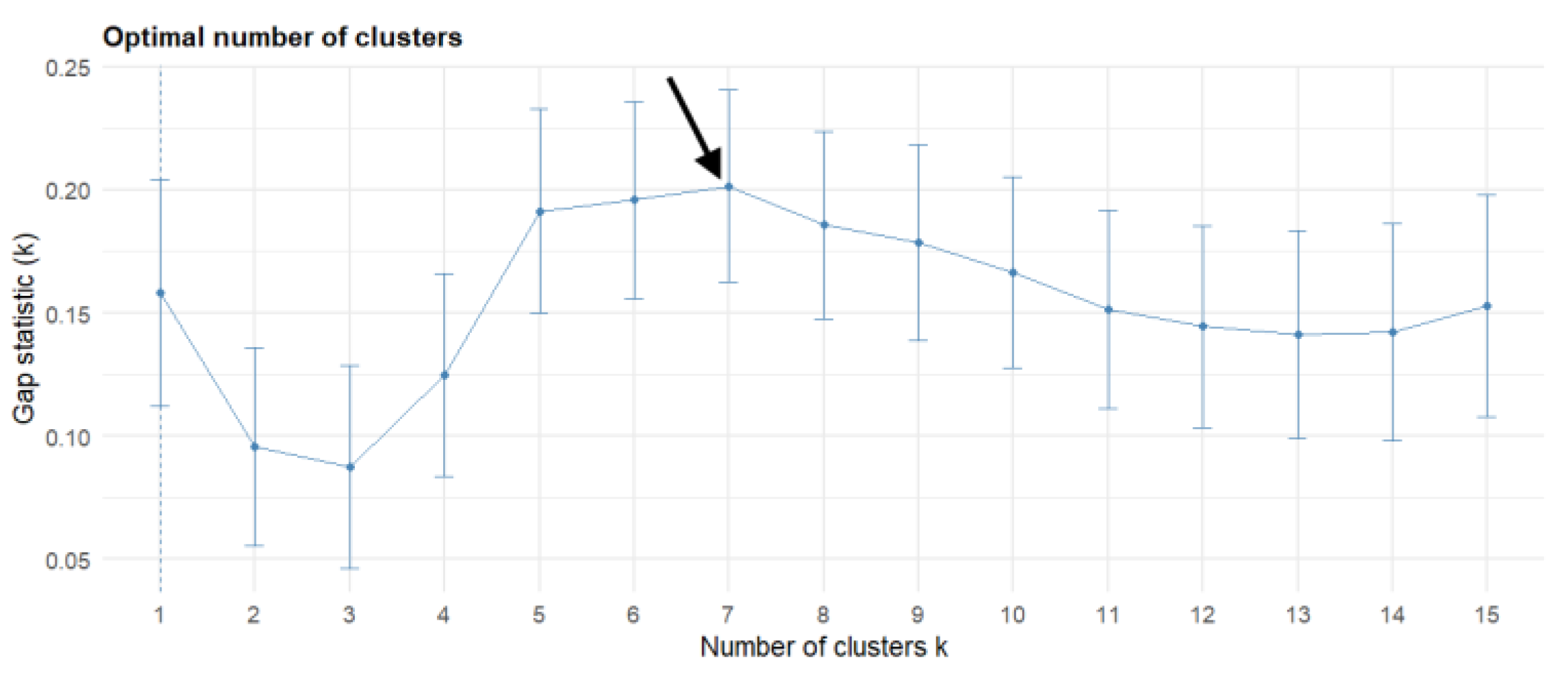
Figure 10.
Silhouette plot for hierarchical clustering (k = 7).
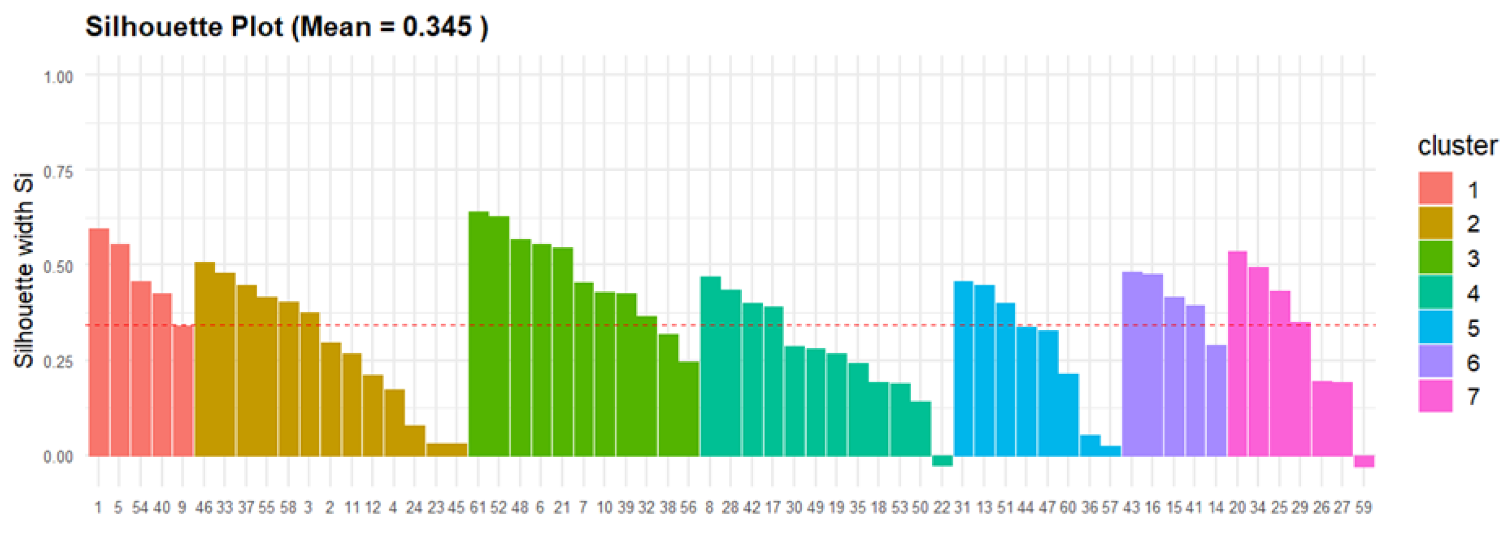
Figure 11.
Hierarchical clusters (k = 7) overlaid with convex hulls, showing cluster boundaries and station locations.
Figure 11.
Hierarchical clusters (k = 7) overlaid with convex hulls, showing cluster boundaries and station locations.
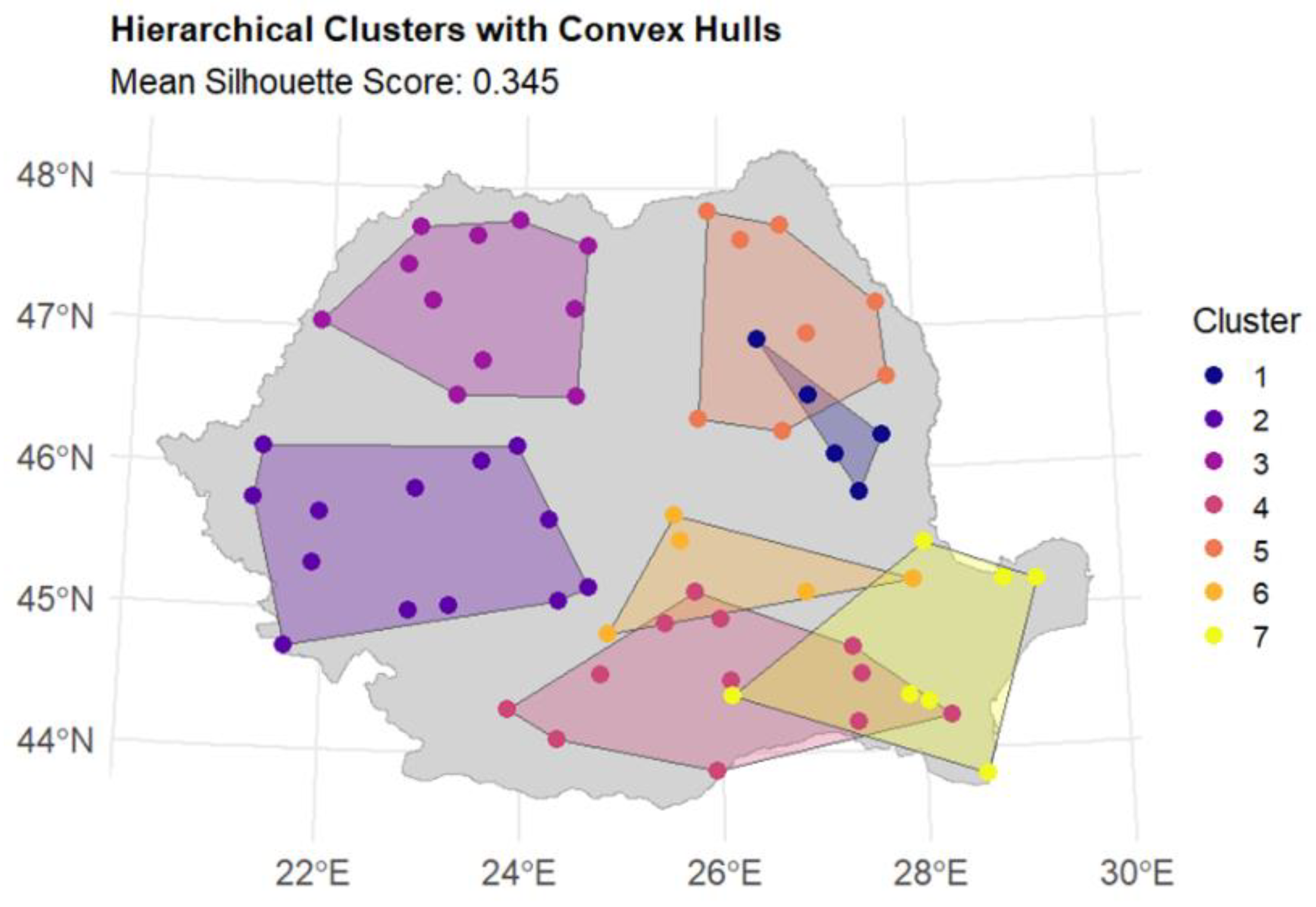
Figure 12.
Isolines of mean values.
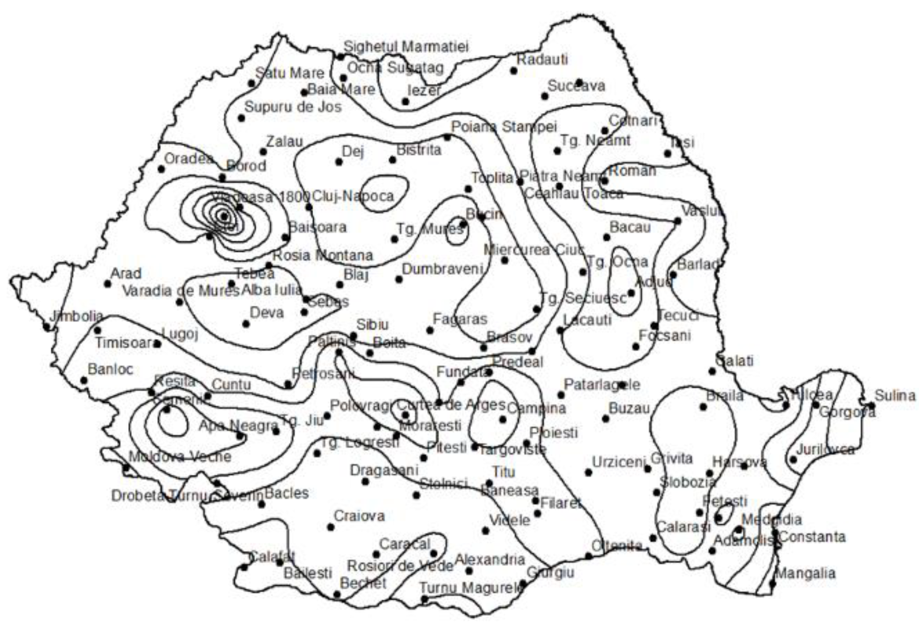
Figure 13.
Isolines of standard deviation.
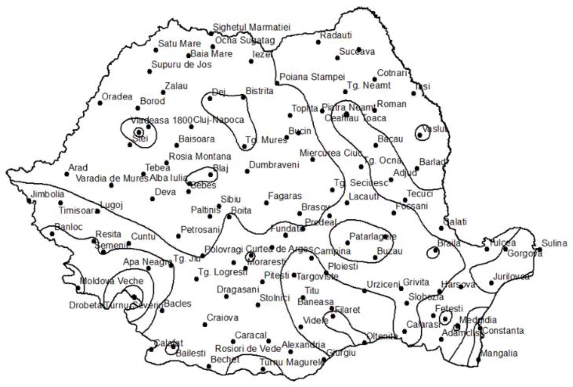
Figure 14.
Isolines of coefficient of variation.
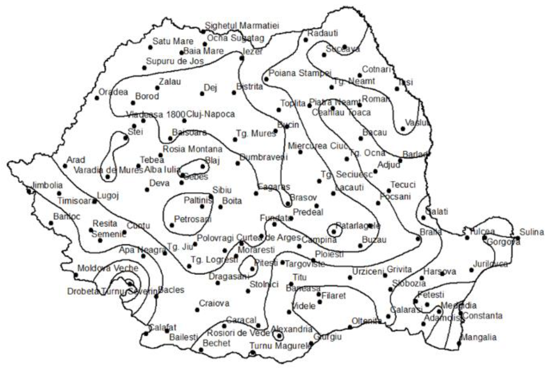
Figure 15.
Regionalization of 1-h accumulated rainfall depth for a frequency of 1:10: (a) Isolines; (b) Polygons.
Figure 15.
Regionalization of 1-h accumulated rainfall depth for a frequency of 1:10: (a) Isolines; (b) Polygons.
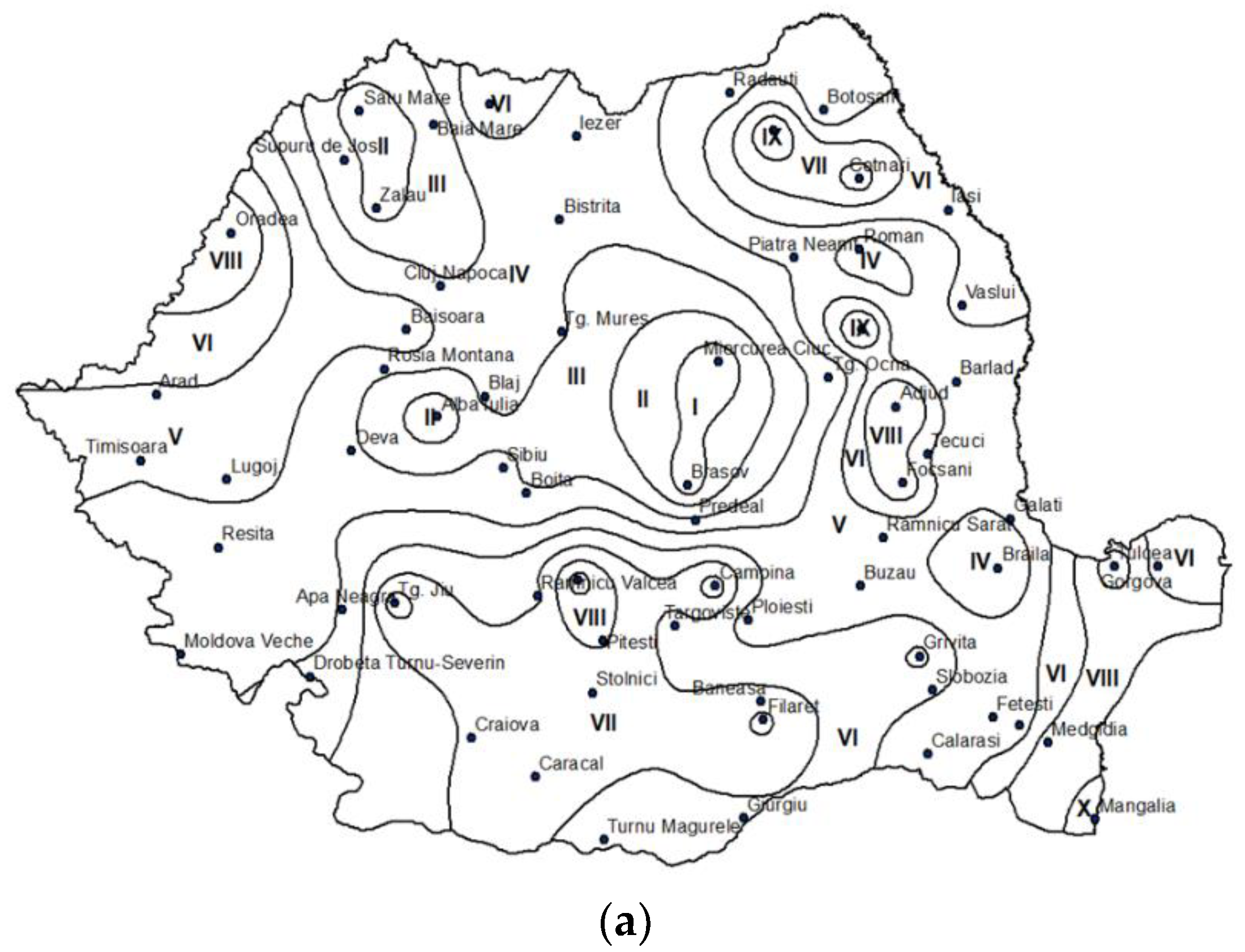
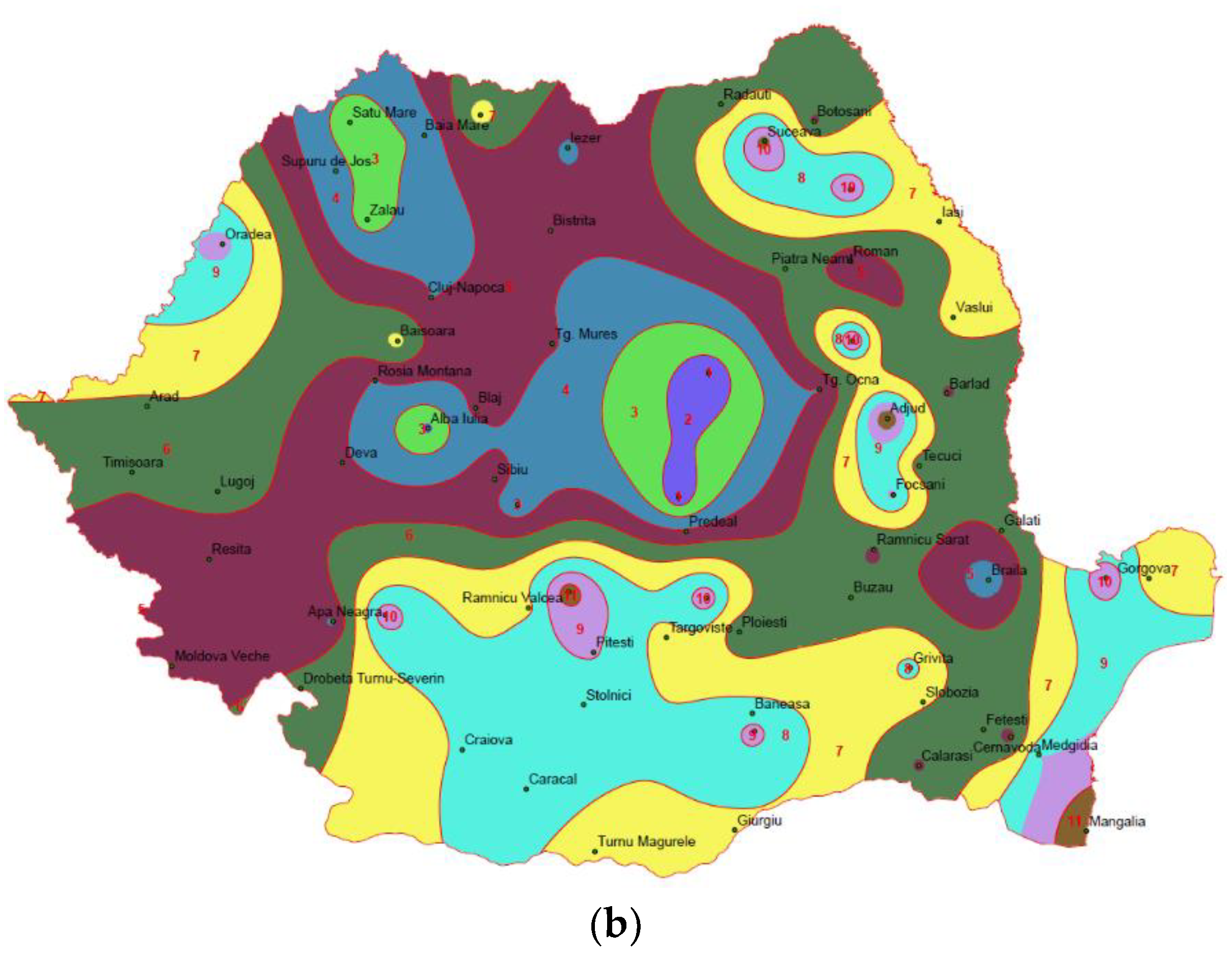
Figure 16.
Regionalization of 1-hour accumulated rainfall depth: (a) frequency 1:5; (b) frequency 1:20.
Figure 16.
Regionalization of 1-hour accumulated rainfall depth: (a) frequency 1:5; (b) frequency 1:20.
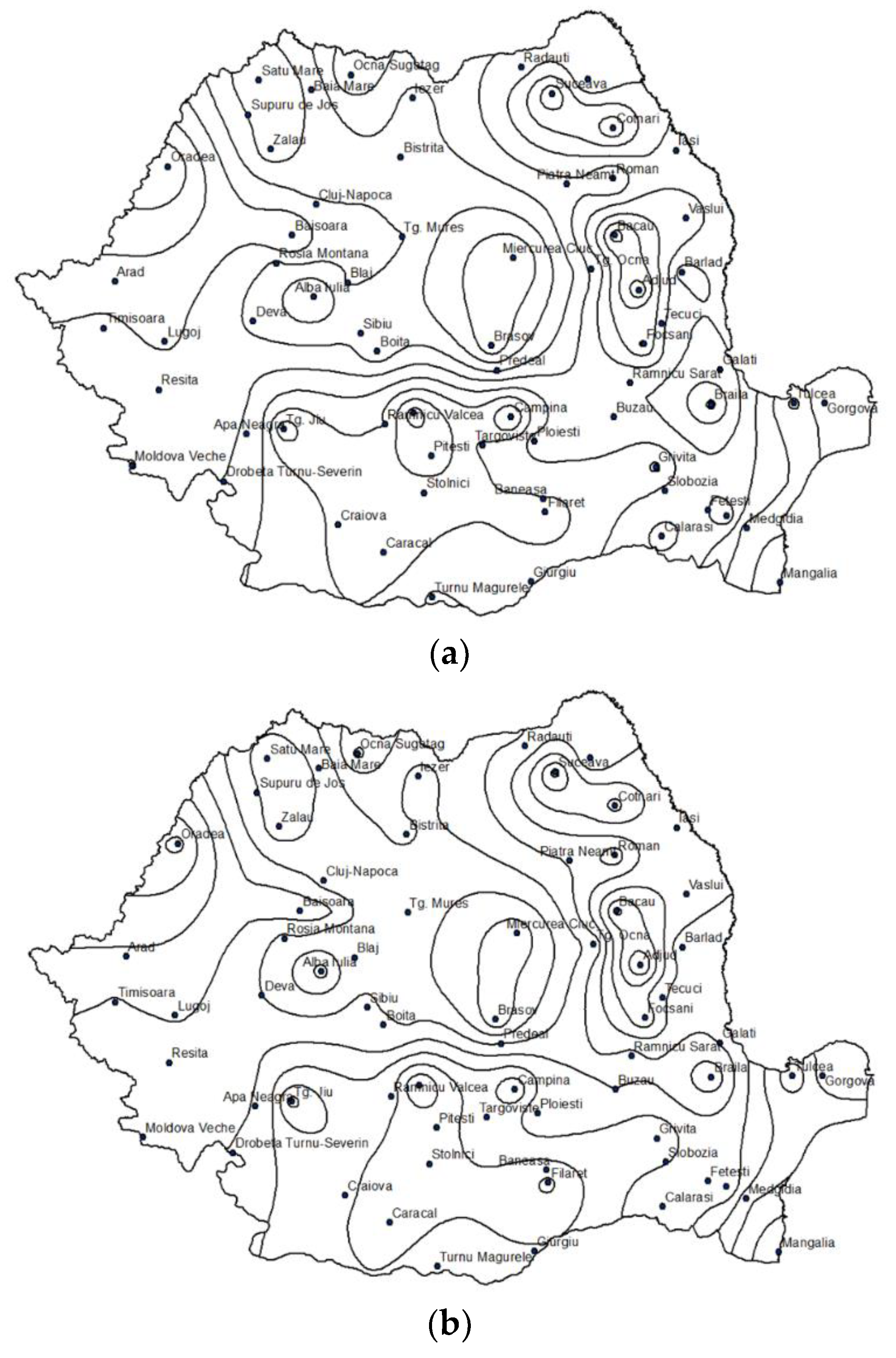
Figure 17.
Percentage differences (2025 vs. 1973) in rainfall depth by duration: (a) 5 min; (b) 10 min; (c) 30 min; (d) 60 min; (e) 180 min; (f) 360 min; (g) 720 min; (h) 1440 min.
Figure 17.
Percentage differences (2025 vs. 1973) in rainfall depth by duration: (a) 5 min; (b) 10 min; (c) 30 min; (d) 60 min; (e) 180 min; (f) 360 min; (g) 720 min; (h) 1440 min.
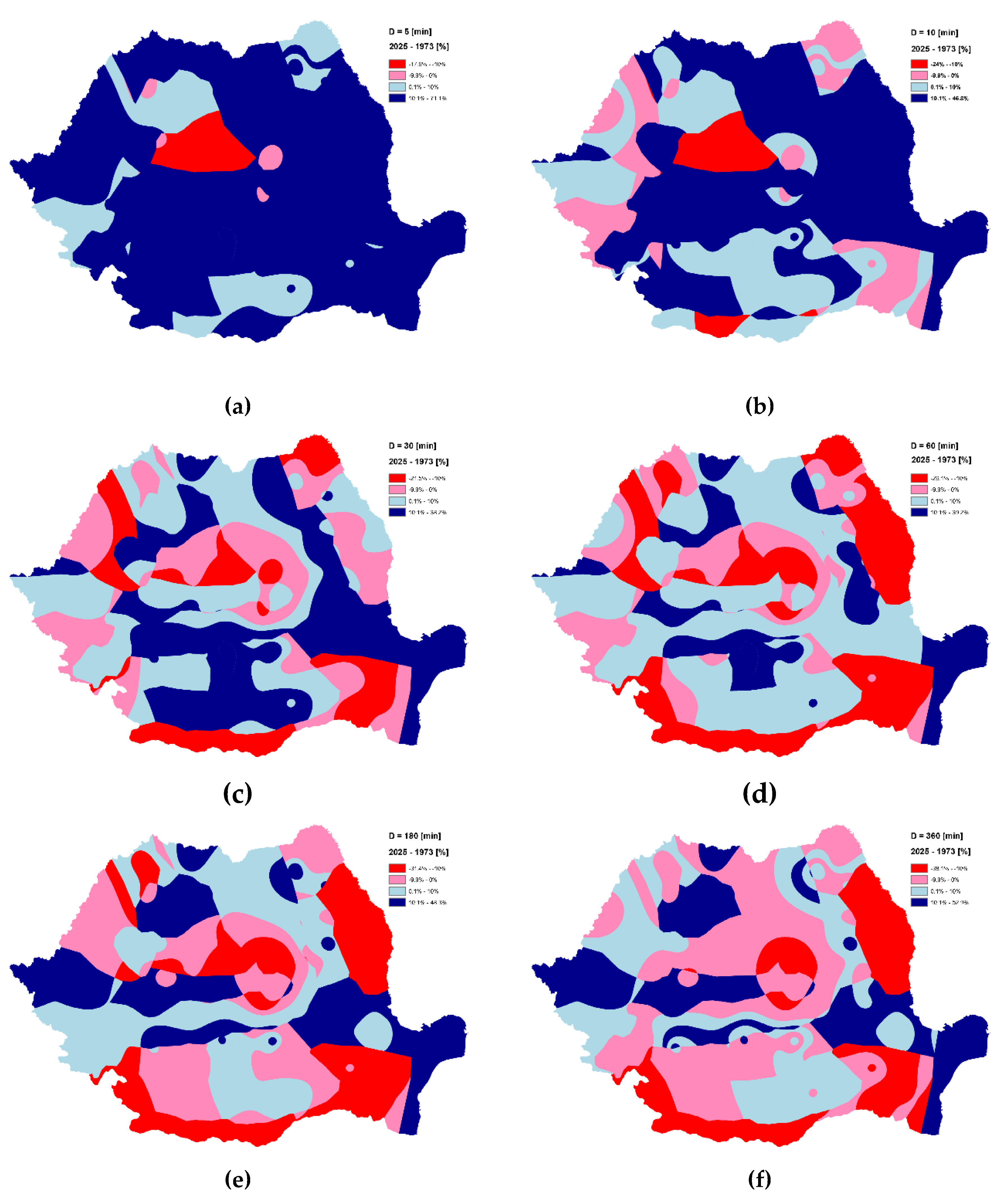
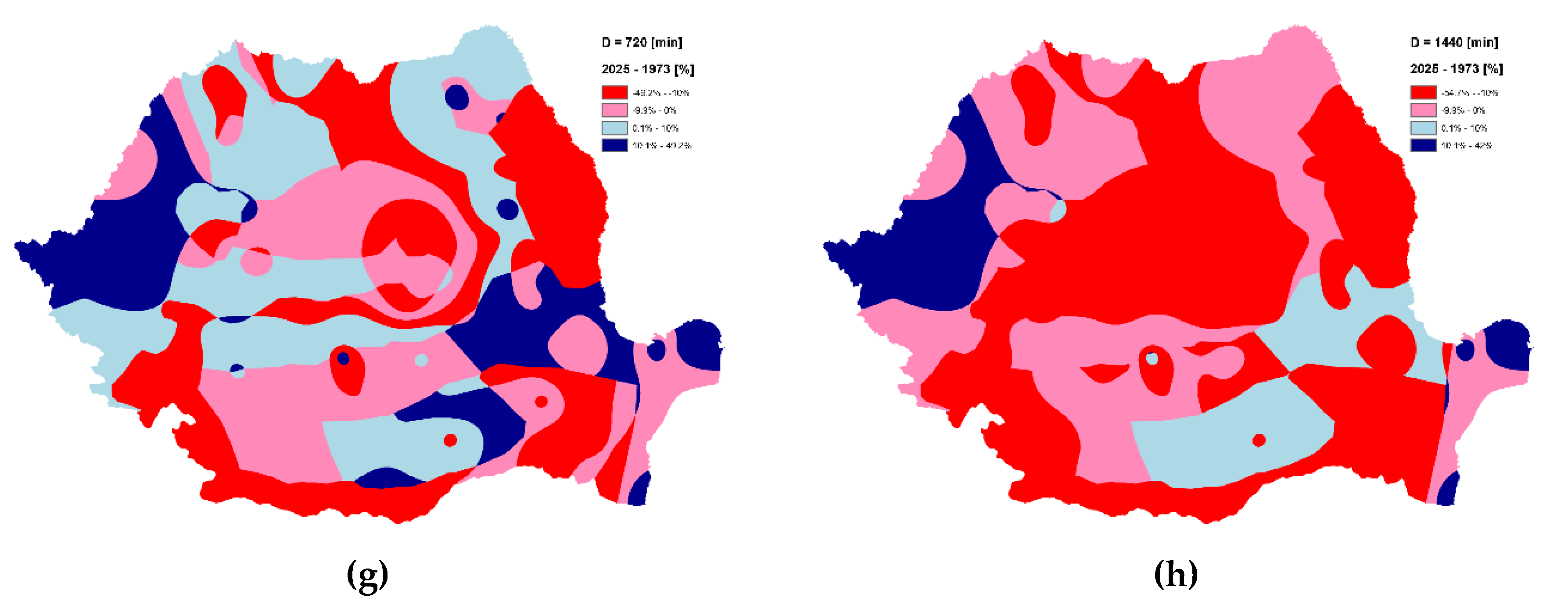
Figure 13.
Graphs of coefficients a, b and c: (a), (b), (c) − zone 1; (d), (e), (f) − zone 7; (g), (h), (i) − zone 8; (j), (k), (l) − zone 10; (a), (d), (g), (j) − a graphs; (b), (e), (h), (k) − b graphs; (c), (f), (i), (l) − c graphs; .
Figure 13.
Graphs of coefficients a, b and c: (a), (b), (c) − zone 1; (d), (e), (f) − zone 7; (g), (h), (i) − zone 8; (j), (k), (l) − zone 10; (a), (d), (g), (j) − a graphs; (b), (e), (h), (k) − b graphs; (c), (f), (i), (l) − c graphs; .
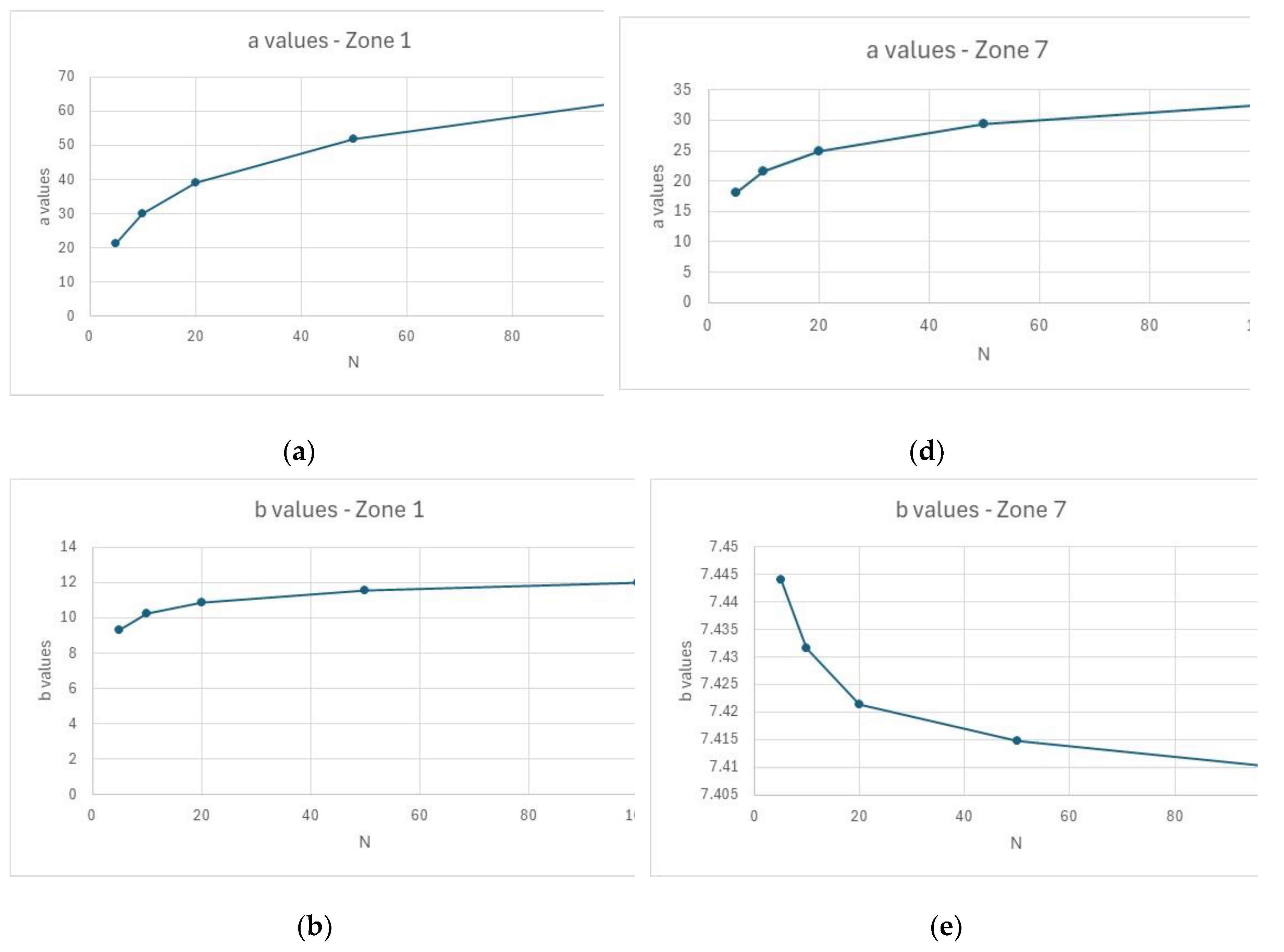
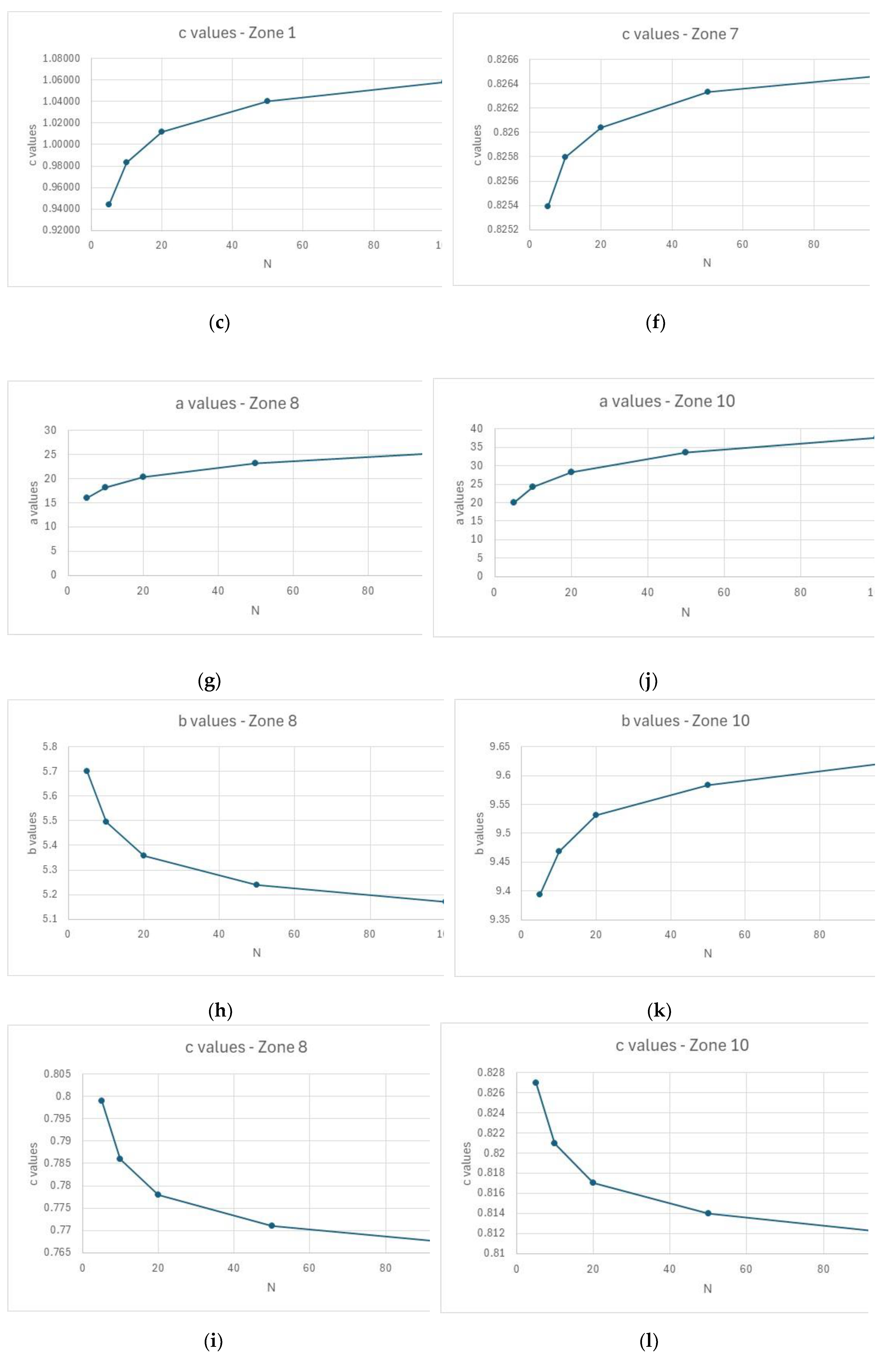
Figure 14.
IDF curves for frequency 1:10 : (a) - zone 4; (b) – zone 5.
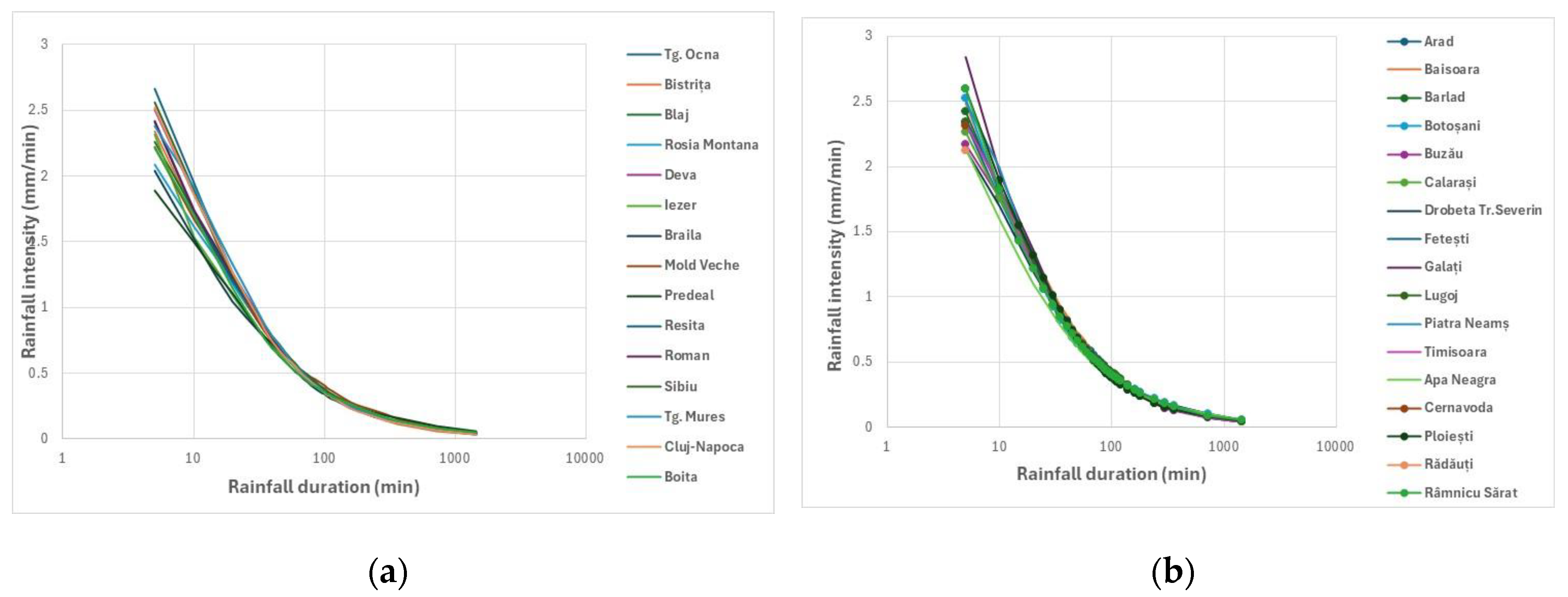
Figure 15.
Representative IDF curves for the ten homogeneous areas.
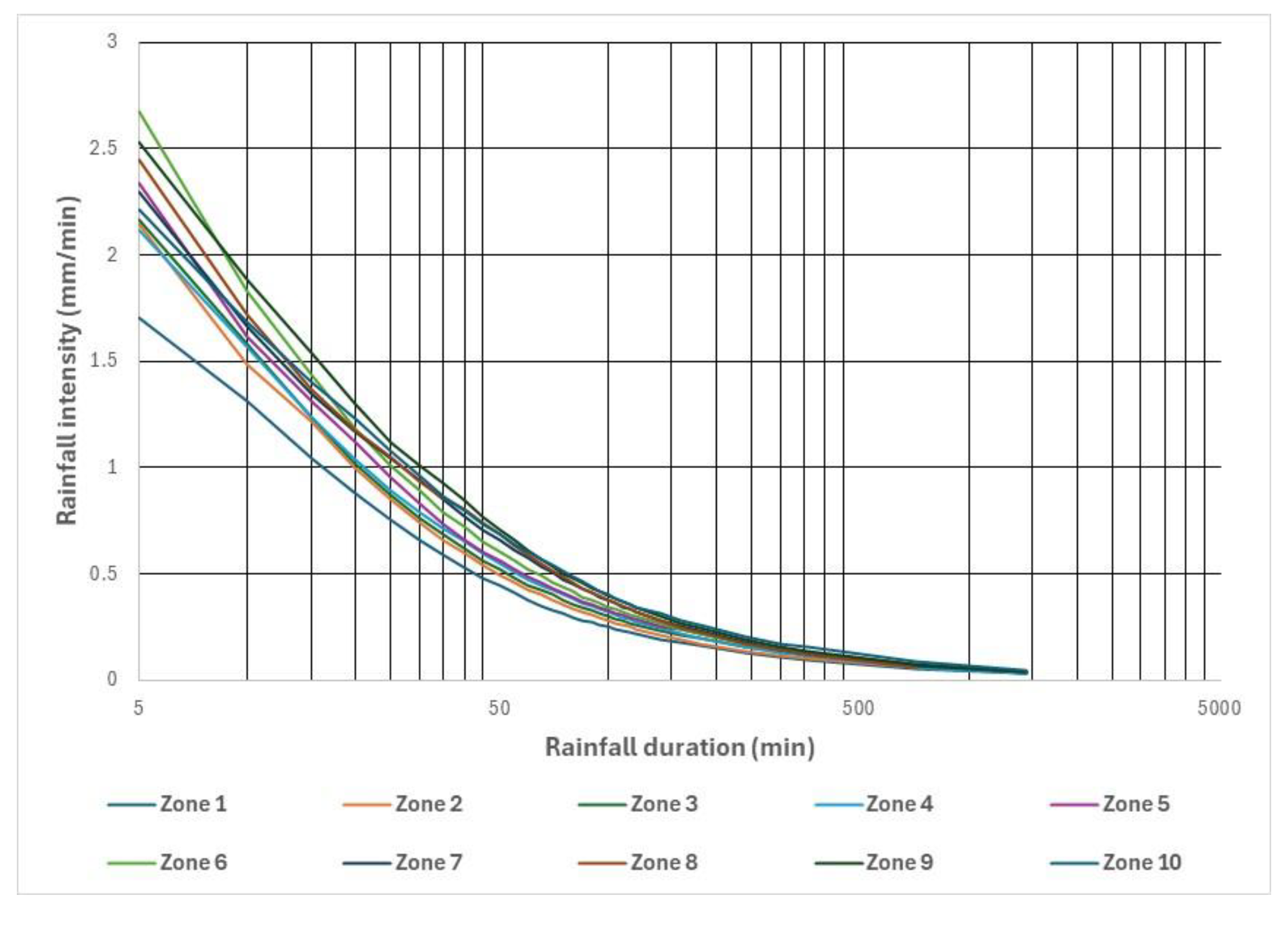
Figure 14.
IDF curve and the upper limit of its confidence interval at Filaret station.
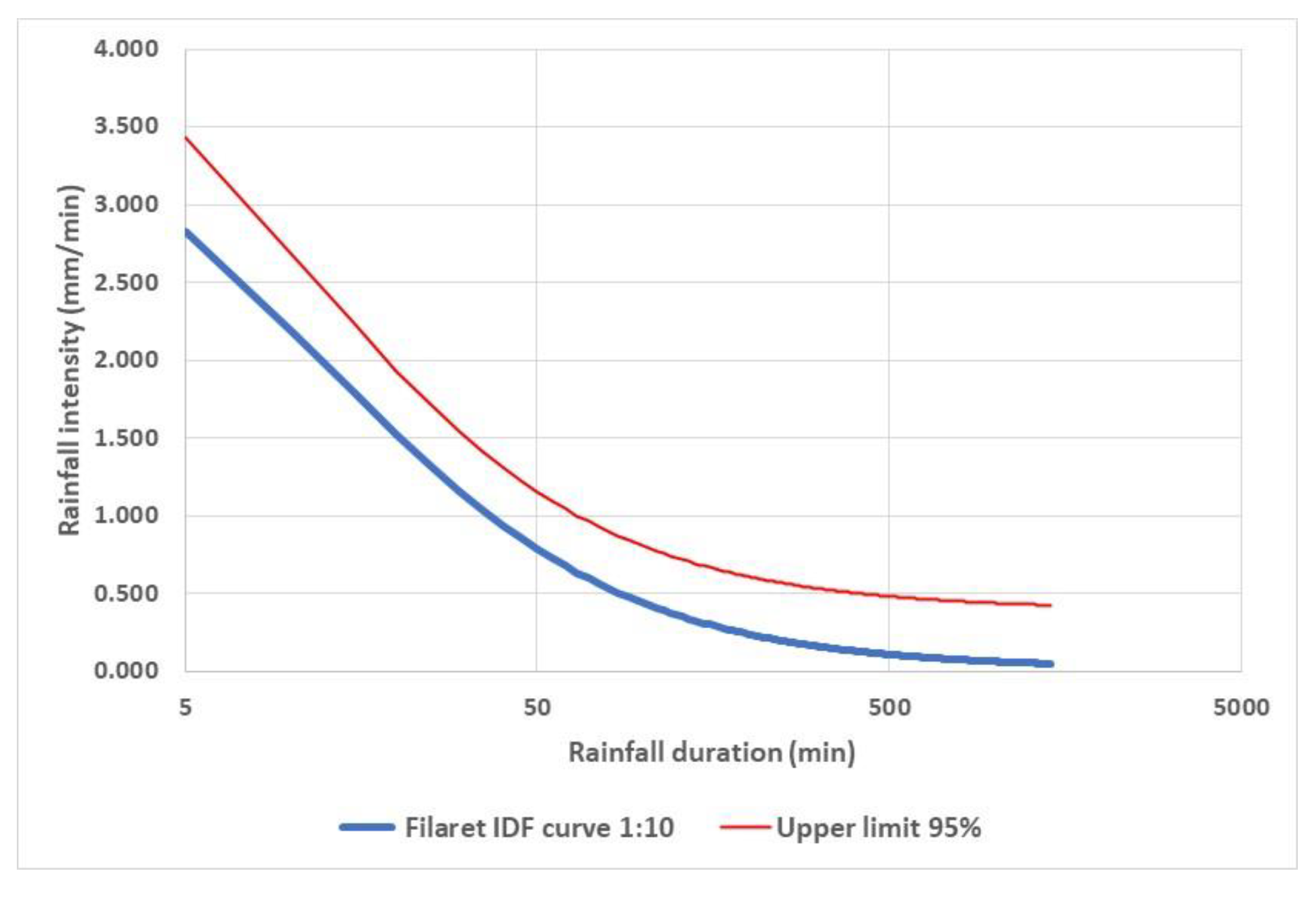
Table 1.
Design frequencies recommended in the EU standard EN 752-2.
|
Design storm frequency 1 (1 in “n ” years) |
Location |
Design flooding frequency (1 in “n ” years ) |
| 1:1 | Rural areas | 1:10 |
| 1:2 | Residential areas | 1:20 |
| City centers, industrial/commercial areas | ||
| 1:2 | - with flooding check | 1:30 |
| 1:5 | - without flooding check | - |
| 1:10 | Underground railway/ underpasses | 1:50 |
1 For design storms no surcharge shall occur.
Table 2.
NSE coefficients for a few randomly selected stations.
| Station | Station | NSE | Distance (km) |
| Arad | Turnu Măgurele 1 | 0.998964 | 387.3 |
| Lugoj | 0.997717 | 69.62 | |
| Timișoara | 0.997184 | 49.48 | |
| Fetești 1 | 0.996895 | 546.98 | |
| Bârlad 1 | 0.996293 | 488.40 | |
| Călărași 1 | 0.996179 | 517.82 | |
| Bârlad | Timișoara 1 | 0.997894 | 501.07 |
| Deva 1 | 0.99780 | 368.00 | |
| Fetești 1 | 0.997723 | 206.34 | |
| Lugoj 1 | 0.996971 | 450.42 | |
| Roman | 0.996583 | 93.51 | |
| Sibiu 1 | 0.996486 | 273.08 | |
| Blaj | Reșița | 0.996858 | 184.99 |
| Cernavoda 1 | 0.996398 | 382.33 | |
| Roman 1 | 0.996066 | 245.34 | |
| Moldova Veche | 0.995229 | 238.97 | |
| Călărași | 0.995084 | 346.32 | |
| Lugoj | Turnu Măgurele 1 | 0.998139 | 319.84 |
| Timișoara | 0.998116 | 51,61 | |
| Vaslui 1 | 0.993912 | 371,58 | |
| Târgu Mureș | 0.993226 | 225.84 | |
| Piatra Neamț 1 | 0.992969 | 370.17 | |
| Sibiu | 0.992005 | 176,41 |
1 Tables Very large distance between stations and .
Table 7.
Safety factors for urban flood risk management.
| No. | Building importance category1 | Safety coefficients |
| 1 | Exceptional | 1.20 |
| 2 | Special | 1.10 |
| 3 | Common | 1.05 |
| 4 | Reduced importance | 1.00 |
1 According to [57].
Disclaimer/Publisher’s Note: The statements, opinions and data contained in all publications are solely those of the individual author(s) and contributor(s) and not of MDPI and/or the editor(s). MDPI and/or the editor(s) disclaim responsibility for any injury to people or property resulting from any ideas, methods, instructions or products referred to in the content. |
© 2025 by the authors. Licensee MDPI, Basel, Switzerland. This article is an open access article distributed under the terms and conditions of the Creative Commons Attribution (CC BY) license (http://creativecommons.org/licenses/by/4.0/).
Copyright: This open access article is published under a Creative Commons CC BY 4.0 license, which permit the free download, distribution, and reuse, provided that the author and preprint are cited in any reuse.


