A New Electro-Gravity Theory of a Spinning Electron, and Fundamental Origin of Quantum Concepts

1. Introduction

The electron is the most fundamental charged particle of nature [1], carrying the smallest mass among all known charged particles, and is classified as a lepton in the standard model of particle physics [2,3]. It plays a fundamental role in our everyday nature as a basic building block of all chemical elements, which consist of one or more electrons orbiting in different spatial forms around an oppositely charged, massive central nucleus [4,5]. Different physical parameters of the electron - its charge, mass, as well as the spin angular momentum and the magnetic moment [6,7,8]- have been measured in great precision. The electron’s characteristics in an electromagnetic field have also been successfully modeled using quantum mechanical wave functions [9,10,11] and quantum electro-dynamics [12]. However, any internal structure of the electron, and the physical origins of its charge, mass and spin angular momentum, as well as of its associated quantum-mechanical wave function, remain mysterious. The electron is sometimes considered to be a “point particle” with no particular internal structure [13]. However, the electromagnetic energy, or its equivalent mass, for the point-particle would be infinite [14], which is unphysical and inconsistent with the finite measured mass of the electron [6]. The angular momentum, defined as the product of a rotational momentum and radius of the rotation, would also be zero for the point-particle, which is inconsistent with the non-zero measured value of the spin angular momentum of the electron. Further, the question of how the electronic charge could withstand the repulsive force due to its own electric field [14], which is infinite for the point-structure with a zero radius (or even a finite value if the electron had a non-zero radius), can not be properly answered.

In this paper, we present a new theory, referred to as a Unified Electro-Gravity (UEG) theory, which proposes to modify the concept of gravity in the presence of an electromagnetic field. In its most basic form, the proposed UEG theory introduces a new gravitational field, referred to as a UEG field, proportional to the energy density in the electromagnetic field, with the parameter of proportionality $\gamma$ referred to as the UEG constant. The proposed theory, introduced first to self-consistently model a stable structure for a static electronic charge, referred to as a static UEG electron [15,16], is then expanded as well to model a complete structure of a spinning electron.

The permittivity of the “free-space” surrounding a static UEG electron, which is conventionally assumed to be a fixed constant ${ϵ}_0$ in the Coulomb’s law or Gauss’ law, now needs to be modeled as a functional distribution ${ϵ}_0{ϵ}_r\left(r\right)$, dependent on the distribution of the new UEG field, produced due to the energy density of the electric field surrounding the static electron. The spatial variation of the permittivity function $ϵ\left(r\right)={ϵ}_0{ϵ}_r\left(r\right)$ is to be modeled consistent with the Newton’s law of gravity, with the gravitational field required to be directly proportional to the gradient of the inverse-permittivity function $1/ϵ\left(r\right)$. The resulting electrostatic field is recognized as non-linear field, where the permittivity distribution is a general function of the source charge, or equivalently the electric field is a non-linear function of the source charge. Under this non-linear condition, the definition of energy density and its expression in terms of the source charge or the electric field, used in conventional electromagnetic theory, may have to be properly modified. The electrostatic field of the static electron, properly modeled in this non-linear environment, would lead to a stable structure for the static UEG electron, with a spherical surface-charge distribution at a non-zero radius $r_e$. For the particular charge radius, the gravitational attraction due to the new UEG field maybe interpreted to balance the electrostatic self repulsion of the electronic charge, resulting in the stable structure of the static UEG electron.

A complete structure of a spinning electron may then be conceived, where the static UEG electron physically moves (spins) with a suitable rotational speed, at a certain radial distance $r_0$, to produce the known spin angular momentum $\hslash /2$ of the electron. The central acceleration of the spinning electron would be supported by suitable new UEG fields, produced due to the energy density of the surrounding electric and magnetic fields of the spinning electron. It maybe noted, the spinning electron would be self-supported by the radial forces due to the electron’s own UEG fields, in distinct contrast with orbiting of an electron around the nucleus of an atom, which instead is externally supported by the radial forces due the electric field of the central nucleus. The relative-permittivity function ${ϵ}_r\left(r\right)$ of the static UEG electron, would transform into a space-time-dependent relative-permittivity function ${ϵ}_r(r,t)$ for the spinning electron, which would be equivalent to having a space-time ripple, representing a quantum mechanical wave function. The spinning radius, speed, associated wave frequency, angular momentum, energy/mass may be modeled by extending the UEG theory of the static electron, by including additional dynamic UEG effects due to the magnetic field and field momentum-distribution of the spinning electron.

A rigorous, dynamic version of the UEG theory of the static electron would be needed to fully model the spinning electron, which maybe premature at this point. In the absence of the rigorous dynamic UEG theory, we will use suitable extension of the basic static UEG theory. The extended model, referred to as the “quasi-static” UEG model, will be guided by existing concepts from Newtonian mechanics and gravity [17], relativistic mechanics [18], electromagnetics [19] and general relativity [20], and build upon the basic principles of the static UEG theory. The objective is to explain different quantum-mechanical and quantum-electrodynamic concepts and parameters, such as the wave function [9], Planck’s constant [21] and angular momentum [11], fine structure constant [22,23] and g-factor [24], in terms of UEG concepts and parameters such as the permittivity function, the UEG constant(s) and different UEG forces. Further extension of the principles of the quasi-static UEG model of the spinning electron may physically explain energy and frequency shift in an electrodynamic scattering process, charge quantization linked to quantization of the angular momentum, and wave-particle duality based on a pilot-wave concept.

The sequence of presentation in different sections maybe outlined as follows:

Section 2 presents a basic UEG theory of the stable structure of a static electron. A fundamental dimensionless constant, relating the mass of the static UEG electron, its classical radius and the UEG constant $\gamma$ introduced in the theory, is deduced which is seen to be closely related to the fine structure constant. This is the essential part of the original modeling of a UEG static electron in [15,16], presented here for theoretical completeness and continuity with the following analysis of a spinning electron.

Section 3 presents the basic model of a spinning electron, in equivalence to an orbiting electron, and extracts basic relations between the mass of the static UEG electron, the total mass of the spinning electron, the electron g-factor and the spin angular momentum.

This is followed in Section 4 by identifying different UEG forces in a spinning electron, and formulating the total UEG acceleration that would support the spinning motion, based on first-order estimates. This would allow relating the fine structure constant from quantum electrodynamics to the UEG constant in Section 5, in an approximate form, that can be verified with a similar relationship from the static UEG model of Section 2. A much closer evaluation is explored in subSection 5.1, with deeper insights into the UEG spin model, which may assist in future development of a rigorous UEG theory.

Section 6 models the UEGravito-Magnetic effect due to field momentum associated with the spinning motion, which is shown to cancel with the basic UEG effect due to the magnetic energy density of the spinning charge. This allowed the formulations presented in the Section 4 and Section 5 using only the UEG acceleration due to the electric energy density, in order to support the spinning motion.

Section 7 relates the quantum-mechanical wave frequency to the spinning frequency in terms of the spin velocity and the g-factor. This is based on relativistic transformation between the spinning frame and a stationary external frame. The value of the g-factor is shown to be estimated from the UEG spin model in different degrees of accuracy, as compared with its known measured value. This is to reinforce validity of the spin UEG model, and illustrate finer predictive power of the model.

Fundamental significance of the spin UEG model, and potential implications of the UEG theory to model other quantum electrodynamic concepts, are discussed in Section 8.

2. Unified Electro-Gravity Theory of a Static UEG Electron

A unified electro-gravity (UEG) theory is established based on the following basic principles:

• (a) The mass m and its associated energy $W=m{c}^2$ of a given body is assumed to be inversely proportional to the relative permittivity ${ϵ}_r$, or directly proportional to the inverse-relative permittivity ${\underline{ϵ}}_r=1/{ϵ}_r$, of the surrounding medium. This is in consistency with the energy $W={\displaystyle \frac{q^2}{8\pi ϵr_q}}$ of a spherical surface charge q of radius $r_q$, placed in a medium with permittivity $ϵ={ϵ}_0{ϵ}_r$. The ${ϵ}_0$ is the permittivity of an “ideal free-space” having an ideal unit relative permittivity ${ϵ}_r=1$, which is assumed to exist far away from any gravitating body $\overline{r}\to \infty$.

Using the above concept of mass, a gravitational force $\overline{F}\left(\overline{r}\right)$ at a given location $\overline{r}$, and its associated field ${\overline{E}}_g\left(\overline{r}\right)=\overline{F}\left(\overline{r}\right)/m_0$ defined as the gravitational force applied on a unit free-mass $m_0$, maybe modeled in terms of the gradient of the inverse-relative permittivity function ${\underline{ϵ}}_r\left(\overline{r}\right)$.

$$\begin{array}{cc}& {\overline{E}}_g={\displaystyle \frac{\overline{F}}{m_0}}={\displaystyle \frac{-\overline{\nabla }W\left(\overline{r}\right)}{m_0}}={\displaystyle \frac{-\overline{\nabla }\left[m\left(\overline{r}\right)c^2\right]}{m_0}}\\ & ={\displaystyle \frac{-\overline{\nabla }\left[m_0{\underline{ϵ}}_r\left(\overline{r}\right)c^2\right]}{m_0}}=-c^2\overline{\nabla }{\underline{ϵ}}_r\left(\overline{r}\right).\end{array}$$

(1)

(b) The gravitational field, conventionally defined by the Newton’s law of gravitation, needs to be modified by adding a new part which is a function of the energy density $W_{\tau }$ associated with an electromagnetic field at a given location. As a simple first-order approximation, the new gravitational field ${\overline{E}}_{gu}$, referred to as the UEG field, is assumed to be directly proportional to the energy density, with the proportionality constant $\gamma$ referred to as the unified electro-gravity (UEG) constant. The proposed modification would maintain the Newtonian gravitational field as the total field for an electrically-neutral massive body, in the external region where the electrical energy density is zero. It would, however, change the nature of gravitation in the internal region of the neutral body, which is assumed to consist of internal charged substructures. The modified theory maybe alternately interpreted by not modifying the Newton’s law of gravitation, but re-defining the the energy density in an electromagnetic field, such that the total energy/mass of a neutral body remain unchanged.

The modified theory will fundamentally shape the physical structure of any charged particle, such as an electron. The new electro-gravitational field would determine the inverse-relative permittivity function ${\underline{ϵ}}_r\left(\overline{r}\right)$ around an electron, as per the relation (1). We may further assume that the new gravitational field ${\overline{E}}_{gu}=-\gamma W_{\tau }\widehat{r}$, directed toward the center along $-\widehat{r}$, is much stronger than the conventional Newtonian gravitational field, and therefore would essentially be equal to the total gravitational field ${\overline{E}}_g$.

$$\begin{array}{cc}& {\overline{E}}_g=-c^2\overline{\nabla }{\underline{ϵ}}_r\left(\overline{r}\right)\simeq {\overline{E}}_{gu}=-\gamma W_{\tau }\widehat{r}.\end{array}$$

(2)

2.1. Energy Density in a Non-Linear Medium

In the above unified electro-gravity (UEG) model, the permittivity distribution of the free-space is dependent upon the energy density distribution, which is dependent upon the source charge. This is unlike a linear dielectric medium where the permittivity function is independent of the field strength or the source charge. Having the permittivity distribution to be a function of the source charge, is equivalent to having the electric field distribution to be a non-linear function of the source charge. The energy density in such a non-linear medium needs to be properly modeled, using a general expression for the energy density.

The electric field $\overline{E}$ and the electric flux density $\overline{D}$ produced due to a spherical surface charge q of radius $r_q$, at a distance r from the center of the charge, in the presence of a permittivity distribution $ϵ\left(r\right)=1/\underline{ϵ}\left(r\right)$, may be expressed using the Coulomb’s law.

$$\begin{array}{cc}& \overline{E}={\displaystyle \frac{q}{4\pi r^2ϵ\left(r\right)}}\widehat{r},\overline{D}={\displaystyle \frac{q}{4\pi r^2}}\widehat{r},\overline{E}={\displaystyle \frac{\overline{D}}{ϵ\left(r\right)}}=\underline{ϵ}\left(r\right)\overline{D}.\end{array}$$

(3)

The total energy W and the associated mass $m=W/c^2$ of the charge maybe calculated by integrating the energy density $W_{\tau }$ in its electric field over the spherical volume $\tau$ outside of the charge $r>r_q$. The electric field, and the associated energy density, in the spherical region with $r<r_q$ would be zero. The $W_{\tau }$ maybe expressed in (4) in terms of the flux density $\overline{D}=\underline{ϵ}\overline{E}$ due to the charge q, and its incremental value $d\overline{D}$ due to an incremental change $dq$ of the charge. This expression of the energy density would be valid for a general non-linear medium, which maybe simplified as $W_{\tau }=(1/2)\underline{ϵ}{\left|\overline{D}\right|}^2$ for a linear medium.

$$\begin{array}{cc}& W={\int }_{\tau }{W}_{\tau }d\tau ={\int }_{\tau }{(}_{q=0}^{q}d{W}_{\tau })d\tau =m_0{c}^2,\\ & W_{\tau }{=}_{q=0}^{q}d{W}_{\tau }{=}_{q=0}^q\underline{ϵ}\overline{D}·d\overline{D}={\displaystyle \frac{1}{2}}{\underline{ϵ}}^{\prime }{\left|\overline{D}\right|}^2,\\ & {\underline{ϵ}}^{\prime }={{\displaystyle \frac{2}{q^2}}}_{q=0}^q\underline{ϵ}\left(q\right)qdq={{\displaystyle \frac{2{\underline{ϵ}}_0}{q^2}}}_{q=0}^q{\underline{ϵ}}_r\left(q\right)qdq={\underline{ϵ}}_0{\underline{ϵ}}_r^{\prime }.\end{array}$$

(4)

In equivalency to a conventional definition of the energy density for a linear medium, it would be useful to define a new variable ${\underline{ϵ}}^{\prime }$ for a non-linear medium. The conventional expression of the energy density for a linear medium, with the inverse-permittivity $\underline{ϵ}$ for the linear medium simply substituted by the new equivalent variable ${\underline{ϵ}}^{\prime }$, would be valid as well for a non-linear medium.

Now, combining (4,3) with (2), a governing relationship for the inverse-relative permittivity function ${\underline{ϵ}}_r\left(\overline{r}\right)$ is established.

$$\begin{array}{cc}& c^2\overline{\nabla }{\underline{ϵ}}_r\left(\overline{r}\right)\simeq \gamma W_{\tau }\widehat{r}={\displaystyle \frac{\gamma \widehat{r}}{16{\pi }^2{r}^4{ϵ}_0}}\underset{0}{\overset{q}{\int }}q{\underline{ϵ}}_r(q,r)dq.\end{array}$$

(5)

2.2. Series Solution for the Inverse-Relative Permittivity Function ${\underline{ϵ}}_r\left(\overline{r}\right)$

The inverse-relative permittivity function ${\underline{ϵ}}_r\left(r\right)$ maybe solved by expanding it as power-series of $r^{-i}$ with unknown coefficients $b_i$, $i=0,1,2,\dots$, and then finding the coefficients in order to satisfy the above UEG relation (5). This would be possible by establishing an iterative process, relating a coefficient $b_i$ with an increasingly higher index i to those with a lower index, starting with the known value for the lowest coefficient $b_0$. In the limit of large distance r, the ${\underline{ϵ}}_r\left(r\right)$ would approach unity, fixing the coefficient $b_0=1$.

The governing relationship (5) for ${\underline{ϵ}}_r\left(r\right)$ would require the series solution with non-zero values of the coefficients $b_i$ only for $i=0,3,6,9,\dots$. Accordingly, the series solution for the ${\underline{ϵ}}_r\left(r\right)$ maybe conveniently expressed as a power series of a normalized variable $t={(r_{\mu }/r)}^{1.5}$, with even powers of t. $r_{\mu }$ is a suitable normalization constant to be determined from (5), which maybe shown to be proportional to ${\gamma }^{1/3}$. We need not present the detailed steps, as prescribed above, to derive the individual coefficients for the series. The final solution for ${\underline{ϵ}}_r\left(r\right)$ is expressed in (6), which may simply be substituted in (5) to verify its validity. The series (6) may be recognized as the zeroth-order Bessel function $J_0\left(t\right)$.

$$\begin{array}{cc}& {\underline{ϵ}}_r\left(r\right)\simeq 1-{\displaystyle \frac{t^2}{2^2{[1!]}^2}}+{\displaystyle \frac{t^4}{2^4{[2!]}^2}}-{\displaystyle \frac{t^6}{2^6{[3!]}^2}}+\dots ;t={(r_{\mu }/r)}^{1.5},\\ & r_{\mu }={\left({\displaystyle \frac{\gamma q^2}{24{\pi }^2{c}^2{ϵ}_0}}\right)}^{1/3}=5.14\times {10}^{-16}{\gamma }^{1/3}.\end{array}$$

(6)

Figure 1.

Figure 1.

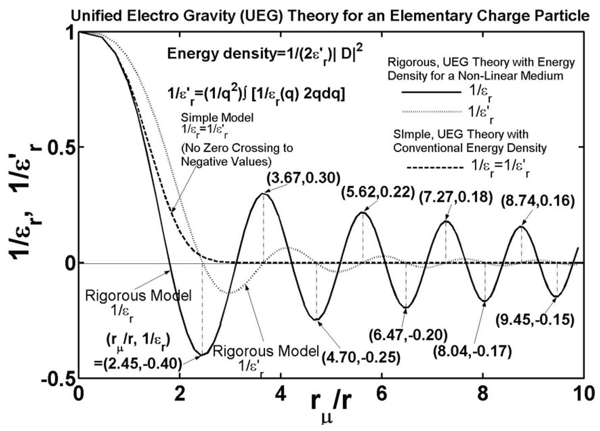
The inverse-relative permittivity function ${\underline{ϵ}}_r=1/{ϵ}_r$ of (6), as well as the corresponding effective function ${\underline{ϵ}}_r^{\prime }=1/{ϵ}_r^{\prime }$ of (7) deduced from (6) using the definition (4), are plotted in Figure 1 as a function of the normalized radius $r_{\mu }/r=t^{2/3}$. The series (7) may be recognized to be equal to $(2/t)J_1\left(t\right)$, where $J_1\left(t\right)$ is the first-order Bessel function.

$$\begin{array}{cc}& {\underline{ϵ}}_r^{\prime }\left(r\right)={\displaystyle \frac{2}{q^2}}\underset{0}{\overset{q}{\int }}q{\underline{ϵ}}_r(q,r)dq\\ & \simeq 1-{\displaystyle \frac{t^2}{2^2{[1!]}^2\times 2}}+{\displaystyle \frac{t^4}{2^4{[2!]}^2\times 3}}-{\displaystyle \frac{t^6}{2^6{[3!]}^2\times 4}}+\dots .\end{array}$$

(7)

The function ${\underline{ϵ}}_r=1/{ϵ}_r$ that would have resulted if a conventional energy density for a linear medium were used (incorrectly) in the above derivation (equations (5,4)), where the effective function ${\underline{ϵ}}_r^{\prime }=1/{ϵ}_r^{\prime }$ from (4) that defines the energy density would be equal to the function ${\underline{ϵ}}_r=1/{ϵ}_r$, is expressed in (8), and is also plotted in Figure 1 for reference.

$$\begin{array}{cc}& {\underline{ϵ}}_r\left(r\right)={\underline{ϵ}}_r^{\prime }\left(r\right)\simeq 1-{\displaystyle \frac{t^2}{2^{2}1!}}+{\displaystyle \frac{t^4}{2^{4}2!}}-{\displaystyle \frac{t^6}{2^{6}3!}}+\dots \\ & =e^{-t^2/4}.\end{array}$$

(8)

Notice in the Figure 1 that the function ${\underline{ϵ}}_r$ of (6) (and the corresponding effective function ${\underline{ϵ}}_r^{\prime }$ of (7)), derived using the rigorous definition of the energy density (4) for a non-linear medium, exhibits an oscillatory behavior changing its sign from positive to negative values and vice versa. This is in contrast with the result for ${\underline{ϵ}}_r=1/{ϵ}_r$ =${\underline{ϵ}}_r^{\prime }=1/{ϵ}_r^{\prime }$ from (8) (using a simplistic (incorrect) UEG model), which monotonically approaches zero with no oscillatory behavior. The rigorously derived, oscillatory behavior of the ${\underline{ϵ}}_r=1/{ϵ}_r$ and ${\underline{ϵ}}_r^{\prime }=1/{ϵ}_r^{\prime }$ functions is a key development, which would lead also to an oscillatory behavior of the total energy/mass of the charge particle as a function of radius, to be established in the following section. This would allow the charge particle to maintain a stable structure at discrete values of radius, where the total energy/mass of the particle would be locally minimum.

2.3. Particle Energy and Mass, as a Function of the Charge Radius

Once the inverse-relative permittivity function ${\underline{ϵ}}_r\left(r\right)$ is solved, the energy density can be expressed in terms of the ${\underline{ϵ}}_r\left(r\right)$ using (4), which can then be integrated over the total volume in the external region of a spherical surface-charge distribution (there is no field or energy in the internal region), to obtain the total energy or the equivalent mass $m=m_0$ of the particle.

$$\begin{array}{cc}& m=m_0={\displaystyle \frac{W}{c^2}}={\displaystyle \frac{1}{4\pi c^2{ϵ}_0}}\underset{r}{\overset{\infty }{\int }}{\displaystyle \frac{1}{r^2}}\underset{0}{\overset{q}{\int }}q{\underline{ϵ}}_r(q,r)dqdr\\ & =m_{\mu }\sum _{k=0}^{\infty }{\displaystyle \frac{{(-1)}^k{t}^{(2k+\frac{2}{3})}}{2^{2k}{(k!)}^2(k+1)(3k+1)}},\\ & m_{\mu }={\displaystyle \frac{q^2}{{8\pi c}^2{ϵ}_0{r}_{\mu }}}=2.49\times {10}^{-30}{\gamma }^{-1/3}.\end{array}$$

(9)

The charge radius in (9) is maintained as a general variable (=r). The general mass function $m\left(r\right)$ in (9) would also represent the equivalent energy (=$c^{2}m\left(r\right)$) contained in the field external to a sphere of radius r, produced due to the charge placed at any radius less than r.

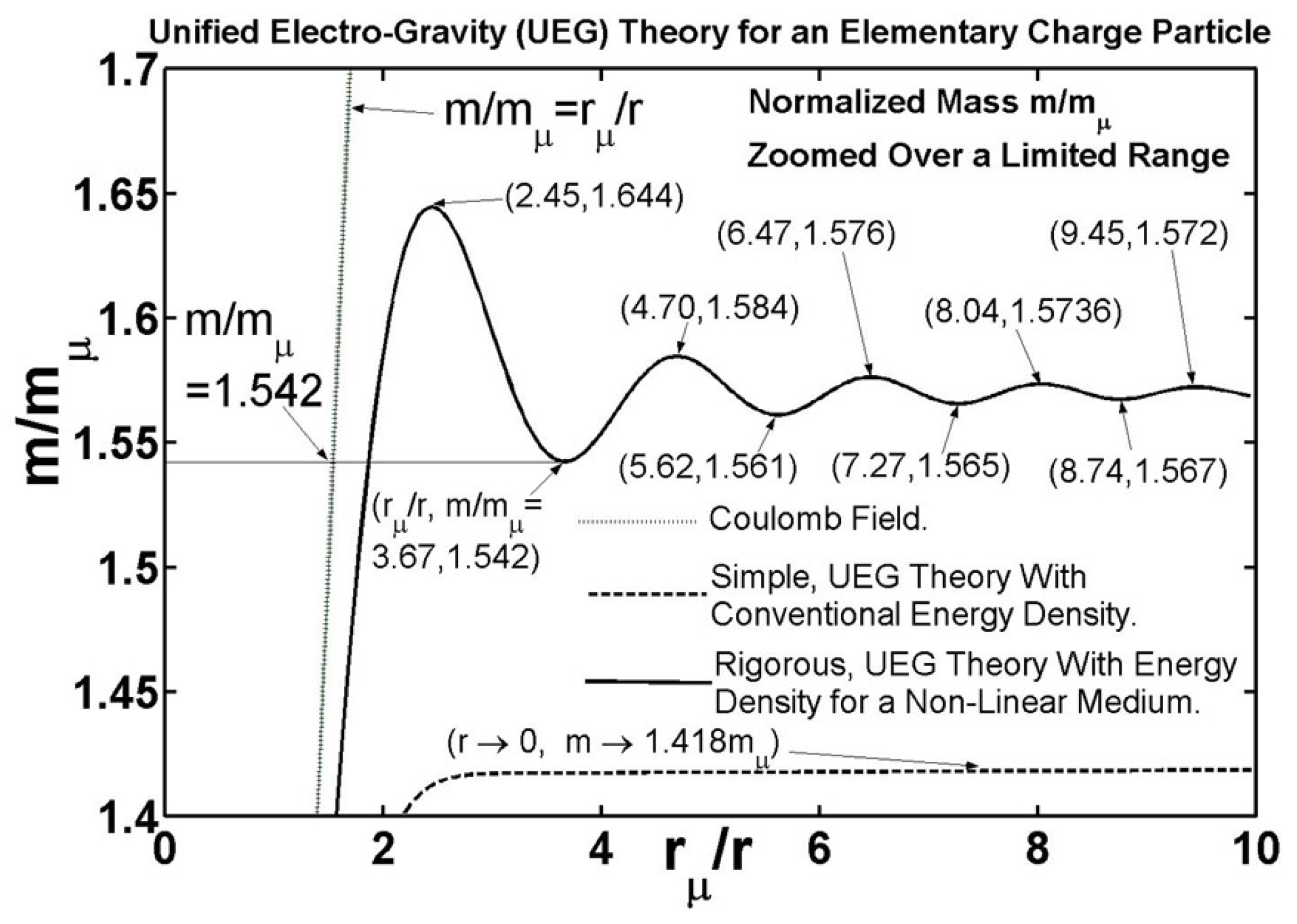
Figure 2 and Figure 3 (with different mass scales/resolutions) plot the normalized mass $m/m_{\mu }$ of (9) as a function of the normalized radius $r_{\mu }/r$, showing the oscillatory behavior of the mass function, as we anticipated earlier. Any of the minimum points of the mass function would correspond to a possible stable particle with the particular charge radius, as we also anticipated. The mass $m=m_0$ that would have resulted, if the inverse-relative permittivity function of (8) were used in the derivation of (9,4), based on a simplistic (incorrect) UEG model assuming a linear medium, is expressed in (10). This mass (10) normalized with respect to $m_{\mu }$ is also plotted in Figures 2,3 for reference, showing no stable radius. Also plotted in Figures 2,3 for reference is the normalized mass $(m/m_{\mu })=(r_{\mu }/r)$, based on a simple Coulomb’s field, which asymptotically approaches the normalized masses of (9) and (10) for $r\to \infty$, as should be expected. Clearly, the Coulomb mass does not allow any stable radius.

Figure 2.

Figure 2.

$$\begin{array}{cc}& m=m_0={\displaystyle \frac{W}{c^2}}={\displaystyle \frac{q^2}{8\pi c^2{ϵ}_0}}\underset{r}{\overset{\infty }{\int }}{\displaystyle \frac{{\underline{ϵ}}_r\left(r\right)}{r^2}}dr\\ & =m_{\mu }\sum _{k=0}^{\infty }{\displaystyle \frac{{(-1)}^k{t}^{(2k+\frac{2}{3})}}{2^{2k}k!(3k+1)}}.\end{array}$$

(10)

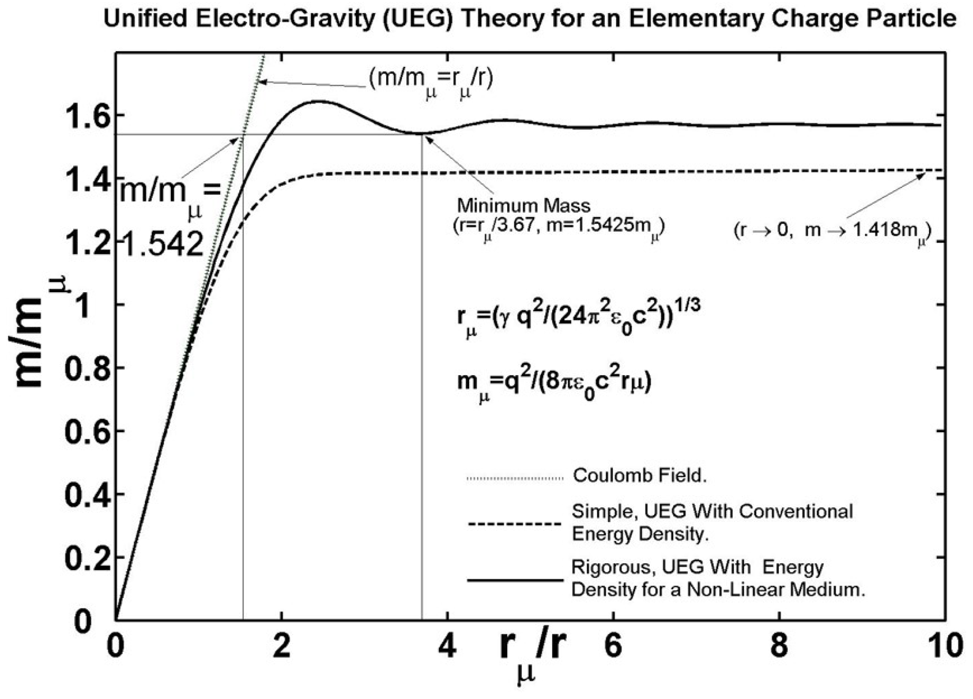
The smallest possible stable mass deduced from the oscillatory mass of (9) (Figures 2,3) is expected to be the mass of an electron (or a positron) without any spin. This is referred to as the static UEG mass $m_e^{\prime }$ of an electron. As deduced in (15), we will assume that the static UEG mass $m_e^{\prime }$ of an electron is about half of the total electron mass $m_e$, that includes additional mass/energy due to the electron’s spin. With this assumption of $m_e^{\prime }=m_e/2$ for the minimum stable mass in Figures 2,3, the value of the normalization constant $m_{\mu }$ can be calculated, from which the value of the UEG constant $\gamma$ is estimated.

$$\begin{array}{cc}& {\displaystyle \frac{m_e^{\prime }}{m_{\mu }}}={\displaystyle \frac{m_e}{2m_{\mu }}}=1.5425,\\ & m_{\mu }={\displaystyle \frac{m_e}{3.085}}=2.49\times {10}^{-30}{\gamma }^{-1/3},\\ & {\gamma }^{1/3}=3.085\times 2.49\times {10}^{-30}/m_e,\\ & \gamma =5.997\times {10}^2(m/s^2)/(J/m^3).\end{array}$$

(11)

As per the UEG theory of the electron, the constant $\gamma$ is declared to be a new natural constant, which is equal to a new gravitational acceleration in $m/s^2$ toward the center of gravity, produced due to one $J/m^3$ of energy density.

2.4. General Relationship Between the UEG Constant $\gamma$, the Particle Mass and Classical Radius

The above estimate of the value of the UEG constant $\gamma$ is associated with the actual value of the UEG static mass $m_e^{\prime }$ of the electron, and carries a specific dimensional unit of $(m/s^2)/(J/m^3)$. More fundamentally, a dimension-less relationship between the smallest stable UEG static mass $m_e^{\prime }$ of any elementary particle, the corresponding classical radius $r_e^{\prime }$, and the UEG constant $\gamma$ required to produce the mass $m_e^{\prime }$, can be derived based on the expressions for the reference mass $m_{\mu }$ (9) and reference radius $r_{\mu }$ (6) used in the above analysis.

$$\begin{array}{cc}& {\left({\displaystyle \frac{m_{\mu }}{m_e^{\prime }}}\right)}^3={\displaystyle \frac{3q^4}{{64\pi c}^4{ϵ}_0^2\gamma {m_e^{\prime }}^3}}={\displaystyle \frac{3{r_e^{\prime }}^2\pi }{\gamma m_e^{\prime }}},\\ & {\displaystyle \frac{\gamma m_e^{\prime }}{{r_e^{\prime }}^2}}=3\pi {\left({\displaystyle \frac{m_e^{\prime }}{m_{\mu }}}\right)}^3,m_e^{\prime }={\displaystyle \frac{q^2}{8\pi {ϵ}_0{r}_e^{\prime }{c}^2}}.\end{array}$$

(12)

The value of the ratio $m/m_{\mu }=1.5425$ from the Figures 2,3, for the smallest possible stable mass $m=m_e^{\prime }$. Using this value, the $\gamma$, $m_e^{\prime }$ and $r_e^{\prime }$ maybe related in term of a dimensionless constant.

$$\begin{array}{cc}& {\displaystyle \frac{\gamma m_e^{\prime }}{{r_e^{\prime }}^2}}=3\pi {\left({\displaystyle \frac{m_e^{\prime }}{m_{\mu }}}\right)}^3=34.590.\end{array}$$

(13)

If we simply assume the total mass $m_e$ of the elementary particle with spin to be twice the UEG mass $m_e^{\prime }$, and the classical radius $r_e$ associated with $m_e$ half of that ($=r_e^{\prime }$) with $m_e^{\prime }$, the $\gamma$, $m_e$ and $r_e$ may be related using a new dimensionless constant, which would be eight times the above constant.

$$\begin{array}{cc}& {\displaystyle \frac{\gamma m_e}{r_e^2}}=24\pi {\left({\displaystyle \frac{m_e^{\prime }}{m_{\mu }}}\right)}^3=8\times 34.590=276.720.\end{array}$$

(14)

Notice that the above constant is close to twice the inverse-fine structure constant $1/\alpha =137.036$ [22,23], and the earlier constant in (13) is one fourth of the $1/\alpha$, with less than one percent of difference. The small difference may be due to lack of generality or rigor of the basic UEG static theory for the particle, presented in this paper with assumption of a simple UEG function in (2), and without including the particle’s spin. The small difference may perhaps be related to the small difference between the actual value of the g-factor and its ideal value of 2 as discussed before. This may point to possible physical origin of the g-factor associated with the spin, governed by a more rigorous version of the new UEG theory.

Figure 3.

Figure 3.

Leaving aside any small difference due to lack of generality or rigor of the basic UEG model, the close relations of the above dimensionless constant (13 or 14) to the fine-structure constant is intriguing. First, the very existence of a dimensionless constant based on the UEG theory, and its intriguing close numerological relationship with the known fine-structure constant $\alpha$, may strongly suggest certain fundamental basis and significance of the new UEG theory. This is further supported by relating the UEG theory to the Casimir effect [15,16], where essentially the same close numerological relationship (13 or 14) to the fine-structure constant is also deduced. The close numerological relationship would strongly suggest a close direct, physical relationship between the UEG constant $\gamma$ associated with the dimensionless constant (13 or 14) from the UEG theory, and the particle’s quantum-theoretical spin angular momentum $\hslash /2$ (consequently, the Plank’s constant ℏ) associated with the fine-structure constant $\alpha$. The UEG theory of the static electron would now be extended in the following section, to model an electrodynamic problem of a physically spinning charge. This model would explore the anticipated direct physical relationship between the UEG theory and the quantum spin theory (and quantum theory in general), and consequently between the associated dimensionless constant (13 or 14) and the fine-structure constant $\alpha$, respectively.

3. Electron Spin Modeled as Orbiting of a Static UEG Electron, Around its Own Fields

Consider a static UEG electron, which is originally modeled as a stable charge body using the basic, static UEG theory of Section 2. Then, consider the static UEG electron to spin at radius $r_0$ at a speed $v_0$, close to the speed of light c, the central acceleration of which could be sustained by suitable UEG force(s). Clearly, the basic UEG theory of Section 2 which rigorously models the static UEG charge without spin, may no longer be rigorously valid for the spinning charge. A dynamic UEG theory for a moving charge would be required, that would include additional UEG forces due to energy density of the magnetic field, as well as UEGravito-magnetic effects due to the field momentum associated with the electromagnetic fields. The development of a such a complete dynamic theory, referred to as a unified electro-gravito-magnetic (UEGM) theory, is premature at this point, beyond the scope of the present work. However, in absence of such a full dynamic theory, we will model the spin behavior using a quasi-static UEG model, complemented by established results and insights from quantum electrodynamics.

A static UEG electron (modeled by a static UEG theory) may spin at a specific radial distance and velocity, that could be sustained by the UEG forces due to its own fields. The spinning of the static UEG electron maybe considered equivalent to orbiting of a complete electron structure (that already spins) around a central nucleus at a suitable orbital radius. Except, the complete-electron orbiting is sustained by the electric fields of an external body, the nucleus, whereas the spinning of the electron is sustained by the UEG forces due to the fields produced by the electron itself. The spinning electron may be treated similar to an orbiting electron with orbital quantum number equal to one, where the complete electron mass $m_e$ (already including the spin effects) for the orbiting electron is substituted by the static UEG mass $m_e^{\prime }$ of the “bare” (without the spin) electron. We know from quantum electrodynamics, that the magnetic moment ${\mu }_J$ due to an orbiting electron with orbital quantum number equal to one, is about the same as that due to a spinning electron, different by a factor $\underline{g}=g/2$ [25] close to unity. This means the velocity-radius products of the orbiting and the spinning electrons are also close to each other, different with the same above factor $\underline{g}$. In addition, we also know from quantum electrodynamics, that the angular momentum J of the orbiting and spinning states are ℏ and $\hslash /2$, respectively, different exactly by a factor of two. Based on the above information we already have, it can be deduced that the total mass $m_e$ (with spin) of the orbiting electron is $g(=2\underline{g})$ times, or about twice, the mass $m_e^{\prime }$ of a static UEG electron (without spin, modeled by a static UEG theory). Also can be deduced, that the angular momentum of the spinning electron is exactly equal to the above mass $m_e^{\prime }$ of the bare static UEG electron, multiplied by the velocity-radius product, $\left(v_0{r}_0\right)$ of the spinning electron.

$$\begin{array}{cc}& {\mu }_J={\displaystyle \frac{q}{2}}\times \left(vr\right),\\ & {\mu }_J\left(\mathrm{spin}\right)\simeq {\mu }_J\left(\mathrm{orbital}\right)={\displaystyle \frac{\hslash q}{2m_e}}={\displaystyle \frac{1}{\underline{g}}}{\mu }_J\left(\mathrm{spin}\right),\\ & {\left(vr\right)}_{\mathrm{spin}}\simeq {\left(vr\right)}_{\mathrm{orbital}}={\displaystyle \frac{\hslash }{m_e}}={\displaystyle \frac{1}{\underline{g}}}{\left(vr\right)}_{\mathrm{spin}},\\ & \underline{g}={\displaystyle \frac{g}{2}}=1.00115965218091,\\ & \\ & J=m\times \left(vr\right),J\left(\mathrm{spin}\right)={\displaystyle \frac{1}{2}}J\left(\mathrm{orbital}\right)={\displaystyle \frac{\hslash }{2}},\\ & m_e^{\prime }{\left(vr\right)}_{\mathrm{spin}}={\displaystyle \frac{1}{2}}{m}_e{\left(vr\right)}_{\mathrm{orbital}}={\displaystyle \frac{\hslash }{2}}\\ & \\ & m_e^{\prime }\simeq {\displaystyle \frac{1}{2}}{m}_e=\underline{g}{m}_e^{\prime },m_e=g{m}_e^{\prime },\\ & J\left(\mathrm{spin}\right)={\displaystyle \frac{\hslash }{2}}={\displaystyle \frac{J\left(\mathrm{orbital}\right)}{2}}={\displaystyle \frac{m_e}{2}}{\left(vr\right)}_{\mathrm{orbital}}\\ & =\left(\underline{g}{m}_e^{\prime }\right){\displaystyle \frac{1}{\underline{g}}}{\left(vr\right)}_{\mathrm{spin}}=m_e^{\prime }{\left(vr\right)}_{\mathrm{spin}}=m_e^{\prime }{v}_0{r}_0.\end{array}$$

(15)

As we deduced, the ratio between the spinning and the static electron masses is approximately equal to two. One might casually expect the ratio to be equal to the relativistic boost factor, which is dependent on the spin speed, as per special relativity. However, as mentioned before, we anticipate the spinning speed $v_0$ to be close to the speed of light c, in which case the relativistic boost factor would be much larger than the above ratio close to two. Accordingly, this might appear, at first, to be a contradiction to the casual expectation, but that may not be a valid observation. The mass transformation relation of special relativity is applicable only to a complete, stable massive particle in motion, but not for transformation of mass of the static UEG electron as it spins. This is because, the static UEG electron is an ideal state that is not dynamically stable in motion, and therefore does not constitute a complete, valid particle by itself to which special relativity can be independently applied. The static UEG electron is only a part of the internal formation of the complete electron structure, and the special relativity can only be applied to the complete structure. Further, the environment around a spinning electron, which is governed by the UEG theory involving non-linear deformation of the free-space structure around the electron, is significantly different from a simple free-space medium assumed in the special relativity. Accordingly, the principles of special relativity may not apply strictly in their conventional forms, in this spinning environment, particularly for transformation of mass.

The angular momentum relation of (15) may now be used to express the ratio of the spin radius $r_0$ and an equivalent radius $r_e^{\prime }$ of the static UEG electron, in terms of the fine structure constant $\alpha$ [22,26]. The ratio is approximately equal to $1/\alpha$, assuming that the spin velocity $v_0$ is close to the speed of light c.

$$\begin{array}{cc}& m_e^{\prime }{r}_0{v}_0={\displaystyle \frac{q^2{r}_0{v}_0}{8\pi {ϵ}_0{r}_e^{\prime }{c}^2}}={\displaystyle \frac{\hslash }{2}},m_e^{\prime }={\displaystyle \frac{q^2}{8\pi {ϵ}_0{r}_e^{\prime }{c}^2}},\\ & {\displaystyle \frac{r_0}{r_e^{\prime }}}={\displaystyle \frac{4\pi {ϵ}_0\hslash c}{q^2}}\left({\displaystyle \frac{c}{v_0}}\right)={\displaystyle \frac{1}{\alpha }}\left({\displaystyle \frac{c}{v_0}}\right)\simeq {\displaystyle \frac{1}{\alpha }},v_0\simeq c.\end{array}$$

(16)

4. UEG Acceleration Components that Support the Spinning Central Motion)

The fields and dynamics of a moving charged body with an expected speed close to the speed of light would need special modeling and interpretation. We would show in the following Section 6 that the UEG acceleration due to the energy density of the magnetic field of the spinning charge would cancel with the UEGravito-Magnetic acceleration produced by the momentum distribution associated with the equivalent UEG mass/energy distribution. Therefore, the central acceleration of the spinning charge would be sustained only by the remaining UEG acceleration due to energy density of the electric field. The central spinning motion of the electron, thus balanced by all the UEG and the UEG-Magnetic effects, may all be viewed as gravitational in nature in the fundamental sense. Accordingly, consistent with general relativity, a moving frame attached to the spinning orbit may be interpreted as an orbiting inertial frame (primed frame), moving along with the charge body, and the orbiting frame would be inertially equivalent to an external stationary frame (unprimed frame) far from the spinning center. We would estimate the electric field, electric energy density, and the associated UEG acceleration in the external stationary frame. This UEG-acceleration due to the electric energy density of the spinning electron, as seen in the external unprimed frame, would support the central acceleration of the spinning body. Space-time relations of special relativity may be used, for relativistic transformation between the external unprimed frame and the spinning primed frame.

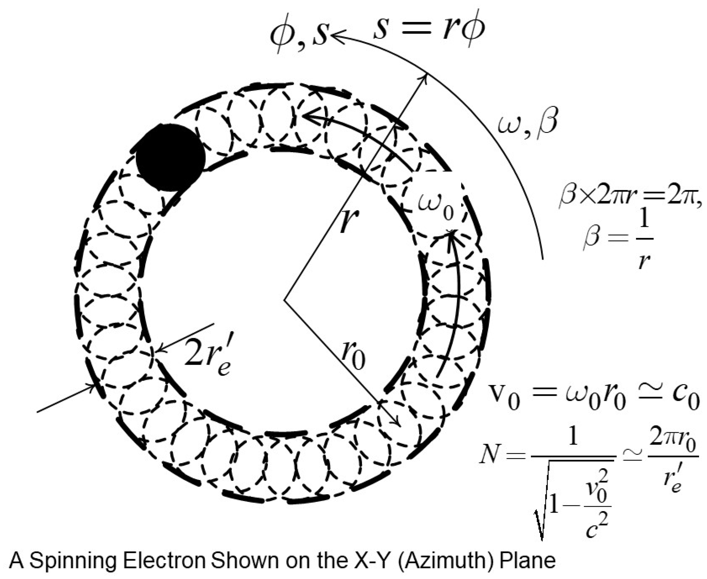
A length parameter, radius $r_e^{\prime }$ of the charge, along the orbital motion, as seen at a given instant in the orbiting primed frame, would be multiplied by the relativistic boost factor $(=N)$ as seen in the external unprimed frame. Accordingly, one may interpret that the electronic charge would “look stretched” along the orbit by the boost factor $\left(N\right)$. If $N=2\pi r_0/r_e^{\prime }$, the charge may appear wrapped around the spinning orbit, satisfying a suitable periodic physical condition. The periodic condition may be assumed to be a required “resonant” condition in a dynamic UEG theory, yet to be rigorously developed, in order to maintain a stable spin structure. Under this resonant condition, the stretched charge may be viewed in the form of N number of virtual unit cells, that are periodically arranged with proper overlap (assumed overlap factor 2) between neighboring units, over the entire circumference of the spin orbit (see Figure 4). Accordingly, the spinning charge may be viewed as a ring-charge, as well as a ring-current distribution. In fact, because the spinning orbit is actually in random orientations, with the spin-axis pointing randomly in all possible directions, the charge may be viewed to be wrapped around the entire surface of a sphere of radius equal to the spin radius $r_0$. Accordingly, the structure may be approximately modeled as a spinning surface-charge distribution, uniformly distributed over the sphere of radius $r_0$, with axis of the spinning randomly changing in time.

Figure 4.

Figure 4.

As per the above model, we would derive the average electric energy density at radial distance $r_0$, as seen by the external unprimed frame, by assuming a spherically symmetric electric field. The average electric energy density may first be expressed assuming that the uniform charge distribution on the sphere of radius $r_0$ is stationary with respect to the unprimed frame, having only radial electric field. When the charge spins, the radial electric field at a given point, which is directed orthogonal to the spinning velocity at the point, is expected to be increased by the relativistic boost factor N, as per special relativity. Consequently, the average electric energy density that we derived first, assuming the stationary charge distribution, may now be multiplied by the square of the boost factor, in order to find the average electric energy density of the spinning electron. This average electric energy density would be used to calculate the UEG acceleration to support the central acceleration of the spinning charge.

$$\begin{array}{cc}& \underline{E}={\displaystyle \frac{q}{4\pi {ϵ}_0{r}_0^2}}{\displaystyle \frac{1}{\sqrt{1-\frac{v_0^2}{c^2}}}}={\displaystyle \frac{qN}{4\pi {ϵ}_0{r}_0^2}},\\ & N=\sqrt{1-{\displaystyle \frac{v_0^2}{c^2}}}=a\times \left({\displaystyle \frac{2\pi r_0}{r_e^{\prime }}}\right)\simeq \left({\displaystyle \frac{2\pi r_0}{r_e^{\prime }}}\right),a\simeq 1.\end{array}$$

(17)

5. Planck’s and Fine Structure Constants Related to the UEG Constant Using the Spin Model

As discussed earlier, the central acceleration of the spin is to be sustained only by the UEG force due to the average electric energy density at the radius $r_0$. The UEG force due to magnetic energy density is assumed to be balanced by the UEGravito magnetic force, as shown in Section 6.

As per the charge model discussed above, the charge structure of Figure 4 maybe effectively interpreted in the form of overlapping (overlapping factor 2) square grids of $2r_e^{\prime }$ x $2r_e^{\prime }$ size each, wrapped in a ring configuration around the sphere of radius $r_0$. Further, because the axis of the ring structure of Figure 4 is randomly changing in time, the $2r_e^{\prime }$ x $2r_e^{\prime }$ sized grid structure would be effectively overlapping in two dimensions, wrapped over the surface of the sphere. Therefore, the UEG force at the center of the grid may be calculated by multiplying the average energy density on the spherical surface by a factor $(4/\pi )$. The factor is equal to the ratio of the area of a $r_e^{\prime }$ x $r_e^{\prime }$ (excluding overlap region) square grid to that of an enclosed circle of radius $r_e^{\prime }$. This geometric factor may be considered an empirical “filling factor,” necessary for proper estimation of the effective UEG force seen at the center of the spinning electron.

$$\begin{array}{cc}& {\underline{W}}_{\tau }={\displaystyle \frac{{ϵ}_0}{2}}{\underline{E}}^2={\displaystyle \frac{{ϵ}_0}{2}}{\left({\displaystyle \frac{q}{4\pi {ϵ}_0{r}_0^2}}\right)}^2{\left(N\right)}^2\simeq {\displaystyle \frac{{ϵ}_0}{2}}{\left({\displaystyle \frac{q}{4\pi {ϵ}_0{r}_0^2}}\right)}^2{\left({\displaystyle \frac{2\pi r_0}{r_e^{\prime }}}\right)}^2,\\ & E_g\simeq \gamma W_{\tau }\left({\displaystyle \frac{4{r^{\prime }}^2}{\pi {r^{\prime }}^2}}\right)\simeq \gamma {\displaystyle \frac{{ϵ}_0}{2}}{\left({\displaystyle \frac{q}{4\pi {ϵ}_0{r}_0^2}}\right)}^2{\left({\displaystyle \frac{2\pi r_0}{r_e^{\prime }}}\right)}^2\left({\displaystyle \frac{4}{\pi }}\right)={\displaystyle \frac{v_0^2}{r_0}}\simeq {\displaystyle \frac{c^2}{r_0}},\\ & {\displaystyle \frac{\gamma m_e^{\prime }}{{r_e^{\prime }}^2}}=\gamma {\displaystyle \frac{q^2}{8\pi {ϵ}_0{r_e^{\prime }}^3{c}^2}}\simeq {\displaystyle \frac{r_0}{4r_e^{\prime }}},\\ & {\displaystyle \frac{r_0}{r_e^{\prime }}}\simeq 4{\displaystyle \frac{\gamma m_e^{\prime }}{{r_e^{\prime }}^2}}=138.359\left(\mathrm{UEG}\mathrm{Theory}\right),\\ & {\displaystyle \frac{r_0}{r_e^{\prime }}}={\displaystyle \frac{1}{\alpha }}\left({\displaystyle \frac{c}{v_0}}\right)={\displaystyle \frac{1}{\alpha }}\left({\displaystyle \frac{1}{\sqrt{1-\frac{1}{N^2}}}}\right)\\ & \simeq {\displaystyle \frac{1}{\alpha }}={\displaystyle \frac{4\pi {ϵ}_0\hslash c}{q^2}}\simeq 137.036\left(\mathrm{QED}\right).\end{array}$$

(18)

The angular momentum associated with the above spinning would be equal to $\hslash /2$, as expected from quantum electrodynamics. The required ratio of the spin-radius $r_0$ and the charge-radius $r_e^{\prime }$, as derived in (16) from quantum electrodynamics, is approximately equal to the inverse of the fine structure constant $\alpha$ [26]. This ratio $r_0/r_e^{\prime }$ is shown above in (18) to approximately compare to that $r_0/r_e^{\prime }=4\gamma m_e^{\prime }/\left({r_e^{\prime }}^2\right)$ independently estimated from the UEG theory, based on the spinning model of Figure 4, using the UEG constant $\gamma$ derived in (14) from a static UEG model of an electron. The small fractional difference between the above two results for the ratio $r_0/r_e^{\prime }$ is calculated to be of the order of the fine structure constant. Conversely, if one would estimate the UEG constant $\gamma ={r_e^{\prime }}^2/\left(4\alpha m_e^{\prime }\right)$ from the above UEG theory and spin model, using the ratio $1/\alpha =r_0/r_e^{\prime }$ (16) from quantum electrodynamics, and known values of the electron mass $m_e^{\prime }=m_e/g$ from (15) and corresponding electron radius $r_e^{\prime }$ from (17), the value of $\gamma$ would be different from that in (14) derived from a static UEG electron model. The two different independent values of $\gamma$ would introduce a fractional ambiguity close to the fine structure constant, which we will address shortly in the following Section 5.1.

$$\begin{array}{cc}& \gamma \left(\mathrm{UEG}\right)=138.359\times {\displaystyle \frac{{r_e^{\prime }}^2}{4m_e^{\prime }}}\\ & =138.359\times {\displaystyle \frac{r_e^2{g}^3}{4m_e}}\simeq 6.017\times {10}^2\left(\mathrm{m}{\mathrm{s}}^{-2}\right)/\left(\mathrm{J}{\mathrm{m}}^{-3}\right),\\ & \gamma \left(\mathrm{QED}\right)=137.036\times {\displaystyle \frac{{r_e^{\prime }}^2}{4m_e^{\prime }}}\\ & =137.036\times {\displaystyle \frac{r_e^2{g}^3}{4m_e}}\simeq 5.96\times {10}^2\left(\mathrm{m}{\mathrm{s}}^{-2}\right)/\left(\mathrm{J}{\mathrm{m}}^{-3}\right),\\ & \gamma \left(\mathrm{UEG}\right)-\gamma \left(\mathrm{QED}\right)\\ & \simeq \gamma \left(\mathrm{QED}\right)\times 1.32\alpha \sim \gamma \left(\mathrm{QED}\right)\times \alpha .\end{array}$$

(19)

Leaving aside the small fractional ambiguity, discussed above, the close results from the UEG theory and quantum electrodynamics point to a definite fundamental connection between the two theories, relating the UEG constant $\gamma$ to the fine structure constant $\alpha$. This is a significant development, also providing a direct physical relation between the UEG constant $\gamma$ and the Plancks constant ℏ, via the fine structure constant $\alpha$ to which both the $\gamma$ and ℏ are related to, founded on the dynamic modeling of the spin, sustained by the UEG forces. In other words, the Planck’s constant ℏ, with its origin in quantum mechanics, may no longer be considered a fully independent natural constant, but is rather unified together with the UEG constant $\gamma$. Accordingly, the UEG theory, which already unifies the electric and gravitational principles, is now positioned to be fully unified with quantum mechanics as well.

5.1. Closer Relationship Between the UEG and Quantum Electrodynamics

It may be noted that the UEG theory from which the constant $\gamma$ was estimated in (18) is only a basic theory, where the UEG acceleration is assumed to be proportional to the energy density, with $\gamma$ as the constant of the proportionality. A rigorous UEG theory would include higher-order acceleration proportional to higher powers of the energy density, which is expected to reduce the value of the stable mass $m_e^{\prime }$, as compared to that from the basic theory in Section 2 with a given $\gamma$ without the higher-order terms. Conversely, in order to have the same final stable mass $m_e^{\prime }$, one may need to start with a basic UEG theory producing a higher stable mass, or equivalently with a lower $\gamma$, before introducing higher-order UEG terms. In other words, the actual value of $\gamma$ in the dominant acceleration in a rigorous UEG theory, which is the the constant of proportionality between the UEG acceleration and the energy density, in the low energy-density range, is expected to be lower than than the value of $\gamma$ in Section 2 obtained from a basic UEG theory without any higher-order effects. This is under the condition that the rigorous and the basic UEG theories produce the same static electron mass $m_e^{\prime }$. The lower value of $\gamma$ in the rigorous theory would be associated with a reduction of the effective radius $r_e^{\prime }$, in proportion to the cube-root of $\gamma$ as per (14).

Based on the above discussion, we may recognize that in principle there are three theoretical values for the constant $\gamma$. $\left(I\right)$ The value of $\gamma$ obtained from a basic UEG theory of Section 2, that produces a stable electron mass equal to $m_e^{\prime }=m_e/g$. $\left(II\right)$ The actual value of the $\gamma$, which is the constant of proportionality between the UEG acceleration and the energy density, valid when the energy density is sufficiently small. This would be the dominant term, or the first order approximation, in a fully rigorous UEG theory. And, $\left(III\right)$ the value of the $\gamma ={r_e^{\prime }}^2/\left(4\alpha m_e^{\prime }\right)$ that is indirectly estimated from an ideal spin model of the electron, as derived in Section 5, which expects the known fine structure constant from quantum electrodynamics to be related to the $\gamma$, and the known values of the electron mass $m_e^{\prime }$ and the electron radius $r_e^{\prime }$. A higher-order UEG theory for a bare, static electron, combined with a rigorous, dynamic UEG model for a spinning electron would be needed to explain any differences or specific relationship between the three parameters, which is beyond any scope of the present work. The parameters $\left(I\right)$ and $\left(III\right)$ are shown in (19) to be close to each other with a fractional difference of the order of the fine structure constant, and we may suspect similar closeness of the parameter $\left(II\right)$ to the other two values. Additional insight may assist in more accurate evaluation for the parameter $\left(II\right)$, which is the actual constant of proportionality between UEG acceleration and energy density, in an environment with low energy density.

The effective radius used in an ideal spin model of Section 3, Figure 4, is assumed to be the classical radius $r_e^{\prime }$ of the bare electron, which determines the required relativistic boost factor to be ideally equal to $N=2\pi r_0/r_e^{\prime }$. The actual value of the boost factor is slightly larger than this ideal value, represented by the factor a, the value of which can be estimated as shown in (21), from the known values of the fine structure constant $\alpha$ and electron g-factor. This increase is equivalent to having an effective radius $r_e^{\prime }$ to be smaller than the ideal value by the same factor a. It may be reasonable to estimate that the actual increased value of the boost factor $N=2\pi r_{0}a/r_e^{\prime }$, and the corresponding reduced effective radius $r_e^{\prime }/a$, is associated with the average between the two values of $\gamma$$\left(I\right)$ and $\left(II\right)$, that is the average between the values needed in a basic UEG model and in a rigorous UEG model to produce the same stable mass $m_e^{\prime }$. Whereas, the ideal value of the boost factor $N=2\pi r_0/r_e^{\prime }$, and the corresponding effective radius $r_e^{\prime }$, is associated with the first value of $\gamma$$\left(I\right)$, that is the value needed in a basic UEG model to produce the stable mass $m_e^{\prime }$. As per the earlier discussion on the effect of the higher-order UEG theory, the reduction in the effective radius would mean that the average of the two values of $\gamma$$\left(I\right)$ and $\left(II\right)$ would be lower than the first value of $\gamma$$\left(I\right)$, by a factor equal to $a^3\simeq 1.0045\simeq 1+0.62\alpha$ (see (21)). This would place the estimate for the actual value of $\gamma$$\left(II\right)$, fractionally about $(1+1.24\alpha )$ lower than the estimate of $\gamma$$\left(I\right)$ from the basic UEG theory. This estimate for the actual value of the $\gamma$$\left(II\right)$ is fairly close to the estimate $\left(III\right)$ from quantum electrodynamics, which we know from (19) to be fractionally about $(1+1.32\alpha )$ lower than the estimate $\left(I\right)$. In other words, the estimates of $\gamma$$\left(II\right)$ and $\left(III\right)$ would be essentially equal to each other with a fractional difference of less than $0.1\alpha$, or within $0.1\%$.

$$\begin{array}{cc}& \gamma \left(\mathrm{actual}\right)\simeq {\displaystyle \frac{\gamma \left(\mathrm{Basic}\mathrm{UEG}\right)}{(1+2a^3)}}\\ & ={\displaystyle \frac{\gamma \left(\mathrm{Basic}\mathrm{UEG}\right)}{(1+1.24\alpha )}}=5.963\times {10}^2\left(\mathrm{m}{\mathrm{s}}^{-2}\right)/\left(\mathrm{J}{\mathrm{m}}^{-3}\right),\\ & \gamma \left(\mathrm{QED}\right)\simeq {\displaystyle \frac{\gamma \left(\mathrm{Basic}\mathrm{UEG}\right)}{(1+1.32\alpha )}}=5.96\times {10}^2\left(\mathrm{m}{\mathrm{s}}^{-2}\right)/\left(\mathrm{J}{\mathrm{m}}^{-3}\right),\\ & \gamma \left(\mathrm{actual}\right)\simeq \gamma \left(\mathrm{QED}\right),{\displaystyle \frac{\gamma \left(\mathrm{actual}\right)}{\gamma \left(\mathrm{QED}\right)}}<1.001.\end{array}$$

(20)

The parameter a, used in the above discussion and deduction, is expressed as follows, using (16) for the ratio $r_0/r_e^{\prime }$, and (29) to relate the boost factor N to the factor $\underline{g}$. The value of a may be calculated using known measured values of the fine structure constant $\alpha$ and the electron g-factor $g=2\underline{g}$ .

$$\begin{array}{cc}& {\displaystyle \frac{r_0}{r_e^{\prime }}}={\displaystyle \frac{4\pi {ϵ}_0\hslash c}{q^2}}({\displaystyle \frac{c}{v_0}})={\displaystyle \frac{1}{\alpha }}({\displaystyle \frac{c}{v_0}})={\displaystyle \frac{1}{\alpha }}({\displaystyle \frac{1}{\sqrt{1-\frac{1}{N^2}}}}),\\ & N=a\times ({\displaystyle \frac{2\pi r_0}{r_e^{\prime }}})={\displaystyle \frac{2\pi a}{\alpha }}({\displaystyle \frac{1}{\sqrt{1-\frac{1}{N^2}}}}),\\ & {\displaystyle \frac{1}{a}}={\displaystyle \frac{2\pi /\alpha }{N\sqrt{1-\frac{1}{N^2}}}}={\displaystyle \frac{(2\pi /\alpha )(\underline{g}-1)}{\sqrt{1-{(\underline{g}-1)}^2}}}\\ & =(2\pi /\alpha )\times 0.0011596529=1-0.0015126724.\end{array}$$

(21)

Based on the close estimated values $\left(II\right)$ and $\left(III\right)$ of $\gamma$, as discussed above, it may be suggested that the two values $\left(II\right)$ and $\left(III\right)$, namely, the value of $\gamma$ from a rigorous UEG model of electron, and the value $\gamma ={r_e^{\prime }}^2/\left(4\alpha m_e^{\prime }\right)$ derived from quantum electrodynamics, could be, after all, equal to each other, or close to each other with relatively higher precision. This proposition may be supported by further insights and more accurate modeling of the central acceleration of the spinning electron.

The above modeling in (18) of the spinning electron using the UEG theory was established in an approximate form, in the absence of a rigorous dynamic UEG theory, as an initial estimate in order to illustrate fundamental relations between the UEG and the fine structure constants. Conversely, when a rigorous dynamic UEG theory would be established and it validates the basic principles of the modeling (18), the fine structure and the Planck’s constants could in principle be derived and predicted exactly from the UEG theory. For now, we may evaluate the fine structure constant $\alpha$, which is the inverse of ratio of the spin radius and the electron radius, more accurately from the modeling of (18), guided by the following insight.

We know from (21) that the boost factor N is slightly larger than the ratio $(2\pi r_0/r_e^{\prime })$ obtained from the angular momentum in (16), by the factor a. This is equivalent to having increased overlap between the neighboring particles in the ring model of Section 3, Figure 4. The average energy density in (18) maybe properly redistributed over the surface of the spin sphere, weighted in proportion to the actual energy/mass distribution. Accordingly, the redistributed energy density at the particle center would be inversely proportional to the square of the overlap factor a, considering overlap of the spinning particle in two dimensions over the surface of the spin sphere. More is the overlap, which is on the outer edges of the particle, more energy density needs to be redistributed away from the center, leaving less energy density at the particle center. As a proposed hypothesis, this redistributed energy density, evaluated at the center of the particle, would be multiplied with the UEG constant $\gamma$, in order to obtain the UEG acceleration that supports the central acceleration. Accordingly, the UEG acceleration would be reduced by a factor $a^2$. This may be introduced as an multiplying factor $1/a^2$, in addition to the ideal redistribution factor $4/\pi$ that we already have in our model of (18).

$$\begin{array}{cc}& {\underline{W}}_{\tau }={\displaystyle \frac{{ϵ}_0}{2}}{\underline{E}}^2={\displaystyle \frac{{ϵ}_0}{2}}{\left({\displaystyle \frac{q}{4\pi {ϵ}_0{r}_0^2}}\right)}^2{\left(N\right)}^2={\displaystyle \frac{{ϵ}_0}{2}}{\left({\displaystyle \frac{q}{4\pi {ϵ}_0{r}_0^2}}\right)}^2{\left({\displaystyle \frac{2\pi r_0}{r_e^{\prime }}}\right)}^2{\left(a\right)}^2,\\ & E_g=\gamma {\underline{W}}_{\tau }\left({\displaystyle \frac{4{r_e^{\prime }}^2}{\pi {r_e^{\prime }}^2}}\right){\left({\displaystyle \frac{1}{a}}\right)}^2=\gamma {\displaystyle \frac{{ϵ}_0}{2}}{\left({\displaystyle \frac{q}{4\pi {ϵ}_0{r}_0^2}}\right)}^2{\left({\displaystyle \frac{2\pi r_0}{r_e^{\prime }}}\right)}^2\left({\displaystyle \frac{4}{\pi }}\right)={\displaystyle \frac{v_0^2}{r_0}},\\ & {\displaystyle \frac{\gamma m_e^{\prime }}{{r_e^{\prime }}^2}}=\gamma {\displaystyle \frac{q^2}{8\pi {ϵ}_0{r_e^{\prime }}^3{c}^2}}=\left({\displaystyle \frac{r_0}{4r_e^{\prime }}}\right){\left({\displaystyle \frac{v_0}{c}}\right)}^2\\ & =\left({\displaystyle \frac{r_0}{4r_e^{\prime }}}\right)(1-{\displaystyle \frac{1}{N^2}})=\left({\displaystyle \frac{r_0}{4r_e^{\prime }}}\right)(1-{(1-\underline{g})}^2).\end{array}$$

(22)

The expression for the ratio of the spin and classical static electron radii, derived from spin angular momentum relation (16), may now be used for a closer relationship between the rigorous UEG constant $\gamma$ to the fine structure constant $\alpha$.

$$\begin{array}{cc}& {\displaystyle \frac{r_0}{r_e^{\prime }}}={\displaystyle \frac{4\pi {ϵ}_0\hslash c}{q^2}}({\displaystyle \frac{c}{v_0}})={\displaystyle \frac{1}{\alpha }}({\displaystyle \frac{c}{v_0}})={\displaystyle \frac{1}{\alpha }}({\displaystyle \frac{1}{\sqrt{1-\frac{1}{N^2}}}})={\displaystyle \frac{1}{\alpha }}({\displaystyle \frac{1}{\sqrt{1-{(1-\underline{g})}^2}}}),\\ & {\displaystyle \frac{4\gamma m_e^{\prime }}{{r_e^{\prime }}^2}}=({\displaystyle \frac{r_0}{r_e^{\prime }}})(1-(1-{\underline{g}}^2))={\displaystyle \frac{1}{\alpha }}\sqrt{1-(1-{\underline{g}}^2)}={\displaystyle \frac{1}{\alpha }}\sqrt{1-{\displaystyle \frac{1}{N^2}}},\\ & ({\displaystyle \frac{4\gamma m_e^{\prime }}{{r_e^{\prime }}^2}})({\displaystyle \frac{r_0}{r_e^{\prime }}})={({\displaystyle \frac{1}{\alpha }})}^2.\end{array}$$

(23)

The dimensionless constant $4\gamma m_e^{\prime }/{r_e^{\prime }}^2$, where $\gamma$ is the rigorous UEG constant, and the other dimensional constant $1/\alpha$, which is the inverse of fine structure constant, are now shown in (23) to be close to each other with fractional difference of approximately $1/(2N^2)$. This fractional difference is of the order of the square of $\alpha /(2\pi )$, which would amount to having the above two dimensionless constants essentially equal to each other, with their ratio different from unity only in the sixth or higher decimal places. This is a significant development, which, in addition to reinforcing unmistakable unified connection between the UEG theory and quantum electrodynamics, opens valuable insights for any future development of a fully rigorous UEG theory. The effective $\gamma$ for a rigorous UEG theory is now very accurately estimated from a basic UEG theory and available information from quantum electrodynamics. Additional details for a rigorous UEG theory could also be extracted from the g-factor, the measured value of which is available with very high precision. This would be possible through the parameter a in (21), which is the change of the effective radius of the particle as compared to its ideal classical value $r_e^{\prime }$, carrying information that would constrain any variation of a general UEG function $\gamma (W_{\tau })$ in a rigorous UEG theory. This is in addition to the effective $\gamma$ deduced above, which would be the first-order constant coefficient of the general UEG function, which is only an approximation of the general UEG function for low energy density $W_{\tau }$.

6. The UEG Acceleration Due to the Magnetic Field, and the UEGM (UEGravito-Magnetic) Acceleration Due to the Field Momentum

We will find the expression of the velocity due to spinning at a given radius r. This may be derived from the electromagnetic field momentum, using the Coulomb electric field due to the electron charge and the magnetic field produced due to spin magnetic moment ${\mu }_S$. The velocity may also be estimated from a quantum-mechanical model where the spinning of the static mass $m_e^{\prime }$ is treated similar to the orbital motion of the total electron mass $m_e$. The two velocity expressions from the electromagnetic and the quantum models are similar except the $sin\theta$ factors.

$$\begin{array}{cc}& {\overline{\mu }}_S={\displaystyle \frac{\hslash q}{2m_e}}\widehat{z},\overline{H}=\widehat{\theta }{\displaystyle \frac{{\mu }_S}{4\pi r^3}}sin\theta +\widehat{r}{\displaystyle \frac{{\mu }_S}{2\pi r^3}}cos\theta ,\\ & \overline{E}=\widehat{r}{\displaystyle \frac{q}{4\pi \epsilon r^2}},\overline{v}(EM)={\displaystyle \frac{\overline{E}\times \overline{H}}{(\frac{\epsilon }{2}{E}^2)}}=\widehat{\varphi }{\displaystyle \frac{2{\mu }_{S}sin\theta }{qr}}=\widehat{\varphi }{\displaystyle \frac{\hslash sin\theta }{m_{e}r}},\\ & \overline{S}=m_e^{\prime }{\overline{r}}_0\times {\overline{v}}_0={\displaystyle \frac{1}{2}}{m}_e\overline{r}\times \overline{v}\\ & =\widehat{z}{\displaystyle \frac{1}{2}}{m}_e{v}_{\varphi }rsin\theta =\widehat{z}{\displaystyle \frac{\hslash }{2}},\overline{v}(QM)=\widehat{\varphi }{\displaystyle \frac{\hslash }{m_{e}rsin\theta }}.\end{array}$$

(24)

The energy density in the magnetic field would produce an UEG acceleration $E_{gum}$, which may be expressed by multiplying the average energy density in the magnetic field with the UEG constant $\gamma$.

$$\begin{array}{cc}& {\overline{E}}_{gum}=-\widehat{r}<\gamma ({\displaystyle \frac{\mu }{2}}{H}^2)>=-\widehat{r}{\displaystyle \frac{\gamma \mu {\mu }_S^2}{32{\pi }^2{r}^6}}<({sin}^2\theta +4{cos}^2\theta )>\\ & =-\widehat{r}{\displaystyle \frac{\gamma \mu {\mu }_S^2}{32{\pi }^2{r}^6}}{\displaystyle \frac{\underset{0}{\overset{\pi }{\int }}({sin}^2\theta +4{cos}^2\theta )sin\theta d\theta }{\underset{0}{\overset{\pi }{\int }}sin\theta d\theta }}\\ & =-\widehat{r}{\displaystyle \frac{\gamma \mu {\mu }_S^2}{16{\pi }^2{r}^6}}=-\widehat{r}{\displaystyle \frac{\gamma \mu q^2{\hslash }^2}{64{\pi }^2{m}_e^2{r}^6}}.\end{array}$$

(25)

Unlike a static electron without any spin, which produces a UEG force field and is associated with a gravitational mass distribution (mass-density) as per Gauss’ law, a spinning electron would in addition be associated with an effective UEG momentum distribution (momentum-density) that may be expressed by multiplying the UEG mass density and the velocity derived above. This momentum-density due to the moving UEG mass-density is expected to produce a gravito-magnetic field, in a very similar way as an electric current distribution due to a moving electric charge distribution produces a magnetic field as per the Ampere’s law of the electromagnetic theory. Accordingly, the gravito-magnetic field may also be derived from the UEG momentum density using an equivalent version of the Ampere’s law.

The acceleration due to the gravito-magnetic field may be expressed as the cross-product of gravito-magnetic field and the velocity. Note that there are two velocity terms in the above derivation: $(I)$ the velocity used in derivation of the gravito-magnetic field to begin with, and then $(II)$ the velocity that multiplies with the gravito-magnetic field to find the gravito-magnetic acceleration. As a reasonable approach to estimate the average gravito-magnetic acceleration, we choose the two velocity terms to be expressed differently as in (24) - the former derived quantum-mechanically $(\overline{v}(QM))$ and the later electromagnetically $(\overline{v}(EM))$. Also note that we treat the gravito-magnetic acceleration ${\overline{E}}_{gm}$ in (26) just like an equivalent acceleration in an electromagnetic modeling, without any adjustment factor. This is unlike conventional gravito-magnetic modeling [27] where an additional factor of $1/4$ might be needed. This is because, in conventional gravito-magnetic modeling [27] the mass, which is the source of gravitation, relativistically varies with velocity. Whereas, the average mass density ${\rho }_{vu}$ in the present modeling, associated with the azimuthal ($\widehat{\varphi }$-directed) is assumed to be independent of the velocity $\overline{v}$, just like the electric charge density, which is the source of an electromagnetic field, would be in an equivalent electromagnetic modeling.

$$\begin{array}{cc}& {\overline{E}}_{gue}=-\widehat{r}\gamma ({\displaystyle \frac{\epsilon }{2}}{E}^2)=-\widehat{r}{\displaystyle \frac{\gamma q^2}{32{\pi }^2\epsilon r^4}},\\ & {\rho }_{vu}=-\epsilon \overline{\nabla }·{\overline{E}}_{gue}=-{\displaystyle \frac{\gamma q^2}{16{\pi }^2{r}^5}},\\ & \overline{\nabla }\times {\overline{H}}_{gu}={\overline{J}}_{gu}={\rho }_{vu}\overline{v}(QM),{\overline{H}}_{gu}=\widehat{\theta }{H}_{gu\theta },\overline{\nabla }·{\overline{H}}_{gu}=0,\\ & {\displaystyle \frac{1}{r}}{\displaystyle \frac{\partial (r{H}_{gu\theta })}{\partial r}}={\rho }_{vu}{v}_{\varphi }(QM)=-{\displaystyle \frac{\gamma q^2\hslash }{16{\pi }^2{m}_e{r}^{6}sin\theta }},\\ & H_{gu\theta }={\displaystyle \frac{\gamma q^2\hslash }{64{\pi }^2{m}_e{r}^{5}sin\theta }},\\ & {\overline{E}}_{gm}=-\mu <\overline{v}\times {\overline{H}}_{gu}>=-\mu \overline{v}(EM)\times {\overline{H}}_{gu}\\ & =\widehat{r}\mu v_{\varphi }(EM)H_{gu\theta }=\widehat{r}\mu ({\displaystyle \frac{\hslash sin\theta }{m_{e}r}})({\displaystyle \frac{\gamma q^2\hslash }{64{\pi }^2{m}_e{r}^{5}sin\theta }})\\ & =\widehat{r}{\displaystyle \frac{\gamma \mu q^2{\hslash }^2}{64{\pi }^2{m}_e^2{r}^6}}.\end{array}$$

(26)

It is shown that the gravito-magnetic acceleration (26) due to UEG momentum density is negative of the UEG acceleration (25) due to the energy density in the magnetic field. Therefore, the total UEG force is simply the UEG force due to the energy density in the electric field, independent of the magnetic field generated due to the spin.

$$\begin{array}{cc}& {\overline{E}}_{gm}+{\overline{E}}_{gum}=0,\\ & {\overline{E}}_g={\overline{E}}_{gue}+{\overline{E}}_{gm}+{\overline{E}}_{gum}\\ & ={\overline{E}}_{gue}=-\widehat{r}\gamma ({\displaystyle \frac{\epsilon }{2}}{E}^2)=-\widehat{r}{\displaystyle \frac{\gamma q^2}{32{\pi }^2\epsilon r^4}}.\end{array}$$

(27)

The theory developed in this section is an important recognition of the existence and significance of the gravito-magnetic effect surrounding the electron, produced as per the new UEG theory. The gravito-magnetic effect constitutes a critical physical mechanism of the complete internal structure of the electron.

7. Quantum Mechanical Wave is a Ripple in the “Non-Linear” Free-Space Medium, With the Quantum Frequency Close to the Spin Frequency

The quantum mechanical (QM) wave of frequency $\omega$ may be viewed as a ripple in the free space produced due to the spinning of the electron, as a result of the strong UEG force. The non-linear permittivity function of the free-space in the UEG (static) theory would transform into the QM wave function of the “free-space” as a result of the spinning. It was discussed in Section 4, Section 6, that the strong UEG field around the spinning charge would produce an equivalent rotating inertial frame, dragged along with the moving charge due to the UEGravito-Magnetic (UEGM) effect. The frequency $\omega$ of the QM wave maybe intuitively “seen” as a difference-frequency $\omega -{\omega }_0$ relative to the rotating frame spinning with the frequency ${\omega }_0$. The difference frequency $\omega -{\omega }_0$, and the actual QM frequency $\omega$ may be related with each other by the relativistic boost factor N between the rotating frame (primed frame) and a stationary frame (unprimed frame) far from the spin center. Accordingly, the QM frequency $\omega$ may be shown to be slightly larger than the spin frequency ${\omega }_0$, with a small difference of $\omega /N$. The intuitive relationships may also be established using space-time transformation between the primed and unprimed frames, and enforcing a periodic symmetry condition ($\beta$ x $(2\pi r_0)$ =$2\pi$) around the circumference $2\pi r_0$ of the rotating frame.

This is a significant development, which provides a direct physical process that represents the QM wave, in the form of ripples produced due to spinning in a a non-linear free-space medium. This may be established by directly relating the QM wave frequency $\omega$ to the physical spinning frequency ${\omega }_0$ of the charge.

$$\begin{array}{cc}& e^{j\omega t}{e}^{-j\beta s}=e^{j{\omega }^{\prime }{t}^{\prime }}{e}^{-j{\beta }^{\prime }{s}^{\prime }},t={\displaystyle \frac{t^{\prime }+s^{\prime }{v}_0/c^2}{\sqrt{1-\frac{v_0^2}{c^2}}}},s={\displaystyle \frac{s^{\prime }+t^{\prime }{v}_0}{\sqrt{1-\frac{v_0^2}{c^2}}}},\\ & {\omega }^{\prime }={\displaystyle \frac{\omega -\beta v_0}{\sqrt{1-\frac{v_0^2}{c^2}}}},{\beta }^{\prime }={\displaystyle \frac{\beta -\omega v_0/c^2}{\sqrt{1-\frac{v_0^2}{c^2}}}},\\ & {\omega }^{\prime }=\omega ={\displaystyle \frac{\omega -v_0/r_0}{\sqrt{1-\frac{v_0^2}{c^2}}}}={\displaystyle \frac{\omega -{\omega }_0}{\sqrt{1-\frac{v_0^2}{c^2}}}};\\ & \beta \times (2\pi r_0)=2\pi ,\beta ={\displaystyle \frac{1}{r_0}}.\end{array}$$

(28)

For a general interpretation of the above concept of the quantum/UEG wave, first consider a “stationary” spinning charged body with a total mass m (including spin and static UEG mass) and linear momentum $p=0$, with no linear motion of the center of spinning. The region surrounding the charge will be associated with a space-time dependent permittivity function ${ϵ}_r(r,t)$ expressed in the harmonic form (28), which would represent the quantum/UEG wave function of the stationary particle. The wave will be seen by a stationary observer to be oscillating as $e^{j\omega t}$ with frequency $\omega$, but having no spatial dependence with wave number $\beta =1/r=0$, in the region far from the center $(r=\infty )$. We may assume that the wave amplitude in the far region is uniform in space, independent of the spatial variation of the UEG field. This wave function would be consistent with quantum mechanics, with the expected energy-wave frequency relationship $w=m{c}^2=\hslash \omega$, and momentum-wave number relationship $p=mv=\hslash \beta =0$.

Now, the above quantum-mechanical relationships for the “stationary” spinning charge may be extended as well when the charged body undergoes a linear motion of the center of spinning, with velocity v in a given direction s. Applying space-time transformation of special relativity, the above wave function $e^{j\omega t}$ of the stationary charge in the far region, dependent only on time, maybe shown to transform into a wave $e^{j\omega (t-sv/c^2)\eta }$ $=e^{j{\omega }^{\prime }t}{e}^{-j{\beta }^{\prime }s}$, with both space and time variation, as seen by a stationary observer. The new frequency ${\omega }^{\prime }=\eta \omega$$=\eta m{c}^2/\hslash$$=m^{\prime }{c}^2/\hslash$, and the new wave number ${\beta }^{\prime }={\omega }^{\prime }v/c^2$$=m^{\prime }v/\hslash$$=p^{\prime }/\hslash$, are related to the new mass $m^{\prime }=\eta m$ and momentum $p^{\prime }=m^{\prime }v$, where $\eta ={(1-v^2/c^2)}^{-0.5}$ is the relativistic boost factor associated with the velocity v. The basic quantum mechanical energy/momentum and frequency/wave number relationships, $W^{\prime }=m^{\prime }{c}^2={\omega }^{\prime }\hslash$ and $p^{\prime }=m^{\prime }v={\beta }^{\prime }\hslash$, are clearly established between the wave parameters in the region far from the center of the moving charge, and the mass $m^{\prime }$ and linear momentum $p^{\prime }$ of the physical charged body moving at the center of wave.

Clearly, the above quantum-mechanical relationships for the quantum/UEG wave would not be valid in the region closer to the central charge. A full dynamic UEG theory may be needed to rigorously model the wave function in the central region, particularly in the immediate vicinity of the charge with strong energy density.

7.1. Electron g-Factor Related to Relativistic Boost factor, and to the Spin and Quantum Wave Frequencies

Based on the above quantum-mechanical interpretation, the frequency $\omega$ in (28) may be related to the total electron mass $m_e$. On the other hand, the spin frequency ${\omega }_0$ is related to the static electron mass $m_e^{\prime }$ through the spin angular momentum $\hslash /2$. Accordingly, given that the two frequencies $\omega$ and ${\omega }_0$ are related to each other in (28) by the boost factor N, the total and the static masses would also be related to each other by the boost factor. Consequently, the electron g-factor, which is the ratio of the total and the static masses, would be directly related to the boost factor.

$$\begin{array}{cc}& {\displaystyle \frac{1}{\sqrt{1-\frac{v_0^2}{c^2}}}}=N,{\displaystyle \frac{\omega -{\omega }_0}{\sqrt{1-\frac{v_0^2}{c^2}}}}=N(\omega -{\omega }_0)=\omega ,\\ & \omega (1-{\displaystyle \frac{1}{N}})={\omega }_0,\hslash \omega =m_e{c}^2,\\ & J=m_e^{\prime }{r}_0{v}_0=m_e^{\prime }{\displaystyle \frac{v_0^2}{{\omega }_0}}={\displaystyle \frac{\hslash }{2}},v_0={\omega }_0{r}_0,\\ \hfill \\ & {\displaystyle \frac{m_e{c}^2}{\hslash }}(1-{\displaystyle \frac{1}{N}})={\displaystyle \frac{2m_e^{\prime }{v}_0^2}{\hslash }},m_e^{\prime }={\displaystyle \frac{m_e{c}^2}{2v_0^2}}(1-{\displaystyle \frac{1}{N}})\\ & ={\displaystyle \frac{m_e}{2(1-\frac{1}{N^2})}}(1-{\displaystyle \frac{1}{N}})={\displaystyle \frac{m_e}{2(1+\frac{1}{N})}}={\displaystyle \frac{m_e}{g}},\\ & {\displaystyle \frac{1}{N}}={\displaystyle \frac{g}{2}}-1=0.001159652(\mathrm{measured}).\end{array}$$

(29)

7.2. Estimating g-Factor from the Fine Structure and UEG Constants, Based on the Spin Model

The small difference between the quantum wave and the spinning frequencies appears in the form of the g-factor of the electron. The value of the g-factor may be estimated directly from the UEG constant, or equivalently from the fine structure constant, to the first order, consistent with the prediction from quantum electrodynamics (QED). This estimate for the g-factor, when rounded up, is accurate up to the 5th decimal point, as compared to the currently measured value.

$$\begin{array}{cc}& {\mu }_J=q{f}_0\pi r_0^2={\displaystyle \frac{q}{2}}{w}_0{r}_0^2={\displaystyle \frac{q}{2}}{v}_0{r}_0,J=m_e^{\prime }{v}_0{r}_0,\\ & {\displaystyle \frac{{\mu }_J}{J}}={\displaystyle \frac{q}{2m_e^{\prime }}}={\displaystyle \frac{q}{2m_e}}2(1+{\displaystyle \frac{1}{N}})\simeq {\displaystyle \frac{q}{2m_e}}2(1+{\displaystyle \frac{r_e^{\prime }}{2\pi r_0}})\\ & ={\displaystyle \frac{q}{2m_e}}2(1+{\displaystyle \frac{\alpha }{2\pi }})={\displaystyle \frac{q}{2m_e}}g,g=2(1+{\displaystyle \frac{\alpha }{2\pi }}),\\ & {\displaystyle \frac{g}{2}}=(1+{\displaystyle \frac{\alpha }{2\pi }})=1.0011614097;{\displaystyle \frac{1}{\alpha }}=137.035999139,\\ & {\displaystyle \frac{g}{2}}(\mathrm{measured})=1.0011596521.\end{array}$$

(30)

7.3. Higher Order Corrections to the g-factor

Higher order correction to the g-factor may also be estimated from the UEG/QM theory. This follows up on the above result that the total electron mass is slightly larger than twice (factor of about $2(1+\alpha /(2\pi ))$ the UEG electrostatic mass, which is different from the ideal factor of 2 assumed in a simple spinning model with an ideal relativistic boost factor $N=2\pi r_0/r_e^{\prime }=2\pi /\alpha$ Accordingly, we need the electric and magnetic energies of the spinning electron to be each slightly larger than the static electric energy. This would be accomplished by having a slightly larger relativistic boost factor than the ideal value of $2\pi /\alpha$ (boost factor increased to $(2\pi /\alpha )(1+\alpha /(2\pi ))$). Following the similar derivation for the g-factor presented earlier, this would lead to a smaller g-factor than the first order estimate above, the trend being consistent with the measured g-factor and the theoretical derivation from quantum electrodynamics.

$$\begin{array}{cc}& g=2(1+{\displaystyle \frac{\alpha }{2\pi }}/(1+{\displaystyle \frac{\alpha }{2\pi }}))\\ & \simeq 2(1+{\displaystyle \frac{\alpha }{2\pi }}(1-{\displaystyle \frac{\alpha }{2\pi }}))=2(1+{\displaystyle \frac{\alpha }{2\pi }}-{({\displaystyle \frac{\alpha }{2\pi }})}^2),\\ & {\displaystyle \frac{g}{2}}\simeq (1+{\displaystyle \frac{\alpha }{2\pi }}-{({\displaystyle \frac{\alpha }{2\pi }})}^2)=1.0011600608,\\ & {\displaystyle \frac{g}{2}}(\mathrm{measured})=1.0011596521.\end{array}$$

(31)

The above estimate for the g-factor, when rounded up, is accurate up to the sixth decimal point, as compared to the currently measured value. This is one order improvement compared to the first order estimation deduced earlier.

This above estimation is based on the assumption that the mass/energy of the spinning electron increases proportional to the boost factor. This trend is consistent with the special relativity, which is expected not to strictly apply in the dynamic UEGM model. Alternate improvement in accuracy of estimation of the g-factor is possible by assuming that the difference between the inverse-fine structure constant and the UEG dimension-less constant $4\gamma m_e^{\prime }/{r_e^{\prime }}^2$ is related to the higher-order correction term of the g-factor (see Section 5.1).

$$\begin{array}{cc}& g=2(1+{\displaystyle \frac{1}{N}})=2(1+{\displaystyle \frac{r_e^{\prime }}{2\pi r_{0}a}})\\ & \simeq 2(1+{\displaystyle \frac{\alpha }{2\pi }}\times {({\displaystyle \frac{(1/\alpha )}{(4\gamma m_e^{\prime }/{r_e^{\prime }}^2)}})}^{1/6})\\ & =2(1+{\displaystyle \frac{\alpha }{2\pi }}\times {({\displaystyle \frac{137.0360}{138.3588}})}^{1/6})=2(1+{\displaystyle \frac{\alpha }{2\pi }}\times (1-0.0016)),\\ & {\displaystyle \frac{g}{2}}\simeq (1+{\displaystyle \frac{\alpha }{2\pi }}\times (1-0.0016))=1.0011595514,\\ & {\displaystyle \frac{g}{2}}(\mathrm{measured})=1.0011596521.\end{array}$$

(32)

This is improvement in the higher-order corrections of the g-factor, compared to the earlier estimation in (31), with improvement showing in the seventh and eighth decimal points. This estimation uses a simple averaging of the two UEG constants $\gamma$, one from the basic UEG theory of electron from Section 2 and the other from QED using the fine structure constant, as reasoned in Section 5.1, in order to deduce an effective $\gamma$. This effective $\gamma$ determines an effective radius (=$r_e^{\prime }/a$) for estimation of the boost factor N, from which the g-factor is estimated as shown in (32). Accordingly, a more accurate prediction/estimation of the g-factor would be possible by deducing a more accurate effective $\gamma$ using a higher-order UEG model of Section 2.

An exact value of the g-factor can be predicted directly from an exact boost factor N, if it could be available, using the exact relationship $g=2(1+1/N)$ (see 29), (32)). In principle, the $N=1/\sqrt{1-{(v_0/c)}^2}$ could be solved from a fully rigorous (both static and dynamic parts) UEG model, as the required relativistic boost factor for an electron with a static UEG mass $m_e^{\prime }$, spinning at a radius $r_0=\hslash /(2v_0{m}_e^{\prime })$ and speed $v_0$, to acquire its total known dynamic mass $m_e=g{m}_e^{\prime }$=$2m_e^{\prime }(1+1/N)$ and an angular momentum $\hslash /2$. Such a rigorous and dynamic unified electro-gravito-magnetic (UEGM) theory maybe at this point premature, and is beyond the scope of the present work.

8. Discussion: Fundamental Implications from the UEG Theory of a Spinning Electron

The fine structure constant $\alpha$, first introduced by Sommerfeld [22] as a dimensionless number relating physical constants from quantum mechanics $(\hslash )$, electromagnetics $(q$ and ${ϵ}_0)$ and relativity $(c)$, remained mysterious in its origin [23,28,29], even though the constant has been widely used in all quantum field theories [2,24]. As per the current work, it is possible that the fine structure constant has its fundamental origin in a new unified electro-gravity (UEG) theory. A dimensionless constant emerges in the static UEG theory of a charge particle, relating a constant used in the theory (the UEG constant $\gamma$) with the particle’s static mass and the associated classical radius, which appeared to be closely related (numerically) to the fine structure constant as per (14). This dimensionless constant from the static UEG theory of (14) is shown to govern the spin dynamics of the electron that determines the spin angular momentum, and consequently is shown to be directly related (on physical basis) to the fine structure constant. Interestingly, the dimensionless constant from the static UEG theory, which is also directly related to the fine structure constant from a dynamic spin model, is a normalized-parameter independent of any specific mass or charge of a particle, and therefore is a mathematically-based number, required to maintain a stable static particle (based on the UEG theory, before any spin is introduced) with a given charge q and a given UEG constant $\gamma$. Considering that it is a mathematically-based number, independent of any specific particle mass or charge, the dimensionless UEG constant or equivalently the fine structure constant may carry a general scope of application to other elementary charged particles (electron/positron, proton/anti-proton, for example). However, in the present work the theory is specifically applied to the spin dynamics of an electron, which is the simplest particle.

8.1. Quantization of Charge and Angular Momentum as Complementary, Emergent Concepts

The potential discovery of the new UEG theory of such significance, to which the fundamental origin of the fine structure constant of quantum electrodynamics could be traced, is bound to open reexamination of many related physical phenomena, that remained mysterious and unsolved to date. Consider an immediate consequence of the potential discovery. Once the fine structure constant $\alpha =q^2/(4\pi {ϵ}_0\hslash c)$ is independently established as a fundamental dimensionless constant that determines the stable mass and spin dynamics of an elementary particle, then the required constant $\alpha$, for a given angular-momentum parameter ℏ and a reference value of c, would force the elementary quantity $q^2/{ϵ}_0$ (or equivalently $q/\sqrt{{ϵ}_0}$) to be a fixed, quantized value. This would be the case, when any new charge is created in the form of a particle-antiparticle pair. The available quantized angular momenta, in integral multiples of ℏ from any transitional “photon packets” (see later discussion on the photon concept), are expected to dynamically force the two charges (positive and negative) in the particle-antiparticle pair, to each acquire a fixed value of magnitude q (given ${ϵ}_0$ and c as reference constants). This would be a significant new understanding of the elementary charge q as a dynamically emergent, fixed quantity, no longer a pre-assigned parameter as currently understood. The new understanding could solve the current mystery of the natural quantization of all available charges, because they all would consist of an integral number of the elementary charge ($+q$ or $-q$), each having the same magnitude, which is dynamically fixed at the time of their production, enforced by the UEG theory and quantization of the available angular momenta.

Conversely, given the fixed magnitude q of an elementary charge already available, the required (dictated by the UEG theory) constant $\alpha =q^2/(4\pi {ϵ}_0\hslash c)$ would fix the charge’s angular momentum $\hslash /2$ (given ${ϵ}_0$ and c as reference constants), as well as its energy-frequency relationship $W^{\prime }=\hslash {\omega }^{\prime }$ (Section 7). Consequently, all “photon packets” (light radiation), that are naturally produced through a coupling process with the non-linear UEG fields of the elementary charge (see later discussion on the photon concept), would be each associated with a quantized angular momentum ($=\hslash$) and energy ($=\hslash \omega$), which are pre-fixed by the angular momentum $\hslash /2$ of the coupling charge. These available transitional “photons,” which are assumed to be general exchange media in the charge creation process discussed earlier, would, in turn, determine the magnitude of each new elementary charge $\pm q$ created. Accordingly, the Planck’s constant ℏ and the elementary charge magnitude q would constitute a complementary pair of constants, that are naturally emergent, balanced with each other through the dynamics of the UEG theory and the classical electromagnetic theory.

8.2. Wave-Particle Duality

As the new model of electron spin establishes, the charged center of the electron is surrounded by the “quantum ripples” which are actual ripples or variations in the structure or characteristics (permittivity) of the “free-space” itself. Accordingly, the electron could exhibit particle-like behavior governed by its central core, and as well exhibit its wave-like behavior due to the surrounding ripples. This could explain the wave-particle dual behavior of the electron, which has been experimentally observed, but is considered to be mysterious based on the current quantum-mechanical understanding. The ripples are produced by non-linear spin dynamics of the central electron, based on the UEG theory which is fundamentally non-linear. The central particle and the surrounding quantum ripples could not be de-linked from each other, and are expected to complement each other in all physical processes. Any motion of the electron at the center would also be guided by the surrounding quantum ripples, that are constrained by suitable UEG principles, or equivalently governed by the quantum-mechanical principles [9,11,30]. These ripples in the free-space may represent the pilot wave proposed by de Broglie [31,32], which could be used to physically explain the measured interference pattern of the electron when it passes through a screen with two closely-spaced slits. The central core of the particle could be physically guided by the interference pattern created by its own surrounding pilot wave [33]. This would result in having the physical locations, where the central charged particle is actually detected by a suitable measurement, to be probabilistically distributed by the same pattern as the pilot-wave’s interference.

8.3. Electrodynamic Scattering, Photoelectric Effect, and the Photon Concept

Further, a non-linear UEG process similar to that responsible for generation of the UEG/quantum-mechanical ripple or wave of a spinning electron, with its energy (momentum) directly related in proportion to the wave frequency (wave number), could also be responsible for non-linear interaction of the UEG/quantum-mechanical wave of an electron with a UEG/field wave of an incident or outgoing light (photon). This would result in dynamic “mixing” between the UEG/quantum-mechanical/field waves of the electron and the photon. The process would be analogous to frequency up- or down-conversion in transistor electronic circuits [34], produced due to non-linear mixing of two time-dependent electrical signals of different frequencies, having the concept extended for both time- and space-dependent signals. Based on a suitable non-linear mixing process, it is conceivable that any change of the light’s frequency (wave number) would be negative of that of the electron’s UEG/quantum-mechanical frequency (wave number). The change of the electron’s frequency (wave number) would be in direct proportion to that of its energy (momentum), with the constant of proportionality equal to ℏ, as per the UEG theory of the electron. In addition, the change of the electron’s energy (momentum) would be equal to the negative change of the light’s energy (momentum), as per the principle of energy (momentum) conservation. Therefore, combining the above three conditions, the change of the light’s frequency (wave number) would be in direct proportion to that of its own, or equivalently negative of the electron’s, energy (momentum), with the constant of proportionality equal to ℏ. This mechanism could physically explain the Compton scattering [35], without having to accept it as some mysterious fundamental “quantum phenomenon”.

A similar non-linear, dynamic mixing process could also explain the nature of quantized absorption/radiation of light (photon) energy, by/from a given material, by associating the process with a known quantized energy transition of the material’s electrons (due to material’s atomic or molecular structure). As per the non-linear mixing process and the principle of energy conservation, the wave frequency and energy quanta of any absorbed/radiated light (photon) could be explained to be equal to positive/negative changes in UEG-quantum-mechanical wave frequency and energy of a transitioning electron of the material, respectively. The changes in the electron’s radian frequency and energy are known to be proportional to each other, with the constant of proportionality equal to ℏ, as per the UEG theory of the electron. Therefore, combining the above conditions, the absorbed/radiated light’s radian frequency and the energy quantum would also be directly related in proportion to each other, with the constant of proportionality ℏ. Extending this principle, in case an incident light’s frequency exceeds the above threshold frequency of absorption, the process would be associated with a scattered light of a lower frequency. In this process, using a similar explanation as above, the energy quantum of electron transition can be shown to be proportional to the difference in the radian frequencies between the incident and scattered light, with the constant of proportionality ℏ. This could physically explain Raman type scattering [36] as well as Einstein’s photoelectric effect [37], without invoking any “quantum mystery”.

Further, using known relationship between the light’s energy and the angular momentum (in a circularly-polarized state), with their ratio equal to the radian frequency ($=\omega$) as per the classical electromagnetic theory [38,39], the spin-like angular momentum associated with each energy-quantum of light $(=\hslash \omega )$, as deduced above, would be equal to ℏ. All these combined principles of light could now provide a complete physical explanation, based on the UEG theory and classical electromagnetic theory, for the nature of a “photon packet” in the Einstein’s photoelectric effect [37], or the Compton/Raman type scatterings [35,36], and similarly in the Planck’s black-body radiation [21]. Accordingly, Planck’s initial suspicion - that the quantum-mechanical “photon packet” might not represent any “mysterious” fundamental nature of the light itself, but could simply be a book-keeping tool that happened to properly model the absorption/radiation of light [40,41] - may after all be validated by the new UEG theory.

The underlying mechanism of a dynamic, non-linear mixing processes, as discussed above, seem conceptually clear. However, its detailed understanding and modeling may require development of a complete, dynamic unified electro-gravito-magnetic (UEGM) theory of an elementary charge, interacting or mixing in the presence of an external electromagnetic radiation (light). Such a general theory is at this point premature, beyond the scope of the present work.

References

- Thomson, J.J. Cathode Rays. Philosophical Magazine Series 5 1897, 44, 293–316. [Google Scholar] [CrossRef]
- Cottingham, N.; Greenwood, D. An Introduction to the Standard Model of Particle Physics (2Ed); Cambridge University Press, 2007. [Google Scholar]
- Wikipedia. Leptons, Table of Leptons. 2013. Available online: http://en.wikipedia.org/wiki/Lepton.
- Rotherford, E. Scattering of α and β Particles by Matter and the Structure of the Atom. Philosophical Magazine Series 6 1911, 21, 669–688. [Google Scholar] [CrossRef]
- Bohr, N. Nobel Lecture: The Structure of the Atom. Nobel Foundation: (Retrieved August 2017). 1922. Available online: http://www.nobelprize.org/nobel_prizes/physics/laureates/1922/bohr-lecture.html.
- Mohr, P.J.; Taylor, B.N.; Newell, D.B. The 2014 CODATA Recommended Values of the Fundamental Physical Constants. Review of Modern Physics 2016, 88, 1–73. [Google Scholar] [CrossRef]
- Millikan, R.A. The Isolation of an Ion, A Precision Measurement of its Charge, and the Correction off Stoke’s Law. Physical Review (Series I) 1911, 32, 349–397. [Google Scholar] [CrossRef]
- Gabrielse, G.; Hanneke, D. Precision pins down the electron’s magnetism. CERN Courier 2006, 46, 35–37. [Google Scholar]
- Schrodinger, E. Quantisierung als Eigenwertproblem. Annalen der Physik 1926, 384, 361–376. [Google Scholar] [CrossRef]
- de L. Kronig, R.; Penney, W.G. Quantum Mechanics of Electrons in Crystal Lattices. Proceedings of the Royal Society A 1931, 130, 499–513. [Google Scholar]
- Dirac, P.A.M. Quantum Theory of the Electron. Proceedings of the Royal Society A: Mathematical, Physical and Engineering Sciences 1928, 117, 610–624. [Google Scholar] [CrossRef]
- Feynman, R.P. Mathematical Formulation of the Quantum Theory of Electromagnetic Interction. Physical Review 1950, 80, 440–457. [Google Scholar] [CrossRef]
- Eichten, E.J.; Peskin, M.E.; Peskin, M. New Tests for Quarks and Lepton Substructure. Physical Review Letters 1983, 50, 811–814. [Google Scholar] [CrossRef]
- Feynman, R.P.; Leighton, R.B.; Sands, M. Lectures on Physics Vol.II, Ch.28; Addision Wesley, 1964. [Google Scholar]
- Das, N. A New Unified Electro-Gravity Theory for the Electron. Preprints 2019, 2019070052. [Google Scholar] [CrossRef]
- Das, N. A New Unified Electro-Gravity Theory for the Electron, and the Fundamental Origin of the Fine Structure Constant and the Casimir Effect. Journal of High Energy Physics, Gravitation and Cosmology 2021, 7, 66–87. [Google Scholar] [CrossRef]
- Newton, S.I. Principia: Mathematical Principles of Natural Philosophy. I. B. Cohen, A. Whitman and J. Budenz, English Translators from 1726 Original; University of California Press, 1999. [Google Scholar]
- Einstein, A. Zur Elektrodynamik bewegter Körper (On the Electrodynamics of Moving Bodies). Annalen der Physik 1905, 322, 891–921. [Google Scholar] [CrossRef]
- Maxwell, J.C. A Treatise on Electricity and Magnetism, Vol. I and II (Reprint from 1873); Dover Publications, 2007. [Google Scholar]
- Einstein, A. Grundlage der allgemeinen Relativitätstheorie (The Foundation of the General Theory of Relativity). Annalen der Physik 1916, 354, 769–822. [Google Scholar] [CrossRef]
- Planck, M. On the Law of Distribution of Energy in the Normal Spectrum. Annalen der Physik 1901, 309, 553–563. [Google Scholar] [CrossRef]
- Sommerfeld, A. Atomic Structure and Spectral Lines. (Translated by H. L. Brose); Methuen, 1923. [Google Scholar]
- Feynman, R.P. QED: The Strange Theory of Light and Matter (p. 129); Princeton University Press, 1985. [Google Scholar]
- Brodsky, S.; Franke, V.; Hiller, J.; McCartor, G.; Paston, S.; and, E.P. A Nonperturbative Calculation of the Electron’s Magnetic Moment. Nuclear Physics B 2004, 46, 353–362. [Google Scholar]
- Wikipedia. g-factor. 2017. Available online: http://en.wikipedia.org/wiki/G-factor_(physics).
- Wikipedia. Fine-Structure Constant. 2017. Available online: http://en.wikipedia.org/wiki/Fine_structure_constant.
- Mashhoon, B.; Gronwald, F.; Lichtenegger, H.I.M. Gravitomagnetism and Clock Effect. Gyros, Clocks, Interferometers. Testing Relativistic Gravity in Space 2001, 562, 83–110. [Google Scholar]
- McGregor, M.H. The Power of Alpha (p. 69); World Scientific, 2007. [Google Scholar]
- Lederman, L.M.; Teresi, D. The God Particle: If the Universe is the Answer, What is the Question (ch.2); Dell Publishing, 1993. [Google Scholar]
- Pauli, W. Quantum Mechanics of the Magnetic Electron. Journal of Physics 1927, 43, 601–623. [Google Scholar]
- de Broglie, L. La mecanique ondulatoire et la structure atomique de la matiere et du rayonnement. Journal de Physique et le Radium 1927, 8, 225–241. [Google Scholar] [CrossRef]
- Bohm, D. A Suggested Interpretation of the Quantum Theory in Terms of Hidden Variables. Physical Review 1952, 85, 166–179. [Google Scholar] [CrossRef]
- Couder, Y.; Fort, E. Single Particle Diffraction and Interference at a Macroscopic Scale. Physical Review Letters 2006, 97. [Google Scholar] [CrossRef]
- Pozar, D.M. Microwave Engineering, 2nd Edition; John Wiley and Sons, 1998. [Google Scholar]
- Compton, A.H. A Quantum Theory of the Scattering of X-Rays by Light Elements. Physical Review 1923, 21, 483–502. [Google Scholar] [CrossRef]
- Raman, C.V.; Krishnan, K.S. A New Type of Secondary Radiation. Nature 1928, 121, 501–502. [Google Scholar] [CrossRef]
- Einstein, A. Über einen die Erzeugung und Verwandlung des Lichtes betreffenden heuristischen Gesichtspunkt (On a Heuristic Point of View about the Creation and Conversion of Light). Annalen der Physik 1905, 17, 132–148. [Google Scholar] [CrossRef]
- Wikipedia. Angular Momentum of Light. 2018. Available online: http://en.wikipedia.org/wiki/Spin_angular_momentum_of_light.
- Stewart, A.M. Angular momentum of the electromagnetic field: the plane wave paradox resolved. arXiv:physics. class-ph, physics/0504082v3 2005. [Google Scholar] [CrossRef]
- Kuhn, T.S. Black-Body Theory and Quantum Discontinuity; Clarendon Press: Oxford, 1978. [Google Scholar]
- Kragh, H. Max Planck: The Reluctant Revolutionary 1894-1912. PhysicsWorld.com. 2000. [Google Scholar]
Disclaimer/Publisher’s Note: The statements, opinions and data contained in all publications are solely those of the individual author(s) and contributor(s) and not of MDPI and/or the editor(s). MDPI and/or the editor(s) disclaim responsibility for any injury to people or property resulting from any ideas, methods, instructions or products referred to in the content. |
© 2026 by the authors. Licensee MDPI, Basel, Switzerland. This article is an open access article distributed under the terms and conditions of the Creative Commons Attribution (CC BY) license (http://creativecommons.org/licenses/by/4.0/).
Copyright: This open access article is published under a Creative Commons CC BY 4.0 license, which permit the free download, distribution, and reuse, provided that the author and preprint are cited in any reuse.