Backpropagation in Molecular Neural Networks: Teaching DNA to Solve Machine Learning Tasks

Artur A. Zagitov; Egor S. Korenkov; Nail R. Bashirov; Roman A. Maksimov; Alexander M. Vinogradov; Aleksander N. Beznosikov; Maxim P. Nikitin

doi:10.20944/preprints202601.0088.v1

Submitted:

30 December 2025

Posted:

02 January 2026

You are already at the latest version

Abstract

Molecular pattern recognition is ubiquitous in nature, from the primitive chemotaxis systems of bacteria to the highly complex brains of mammals. To date, numerous setups have been developed that mimics such behavior and enable molecules to perform various computational tasks. However, there is still no generalized approach that allows biomolecular systems to achieve the same universality and flexibility in computation as brain structures or artificial neural networks. Molecular commutation is a recently discovered, fundamentally distinct mechanism of biological information processing and storage using weak affinity interactions of virtually any molecules governed by the law of mass action. Using this principle, here, we demonstrate the first universal, dataset-independent two-step methodology for building DNA-based molecular neural networks for solving machine learning tasks. The networks are initially solved as affinity matrices with reasonable-for-real-life constraints using backpropagation-like algorithms. While, these matrices are suitable for any type of biomolecules (DNA, proteins, etc.), we further demonstrate that DNA ensembles can be identified that fit such matrices and allow successful in silico operation of the neural networks. We constructed DNA networks for solving three machine learning benchmark tasks — IRIS flowers classification (IRIS dataset, 4-input, 3-class classification), housing prices prediction (California Housing dataset, 8-input regression), and handwritten digit recognition (MNIST dataset, 784-input, 10-class classification — with performance comparable to classical machine learning algorithms (accuracy for IRIS and MNIST in 80-95 % range). The versatility of the approach, its applicability to arbitrary data, and the complexity of recognizable patterns significantly extends the boundaries of existing views on molecules as computational entities.

Keywords:

molecular commutation

;

molecular neural networks

;

molecular commutation neural networks

;

competetive dimerization networks

;

backpropagation

;

biocomputing

;

non-complementary oligonucleotides

;

DNA biocomputing

Subject:

Biology and Life Sciences - Biochemistry and Molecular Biology

Introduction

The dominance of transistor-based binary logic has so profoundly shaded modern information processing that the term “computation” is often conflated – implicitly or explicitly – with digital operations alone. Yet this paradigm, while remarkably successful, represents but one point in a far broader landscape of computational possibilities. In stark contrast, natural biological systems (e.g., human brain) exhibit versatility and energy efficiency, far outperforming all state-of-the-art artificial intelligence models [1]. This performance gap has inspired a paradigm shift: rather than merely replicate brain thinking in silico, field of biocomputing, an emerging frontier in unconventional computing, seeks to harness biological entities directly – exploiting the intrinsic information-processing capabilities of biomolecules, cellular networks, and neural tissue as functional computational elements.

In this field, many works focus on the search of biomolecular computing systems within living cells, such as genetic regulatory networks [2], competing endogenous RNA networks [3], transcription factor networks [4], cell cycle enzymatic networks [5], etc. However, most significant efforts are devoted to designing and reconstructing computational systems in vitro entirely from scratch, employing a wide variety of principles and biomolecules, from DNA based systems [6,7,8], diverse enzymatic platforms [9], protein systems [10] to complex supramolecular architectures such as DNA origami [11,12] and nanoparticles [13,14]. In terms of the complexity of achievable computations, DNA strand-displacement–based systems [15] occupy a distinct position.

Naturally, as the field advanced, researchers began to construct molecular systems reminiscent of neural networks. In 2011, Winfree et al. [16] first demonstrated a winner-take-all network based on DNA strand displacement, capable of storing and recalling 4-bit patterns. In 2018, the same architectural framework was significantly expanded [17], enabling a strand-displacement circuit to correctly classify selected digits 1–9 from a downsampled (10×10) MNIST dataset. In 2025, it was further shown that such networks can be reused with help of thermal cycling [18]. However, the theoretically achievable accuracy of such networks was relatively limited (below 50% over the entire dataset), and their architecture was not universal, i.e., changing the task would require substantial reengineering of the network.

In parallel with strand-displacement systems, enzyme-based neural networks were also extensively developed, for example, hybrid DNA-enzymatic network was constructed for nonlinear decision-making [19], and peptide-based recursive enzymatic network [20] was shown for analyzing highly heterogeneous chemical information.

In 2019-2023, a new fundamental information processing principle, termed molecular commutation, was discovered [8,21] that allowed biocomputing with virtually any type of molecules via their reversible all-to-all interactions. This work was the first to demonstrate theoretically and prove experimentally the feasibility of computations using solely reversible interactions according to law of mass action, without the need for any higher-level signal-integrating systems (such as specialized enzymes, complex artificially engineered structures, or cells). Interestingly, such interactions of simple molecules could implement 572-input logic gating, fast complex Boolean circuits, non-monotonic (highly nonlinear) algebraic functions with continuously changing variables, all of which far surpassed capabilities of other molecular computing methods in similar tasks. Later, in 2025 this information processing principle was partially reiterated and termed as competitive dimerization network computations by other authors [22].

In the emerging field of molecular commutation, research on molecular neural networks is likewise gaining momentum. For instance, a hybrid approach integrating winner-take-all strand-displacement networks with commutation-based architectures has been demonstrated to implement reversible computations [23]. In another study, molecular neural networks were shown to reliably discriminate among six-bit input cocktails [24].

Moreover, this principle has been applied [25] to the standard machine learning classification tasks (such as MNIST). However, obtaining predictions from such a network required more than molecular computation alone. The implementation strictly depended on further mathematical post-processing of the molecular network’s output (e.g., equilibrium species concentrations) using nontrivial operations such as sigmoidal transformations and weighted summation. Consequently, the approach cannot be considered purely molecular, which significantly limits its applicability in the field of biocomputing.

It is also important to note that the elegance of molecular commutation lies in its applicability to arbitrary molecules, which makes it possible to reason about abstract molecular species, describing them solely by their interaction constants matrix and their concentrations. However, despite the broad capabilities of DNA and proteins, it is clear that not every arbitrary set of interaction constants can be easily implemented using them or any other biomolecules. In fact, some particularly complex interaction matrices may even be fundamentally impossible to realize using biomolecules. Consequently, from the practical viewpoint it is important to distinguish between studies concerned exclusively with “abstract” molecules and those for which corresponding molecular species have actually been identified.

In this work, we establish a universal, two-stage framework for constructing large-scale molecular commutation neural networks (MCNNs) and identifying suitable DNA ensembles to implement them. The first stage employs gradient-based algorithms for identifying MCNN parameters, while the second focuses on translating these parameters into concrete DNA sequences. Crucially, our approach is task- and dataset-agnostic: it enables the identification of biomolecular implementations for both regression problems (as demonstrated on the California Housing dataset with eight input variables) and classification problems (shown on a 10-class classification task using the MNIST dataset on 27×27 images). This general-purpose approach substantially expands the computational capabilities and practical applicability of biomolecular systems, moving beyond task-specific circuits toward programmable, scalable molecular intelligence.

Results

What Is MCNN?

The molecular commutation neural network (MCNN) introduced here (Figure 1a) comprises a set of biomolecules capable of engaging in reversible, all-to-all pairwise interactions to form duplexes.

The system’s behavior is governed by the law of mass action, that relates the equilibrium concentrations to two sets of parameters: the initial species concentrations and the pairwise dissociation constants. Critically, such system of equations always admits a unique solution for any physically admissible parameter set [26]. Consequently, specifying the matrix of dissociation constants together with the initial concentrations fully determines the behavior of the system under any initial conditions.

Within this ensemble of biomolecules, we designate a subset as input molecules. The initial concentrations of these input molecules encode the information supplied to the MCNN, thus enabling an n-dimensional input vector to be mapped with n input molecules. Similarly, we identify a distinct subset of output molecules, whose equilibrium concentrations (after the introduction of the inputs) determine the computational response of the MCNN. The remaining species are termed as “hidden,” by analogy with artificial neural networks. As shown in the original molecular commutation paper [8], this encoding principle provides wide possibilities for information storage and processing. For instance, sets of hidden molecules were identified enabling the system to compute algebraic functions (e.g., sine, square root, etc.). Similarly, in this framework, a designed ensemble of biomolecules constitutes an information processor (Figure 1b) capable, for instance, of mapping an input feature vector x to a target value y.

Below, we outline a methodology for identifying biomolecules collections that implement an MCNN for solving an arbitrary classification or regression task. We decompose this problem into two core components:

(1) parameter optimization - determining the initial concentrations of all molecules and the dissociation constants of all duplexes, that yield the desired input-output behavior (i.e., the MCNN training);

(2) molecular realization - identifying biomolecules that exhibit the required dissociation constants, using specialized modeling tools for specific molecular types (e.g., NUPACK for nucleic acids) – i.e., the MCNN implementation.

Training MCNN: from Dataset to Dissociation Constants and Concentrations

Training an MCNN is a purely mathematical optimization problem, analogous to determining the optimal weights of an artificial neural network. In the case of artificial neural networks, the key technique is backpropagation, which is a method for updating network weights to minimize the loss during training on a dataset. Backpropagation fundamentally relies on knowing the derivatives of each network parameter with respect to the loss function, which enables the use of efficient gradient-based training methods.

In terms of the training algorithm, the only difference between molecular neural networks and conventional ones lies in the specific mathematical form of the forward and backward passes.

To express the network’s forward pass – defined as the calculation of equilibrium output concentrations - it is essential to rewrite the law of mass action in a more convenient form. As demonstrated by van Dorp [27], when dimerization is the sole interaction mechanism, the system admits an equivalent reformulation:

x_{i} = \frac{c_{i}}{1 + \sum_{i \neq j} K_{i j} x_{j}}

(1)

This formulation permits efficient iterative computation of the equilibrium concentrations x_i; for a prescribed number of iterations (typically 100–1000), the resulting equilibrium concentrations become an explicit, tractable function of the initial parameters c_i and K_ij. Leveraging modern deep learning frameworks, whose automatic differentiation capabilities support end-to-end gradient propagation through such iterative maps, one can compute exact gradients of the MCNN outputs with respect to its trainable parameters c_i and K_ij. Thus, by combining this relation with automatic differentiation tools, it becomes possible to determine the optimal system parameters using standard gradient-based optimizers, such as SGD, for training the MCNN on an arbitrary dataset.

Implementation of the MCNN: From Interaction Constants to Actual Molecules

Once optimal interaction parameters are obtained, the next step entails identifying physical biomolecules whose pairwise affinities match the target values. Since, as noted earlier, the computational functionality of the MCNN is agnostic to the identity of the components, in principle any class of compounds may serve as the actual molecular components: nucleic acids, proteins, peptides, small molecules and all their combination. However, practical realization demands scalable methods for calculation of the mutual affinities of two molecules based on their structures.

Although molecular-modeling tools can, in theory, estimate interaction energies for arbitrary molecules, the time required for such calculations is typically substantial (for example, several hours for computing the interaction of just two short peptide chains [28]). Therefore, we chose DNA oligonucleotides as the class of biomolecules, since sequence-to-affinity mapping can rapidly and rather accurately be predicted using specialized tools such as NUPACK [29,30].

Consequently, the stage of identifying biomolecules boils down to determining the DNA sequence for each component of the network. We solve this inverse design problem via evolutionary algorithm with an educated initial guess, building upon the strategy, introduced in our previous work [8]. The scheme of the algorithm is shown in Figure 1c, and the procedure is described in detail in the Materials and Methods section. Briefly, sequences are found one by one. The first sequence is chosen at random, and each subsequent sequence is then optimized so that the NUPACK-predicted dissociation constants between the new sequence and all previously selected sequences are sufficiently close to the target (optimized) values. The optimization of each new sequence is performed using an evolutionary algorithm with an informed initial guess: the initial candidate is constructed as a crossover product of the complements of those target sequences that have the strongest desired (target) binding. This procedure is repeated until all required sequences are obtained.

Sparsity Regularization: How to Enable the Transition from Mathematical Model to Molecular Stage?

While the proposed decomposition of the problem into purely “mathematical” and “molecular” components offers conceptual clarity and algorithmic modularity it entails a fundamental constraint: not every arbitrary configuration of dissociation constants can be realized by actual molecules.

At present, no general criteria exist that allow one to determine, for any given class of molecules, whether a particular affinity matrix can be realized using those molecules. Nevertheless, empirical design principles can guide the optimization process toward more feasible configurations.

Notably, the MCNN density (defined by both connection count and interaction strength) strongly correlates with realizability difficulty. In the DNA oligonucleotide paradigm, for instance, a node requiring high-affinity interactions with many distinct partners imposes conflicting sequence constraints. Strong binding to each target necessitates substantial complementarity, yet different partners cannot be accommodated within a single finite sequence without compromising specificity or causing spurious crosstalk. Moreover, a high interaction affinity often entails slower dissociation rates, resulting in significantly lower computational speeds [31]. Thus, these factors inflict a soft upper bound on local connectivity and interaction magnitude.

To enhance the feasibility and robustness of sequence design, we incorporated several constraints and regularization techniques. First, the association constants were capped at a maximum value of 10¹⁰ M^-1 (unless otherwise specified) – a threshold readily attainable even for oligonucleotide duplexes with multiple mismatches (max affinity constraint). Second, oligonucleotide concentrations were bounded by 10 μM (max concentration constraint) to ensure experimental feasibility.

Additionally, in some MCNN architectures, we enforced architectural sparsity by permitting interactions only between oligonucleotides in adjacent layers only (max hop constraint) and explicitly forbidding intra-layer binding (intra-layer constraint). To encourage network structural sparsity, we applied a regularization term during training that penaliztopolotes molecules, involved in more than k_max interactions (max connections regularization). Importantly, these constraints are imposed at the interaction constants optimization stage and therefore apply to the construction of the idealized interaction graph, rather than to any simplified modeling of interactions between real molecules.

The full formal description of the regularization procedure is provided in the Materials and Methods section.

MCNN Example: Simple Classification Task (IRIS Dataset)

We first validate on the canonical IRIS classification task, wherein the objective is to assign an input sample, described by four morphological features (sepal length and width, petal length and width), to one of three species (Iris Setosa, Iris Versicolor, or Iris Virginica).

To encode input and output data, we use four input and three output oligomers. Class assignment by MCNN is resolved as predicted label corresponding to the output species attaining maximal equilibrium concentration. This winner-take-all mechanism, implemented purely through mass-action-driven molecular interactions, replicates the decision logic of softmax-argmax in artificial neural networks.

All realizability-aware constraints described above were enforced - except the intra-layer interaction constraint – to retain sufficient architectural flexibility. The max_connections hyper-parameter was chosen based on topological analysis. With max_connections = 2, the admissing interaction graphs collapses to degenerate structures (e.g. simple cycles or linear chains). Therefore, we set max_connections = 3, which is the minimal value supporting nontrivial connectivity and strikes a balance between molecular feasibility and computational capacity.

The training dynamics and learned architecture are summarized in Figure 2: learning curve is shown in Figure 2A, while Figure 2B illustrates the interaction graph of the converged MCNN. Notably, the second output oligomer exhibits no incoming connections, rendering its equilibrium concentration invariant to input variations.

The second class (Iris versicolor) is thus discriminated not by activation of O₂, but through a relative suppression of O₁ and O₃ concentrations—a form of implicit negative encoding enabled by the competitive dynamics of the network. The final model attains a test accuracy of 94%, approaching the 97% achieved by classical logistic regression on the same dataset under identical train–test splits.

Next, an evolutionary algorithm was employed to design oligonucleotide sequences that implement the optimized affinity matrix. The mean absolute deviation between NUPACK-predicted and the target binding energies was 1 kJ/mol which underlies the corresponding classification accuracy of 93% (confusion matrix is shown in Figure 2C).

Importantly, the reported accuracy metric can overstate functional reliability: a prediction is counted as correct even when the winning output exceeds competitors by as little as 1% in concentration – a margin potentially indistinguishable from experimental noise. A more relevant assessment is the separation margin between correct and incorrect class signals. As shown in Figure 2D, the vast majority (~90%) of samples exhibit a pronounced concentration gap between top-ranked (correct) and other outputs, indicating robust decision boundaries.

Regression MCNN: California Housing Dataset

Next, we aimed to adapt MCNN architecture to solve regression tasks as well. To address classification, we adopted a minimalist readout strategy: we assigned the predicted class based solely on the index of the output species exhibiting maximal concentration—an approach that mirrors winner-take-all decision rules in artificial neural systems. Crucially, this discretization is not inherent to the network’s architecture. When the full concentration profile is retained as a continuous-valued output vector, the same molecular architecture seamlessly supports regression—demonstrating that the distinction between classification and regression in this system arises purely from the choice of readout method, not from any structural or mechanistic constraint.

As a standard regression benchmark, we deployed the MCNN on the California Housing dataset – a well-established task in which median house prices are predicted from 9 continuous socioeconomic and geographic features (e.g., median income, household size, and housing age). Mirroring the architecture’s native dimensionality, the system employed nine input oligonucleotides (one per feature), a single output species whose equilibrium concentration directly encoded the predicted price, and two hidden layers comprising 7 and 4 oligonucleotides, respectively.

The learning curve of the regression MCNN (Figure 3A) reveals a double-plateau convergence pattern. The first plateau likely arises from the complexity of the loss landscape (Figure 3B), which features numerous local optima. The optimized interaction graph alongside its DNA implementation is shown in Figure 3C. The predictive fidelity of the trained MCNN is quantified in Figure 3D, which displays the scatter of true versus predicted values across the test set. The system achieves a Pearson correlation coefficient R² of 0.64, when conventional models, such as linear regression, gradient boosting and random forest achieve 0.58, 0.74 and 0.77, respectively. These results highlight the performance of the MCNN, which outperforms the basic linear model and achieves accuracy only slightly below that of ensemble-based approaches.

Large-Scale Classification Problem: MNIST Dataset

To probe the scalability of our framework beyond low-dimensional table regimes, we also studied a significantly more complex problem – the image recognition benchmark: handwritten digit classification on MNIST dataset.

Input–output encoding adhered to our previous scheme: each pixel intensity was transduced into the initial concentration of a dedicated input oligonucleotide, ten output oligonucleotides represented the digit classes; predicted class was identified as output species with maximal equilibrium concentration. Here, for simplicity, we downsampled the original 8-bit 28×28 images to 14×14 by applying bilinear interpolation.

Remarkably, the MCNN remains viable even at substantially higher dimensionality demonstrating excellent scalability. Yet a fundamental trade-off emerges: high classification accuracy of 92% (Figure S1) is attainable only when sparsity constraints are relaxed, yielding a densely connected interaction graph. While such architecture is computationally learnable (i.e., dissociation constants and concentrations are successfully found) corresponding interaction graph becomes hardly realizable using our DNA design algorithms: we were unable to identify short oligonucleotides (< 30 nt) that satisfy the network connection graph. Conversely, aggressive sparsification, while enabling DNA implementation, drastically impairs performance (≤50% accuracy), effectively collapsing discriminative capacity.

To address this limitation, we applied a modified approach inspired by convolutional neural networks used for image analysis. Specifically, the input image was partitioned into non-overlapping 3×3 receptive patches, with each hidden-layer oligonucleotide restricted to interact exclusively with the nine input species within its assigned patch (Figure 4A). Here, for convenience, we used images downsampled to resolution of 27 × 27 pixels, allowing partitioning into an integer number of 3 × 3 patches.

The interaction logic between hidden and output oligonucleotides remained the same as in previous tasks, with these interactions subject to sparsity regularization (max_connections = 4). A key consequence of the patch-local connectivity is that input oligonucleotides within each 3×3 receptive field must bind to a common hidden-layer partner. Therefore, neighboring pixels in the image are naturally encoded by oligonucleotides with similar sequences. This entails an important consequence: once the hidden and output strands are found, input oligonucleotides are almost straightforwardly determined from sequences of corresponding hidden species. Given that input species constitute the vast majority, this connectivity constraint dramatically reduces sequence engineering complexity, avoiding a potentially intractable design problem.

The learning curve of this image recognizing MCNN is shown in Figure 4B, demonstrating fast, smooth training and reaching a plateau within a few hundred steps. Interaction graph of the trained network is presented in Figure 4C. Similar to the regression task, the use of sparsity regularization leads, among other effects, to the exclusion of many input oligonucleotides from the system, effectively performing feature selection.

Of the original 729 input species, only 150 persisted in the optimized interaction graph: sparsity regularization excluded entire image regions containing little information (e.g., near the boundaries), as well as individual pixels from other 3×3 patches. This selectivity is quantitatively demonstrated as pixel-wise importance maps (Figure 4D), computed as sensitivities

(\frac{\partial o u t p u t}{\partial i n p u t})

of the target digit’s equilibrium concentration. For digits ‘3’ and ‘5’, maximal sensitivity localizes in high-curvature contour regions, whereas low-saliency (and pruned) pixels cluster in homogeneous background zones near the borders. The system thus converges to a minimal graph, which is further translated into DNA sequences.

Critically, a full DNA implementation was achieved: all 208 oligonucleotides (150 inputs, 48 hidden species, 10 outputs) were successfully designed to satisfy the optimized interaction graph. Encouragingly, the system exhibits notable robustness to sequence design non-ideality: despite inevitable deviations between previously identified optimal affinity values those predicted by NUPACK for generated DNA sequences, classification accuracy declined only modestly—from 82% to 79%. This <4% drop underscores the tolerance of architecture to molecular translation uncertainty. Moreover, the design pipeline itself proves scalability: using a lightweight evolutionary optimizer, the entire sequence set was generated in ~20 minutes on a 60-core CPU — demonstrating that the described MCNN training framework successfully overcomes the bottleneck of the sequence engineering stage.

The confusion matrix shown in Figure 5A demonstrates the MCNN’s robust digit discrimination overall, with errors concentrated along plausible fault lines between visually confusable pairs, such as 4 and 9, or 3 and 5. Crucially, correct classifications are underpinned decision margins: the equilibrium concentration of the target output oligonucleotide is not only maximal but statistically well-separated from all non-target species (Figure 5B). The concentration of the correct output oligonucleotide is vividly separated from incorrect ones, indicating that network learns to reliably distinguish the correct class and make accurate predictions. Similar distributions for all ten digits are presented in Figure 5C.

Training Efficiency and Robustness of MCNNs to Perturbations

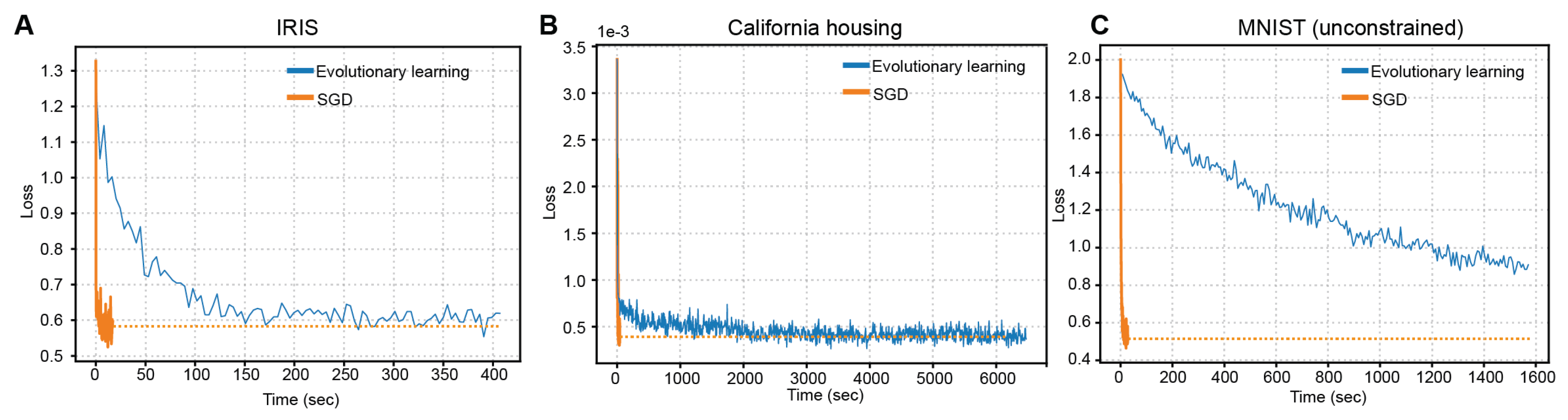
Previously, we demonstrated proposed MCNN’s model functional versatility across three benchmarks: from tabular classification and regression to high-dimensional image classification. But next foundational question emerges: how does this approach compare to the previously demonstrated [24] training methods? To evaluate this, we conducted a head-to-head comparison of our gradient-based training method against the direct evolutionary optimization approach, applying both to all three datasets. The corresponding learning curves are revealed in Figure 6A-C.

The relative efficacy of gradient- versus evolutionary-based learning hinges critically on problem scale. On the low-dimensional Iris dataset, both approaches converged to near identical accuracy, yet the backpropagation technique allowed to achieve this in under 2 seconds, whereas evolutionary search required ~150 s – a 75-fold latency despite comparable outcomes. Similar results were obtained for more complex (in terms of dimensionality and structure) California Housing regression problem, surpassing the acceleration of 24 times. Most notable advantage of gradient-driven learning is presented on the MNIST benchmark (unconstrained non-convolutional version): our method reached 92% accuracy in 27 s, while evolutionary optimization, even after ~1,540 s (57× longer), plateaued at only 70%. This emergent scaling behavior suggests a computational phase transition: beyond a critical complexity threshold, the curvature information encoded in gradients becomes indispensable for efficient navigation of high-dimensional molecular parameter spaces. The apparent contradiction with earlier reports [24], where gradients conferred little benefit, likely stems from their focus on ultra-small networks, below this threshold, where gradient signal-to-noise is low and landscape ruggedness minimal. Our results thus underline an advantage of gradient-based training for scaling biomolecular networks.

Discussion

Universality of MCNN and MCNN Training

While diverse molecular implementations of neural network models have been demonstrated in previous works, all of them lacked the generality and were locked to a narrow problem class. In contrast, our framework achieves algorithmic universality: once real-world data is linearly normalized via min-max scaling and transduced into initial oligonucleotide concentration, the entire pipeline proceeds without any task-specific tuning. The same core formalism governs a low-dimensional housing-price regressor and complex image classifier, differing only in input dimensionality and redout interpretation. This abstraction marks a critical step towards general-purpose biomolecular systems, bridging the theory between neural networks and biochemical circuits.

How Complex Can MCNN Be?

While our framework supports networks of large scale in molecular terms, it nonetheless confronts a fundamental biophysical bound: signal dampening along reaction cascades due to reversible nature of interactions. The influence of an input on an output decreases exponentially with increasing separation between them, typically becoming negligible after approximately four to five interaction steps [33] As a result, unlike artificial neural networks, MCNNs in their current state cannot be upscaled arbitrarily in depth. Therefore, further increases in computational complexity must follow alternative directions.

A natural and promising avenue is the development of modular systems – architectures in which the output of one MCNN can be physically extracted from the remaining molecular species, amplified (e.g., via enzymatic reactions), and subsequently used as the input to a second MCNN. Such modularity would enable the construction of more complex computations while simplifying the design of each individual MCNN. However, isolating specific molecular species from a mixture remains, at present, a technically challenging and labor-intensive process, thereby limiting the practical implementation of such modular architectures.

On the other hand, a simpler route to enhancing the computational capacity of MCNNs lies in enriching the complexity of individual interactions – or in incorporating alternative interaction types altogether. In this work, we restricted our focus to reversible dimerization reactions. Yet even within the paradigm of reversible binding, MCNNs could be naturally extended to include higher-order processes such as multimerization. In this case, the mass-action kinetics would transition from quadratic dependence to a higher-order power-law form (with exponent > 2). Such a change would endow specific network components with sharper, more switch-like activation dynamics, reminiscent of spiking thresholds, SwiGLU-like gating, or hard-threshold nonlinearities, which may substantially enhance the system’s capacity for nonlinear feature separation and, consequently, improve generalization performance. An even greater boost in computational capacity could be achieved by incorporating irreversible reactions (such as those catalyzed by enzymes) or by operating the system in a transient regime, where outputs are read before equilibrium is reached. Both strategies necessitate a shift from the equilibrium-based formulation of the law of mass action to its kinetic (time-dependent) counterpart.

In either scenario, training such extended MCNNs requires an explicitly defined forward pass. Fortunately, the output concentrations remain tractable and can still be computed using comparably straightforward numerical methods. For instance, finite difference schemes provide an efficient means to approximate the time evolution of species concentrations – yielding an explicit, differentiable mapping from model parameters to outputs. Consequently, the training framework introduced in this work extends naturally to these generalized architectures without fundamental modification.

Scalability and Reusability

A key limitation shared by molecular neural networks, and indeed by most biocomputing paradigms, is their inherently single-use nature: computation typically proceeds only once per reaction vessel, unless supplementary intervention (e.g., input species recycling) is explicitly implemented.

On one hand, the reversible nature of molecular interactions offers a built-in reset mechanism: removing the input species by any suitable means, effectively returns the system to an initial state, permitting the introduction of new inputs. For instance, one study [34] demonstrated chromatographic separation for input removal. Although effective, this approach is labor-intensive and poorly suited for scaling. More recently, DNA-based systems have been engineered with kinetic traps [18], enabling input clearance (and thus system reset) via a simple thermal cycling protocol (e.g., heating followed by controlled cooling), markedly improving practicality and scalability.

However, from our perspective, the true path to scalability lies in field of miniaturization – coupled with the development of novel, efficient interfaces for programming, interrogating, and controlling molecular networks. The potential for miniaturization in this field is immense. Consider a typical reaction volume of 100 µL at characteristic concentrations of 1 µM: it contains roughly 10¹⁴ molecules, all executing the same computation in parallel. Recognizing this, many current efforts aim to shrink reaction volumes down to the picoliter scale, for example, leveraging emulsion droplets as compartmentalized reactors [19], to preserve molecular parallelism while drastically reducing reagent consumption and enabling high-throughput operation. Shrinking the system to such scales allows for the generation of billions of independent, parallel microreactors – each capable of autonomously processing complex data. At this level of parallelization, reusability becomes far less essential: even a single modest-volume tube of “computational” emulsion can, in principle, analyze massive datasets simultaneously across its droplet population.

Intriguingly, this reduction in scale – from microliter-scale reactions down to pico- and femtoliter droplets (a volume decrease by a factor of 10⁶ to 10⁹) – mirrors the degree of miniaturization achieved in electronics, where devices evolved from centimeter-scale vacuum tubes to nanometer-scale transistors (a linear size decrease by a factor of ~10⁸). Yet a striking contrast remains: whereas a single transistor implements a basic logic function, an individual droplet embodies an entire molecular computational system – capable of nonlinear processing, memory-like dynamics, and collective decision-making.

Conclusion

The presented here methods of building molecular commutation neural networks bring us closer to realizing a true biomolecular CPU: a programmable, general-purpose molecular system capable of processing arbitrary information. With further progress, such systems may one day rival electronic computers in niche domains where biocompatibility, parallelism, or energy efficiency are paramount. A particularly compelling near-term application lies in diagnostics – e.g., using MCNNs to interpret complex microRNA signatures for precise, early-stage detection and stratification of cancers and other diseases. Beyond engineering, the expressive power of MCNNs also offers a fresh conceptual lens for biology itself: rather than viewing cellular signaling and regulation as linear cascades or isolated pathways, we may begin to see them as integrated, large-scale networks that collectively perform structured, nonlinear information processing on the full complement of molecular cues available to the cell. In this light, MCNNs may serve a dual purpose – not only as a scaffold for artificial biological intelligence, but also as a formal framework to decode the computational logic embedded in natural biological systems.

Materials and Methods

Parameter Scaling

To enhance numerical stability and effectively use 32-bit floating-point precision during training, K and c physical values in (M^-1 and M respectively) were scaled to a factor of 10^-5:

c_{m o d e l} = c_{p h y s} / 10^{- 5}

K_{m o d e l} = K_{p h y s} * 10^{- 5},

Where subscript “phys” designates physical units and “model” means model units.

Loss Function for Classification Tasks

Let f denote the vector of free concentrations of the output species for a given input, and let Y denote the corresponding one-hot target vector (y_i = 1 if i = argmax(f) and 0 otherwise). The training objective for the classification task is a weighted sum of three terms:

L_{task} (f, Y) = w_{CE} L_{CE} (f, Y) + w_{margin} L_{margin} (f, Y) + w_{MSE} L_{MSE} (f, Y)

First, we convert f to a probability-like vector using a temperature-scaled softmax on the logarithm of free concentrations,

P_{k} = \frac{\exp (\log (f_{k}) / T)}{\sum_{j} \exp (\log (f_{j}) / T)}

with temperature T = 0.7. This transformation has two purposes: it allows us to use standard cross-entropy loss, and it emphasizes relative rather than absolute differences in free concentrations.

Cross-entropy term. The cross-entropy is computed between P and a (optionally smoothed) target distribution Y’:

$L_{C} (f, Y) = - \sum_{k = 1}^{n_{out}} Y_{k}^{'} \log P_{k},$

Y' is obtained from the one-hot Y via label smoothing with coefficient $α$ =0.05

$Y^{'} = (1 - α) Y + \frac{α}{n_{out}} 1$

This term encourages the output species corresponding to the correct class to have higher free concentration than the others, in a way analogous to standard classifiers.
Log-margin term. To increase class separability at the level of log-concentrations, we add a margin-based penalty

$L_{margin} (f, Y) = \max (0, m + \max_{k : Y_{k} = 0} \log (f_{k}) - \sum_{k} Y_{k} \log (f_{k}))$

where m is a margin parameter (typically from 0.8 to1.4). This term penalizes situations where an incorrect class has a log-concentration close to or exceeding that of the correct class, even if the overall cross-entropy is already small. The margin term is motivated by the requirement that, in a wet-lab readout, the correct output species should remain clearly separated from all others despite measurement noise.
Mean-squared error term. Finally, we include the mean-squared error between f and the one-hot target vectors

$L_{MSE} (f, Y) = \sum_{k = 1}^{n_{out}} {(f_{k} - Y_{k})}^{2}$

This term encourages the correct output concentration to approach a high target value (normalized to 1 in model units) and all incorrect outputs to approach 0, which yields an on/off pattern that is easier to distinguish experimentally.

Sparsity Regularization

To simplify the subsequent design of DNA sequences, regularization aimed at obtaining sparse connection graphs was applied during training. This is achieved by adding a special penalty term to the loss function, which encourages each molecule to interact with only a limited number of other molecules.

For each i-th molecule in the network, a penalty is applied to all of its interactions except for the k strongest ones. The association constants

K_{i j}

themselves are used as the metric of interaction “strength.”

For each molecule i, the values K_ij are sorted in descending order. A penalty is applied to the sum of squares of all values starting from the (k + 1)-th. The total penalty for the entire network R is calculated as the average of these penalties over all species.

R = \frac{1}{n} \sum_{i = 1}^{n} \sum_{j = k + 1}^{n} {(K_{i j})}_{↓}^{2}

where

{(\cdot)}_{↓}

are the interaction strength values for the i-th molecule, sorted in descending order.

This step is integrated into the overall loss function using the training weight t.

L_{t o t a l} = L + λ (t) \cdot R

A key role in this approach is played by the scheduling of the coefficient λ(t). Applying a large value of λ from the very beginning of training would force the optimizer to immediately eliminate most connections before the model has learned to solve the main task. This approach is essentially equivalent to a naive “hard projection” at the start and generally leads to unsatisfactory results, as it restricts the model’s ability to learn.

Therefore, a warmup approach was applied. At the initial stage of training (for example, during the first 3000 steps), the coefficient λ(t) is equal to zero. During this period, the model focuses exclusively on minimizing the primary loss function L, freely adjusting all parameters to find an effective, although dense, solution. After the warmup stage, the value of λ(t) begins to increase smoothly, for example, linearly, until it reaches some maximum value.

λ (t) = \{\begin{matrix} 0, t < t_{w a r m u p} \\ λ_{m a x} \frac{t - t_{w a r m u p}}{t_{t o t a l} - t_{w a r m u p}}, t \leq t_{w a r m u p} \end{matrix}

Here, t denotes number of batches that have been evaluated. t_total is total number of batches in a dataset multiplied by total number of epochs,

Such gradual introduction of the penalty allows the model to smoothly transition from the dense solution it has found to a sparse one, while preserving the learned dependencies and “cutting off” the least important connections with minimal loss in quality. After training is completed, only the k connections with the highest weights are retained for each molecule, and all remaining association constants are forcibly set to zero.

MCNN Learning Hyperparameters

The following settings were consistent across all experiments unless explicitly overridden in the specific experiment sections.

For all gradient optimizations JAX implementation of SGD with Nesterov momentum 0.9 was used. Learning rate was scheduled as cosine decay with weight decay (L2-regularization parameter) of 10^-8. Concentrations (in scaled model units) were restricted to range [10^-4, 1].

Hyperparameter		IRIS	California housing	MNIST unconstrained	MNIST convolutional
Input Species		4	9 (8 original + 1 engineered)	196 (14x14 flattened)	729 (27x27 flattened)
Hidden Species		5	38 (Layer 1: 20, Layer 2: 18)	44	81
Output Species		3	1	10	10
K range (model units)		[ $10^{- 2}$ , $10^{5}$ ]	[ $10^{- 2}$ , $10^{6}$ ]	[ $10^{- 2}$ , $10^{10}$ ]	[ $10^{- 2}$ , $10^{6}$ ]
Effective Epochs		2000	50	10	30
Total steps		4000	3100	2350	7050
Batch Size		64	256	256	256
Solver Iterations		600	500	1000	500
Solver Damping		0.8	0.7	0.8	0.7
Loss function (weights)	Cross-Entropy	0.9	0	0.5	1
	Log-margin	0.1	0	0.1	0.1
	MSE	0.1	1	0.5	0.1
Softmax Temp / Margin		0.7 / 0.8	None	0.7 / 0.8	0.7 / 0.8
Learning Rate (K)		0.02 → 0, Cosine decay	57.79 → 0, Cosine decay	1.0 → 0, Cosine decay	1 → 0.1, Exponential decay
Learning rate (c)		0.02 → 0, Cosine decay	2.0 → 0, Cosine decay	1.0 → 0, Cosine decay	0.3 → 0.03, Exponential decay
Degree Cap ( $k_{m a x}$ )		3 (strict)	3 (strict)	None	4 (hidden-output only, non-strict)
Warmup steps		500	None	1170
Sparsity $λ$ Schedule		Linear ramp (max 10^-3)	Cubic ease-in ramp (max: 10^-4)	None	Tenfold increase each epoch (start: 10^-6, max: 10^-2)

Here, a “step” refers to the evaluation of a single batch, while an “epoch” corresponds to evaluating all batches in the dataset. For all learning-rate schedulers, decay is applied over the full sequence of training steps.

Notes for IRIS task: To stabilize the validation loss curve, the dataset epoch size was effectively multiplied by 200. The model was trained for 10 'meta-epochs', resulting in 2000 effective passes over the data.

Notes for Pseudo-Convolutional MNIST task: Connections between Input and Hidden layers were fixed to a 3x3 patch structure with stride 3. Each of the 81 hidden nodes connects to exactly 9 specific input nodes. A non-strict degree cap of k=4 was enforced on the Hidden-Output connections.

Notes for California Housing Regression: Unlike classification tasks, the output and maximum input concentrations were also optimized, optimized values are listed in Table S2.

For all four models, the complete data are provided in the supplementary file networks_data.zip in .npz format. These files contain the following fields: “K” (optimized affinity matrix, M⁻¹), “pred_K” (affinity matrix, M⁻¹, for the DNA oligonucleotides implementing the network), “c_out” and “c_hidden” (total concentrations, M, of output and hidden oligonucleotides), “meta_json” (network metadata), and “seqs” (DNA oligonucleotide sequences implementing the network).

Evolutionary Training

In addition to gradient-based training, we implemented a gradient-free evolutionary optimization procedure over the same MCNN architectures, following previous work [24].

The algorithm maintains a population of MCNNs that differ in their association matrices and concentration parameters. At each generation, all members of the population are evaluated on the same mini-batch of input patterns. For a given MCNN, the forward computation is identical to that used in the SGD experiments. Evaluations for different members of the population are parallelized across CPU cores, so that all individuals in a generation can be simulated in parallel.

The fitness of an individual is defined as the mean-squared error between the free concentrations of the output species and the one-hot target vectors on the mini-batch. After each generation, the individual with the lowest loss is compared with the current parent. A simulated-annealing acceptance rule is applied: if the candidate has lower loss, it is always accepted; if it has higher loss, it is accepted with probability exp(−∆L/T), where ∆L is the increase in loss and T is a temperature parameter. The temperature is decreased geometrically from 1.0 to 0.2 over the course of training, which gradually reduces the probability of accepting worse candidates.

New offspring are generated by mutating the accepted parent. For each child, the current association constants are perturbed multiplicatively by independent log-normal factors,

K_{i j}^{child} = clip (K_{i j}^{parent} \exp (ϵ_{i j}), K_{m i n}, K_{m a x}), ϵ_{i j} \sim N (μ, σ^{2})

μ

= -0.04 and σ = 0.5 in the experiments below. The same structural constraints and regularization as in the SGD experiments are then re-applied.

Hidden-species concentrations are mutated by multiplying each component by a uniform random factor in the range [0.9; 1.1] and clipping the result to [10^-4; 1.0]. Output-species concentrations are mutated more conservatively with factors in [0.95; 1.05] and the same clipping. Thus, each generation explores a local neighborhood of the current parent in both affinity and concentration space, while always respecting the imposed physicochemical bounds and topological constraints.

NUPACK Predictions

The NUPACK package for the Python programming language (version 4.0.1.12) was employed in this study. The method for computing equilibrium constants was adapted from the original publication describing the fundamental algorithms of the service [35]:

K = c_{H_{2} O} \frac{Z_{s 1} Z_{s 2}}{Z_{s 1 s 2}}

where the indices s1 and s2 refer to the interacting oligonucleotides, Z denotes the partition function of the respective complex, and

c_{H_{2} O}

is the molar concentration of water. The partition function was computed as the pfunc attribute of the nupack.complex_analysis object. In all calculations, the maximum number of complexes parameter was set to 2.

Evolutionary Sequence Finding Using Trained MCNN Graph

After obtaining optimized association constants via gradient-based optimization, sequence search was performed. The association constant matrix K_ij was interpreted as a graph: an edge between molecules i and j was included if K_ij > K_thr, with K_thr typically set to 10⁵ M⁻¹. Each K_ij was then converted to the corresponding Gibbs free energy:

G = - R * T * l n (K)

A virtual node was added to the graph, connected by virtual edges only to the output molecules. Sequences were then identified one by one using breadth-first search starting from this virtual node. For the first node, the sequence was chosen randomly.

The procedure for identifying the (N+1)-th sequence assumed that N sequences had already been found. The (N+1)-th sequence had to satisfy N+1 constraints: its Gibbs free energies of binding to all existing oligos had to be sufficiently close to the target values encoded in the graph edges (N constraints), and its self-binding energy had to be sufficiently low. If no edge existed between the new molecule and a previously identified one, the corresponding constraint required that the Gibbs free energy be greater than or equal to a threshold G_thr, typically set to −30 kJ/mol. The same constraint applied to self-interaction.

From these N molecules, those with target binding energies above G_thr were designated as target oligos. Desired oligo lengths were set to 20 nucleotides for the IRIS and California Housing datasets, and 30 nucleotides for MNIST. All remaining oligos were treated as off-targets. Sequences reverse-complementary to the target oligos were subjected to a random truncation (0–15 nucleotides). The initial candidate for the (N+1)-th oligo was constructed as a random mosaic of subsequences drawn from all truncated oligos, using one subsequence per truncated oligo.

The DEAP library [36] was then used to perform evolutionary refinement of the (N+1)-th oligo through random mutations (1–3 nucleotides per step) and crossover with other sequences in the population. Typical parameters were: population size 200, 20 generations, mutation probability 0.5, crossover probability 0.5. Early stopping was triggered when the total deviation between target and inferred by NUPACK Gibbs energies reached approximately 5–7 kJ/mol.

If the algorithm failed to find a sequence satisfying the constraints, the algorithm continued to the next sequence.

Supplementary Materials

The following supporting information can be downloaded at the website of this paper posted on Preprints.org.

Author Contributions

A.A.Z., N.R.B., R.A.M. developed the theory, developed the code for gradient optimization, conducted in silico experiments. E.S.K. and A.M.V. developed the sequence finding algorithms. A.A.Z., R.A.M., N.R.B., A.M.V. and E.S.K. visualized the data. E.S.K. and N.R.B. wrote the original draft. M.P.N. and A.N.B. supervised the project. M.P.N. conceptualized the study, acquired funding. All authors participated in manuscript editing and curation.

Declaration of interests

M.P.N. is the inventor and the applicant of a related patent application RU2756476C2.

Declaration of generative AI and AI-assisted technologies in the writing process

During the preparation of this work the authors used generative AI in order to translate parts of the original draft from Russian into English. After using this tool, the authors reviewed and edited the content as needed and take full responsibility for the content of the published article.

Acknowledgments

This research was supported by the Ministry of Science and Higher Education of the Russian Federation agreement 075-03-2025-662, project FSMG-2023-0017.

References

Stiefel, K. M. & Coggan, J. S. The energy challenges of artificial superintelligence. Front Artif Intell 6, (2023). [CrossRef]
Badia-i-Mompel, P. et al. Gene regulatory network inference in the era of single-cell multi-omics. Nat Rev Genet 24, 739–754 (2023). [CrossRef]
Tay, Y., Rinn, J. & Pandolfi, P. P. The multilayered complexity of ceRNA crosstalk and competition. Nature 505, 344–352 (2014). [CrossRef]
Antebi, Y. E. et al. Combinatorial Signal Perception in the BMP Pathway. Cell 170, 1184-1196.e24 (2017). [CrossRef]
Cardelli, L. & Csikász-Nagy, A. The Cell Cycle Switch Computes Approximate Majority. Sci Rep 2, 656 (2012). [CrossRef]
Adleman, L. M. Molecular Computation of Solutions to Combinatorial Problems. Science (1979) 266, 1021–1024 (1994). [CrossRef]
Seelig, G., Soloveichik, D., Zhang, D. Y. & Winfree, E. Enzyme-Free Nucleic Acid Logic Circuits. Science (1979) 314, 1585–1588 (2006). [CrossRef]
Nikitin, M. P. Non-complementary strand commutation as a fundamental alternative for information processing by DNA and gene regulation. Nat Chem 15, 70–82 (2023). [CrossRef]
Katz, E. & Privman, V. Enzyme-based logic systems for information processing. Chem Soc Rev 39, 1835 (2010). [CrossRef]
Guo, Z. et al. Development of e pistatic YES and AND protein logic gates and their assembly into signalling cascades. Nat Nanotechnol 18, 1327–1334 (2023). [CrossRef]
Mao, C., LaBean, T. H., Reif, J. H. & Seeman, N. C. Logical computation using algorithmic self-assembly of DNA triple-crossover molecules. Nature 407, 493–496 (2000). [CrossRef]
Yang, J., Jiang, S., Liu, X., Pan, L. & Zhang, C. Aptamer-Binding Directed DNA Origami Pattern for Logic Gates. ACS Appl Mater Interfaces 8, 34054–34060 (2016). [CrossRef]
Nikitin, M. P., Shipunova, V. O., Deyev, S. M. & Nikitin, P. I. Biocomputing based on particle disassembly. Nat Nanotechnol 9, 716–722 (2014). [CrossRef]
Cherkasov, V. R., Mochalova, E. N., Babenyshev, A. V. & Nikitin, M. P. All-in-one Biocomputing Nanoagents with Multilayered Transformable Architecture based on DNA Interfaces. Theranostics 15, 8451–8472 (2025). [CrossRef]
Jia, S., Lv, H., Li, Q., Fan, C. & Wang, F. DNA-based biocomputing circuits and their biomedical applications. Nature Reviews Bioengineering 3, 535–548 (2025). [CrossRef]
Qian, L., Winfree, E. & Bruck, J. Neural network computation with DNA strand displacement cascades. Nature 475, 368–372 (2011). [CrossRef]
Cherry, K. M. & Qian, L. Scaling up molecular pattern recognition with DNA-based winner-take-all neural networks. Nature 559, 370–376 (2018). [CrossRef]
Song, T. & Qian, L. Heat-rechargeable computation in DNA logic circuits and neural networks. Nature 646, 315–322 (2025). [CrossRef]
Okumura, S. et al. Nonlinear decision-making with enzymatic neural networks. Nature 610, 496–501 (2022). [CrossRef]
Ghosh, S. et al. A recursive enzymatic competition network capable of multitask molecular information processing. Nat Chem (2025) . [CrossRef]
Nikitin, M. P. Molecular computing device based on essentially non-complementary single stranded nucleic acids with low mutual affinity. (2021).
Parres-Gold, J., Levine, M., Emert, B., Stuart, A. & Elowitz, M. B. Contextual computation by competitive protein dimerization networks. Cell 188, 1984-2002.e17 (2025). [CrossRef]
Sun, C., Liu, X., Zhong, J., Zhou, Q. & Cheng, J. A Reusable Non-Complementary-DNA-Based Neural Network. (2024).
Tkachenko, A. V., Mognetti, B. M. & Maslov, S. Evolutionary chemical learning in dimerization networks. http://arxiv.org/abs/2506.14006 (2025).
Cai, H., Zhang, X., Qiao, R., Wang, X. & Wei, L. Efficient computation by molecular competition networks. Phys Rev Res 6, 033208 (2024). [CrossRef]
Feinberg, M. Chemical reaction network structure and the stability of complex isothermal reactors—I. The deficiency zero and deficiency one theorems. Chem Eng Sci 42, 2229–2268 (1987). [CrossRef]
van Dorp, M. G. A., Berger, F. & Carlon, E. Computing equilibrium concentrations for large heterodimerization networks. Phys Rev E 84, 036114 (2011). [CrossRef]
Izmailov, S. A., Podkorytov, I. S. & Skrynnikov, N. R. Simple MD-based model for oxidative folding of peptides and proteins. Sci Rep 7, 9293 (2017). [CrossRef]
Zadeh, J. N. et al. NUPACK: Analysis and design of nucleic acid systems. J Comput Chem 32, 170–173 (2011). [CrossRef]
Fornace, M. E. et al. NUPACK: Analysis and Design of Nucleic Acid Structures, Devices, and Systems. (2022). [CrossRef]
Korenkov, E. S. & Nikitin, M. P. Topology of molecular networks offers signaling insusceptibility to temperature and ionic strength changes. bioRxiv 2025.10.09.680621 (2025). [CrossRef]
Li, H., Xu, Z., Taylor, G., Studer, C. & Goldstein, T. Visualizing the Loss Landscape of Neural Nets. (2018).
Maslov, S. & Ispolatov, I. Propagation of large concentration changes in reversible protein-binding networks. Proceedings of the National Academy of Sciences 104, 13655–13660 (2007). [CrossRef]
Sun, C., Liu, X., Zhong, J., Zhou, Q. & Cheng, J. Reusable Noncomplementary DNA-Based Neural Network. J Am Chem Soc 147, 34339–34349 (2025). [CrossRef]
Dirks, R. M., Bois, J. S., Schaeffer, J. M., Winfree, E. & Pierce, N. A. Thermodynamic Analysis of Interacting Nucleic Acid Strands. SIAM Review 49, 65–88 (2007). [CrossRef]
Fortin, F.-A., De Rainville, F.-M., Gardner, M.-A., Parizeau, M. & Gagné, C. DEAP: Evolutionary Algorithms Made Easy. Journal of Machine Learning Research 13, 2171–2175 (2012).

Figure 1. MCNN concept. (A) Encoding and processing of information in an MCNN. (B) MCNN training scheme. (C) Algorithmic workflow for finding sequences that implement the MCNN. (D) Sparsity regularization demonstration.

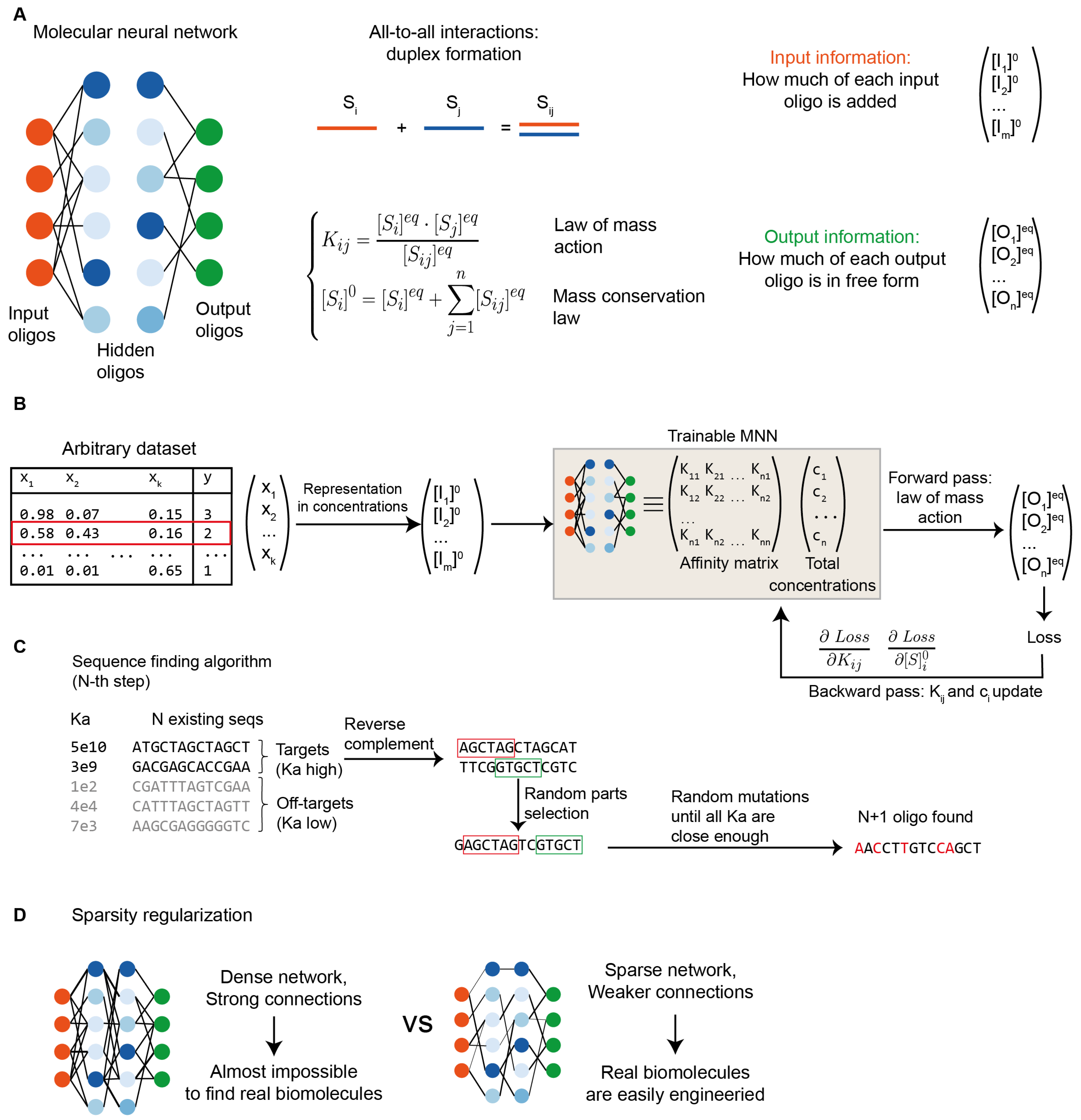
Figure 2. MCNN for the IRIS dataset. (A) MCNN learning curve. (B) Interaction graph of oligonucleotides in the MCNN and their sequences. Edge thickness is proportional to the logarithm of the association constant. (C) MCNN confusion matrix. (D) Distribution of the concentrations of the three output oligonucleotides when inputs corresponding to different true classes are supplied. The outputs corresponding to the true class are highlighted in green or red. A point is highlighted in green if the predicted class matches the true one, and in red otherwise.

Figure 3. MCNN for the California Housing dataset. (A) Learning curve. (B) Loss function landscape [32]. Direction 1 (x) and Direction 2 (y) are two randomly chosen orthogonal vectors defining a two-dimensional slice of the network’s multidimensional parameter space. Movement along these axes corresponds to the simultaneous perturbation of all association constants and concentrations in the model by a random amount proportional to their current values. (C) Interaction graph of oligonucleotides in the MCNN and their sequences. Edge thickness is proportional to the logarithm of the association constant. (D) Scatter plot of predicted versus true values.

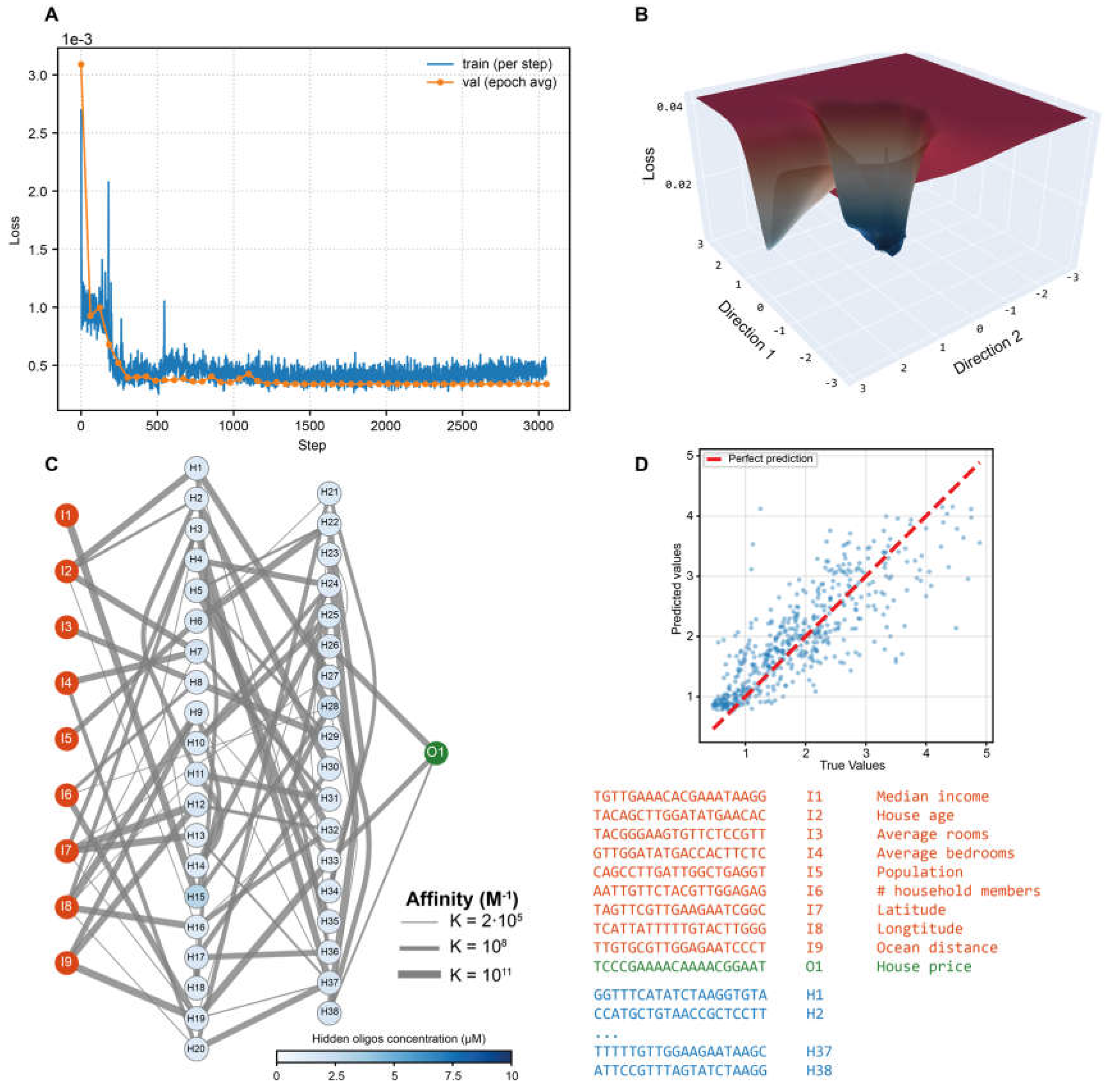
Figure 4. Pseudo-convolutional MCNN for the MNIST dataset. (A) Schematic representation of the network. (B) MCNN learning curve. (C) Pruned interaction graph of oligonucleotides in the MCNN and selected sequences. Edge thickness is proportional to the logarithm of the association constant. (D) Importance map for two selected samples. Importance is defined as the absolute value of partial derivative of the corresponding output oligo with respect to the concentration of each input oligo (i.e., pixels).

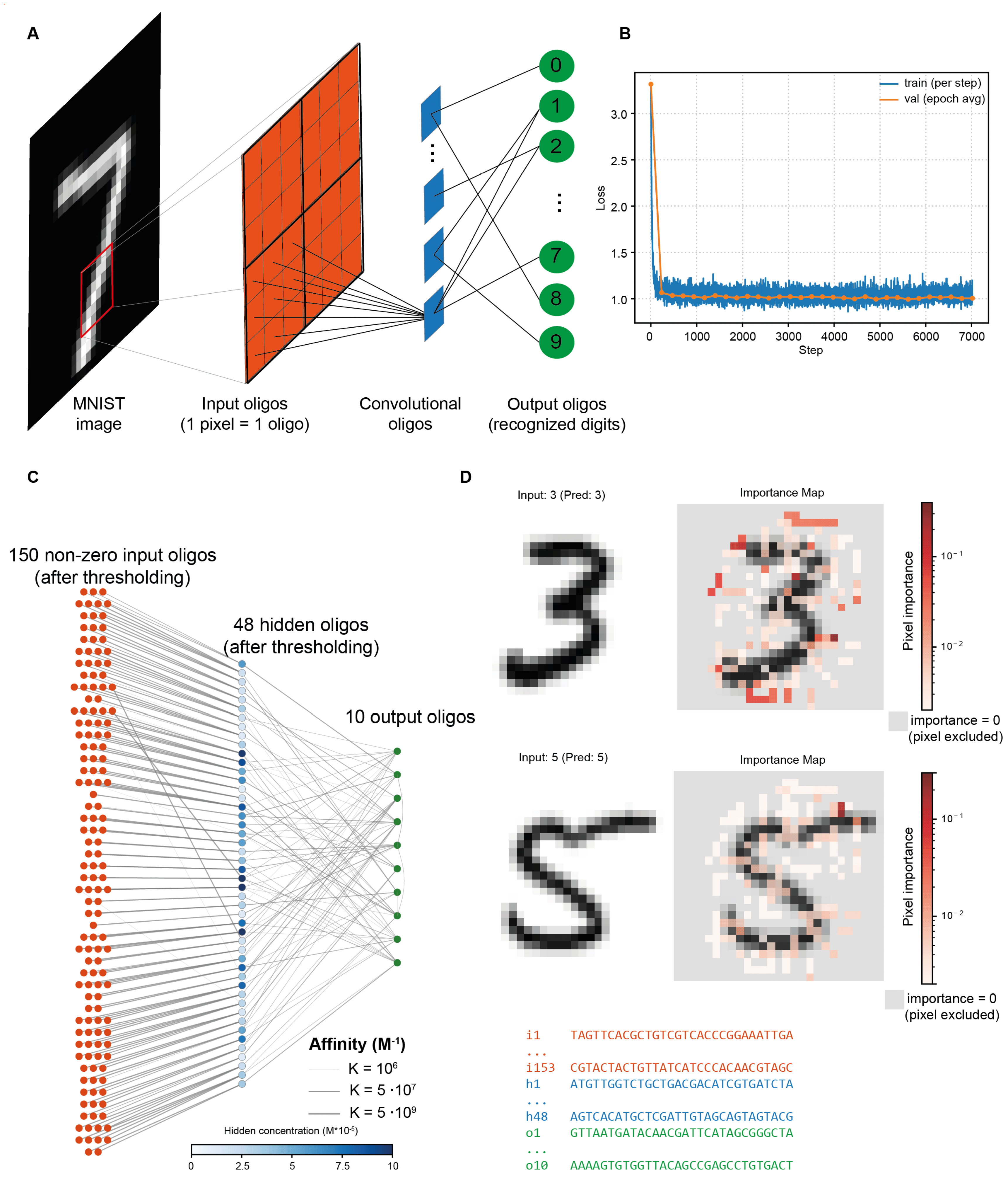
Figure 5. Performance of the pseudo-convolutional MCNN. (A) Confusion matrix. (B) Distribution of the equilibrium concentrations of the output oligos when samples corresponding to the digit 0 (test set) are fed into the system. (C) Same distributions for all digits as violin plots.

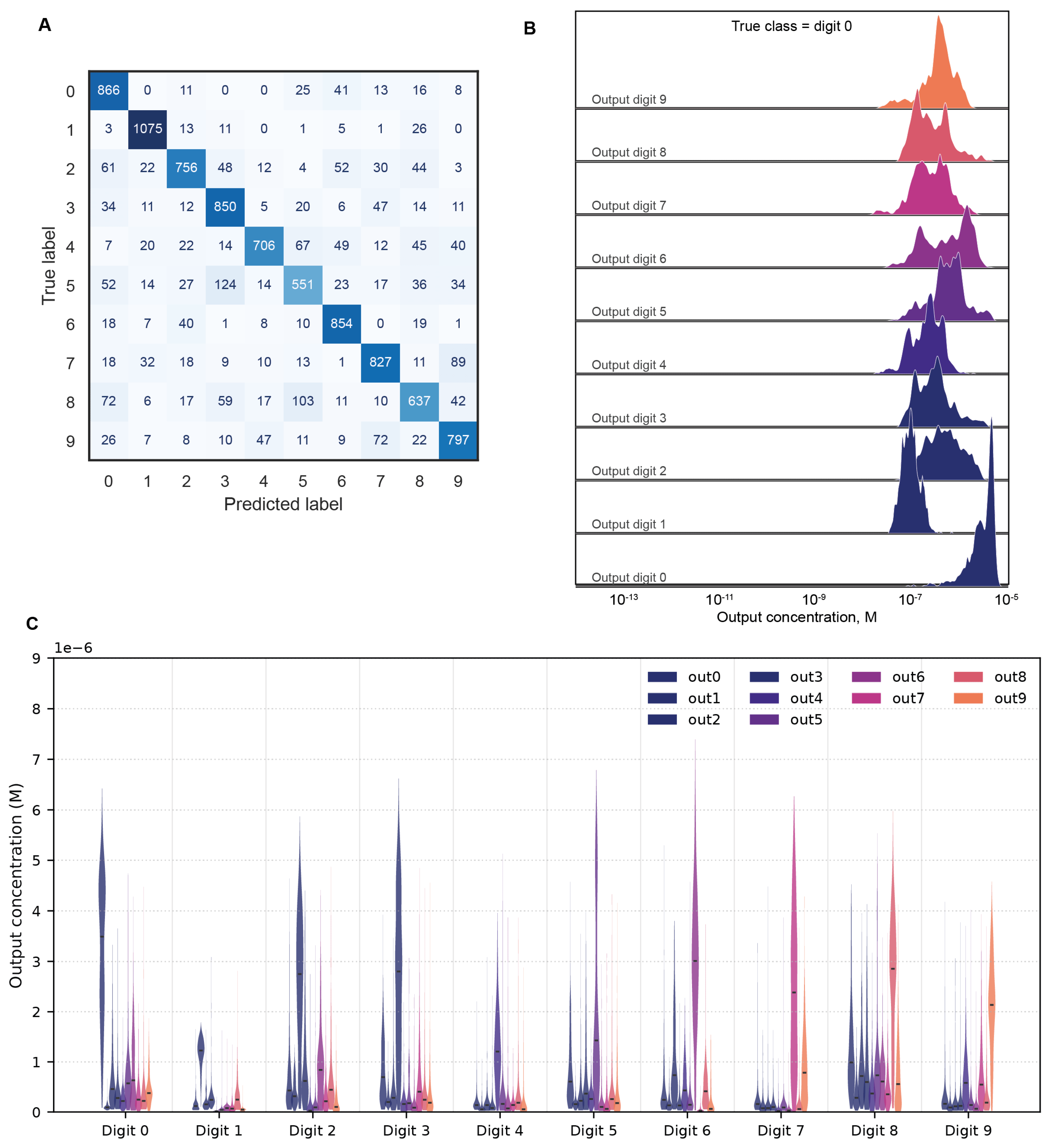
Figure 6. Comparison of gradient-based and evolutionary training methods. (A–C) Learning curves of MCNNs for the IRIS, California Housing, and MNIST datasets, respectively, trained using either SGD or an evolutionary algorithm.

Disclaimer/Publisher’s Note: The statements, opinions and data contained in all publications are solely those of the individual author(s) and contributor(s) and not of MDPI and/or the editor(s). MDPI and/or the editor(s) disclaim responsibility for any injury to people or property resulting from any ideas, methods, instructions or products referred to in the content.

© 2026 by the authors. Licensee MDPI, Basel, Switzerland. This article is an open access article distributed under the terms and conditions of the Creative Commons Attribution (CC BY) license (http://creativecommons.org/licenses/by/4.0/).

Copyright: This open access article is published under a Creative Commons CC BY 4.0 license, which permit the free download, distribution, and reuse, provided that the author and preprint are cited in any reuse.