
Submitted:
30 October 2025
Posted:
31 October 2025
You are already at the latest version
Abstract
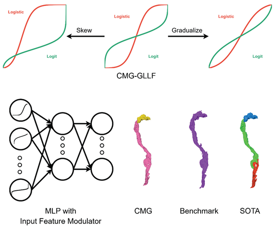
Logistic and logit functions play important roles in modern science, serving as foundational tools in various applications including artificial neural network (ANN). While there are functions that could produce distinct logistic and logit curves, no single, unified framework has been developed to generate both logistic and logit curves. We introduce a generalized logistic–logit function (CMG-GLLF) to fill this gap. CMG-GLLF provides four interpretable and trainable parameters that allow explicit control over: curve type and steepness, asymmetry, upper and lower limits of x- and y-axes. CMG-GLLF’s potential is explored in basic machine intelligence tasks. We propose a trainable input feature modulator (IFM) for multi-layer perceptron (MLP) that consists in learning the parameters of the CMG-GLLF for each input layer node during backpropagation, achieving MLP’s superior accuracy and faster learning speed in image classification. Furthermore, CMG-GLLF as data transformation enhances the accuracy of affinity-graph-based neuron segmentation. CMG-GLLF combines in a unique framework the ability of logistic and logit function to modulate signals or variables, covering a full spectrum of attenuation or amplification transformations. CMG-GLLF is flexible and trainable, has potential to advance machine learning models, and can inspire further applications in other data analysis challenges in different domains of science.
Keywords:
generalized logistic–logit function
; input feature modulator
; neural networks
; multi‐layer perceptron
; neuron segmentation
1. Introduction
Logistic and logit functions play pivotal roles in various fields such as economics, medicine and computer science.[1], [2], [3], [4] The logistic function is a fundamental mathematical tool widely employed across diverse fields due to its unique S-shaped curve and bounded output. In statistics and machine learning, it forms the core of logistic regression, enabling effective modeling of binary outcomes and probabilistic predictions.[5], [6] In biology, the logistic function is used to describe growth phenomena under resource constraints, capturing the transition from exponential growth to saturation.[7], [8] Its smooth, differentiable nature also makes it indispensable in artificial neural networks, where it serves as a nonlinear activation function facilitating gradient-based learning.[4] Meanwhile, the logit function, the inverse of the logistic function, maps probabilities from the interval (0,1) onto the entire real line by transforming a probability p into its log-odds. This transformation is central to logistic regression: by modeling the log-odds in terms of predictors, the logit function allows one to capture how the linear combination of covariates and predictors affects the probability of event happening.[5] The versatility of the logistic and logit functions in modeling growth, decision-making, classification, and intelligent systems underscores their enduring significance in both theoretical and applied research.
Nevertheless, the standard logistic and logit functions expressed as
has limited flexibility, which restricts their ability to capture complex real-world phenomena—particularly in cases of imbalanced, skewed, or asymmetric growth and response behaviors. To overcome these shortcomings, researchers have introduced generalized logistic (Richards curve) and generalized logit functions with additional tunable parameters, thereby extending their adaptability to a wider range of scientific applications.[9], [10] (See Supporting Information A for detailed description) Yet, these approaches still face important limitations:
- (1)
- Lack of exact boundaries. Generalized logistic and logit functions do not provide exact reachable lower and upper bounds on either the x- or y-axis, posing difficulties in applications that require strict input/output boundaries and precise mappings. For example, when modeling the relationship between project time t and completion rate r: at the start (t=0), r=0%, and values below this have no practical meaning; at the deadline (t=T), r=100%, and values beyond this point are impossible.
- (2)
- Limited shape control. The steepness and asymmetry of generalized logit functions are determined only by the relative relationship between two parameters, instead of using separate parameters that independently control these curve characteristics.
To address these issues, we introduce the Cannistraci–Muscoloni-Gu generalized logistic–logit function (CMG-GLLF, denoted as CMG below for simplicity), which not only fills these gaps but also provides the first unified framework for generating both generalized logistic and logit curves. Derived from generalized logistic function (Richards curve),[9] CMG offers:
- (1)
- Explicit control over exact reachable lower and upper bounds on both x and y axis
- (2)
- Independent control of steepness and asymmetry through inflection rate and deviate inflection point.
- (3)
- An approximation algorithm to derive the logit curve by inverting the generalized logistic curve, introducing more flexibility into logit curve.
- (4)
- A unifying inflection rate parameter that enables smooth transitions between step functions, logistic functions, linear functions, and constant functions.
We explore CMG’s potential in machine learning through two main applications. First, we investigate its use as an input feature modulator (IFM), assigning each input feature a CMG curve with learnable parameters (via gradient update in back propagation) to enhance multi-layer perceptron (MLP) performance in terms of both best accuracy and faster learning speed. Second, we demonstrate that CMG can improve the accuracy of an affinity-graph-based neuron segmentation algorithm by transforming affinity graphs with CMG mappings.[11]
Overall, CMG provides a powerful new family of input feature modulators and data transformation tools for machine learning. With its high flexibility, optimized CMG’s curves can be tailored to diverse tasks thereby they might be investigated in future studies for accelerating the deployment of machine learning models in both research and industry.
2. Results and Discussion
2.1. CMG
The expression of CMG is given by
The below text and Figure 1 explain how different parameters affect the shape of CMG curve.
- and are the minimum and maximum of x values
- and are the corresponding y value of and
- is deviate inflection point determining the asymmetry of the curve and controls the relative position of it on x-axis, specifically
- ○
- when , the curve is left-skewed
- ○
- when , the curve is symmetric about the deviate inflection point
- ○
- when , the curve is right-skewed
- ○
- is inflection rate controlling the steepness and the type of CMG curve, specifically:
- ○
- When , the curve is a step function
- ○
- When 0<μ<0.5, it is a logistic curve, and a lower μ results in a steeper curve
- ○
- When μ=0.5, it is a linear curve
- ○
- When 0.5<μ<1, it is a logit curve derived from an approximation algorithm that inverts the logistic curve, and a lower μ results in a steeper curve.
- ○
- When μ=1, it becomes a constant function defined as
The derivation of CMG and the approximation algorithm can be found in Supporting Information B.
2.2. CMG as MLP Neural Network Input Feature Modulator (IFM)
The goal of this section is to offer evidence that CMG is trainable. To this aim we demonstrate that by applying CMG as input feature modulator for MLP in image classification, the accuracy and learning speed can be greatly improved. The motivation to design an IFM is the hypothesis that task-oriented learning of the input feature value distribution during end-to-end training provides a better representation of input data to improve the model’s performance. Specifically, we assign each input feature a learnable CMG curve during end-to-end training to modulate (amplifying or attenuating) the feature values. During training, μ and I can be learned within the limit of definition range (0<μ<1, 0<I<1). This means that the MLP has 2*Ni parameters more to train, where Ni is the number of nodes in the input layer. The upper and lower limits of x- and y-axes are data specific, in which the lower bound for x and y values are minimal value in the input data batch, and the upper bound is the maximal value in input batch. This is to ensure only the value distribution is reshaped but the original feature range is kept invariant.
We focus on MLP for image classification rather than on more recent and complex neural network architectures, because MLP represents one of the simplest network forms and are therefore well suited to evaluate the net effect of the IFM, avoiding interference from other performance-enhancing mechanisms such as convolutional layers.[12], [13] In addition, we conducted an extensive set of experiments to evaluate multiple CMG training scenarios and to compare them with other transformation functions; therefore, we opted for the MLP to moderate GPU computing costs.
We train the CMG on the MLP as a stress test to cope with two image classification tasks that are difficult for a basic neural network architecture: CIFAR-10 (in which the task is to classify a colored 32x32 image into one of the 10 object categories) and CIFAR-100 (similar to CIFAR-10 but there are 100 object categories, which is more challenging ).[14] For CIFAR-10 we adopt an MLP with 2 hidden layers with size {1024,512} as done by Wesselink et al, [15] This means that for CIFAR-10 the IFM costs a 0.17% (2*Ni/total number of parameters = 2*3072/ ((3072 * 1024) + 1024+(1024 * 512) + 512+(512 * 10) + 10+2*3072)) parameter increase. For CIFAR-100 we extend the hidden layer dimension by 2 to enable the network dealing with a more complex task.[15] This means that for CIFAR-100 the IFM costs a 0.07% (2*Ni/total number of parameters = 2*3072/ ((3072 * 2048) + 2048 +(2048 * 1024) + 1024+(1024 * 100) + 100 + 2*3072)) parameter increase. Figure 2A depicts the MLP with input feature modulator in the input layer. We also extended the number of training epochs in Wesselink et al from 100 to 150 for a deeper investigation of IFM’s potential.[15] The training configurations are described in Section 4.3.
In the experiments, the highest accuracy in all epochs is taken to measure the classification performance and area across epochs (AAE) proposed in Zhang et al is utilized to measure the learning speed (calculation detailed in Section 4.6).[16]
In ANN training, learning rate scheduler is widely applied to gradually decay the learning rate as training proceeds, which enable a smooth transition from exploration at the beginning and exploitation in the end.
Here we investigate 3 learning rate (LR) schedulers with different decay patterns to determine which one works best on MLPs with CMG input feature modulator (CMG) and without IFM (original MLP). Here linear scheduler decays linearly, while sub-linear scheduler decays faster at first and then gradually reduce the decay speed, and supra-linear scheduler has the inverse tendency of sub-linear scheduler. After training for 90% of total epochs, the learning rate for 3 schedulers converge at the same point and remain the same for the rest of the training. The detailed formulas for the schedulers are provided in Method section 4.2. Figure 2B depicts the learning rate decay of 3 schedulers in 150 epochs with
We evaluated these 3 schedulers on CIFAR100 (the most complicated task in the study) to determine which works best and the results shown in Figure 2C reveals that supra-linear scheduler has the best accuracy and AAE in both CMG and original MLP. Thus, supra-linear scheduler is employed in all the following experiments.
Furthermore, to show the performance boost brought by CMG is not simply from increasing the number of parameters in the network, we tested 4 other learnable functions with 2 tunable parameters as its counterpart for a fair comparison (Detailed in Supporting Information D) and CMG was the best performing. Not still satisfied, to foster a deeper and complete research, we tested whether CMG can outperform learnable functions with more than 2 parameters, comparing CMG against a 4-parameter learnable function SReLU.[17] (Detailed in Supporting Information E)
Figure 2D and 2E show the accuracy of MLP modulated by CMG, linear transformation (best-performance counterpart function), and original MLP on test sets across the epochs for CIFAR10 and CIFAR100 respectively. As can be seen here across both datasets:
- By adopting CMG as IFM, we can greatly improve both the accuracy and learning speed compared to the original MLP. On CIFAR10 (fig. 2D) and CIFAR100 (fig.2E), we achieve an absolute improvement of 5.04% and 6.38% compared to original MLP. Also, adopting CMG can increase AAE for 3.93% and 5.81% on CIFAR10 and CIFAR100 respectively
- Among the five different 2-parameter IFM functions, CMG achieves both the best accuracy and highest learning speed followed by linear transformation function (Supporting Information D)
- Compared against SReLU, a 4-parameter IFM function, CMG has higher learning speed on both datasets, and it achieves superior accuracy on CIFAR-10 and comparable accuracy on CIFAR-100. (Supporting Information E)
Furthermore, to gain a better understanding of how CMG improves the learning, we visualize the test set image of CIFAR10 before and after CMG modulation in Figure 3, where the learned IFM with best accuracy is adopted. Taking category “frog” and “bird” as examples, it could be observed that after CMG modulation, there is a clearer brightness contrast in the image. For example, the important features such as the eye of the frog and the crest of the bird are more highlighted after modulation. To quantitatively validate this phenomenon, for each image, luma[18] (a proxy for measuring brightness, higher the brighter) of each pixel is calculated. By calculating root mean square (RMS) of lumas in the image, the extent of brightness contrast can be measured. [19] The RMS Contrast (Luma) bar plot in Figure 3 shows that the brightness of pixels is more dispersed after CMG modulation, indicating IFM provides a stronger brightness contrast after modulation. The methods to calculate luma and RMS are described in Section 4.5
2.3. Improving Affinity-Graph-Based Neuron Image Segmentation Algorithm with CMG
In this section, we demonstrate the effectiveness of CMG in improving the accuracy of an algorithm that segment neurons in brain electron microscopy (EM) images. Here we utilize the re-aligned, augmented Drosophila brain EM 3D image from CREMI challenge as benchmark dataset and CREMI score as evaluation metric (detailed in Section 4.6). [20] The segmentation pipeline proposed by Funke et al is adopted as SOTA method. (see Figure 4A).[11] Specifically, the pipeline first predicts an affinity graph for the 3D brain image, which estimates the probability that each pair of adjacent voxels in the image belongs to the same neuron segment (referred as the original affinity graph here). We can enhance the sharpness of the affinity graph weights by increasing their contrast with the CMG that acts as a soft thresholding transformation. Then an aggregation algorithm merges the voxels into neuron segments based on the affinity graph weight values, which involves 2 segmentation parameters: merge function (MF) and a thresholding parameter.
Here the motivation to apply CMG as a data transformation tool is to adjust the weight value distribution in the original affinity graph, resulting in transformed affinity graphs, aiming to improve the accuracy of final segmentation. A grid-search is performed on a range of different CMG parameters to determine the optimal combination of inflection rate (μ) and inflection point (I) for enhancing segmentation performance. The upper and lower limits are data specific and are fixed at the minimal and maximal affinity values in the affinity graph to reshape only the distribution of values but keep the affinity value range invariant. For each affinity graph including both transformed and the original, a grid-search involving 5 different merge functions and 9 thresholds are applied to produce the segmentations. Table 1 shows the grid-search space for neuron segmentation experiments. For both the original and transformed affinity graph, the segmentation that yields the lowest CREMI score, is used to represent the performance of the state-of-the-art (SOTA) and CMG-enhanced SOTA (denoted as CMG-enhanced here) respectively.
Compared to the SOTA method proposed by Funke et al. [2], CMG-enhanced shows a clear improvement in neuron segmentation quality. As shown in Figure 4B, and 4C, when μ=0.4 and I = 0.3, the segmentation result produced using the transformed affinity graph achieves a CREMI score that is 9.0% lower than that of the original affinity graph.
Additionally, we conduct a qualitative evaluation of neuron segmentations produced with different methods (Figure 4D). In the middle is a neuron segment in CREMI benchmark. Its corresponding neuron segments in CMG-enhanced segmentation is made of 2 segments with the pink one below preserving most of the structures in the benchmark. While those in SOTA segmentation is more fractured which splits the neuron segments in 3 parts, which causes more split errors.
3. Conclusions
We developed the Cannistraci–Muscoloni-Gu generalized logistic–logit function (CMG-GLLF), the first unified framework capable of generating both logistic and logit curves. Its tunable parameters enable flexible control over curve type, steepness, asymmetry, and the upper and lower limits on both the x- and y-axes.
By assigning each feature a learnable CMG curve as input feature modulator (IFM) during backpropagation, we greatly improved the performance of fully connected MLPs with a negligible parameter increase (0.17% in CIFAR-10 and 0.07% in CIFAR-100), achieving superior accuracy and faster learning speed compared with other trainable functions. Moreover, the CMG curve enhanced the accuracy of a neuron image segmentation algorithm by transforming its intermediate product—the affinity graph. These experiments demonstrate that CMG, as a simple yet flexible computational tool, holds promise for advancing machine learning models.
Despite these advantages, CMG has certain limitations. First, we deliberately chose not to use CMG as an activation function. In the input layer, where images are normalized, the bounds of x and y values remain stable, making CMG well-suited as an IFM. In contrast, activation values of hidden layers typically fluctuate during training, which may make the shape of CMG curve varies a lot from batch to batch because of the instable lower and upper bounds of input values. A solution to this issue should be devised in future studies to adopt CMG as activation function. Second, logit curves are obtained by approximating the inverse of logistic curves, which lack explicit analytical expressions. Consequently, gradients during backpropagation for the logit-phase CMG-GLLF is currently approximated. Third, interpreting the deviate inflection point in CMG presents challenges. In classical logistic curves, the inflection points mark the location of maximum growth rate. However, because CMG introduces the parameter Q to control bounds on both axes, inflection point becomes deviated, which means it aligns with the maximum growth rate only when I=0.5. Although our definition of deviate inflection point remains a useful reference for curve behavior, it introduces deviations that should be carefully considered when applying CMG to specific tasks where the position of maximum growth rate is extremely important. Finally, we deliberately chose to test the CMG as input feature modulator on the MLP in image classification because it is well suited to evaluate the net effect of the IFM (avoiding interference from other performance-enhancing mechanisms such as convolutional layers) and to contain GPU computing costs.
In this article, we mainly explored CMG’s applications in basic AI. Looking ahead, its potential should be tested in other domains of AI where more complicated neural network architectures and tasks could benefit of an input feature modulator. Furthermore, CMG’s potential can extend to other domains of data science, such as logistic regression and growth analysis, where the ability to generate both logistic and logit curves could be further explored.
4. Methods
4.1. Datasets
Here CIFAR-10 and CIFAR-100 datasets are adopted as benchmark image classification datasets for evaluating the performance of input feature modulator. [14] Both of them consists of 32×32 colored images. CIFAR-10 contains 60,000 images evenly distributed across 10 classes, while CIFAR-100 contains the same number of images but divided into 100 classes with 600 images per class. Each dataset is split into 50,000 training and 10,000 test images.
For neuron segmentation, publicly available Drosophila melanogaster brain electron microscopy (EM) image dataset from MICCAI 2016 CREMI Challenge is adopted here to show the effectiveness of CMG in improving the accuracy of automatic neuron segmentation algorithm.[11] Our experiment utilizes re-aligned augmented CREMI training set B provided in Funke et al as benchmark. [11] The ground-truth labeling provided is an instance segmentation of neurons in 3D images, where voxels sharing the same neuron label belongs to the same neuron segment.
4.2. Learning Rate Schedulers
For a deeper investigation of how different learning rate decay patterns can impact the training of MLP with input feature modulator, we designed 3 different learning rate schedulers, in which linear scheduler decays linearly, while sub-linear scheduler decays faster at first and then gradually reduce the decay speed, and supra-linear scheduler has the inverse tendency of sub-linear scheduler. Their expressions are detailed below:
Denoting as current learning rate, as initial learning rate, as total number of epochs, and as current epoch
- Linear scheduler
- Sub-linear scheduler
- Supra-linear scheduler
4.3. IFM Training Setups
Here to evaluate the performance of IFM, we adopted MLP to train on 2 popular benchmark image classification tasks: CIFAR-10 and CIFAR-100.
In all cases we have used the same training method and hyper-parameter grid-search space listed in Table 2.
The only difference between trials is the network scale. For CIFAR-10 we adopt the MLP proposed in Wesselink et al where there are 2 hidden layers of dimension 1024 and 512.[15] After each hidden layer a Dropout layer with 0.3 dropout rate is added for regularization. For CIFAR-100, considering it is a more challenging task, we increase the hidden layer dimension by 2 to add more representational power to the network, while other details remain the same as that of CIFAR-10.
To encourage exploration at the beginning of training, the initial parameters in CMG are sampled from uniform distributions where μ values are sampled from and I value are sampled from .
4.4. Calculation of CMG Gradients
When we train CMG modulator during backpropagation, for logistic-phase CMG, the gradients for x, μ and I can be easily calculated from the mathematical expression, but for logit-phase it needs some tweaks to calculate the approximate gradient because there lacks explicit expression for this phase. Given f marking the expression of logistic-phase CMG.
Since CMG logistic-phase meets following conditions:
- bijective (one-to-one correspondence)
- differentiable everywhere
Thus, we can utilize inverse function rule to calculate the approximate gradient of x in logit-phase,[22] which is
Where f’ can be easily derived and logit-phase value f-1(x) can be obtained from the approximation algorithm.
For the approximate gradient of μ in logit phase, letting y = f(x, μ, I) and F(x, μ, I, y) = f(x, μ, I)-y= 0, so F meets the following conditions:
- There exists at least one point satisfying F(x, μ, I, y) = f(x, μ, I)-y= 0, which comes naturally given by our definition
- continuously differentiable regarding to all variables: x, μ, I, y
- the derivative of F regard to x does not equal to 0
(see Supporting Information C for the proof)
Thus, we can derive the approximate gradient of μ in logit phase using implicit function theorem.[23] Specifically, we have
Since the partial derivative of f regarding to μ and x are easy to calculate, we can derive an explicit expression of above equation. If we further replace x=f-1(y, μ, I) on both sides with y=f-1(x, μ, I) whose value can be calculated from approximation algorithm, this can yield the approximate derivative of logit-phase CMG with regard to μ which is , and we can also derive that of I, following the same procedure.
4.5. Image Modulation and Contrast Analysis
To evaluate the effects of CMG modulation, we compare each original image to its CMG-transformed counterpart using both qualitative and quantitative metrics. We compute luma (a perceptual proxy for brightness) by converting the RGB image to grayscale using the standard BT.601 weights:[18], [24]
Where , and are gamma-encoded sRGB channels.
The extent of brightness contrast is quantified as the root mean square (RMS) of luma: [19]
Where is the number of pixels and is the mean luma of all pixels in the image. A higher RMS contrast value implies a larger difference between pixel intensities in an image.
4.6. Quantitative Evaluation Metrics
When evaluating the performance of MLPs in IFM experiments, accuracy is utilized for measuring the classification precision and area across the epochs for measuring the learning speed. The Area Across the Epochs (AAE) is the average performance of an algorithm up to a specific epoch, calculated by dividing the cumulative sum of its accuracy by the number of epochs. Bounded between [0, 1], it indicates the algorithm's learning speed.[16]
When quantitatively evaluating the performance of neuron segmentation, CREMI score, lower the better is employed. It is calculated by the geometric mean of variation of information (VOI) and adapted rand error (ARAND) between predicted segmentation and ground truth. [25]
Table of Contents
(The table of contents entry should be 50–60 words long and should be written in the present tense. The text should be different from the abstract text. Please choose one size: 55 mm broad × 50 mm high or 110 mm broad × 20 mm high for ToC figure. Please do not use any other dimensions)
We introduce the Cannistraci–Muscoloni–Gu generalized logistic–logit function (CMG-GLLF), a unified mathematical model that generates both logistic and logit curves with flexible steepness, skewness and bounded on x,y-axes. By using CMG as a learnable input modulator, multi-layer perceptrons achieve higher accuracy and faster learning in image classifications with negligible parameter increase. Applied to neuron segmentation, CMG also enhances segmentation accuracy in brain image analysis.
Supplementary Materials
The following supporting information can be downloaded at the website of this paper posted on Preprints.org.
Author Contributions
C.V.C. conceived the study. C.V.C., A.M. invented the generalized logistic-logit function and W.G. improved its mathematical formalization and derivation. C.V.C. invented, W.G. and Y.Z. implemented the input feature modulator. W.G. implemented the neuron segmentation experiments under C.V.C. guidance. W.G, Y.Z. and C.V.C. analyzed the results. W.G. realized the figures under the C.V.C. guidance. W.G. wrote the manuscript under C.V.C. guidance with inputs and corrections from all the other authors. C.V.C. led, directed, and supervised the study. All authors have read and agreed to the published version of the manuscript.
Funding statement
this work was supported by: the Zhou Yahui Chair Professorship award of Tsinghua University (to C.V.C.); the National High-Level Talent Program of the Ministry of Science and Technology of China (grant number 20241710001, to C.V.C.).
Permission to reproduce material from other sources
No need.
Data availability
Will become available after code release.
Acknowledgments
We thank Yuchi Liu, Mo Yang, Lixia Huang, and Weijie Guan for the administrative support at THBI. We also thank Hanming Li for reviewing this work and his kind suggestions. This work was supported by the Zhou Yahui Chair Professorship award of Tsinghua University (to C.V.C.), the National High-Level Talent Program of the Ministry of Science and Technology of China (grant number 20241710001, to C.V.C.).
Conflicts of Interest
No.
References
- W. Kwasnicki, “Logistic growth of the global economy and competitiveness of nations,” Technol. Forecast. Soc. Change, vol. 80, no. 1, pp. 50–76, Jan. 2013. [CrossRef]
- R. A. Ramos, “Logistic function as a forecasting model: It‟ s application to business and economics,” Int. J. Eng., vol. 2, no. 3, pp. 2305–8269, 2013.
- E. Y. Boateng and D. A. Abaye, “A Review of the Logistic Regression Model with Emphasis on Medical Research,” J. Data Anal. Inf. Process., vol. 07, no. 04, Art. no. 04, Oct. 2019. [CrossRef]
- S. R. Dubey, S. K. Singh, and B. B. Chaudhuri, “Activation functions in deep learning: A comprehensive survey and benchmark,” Neurocomputing, vol. 503, pp. 92–108, Sept. 2022. [CrossRef]
- D. W. Hosmer Jr, S. Lemeshow, and R. X. Sturdivant, Applied logistic regression. John Wiley & Sons, 2013.
- J. S. Cramer, “The Origins of Logistic Regression,” SSRN Electron. J., 2003. [CrossRef]
- K. Wu, D. Darcet, Q. Wang, and D. Sornette, “Generalized logistic growth modeling of the COVID-19 outbreak: comparing the dynamics in the 29 provinces in China and in the rest of the world,” Nonlinear Dyn., vol. 101, no. 3, pp. 1561–1581, Aug. 2020. [CrossRef]
- A. Marciniak-Czochra, “Logistic equations in tumour growth modelling,” Int. J. Appl. Math. Comput. Sci., vol. 13, no. 3, pp. 317–325, 2003.
- F. J. Richards, “A Flexible Growth Function for Empirical Use,” J. Exp. Bot., vol. 10, no. 29, pp. 290–300, 1959.
- R. B. Prasetyo, H. Kuswanto, N. Iriawan, and B. S. S. Ulama, “Binomial Regression Models with a Flexible Generalized Logit Link Function,” Symmetry, vol. 12, no. 2, Art. no. 2, Feb. 2020. [CrossRef]
- J. Funke et al., “Large Scale Image Segmentation with Structured Loss Based Deep Learning for Connectome Reconstruction,” IEEE Trans. Pattern Anal. Mach. Intell., vol. 41, no. 7, pp. 1669–1680, July 2019. [CrossRef]
- D. E. Rumelhart, G. E. Hinton, and R. J. Williams, “Learning representations by back-propagating errors,” Nature, vol. 323, no. 6088, pp. 533–536, Oct. 1986. [CrossRef]
- Y. Lecun, L. Bottou, Y. Bengio, and P. Haffner, “Gradient-based learning applied to document recognition,” Proc. IEEE, vol. 86, no. 11, pp. 2278–2324, 1998. [CrossRef]
- Krizhevsky, “Learning Multiple Layers of Features from Tiny Images,” 2009.
- W. Wesselink, B. Grooten, Q. Xiao, C. de Campos, and M. Pechenizkiy, “Nerva: a Truly Sparse Implementation of Neural Networks,” July 24, 2024, arXiv: arXiv:2407.17437. [CrossRef]
- Y. Zhang, J. Zhao, W. Wu, A. Muscoloni, and C. V. Cannistraci, “EPITOPOLOGICAL LEARNING AND CANNISTRACI- HEBB NETWORK SHAPE INTELLIGENCE BRAIN- INSPIRED THEORY FOR ULTRA-SPARSE ADVANTAGE IN DEEP LEARNING,” ICLR, 2024.
- X. Jin, C. Xu, J. Feng, Y. Wei, J. Xiong, and S. Yan, “Deep Learning with S-shaped Rectified Linear Activation Units,” Dec. 22, 2015, arXiv: arXiv:1512.07030. [CrossRef]
- “Guidance for operational practicesin HDR television production,” International Telecommunication Union, Radiocommunication Sector (ITU-R), BT.2408-5, 2022. Accessed: Oct. 02, 2025. [Online]. Available: https://www.itu.int/dms_pub/itu-r/opb/rep/R-REP-BT.2408-5-2022-PDF-E.pdf?
- E. Peli, “Contrast in complex images,” JOSA Vol 7 Issue 10 Pp 2032-2040, Oct. 1990. [CrossRef]
- F. Jan, S. Stephan, B. Davi, T. Srini, and P. Eric, “CREMI MICCAI Challenge on Circuit Reconstruction from Electron Microscopy Images,” https://cremi.org/.
- Ö. Çiçek, A. Abdulkadir, S. S. Lienkamp, T. Brox, and O. Ronneberger, “3D U-Net: Learning Dense Volumetric Segmentation from Sparse Annotation,” June 21, 2016, arXiv: arXiv:1606.06650. Accessed: Sept. 25, 2023. [Online]. Available: http://arxiv.org/abs/1606.06650.
- J. E. Marsden and A. Weinstein, Calculus Unlimited. Benjamin/Cummings Publishing Company, 1981.
- S. G. Krantz and H. R. Parks, The Implicit Function Theorem. 2013. Accessed: Oct. 02, 2025. [Online]. Available: https://link.springer.com/book/10.1007/978-1-4614-5981-1.
- Studio encoding parameters of digitaltelevision for standard 4:3 andwide-screen 16:9 aspect ratios, ITU-R BT.601-7, 2011. Accessed: Oct. 02, 2025. [Online]. Available: https://www.itu.int/dms_pubrec/itu-r/rec/bt/R-REC-BT.601-7-201103-I!!PDF-E.pdf.
- I. Arganda-Carreras et al., “Crowdsourcing the creation of image segmentation algorithms for connectomics,” Front. Neuroanat., vol. 9, Nov. 2015. [CrossRef]
- F. J. Richards, “A Flexible Growth Function for Empirical Use,” J. Exp. Bot., vol. 10, no. 29, pp. 290–300, 1959.
- R. B. Prasetyo, H. Kuswanto, N. Iriawan, and B. S. S. Ulama, “Binomial Regression Models with a Flexible Generalized Logit Link Function,” Symmetry, vol. 12, no. 2, Art. no. 2, Feb. 2020. [CrossRef]
- Z. Kaseb, Y. Xiang, P. Palensky, and P. P. Vergara, “Adaptive Activation Functions for Deep Learning-based Power Flow Analysis,” in 2023 IEEE PES Innovative Smart Grid Technologies Europe (ISGT EUROPE), Grenoble, France: IEEE, Oct. 2023, pp. 1–5. [CrossRef]
- X. Jin, C. Xu, J. Feng, Y. Wei, J. Xiong, and S. Yan, “Deep Learning with S-shaped Rectified Linear Activation Units,” Dec. 22, 2015, arXiv: arXiv:1512.07030. [CrossRef]
- “keras-team/keras-contrib: Keras community contributions.” Accessed: Oct. 02, 2025. [Online]. Available: https://github.com/keras-team/keras-contrib.
- D. C. Mocanu, E. Mocanu, P. Stone, P. H. Nguyen, M. Gibescu, and A. Liotta, “Scalable training of artificial neural networks with adaptive sparse connectivity inspired by network science,” Nat. Commun., vol. 9, no. 1, p. 2383, June 2018. [CrossRef]
Figure 1.
CMG curve. Here shows how inflection parameter μ and deviate inflection point affect the shape of CMG curve. When , CMG is a step function and the discontinuity happens at inflection point; when it is generalized logistic function, lower results in a steeper curve; when , CMG becomes a linear function; when , it is a generalized logit function (inverse logistic function) and higher the is, more gradual the curve becomes; when , function values remain constant at inflection value. determines the asymmetry of the curve, specifically at what proportion of range the deviate inflection point occurs. In this figure, other parameters are set as: ,
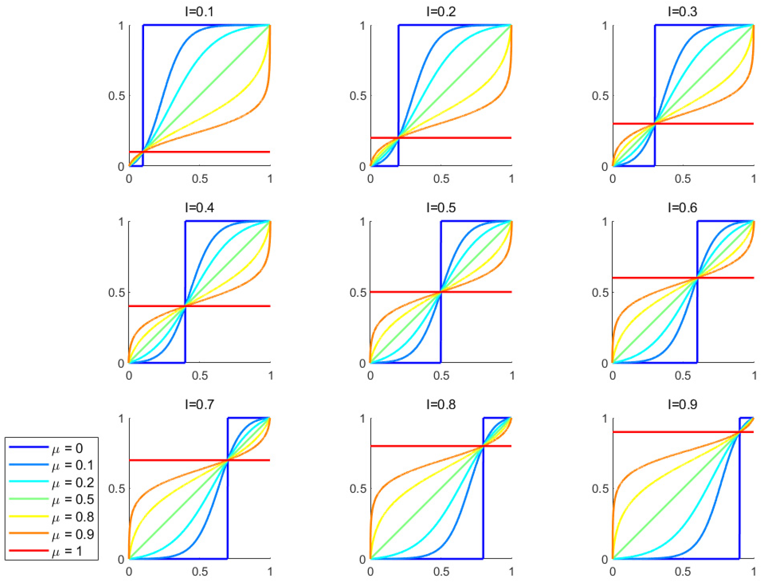
Figure 2.
CMG as input feature modulator for MLP. (A) Illustration of MLP where the features at input layer are modulated by CMG (B) Comparison of different schedulers’ learning rate decay (C) Evaluation results of different schedulers. In the legend, each trial’s accuracy (ACC) and area across the epochs (AAE) are shown. The accuracy of each trial is also shown beside the curve, and this is the same for D and E (D) Test accuracy curves of MLP modulated by CMG, linear (best-performance counterpart learnable function), and original MLP on CIFAR10 (E) Test accuracy curves of MLP modulated by CMG, linear (best-performance counterpart learnable function), and original MLP on CIFAR100.
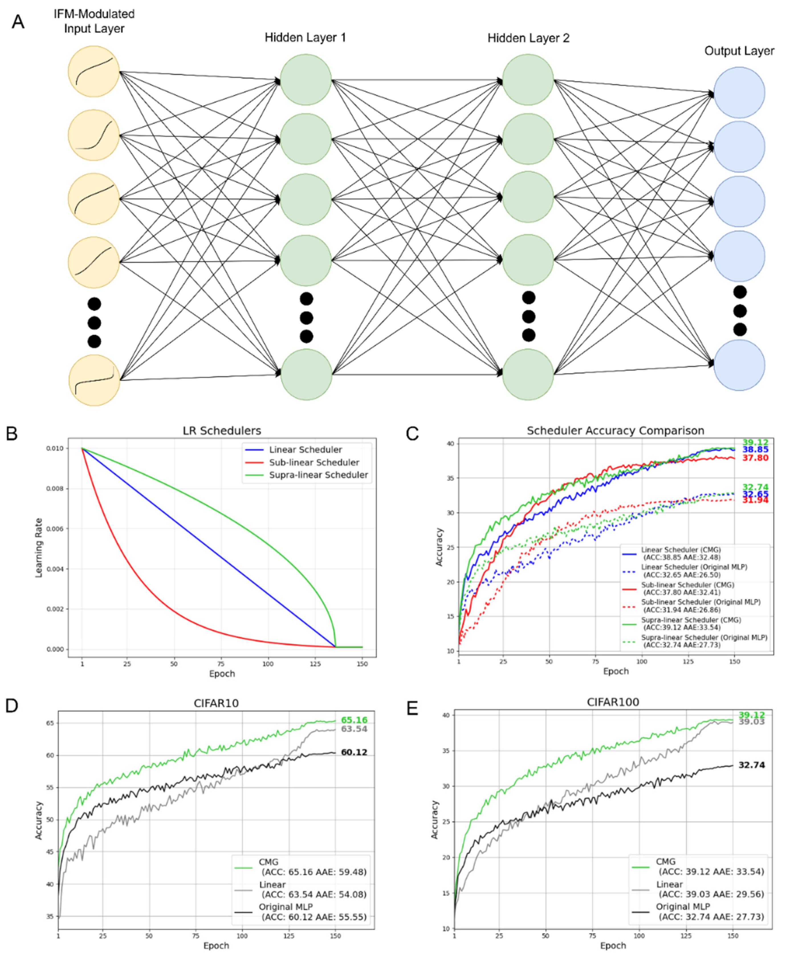
Figure 3.
Comparison between images before and after CMG modulation. (Leftmost) The original image in CIFAR10 test set (Middle) Image after CMG modulation (Right) Bar plot comparing the RMS contrast between original image and CMG-modulated image.
Figure 3.
Comparison between images before and after CMG modulation. (Leftmost) The original image in CIFAR10 test set (Middle) Image after CMG modulation (Right) Bar plot comparing the RMS contrast between original image and CMG-modulated image.
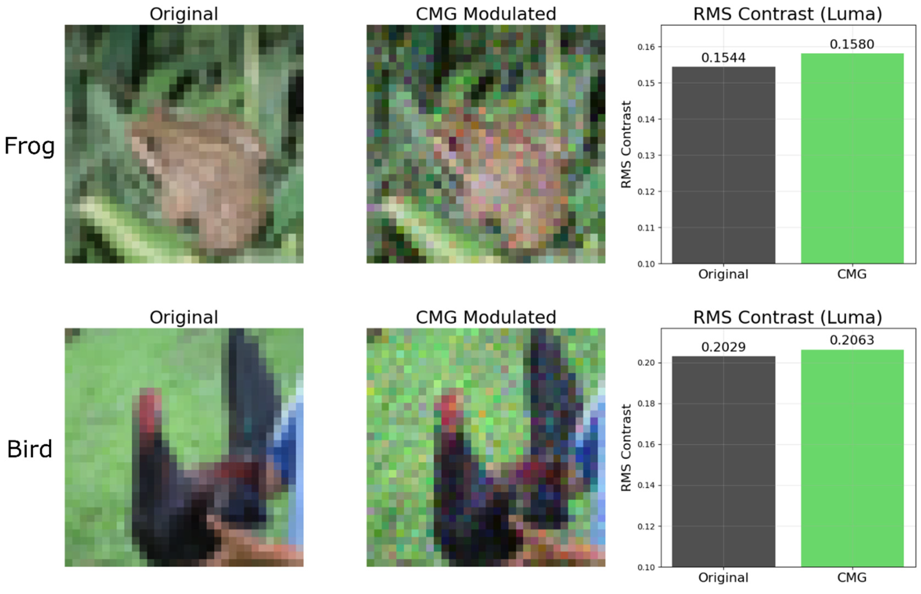
Figure 4.
CMG transformation improves EM image neuron segmentation algorithm. (A): The working pipeline of neuron segmentation experiment. Firstly, the 3D brain EM image volume is sent into a 3D U-Net[21] which predicts the affinity values (black arrows between smaller cubes) between neighboring voxels in the volume. Affinity values in the original affinity graph (middle left) are then transformed by CMG function for enhancement and the new values are indicated by blue arrows in the transformed affinity graph (middle right). Finally, the transformed affinity graphs are segmented using the pipeline proposed by Funke et al[11] to produce the predicted neuron segments (rightmost). (B): CREMI score (the lower the better) evaluation on CREMI training set B. Each line represents one inflection point (I) and x-axis shows the μ values. SOTA (black dot) and best CMG-enhanced (μ=0.4 and I = 0.3) are highlighted with black and green arrows respectively. (C): Bar plot comparing the CREMI score (the lower the better) between the best result obtained using CMG-enhanced (μ=0.4 and I = 0.3) and SOTA. (D): Segmentation quality comparison between CMG-enhanced, CREMI benchmark and SOTA.
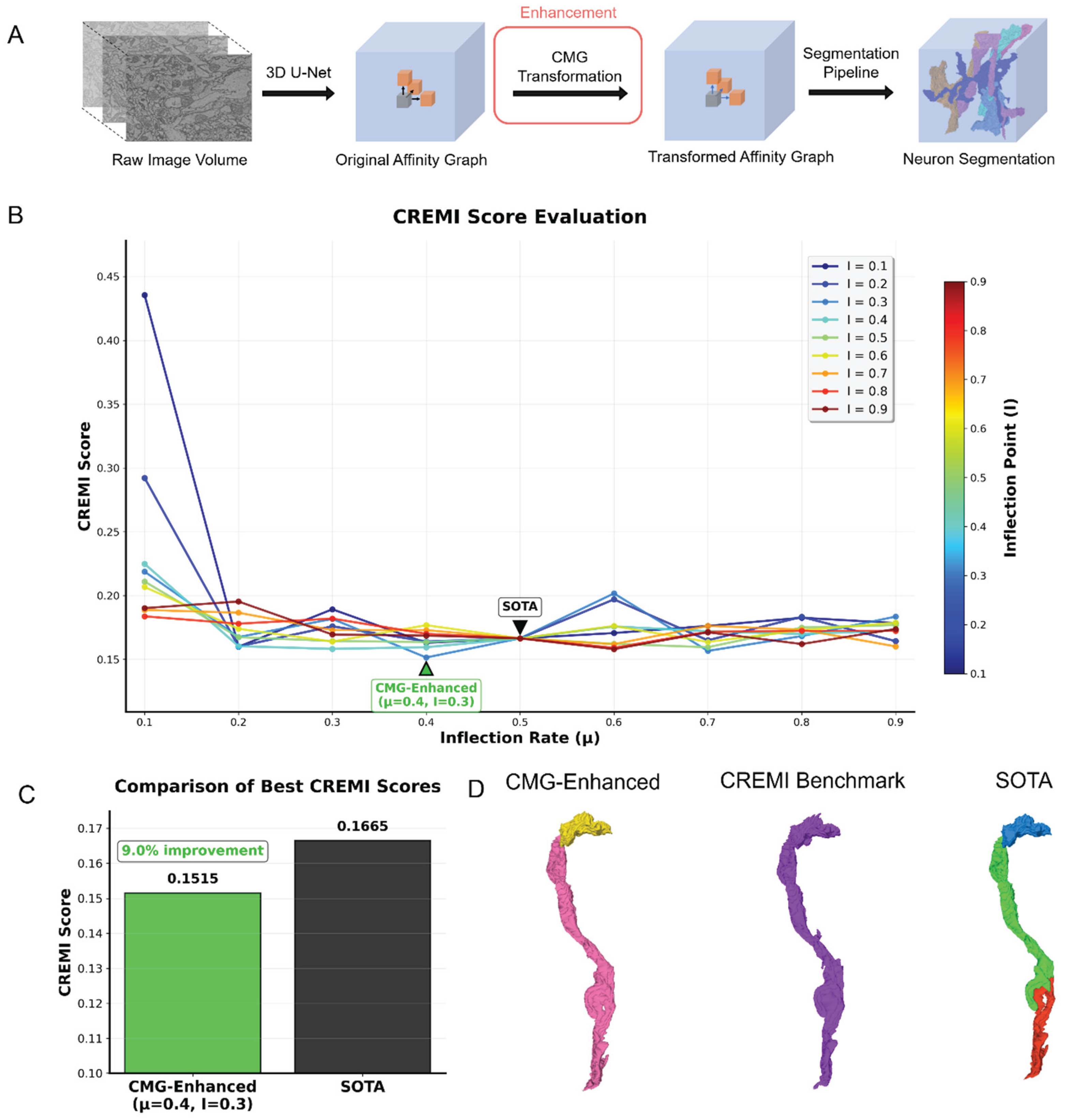

Table 1.
Grid-search space for neuron segmentation experiments.
| Inflection rates (μ) | 0.1 – 0.9 in increments of 0.1 |
| Deviate inflection points (I) | 0.1 – 0.9 in increments of 0.1 |
| Merge functions (MF) | {median_aff_histograms, 85_aff_histograms, median_aff, 85_aff, max_10} |
| Thresholds | 0.1 – 0.9 in increments of 0.1 |
Table 2.
Configuration of MLP training.
| Optimizer | SGD |
| Momentum | 0.9 |
| Weight decay | 5e-4 |
| Batch sizes | {32, 64, 128} |
| Initial learning rates | {0.025, 0.01, 0.001} |
| Dropout rate | 0.3 |
Disclaimer/Publisher’s Note: The statements, opinions and data contained in all publications are solely those of the individual author(s) and contributor(s) and not of MDPI and/or the editor(s). MDPI and/or the editor(s) disclaim responsibility for any injury to people or property resulting from any ideas, methods, instructions or products referred to in the content. |
© 2025 by the authors. Licensee MDPI, Basel, Switzerland. This article is an open access article distributed under the terms and conditions of the Creative Commons Attribution (CC BY) license (http://creativecommons.org/licenses/by/4.0/).
Copyright: This open access article is published under a Creative Commons CC BY 4.0 license, which permit the free download, distribution, and reuse, provided that the author and preprint are cited in any reuse.


