Effect of Dataset Partition and Normalization Methods in the Hyperparameters Optimization Phase on the Efficiency of The Levenberg-Marquardt Algorithm

1. Introduction

The emergence of digital technology and its own revolution has facilitated to boost the performance of many other sectors. Thus, man made the transition from manual work to full automation of many of his precarious tasks. This digital advance is the result of neural networks incorporated in a box for which an algorithm is preestablished for adapting to new circumstances.Indeed, artificial neural networks (ANNs) are mathematical models inspired by neurobiology that perform calculations similar to those of human intelligence. They have been widely investigated and applied these last years to classification, pattern recognition, regression, and forecasting problems [1,2,3].Multilayer perceptron neural networks (MLP) are one of the ANN variants the most commonand applied [4,5,6,7,8,9]. In a non-linear regression context for the purpose of empirical data forecasting, the explanatory and predictive performances of MLPs are generally affected by hyper-parameters (number of hidden layers, number of hidden nodes, set of transfer functions and learning rate), the learning algorithm, the partition rate of the data set and the input data normalization method [10,11,12,13,14,15,16,17] but also the sample size [18,19].The selection of the best configuration of these factors in the process of learning a dataset is a laborious task, which often requires a thorough knowledge of optimization methods. An inappropriate choice of these factors leads to problems among others: local minima, slow convergence or non-convergence, dependence on initial parameters and over-adjustment. However, the work of Tohoun [20] reveals that the use of Levenberg-Marquardt algorithm (LM) [18] compared to other more commonly used gives better predictive performance. Thus, there are some questions that are directly linked to the use of MPL models, although they are more applied. In this study,we will focus on the determination of optimal hyper-parameters with the LM algorithm based on the partition rate of a dataset, the input data normalization method and the sample size in a context of empirical data prediction .Specifically, we aim: (i) to identify optimal hyper-parameters and the minimum sample to train a MLP with LM algorithm based on dataset partition rates for each input data normalization method; (ii) to compare the quality of predictive performance of MLPs from optimal hyper-parameters and from appropriate partition rate of a dataset with the minimum sample size according to input data normalization methods.

2. Materials and Methods

2.1. Specification of Model

This section reproduces the approach adopted in [20] in process of evaluating the performance of different algorithms.

Let $x={\left(x_1,\dots ,x_p\right)}^{\top }\in {\mathbb{R}}^p$ be the vector of inputs, $w_i={\left(w_{i0},\dots ,w_{ip}\right)}^{\top }\in {\mathbb{R}}^{p+1}$ be a parameter vector for the hidden unit $i(1\le i\le m),m\in \mathbb{N}$ and $\beta ={\left({\beta }_0,\dots ,{\beta }_m\right)}^{\top }\in$${\mathbb{R}}^{m+1}$ be a parameter vector for the only output unit. Multilayer perceptron (MLP) function with m hidden units and one output unit can be written as follows:

$$F(\theta ,x)=g\left(\sum _{i=1}^m{\beta }_{i}f\left(\sum _{j=1}^p{w}_{ij}{x}_j+w_{i0}\right)+{\beta }_0\right)$$

(1)

where $\theta =\left(w_{10},\dots ,w_{m0};w_{11},\dots ,w_{1p};\dots ;w_{m1},\dots ,w_{mp};{\beta }_0;{\beta }_1,\dots ,{\beta }_m\right);g$ and f (real value functions) are output and hidden-unit activation functions respectively. Let ${\mathsf{\Theta }}_m\subset {\mathbb{R}}^{m(p+2)+1}$ be a compact (i.e. closed and bounded) subset of possible parameters of the regression model family $\mathcal{S}=\left\{F_{\theta }\left(x\right),\theta \in {\mathsf{\Theta }}_m,x\in {\mathbb{R}}^p\right\}$ with $Y=$$F_{\theta }\left(X\right)+ϵ$.

Let $D=\left\{\left(x_1,y_1\right),\dots ,\left(x_n,y_n\right)\right\}$ with n a strictly positive integer be the observed data coming from a true model ${\left(X_t,Y_t\right)}_{t\in \mathbb{N}}$ for which the true regression function is $F_{{\theta }^{\circ }}$, for an ${\theta }^0$ in the interior of ${\mathsf{\Theta }}_m$. Learning consists to estimate the true parameter ${\theta }^0$ from the observations D. This can be done by minimizing the mean square error function:

$$E\left(\theta \right)=\sum _{t=1}^n{\displaystyle \frac{1}{2}}{\left(y_t-F\left(\theta ,x_t\right)\right)}^2$$

(2)

with respect to parameter vector $\theta \in {\mathsf{\Theta }}_m$. Different algorithms are used and based on gradient descent procedure.

2.2. Simulation Plan

Let $\mathbf{X}ϵ{\mathbb{R}}^8$ be a vector of input variables and $\mathbf{Y}ϵ\mathbb{R}$, a univariate output variable.

We have $Y=\vartheta \left(X\right)+\in$ where $\vartheta :{\mathbb{R}}^8⟶\mathbb{R}$ and $ϵ\in \mathbb{R}$ is a vector of residual variables. To guarantee the nonlinearity of $\vartheta$ [17], we chose Log weibull-type non linear function [41] as such :

$$\vartheta (X_1,...,X_8)=\phi (X_1,X_2,X_3,X_5,X_8)+\omega (X_2,X_3,X_7)$$

(3)

where

$$\phi (X_5,X_6,X_7,X_8)={\alpha }_1{X}_7+{\alpha }_6{X}_6+{\displaystyle \frac{{\alpha }_5}{X_5}}+{\displaystyle \frac{{\alpha }_8}{X_8}}$$

(4)

and

$$\omega (X_2,X_3,X_4,X_7)=log\left(({\alpha }_3{X}_3+{\alpha }_2{x}_2)\right)\ast exp({\alpha }_1{x}_1+{\alpha }_4{x}_4)$$

(5)

The coefficient of the features X corresponding used in the simulation study was prespecified as in Table 1 :

Regarding features vector $X={(X_1,X_2,...,X_8)}^T$ , its components, respectively, follow normal, log-normal, binomial negative, Poisson, weibull, geometric, exponential and normal distribution laws. The next one table summary them with their distribution law and linked parameters. In additional take into account random part at $\vartheta \left(X\right)$ that means $ϵ$.

2.2.1. Generation of the data

In context of this study, a population of size N = 10000 was generated. Process is summaried into those following steps:

Step 1. Generate the input variables X1 to X8 and $ϵ$ from their respective distribution for $N=10.000$.

Step 2. Calculate $\vartheta \left(X\right)$ using (15) from values of coefficients ${\alpha }_1$ to ${\alpha }_7$ and generated input variables $X_1$ to $X_7$.

Step 3. Generate outcome variables $\mathbf{Y}$ for $N=10.000$, from each $ϵ$ distribution adds to $\vartheta \left(X\right)$.

Step 4. Use the boostraping technique to extract samples of different sizes:

$n_i=\{25;50;75;100;150;300;500\}$

2.2.2. Prepocessing of dataset

Before each implementation the starting sample is divided into 2: traning data and test data. Here different dataset partition rates will be used (65%, 70%, 75%, 80%, 85% for the training and 35%, 30%, 25%, 20%, 15% for the test). Moreover, different input data normalization methods will also be used (Min-Max Normalization; Z-Score Normalization; Decimal Scaling, median and unscaled normalization)

The characteristics considered for the model are as follows:

• Activations functions
  Four differents tranfers functions have been used at level of hidden layer and output layer as such : Log-sigmoid, exponential, Hyperbolic tangent, and identity functon as listed in previous section.
• Number of hidden neurons as introduce above, vary between
  $\{1,3,5,7,8,9,11,13,15,16,17\}$
• Learning rate r took value in interval ]0,1] especially,
  $r=\{0.15,0.25,0.35,0.45,0.55,0,65,0.75,0.85\}$
• And finally, LM algorithm is applied for learning.

2.2.3. Implementation of 3-MLP Model

The function ”mlp” of RSNNS package (Bergmeir and Benıtez, 2012) was used for the prediction. A 3−MLP model was used by varying partition rate, normalizations methods and hyper parameters for each sample size. With respect to hyper parameters, 16 combinations of activation functions (AF) were used: four differentes function (TanH, Exponentiel, Logistic and Linear ) have been applyed at hidden layer and four other at output (TanH, Exponentiel, Logistic and Linear ). In additional, 9 different numbers of node in the hidden layer were considered.A total of 500 replications was performed on each sample size to the analyze performance of the method. Initial weights were generated randomly according to the uniform law in the range −3 and 3. The stopping criteria used are the combination of a fixed number of epochs, NE= 1000 and a sufficiently small training error less than or equal to ${10}^{-6}$.

2.2.4. Performance criteria

Then to evaluate the performance of the network, at each sample size $n_i$, the previous step is repeated 500 times, that means after gathering set of parameters and fed to the corresponding algorithm, the last one have to iterate 500 times. Thereby, the average values of the performance criteria are calculated.

In this section we consider $F_{{\theta }_i},\overline{F_{{\theta }_i}},y_i \mathrm{and} \overline{y}$ respectively as desired obsersed from MLP model, mean of desired obsersed from MLP model, target value observed from simulated dataset and mean of target value observed from simulated dataset

$$\begin{array}{cc}\hfill R^2=& 1-{\displaystyle \frac{{\sum }_{i=1}^n{\left(y_i-F_{{\theta }_i}\right)}^2}{{\sum }_{i=1}^n{\left(y_i-\overline{y}\right)}^2}}\hfill \end{array}$$

(6)

The mean absolute percentage error (MAPE) is the mean or average of the absolute percentage errors of forecasts. Error is defined as actual or observed value minus the forecasted value. The smaller the MAPE the better the forecast.

$$MAPE={\displaystyle \frac{1}{n}}\sum _{i=1}^n{\displaystyle \frac{\left|F_{{\theta }_i}-y_i\right|}{y_i}}$$

(7)

The coefficient of determination ($R^2$) inform about the accuracy of the network with an $R^2$ closed to "1" indicates good performance (Shahin et al., 2008).

Coefficient of determination (CV), also known as relative standard deviation, coefficient of variation is a statistical concept that accounts for relative variability in data sets. Specifically, it indicates the size of a standard deviation to its mean.

$$CV={\displaystyle \frac{\sigma }{\overline{x}}}\times 100$$

(8)

2.3. Statistical comparisons methods

The results got from simulation design in context of study are assessed due to ANOVA (analysis of variance) and LSD.test for multiple comparaison means; especially applied on those factors which affect the performances of the MLP. Those analysis have been run on output of simulation ($R^2$ and MAPE) for each normalization method, sample size and percentage of train and test. Boxplot too was used to present significant interaction between hyper parameters of the network according to the partition rate, normalization method and sample size.

3. Mains Results

From simulation results, a total number of 295680 multilayer perceptron network model have been built. Either dataset of 4435200 rows with seven features and three targets variables (three performances criteria).

3.1. Analysis of Hyper-Parameters’ Effect on the 3−MPL Performance According to Partition Rate and Normalization Methods

The following section outlines the performance of normalization methods such as non-normalization, decimal, median and z-score methods.

3.1.1. Hyperparameter’s Effect on 3-MLP Peformance According Unscaled (Non Normalization) Method

Hyper-parameters’ effect on the 3 − MPL performance criteria ($R^2$ and MAPE) shows same trends. Third and fourth order-interaction effects between number of nodes (N), learning rate (LR), sample size (S), activation functions on $R^2$ and MAPE are not significant at 5% level for all partition rate. However, the interaction effect of individual factors and first-order interaction (1) varies from one partition rate to another except for the interaction between learning rate (L), sample size (S) and node (N) as well as the interaction between learning rate and activation functions (AF) which are shown to be significant from one partition to another. The following table shows the level of significance of the interactions at at 1‰and at 5% threshold.

Table 3. Effect of hyper-parameters on 3−MLP performance: p-values from ANOVA

		Partition rate (%)
H-parameter	df	65-35		70-30		75-25		80-20		85-15
		$R^2$	MAPE	$R^2$	MAPE	$R^2$	MAPE	$R^2$	MAPE	$R^2$	MAPE
S	6	0.001	0.07	0.001	0.68	0.001	0.08	0.001	0.51	0.001	0.10
N	10	0.08	0.70	0.001	0.67	0.55	0.001	0.001	0.001	0.46	0.55
LR	7	0.19	0.19	0.64	0.23	0.17	0.03	0.41	0.54	0.68	0.51
AF	16	0.001	0.12	0.001	0.07	0.001	0.001	0.001	0.28	0.001	0.46
L:AF	127	0.001	0.001	0.001	0.001	0.001	0.001	0.001	0.25	0.001	0.02
S :N	76	0.99	0.78	0.001	0.54	0.03	0.01	0.14	0.001	0.88	0.64
S :AF	27	0.001	0.001	0.001	0.36	0.001	0.01	0.001	0.86	0.001	0.001
LR :S	35	0.67	0.67	0.08	0.66	0.01	0.001	0.16	0.55	0.01	0.61
LR :N	70	0.74	0.74	0.28	0.71	0.03	0.001	0.73	0.001	0.90	0.50
N :AF	175	0.15	1.00	0.09	1	0.02	0.98	0.04	0.99	0.46	1
S :N:AF	307	0.59	0.001	0.01	0.001	0.95	0.33	0.34	0.99	0.32	0.001
S:N:LR	520	0.001	0.03	0.001	0.01	0.001	0.001	0.001	0.001	0.001	0.1

Table 3. Effect of hyper-parameters on 3−MLP performance: p-values from ANOVA

		Partition rate (%)
H-parameter	df	65-35		70-30		75-25		80-20		85-15
		$R^2$	MAPE	$R^2$	MAPE	$R^2$	MAPE	$R^2$	MAPE	$R^2$	MAPE
S	6	0.001	0.07	0.001	0.68	0.001	0.08	0.001	0.51	0.001	0.10
N	10	0.08	0.70	0.001	0.67	0.55	0.001	0.001	0.001	0.46	0.55
LR	7	0.19	0.19	0.64	0.23	0.17	0.03	0.41	0.54	0.68	0.51
AF	16	0.001	0.12	0.001	0.07	0.001	0.001	0.001	0.28	0.001	0.46
L:AF	127	0.001	0.001	0.001	0.001	0.001	0.001	0.001	0.25	0.001	0.02
S :N	76	0.99	0.78	0.001	0.54	0.03	0.01	0.14	0.001	0.88	0.64
S :AF	27	0.001	0.001	0.001	0.36	0.001	0.01	0.001	0.86	0.001	0.001
LR :S	35	0.67	0.67	0.08	0.66	0.01	0.001	0.16	0.55	0.01	0.61
LR :N	70	0.74	0.74	0.28	0.71	0.03	0.001	0.73	0.001	0.90	0.50
N :AF	175	0.15	1.00	0.09	1	0.02	0.98	0.04	0.99	0.46	1
S :N:AF	307	0.59	0.001	0.01	0.001	0.95	0.33	0.34	0.99	0.32	0.001
S:N:LR	520	0.001	0.03	0.001	0.01	0.001	0.001	0.001	0.001	0.001	0.1

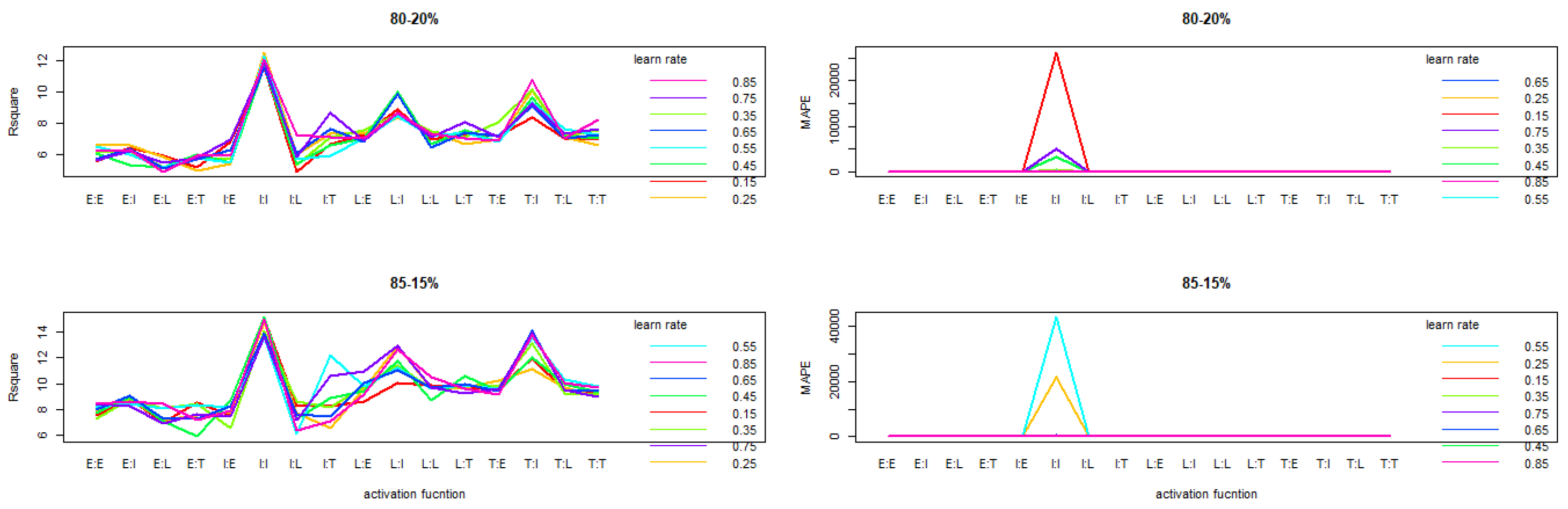
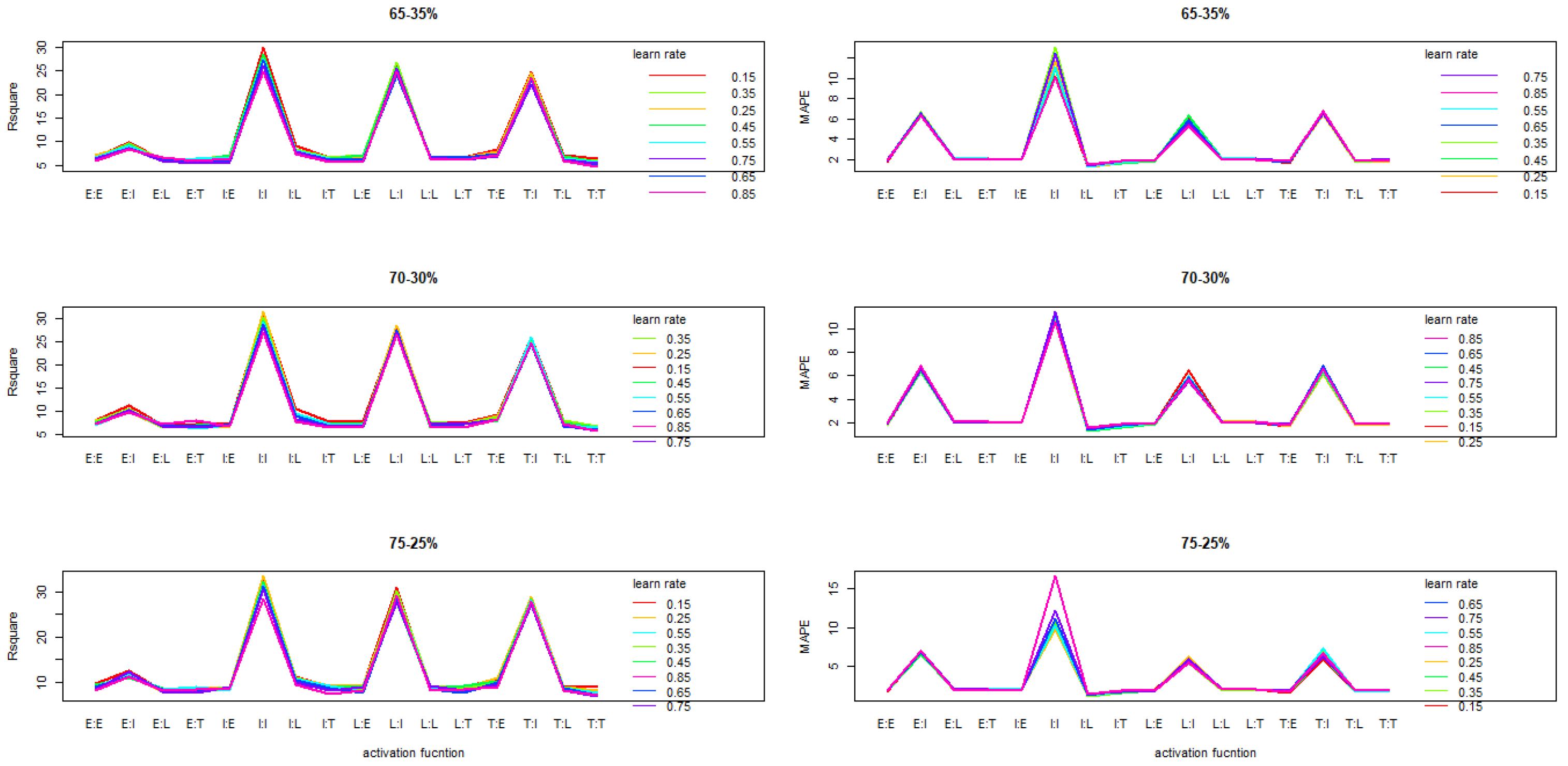
Interaction plot related to activation function and learning rate on $R^2$ and MAPE reveals that the trend are similar from one partition rate to another.We note however an increase of the $R^2$ when the rate allocated for training increases. The interaction plot also shows that activation function Tanh and Identity (TI), Logistic and Identity (LI) performed better on 3-MLP for all learning rates (Figure 1) when applying this method for normalization.

However, the interaction effect between node, learn rate and sample size by applying multiple comparisons of treatments by means of LSD and a grouping of treatments showed a difference in performance related to hyperparameters combinations. This process has allowed the optimal selection of those combinations according to the number of nodes and the minimum sample size with respect the $R^2$ and MAPE. We note moreover, as elaborated by the table, that the optimal sample size for the 3-MLP configuration is $n_i=25$ from one number of node to another.

Table 4. Interaction effect of S:L:N on 3-MLP performance acording to $R^2$ and MAPE from LSD.

node	learn rate	sample size	${\mathit{R}}^2$	MAPE
1	0.65	25	18.43	6.21
3	0.35	25	21.11	7.18
5	0.35	25	19.24	4.74
7	0.35	25	20.24	5.95
9	0.55	25	18.01	6.25
11	0.75	25	17.99	5.95
13	0.65	25	16.44	4.23
15	0.55	25	18.68	2.75
17	0.35	25	20.37	2.59

Table 4. Interaction effect of S:L:N on 3-MLP performance acording to $R^2$ and MAPE from LSD.

node	learn rate	sample size	${\mathit{R}}^2$	MAPE
1	0.65	25	18.43	6.21
3	0.35	25	21.11	7.18
5	0.35	25	19.24	4.74
7	0.35	25	20.24	5.95
9	0.55	25	18.01	6.25
11	0.75	25	17.99	5.95
13	0.65	25	16.44	4.23
15	0.55	25	18.68	2.75
17	0.35	25	20.37	2.59

The relative performance of the hyperparameters on the 3-MLP model showed that the use of the hyperbolic as activation function with a partition rate of 75% for training and 25% for testing with a number of nodes equal to 13 at the hidden layer and a learning rate of 0.75 led to the best 3-MLP model performance. The next table illustrates the relative performances.

Table 5. Effect of hyper-parameters on 3−MLP performance according to minimal sample size and unnorm method.

AF	node	L	S	Partition rate (%)
				65-35		70-30		75-25		80-20		85-15
				$R^2$	MAPE	$R^2$	MAPE	$R^2$	MAPE	$R^2$	MAPE	$R^2$	MAPE
TI	1	0.35	25	16.89	6.64	7.12	7.33	6.37	6.99	5.82	9.00	0.85	7.23
LI	3	0.35	25	2.68	9.71	7.97	15.01	2.92	7.91	2.76	21.04	19.64	14.62
LI	5	0.35	25	4.53	9.38	4.68	10.31	15.50	7.87	24.91	8.76	13.89	9.50
TI	7	0.65	25	13.70	12.10	13.77	9.14	13.23	7.79	16.02	15.14	35.25	11.08
TI	9	0.75	25	12.02	6.78	12.25	5.46	15.26	8.67	8.67	7.54	32.48	5.15
TI	11	0.55	25	9.21	9.07	16.58	6.63	13.56	11.75	14.85	10.97	35.72	5.71
TI	13	0.75	25	12.75	11.14	17.94	8.14	28.15	9.40	18.66	15.16	37.96	7.52
TI	15	0.55	25	12.68	7.06	12.40	9.26	17.80	10.53	20.65	9.53	47.85	10.55
TI	17	0.75	25	13.73	5.48	10.78	7.61	14.28	8.33	19.11	19.46	32.21	6.09

AF: Activation function, Node: number of unit at hidden layer, L: Learning rate, S: Sample size.

Table 5. Effect of hyper-parameters on 3−MLP performance according to minimal sample size and unnorm method.

AF	node	L	S	Partition rate (%)
				65-35		70-30		75-25		80-20		85-15
				$R^2$	MAPE	$R^2$	MAPE	$R^2$	MAPE	$R^2$	MAPE	$R^2$	MAPE
TI	1	0.35	25	16.89	6.64	7.12	7.33	6.37	6.99	5.82	9.00	0.85	7.23
LI	3	0.35	25	2.68	9.71	7.97	15.01	2.92	7.91	2.76	21.04	19.64	14.62
LI	5	0.35	25	4.53	9.38	4.68	10.31	15.50	7.87	24.91	8.76	13.89	9.50
TI	7	0.65	25	13.70	12.10	13.77	9.14	13.23	7.79	16.02	15.14	35.25	11.08
TI	9	0.75	25	12.02	6.78	12.25	5.46	15.26	8.67	8.67	7.54	32.48	5.15
TI	11	0.55	25	9.21	9.07	16.58	6.63	13.56	11.75	14.85	10.97	35.72	5.71
TI	13	0.75	25	12.75	11.14	17.94	8.14	28.15	9.40	18.66	15.16	37.96	7.52
TI	15	0.55	25	12.68	7.06	12.40	9.26	17.80	10.53	20.65	9.53	47.85	10.55
TI	17	0.75	25	13.73	5.48	10.78	7.61	14.28	8.33	19.11	19.46	32.21	6.09

AF: Activation function, Node: number of unit at hidden layer, L: Learning rate, S: Sample size.

3.1.2. Hyperparameter’s Effect on 3-MLP Peformance According to Decimal Method

Hyper-parameters’ effect on the 3 − MPL performance criteria ($R^2$ and MAPE) shows different trend from one partition to another and from order of interaction. . Third and fourth order-interaction effects between number of nodes (N), learning rate (LR), sample size (S), activation functions on $R^2$ and MAPE are not significant at 5% level for all partition rate. However, the first and second order interaction effect is noted between the leanring rate (L) and the activation function (AF) and between the sample size (S), the number of nodes (N) and the learning rate. The table below shows the significance level at the 5% and 1% threshold.

Table 6. Effect of hyper-parameters on 3−MLP performance according to decimal method : p-values from ANOVA.

H-parameter	df	Partition rate (%)
		65-35		70-30		75-25		80-20		85-15
		$R^2$	MAPE	$R^2$	MAPE	$R^2$	MAPE	$R^2$	MAPE	$R^2$	MAPE
AF	15	0.33	0.001	0.33	0.001	0.81	0.001	0.20	0.001	0.18	0.001
N	16	0.85	0.82	0.74	0.36	0.43	0.57	0.92	0.41	0.02	0.16
L	7	0.54	0.001	0.55	0.001	0.53	0.001	0.72	0.001	0.70	0.001
S	6	0.001	0.57	0.001	0.001	0.001	0.36	0.001	0.001	0.001	0.14
N:AF	143	0.001	0.04	0.24	0.15	0.03	0.08	0.65	0.25	0.42	0.01
L:AF	127	0.02	0.01	0.001	0.001	0.01	0.001	0.04	0.03	0.49	0.001
L:S	55	0.001	0.58	0.77	0.95	0.04	0.63	0.89	0.26	0.09	0.33
L:N	55	0.980	0.96	0.45	0.54	0.78	0.01	1		0.001	0.84
S:N	62	0.83	0.40	0.98	0.38	1	0.17	0.97	0.50	0.01	0.33
S:AF	143	0.28	0.60	0.001	0.001	0.77	0.13	0.83	0.34	0.89	0.001
S:N:AF	1007	0.25	0.15	0.05	0.22	0.48	0.001	0.35	0.001	0.25	0.56
L:S:N	504	0.001	0.001	0.001	0.001	0.001	0.001	0.001	0.001	0.001	0.47

Table 6. Effect of hyper-parameters on 3−MLP performance according to decimal method : p-values from ANOVA.

H-parameter	df	Partition rate (%)
		65-35		70-30		75-25		80-20		85-15
		$R^2$	MAPE	$R^2$	MAPE	$R^2$	MAPE	$R^2$	MAPE	$R^2$	MAPE
AF	15	0.33	0.001	0.33	0.001	0.81	0.001	0.20	0.001	0.18	0.001
N	16	0.85	0.82	0.74	0.36	0.43	0.57	0.92	0.41	0.02	0.16
L	7	0.54	0.001	0.55	0.001	0.53	0.001	0.72	0.001	0.70	0.001
S	6	0.001	0.57	0.001	0.001	0.001	0.36	0.001	0.001	0.001	0.14
N:AF	143	0.001	0.04	0.24	0.15	0.03	0.08	0.65	0.25	0.42	0.01
L:AF	127	0.02	0.01	0.001	0.001	0.01	0.001	0.04	0.03	0.49	0.001
L:S	55	0.001	0.58	0.77	0.95	0.04	0.63	0.89	0.26	0.09	0.33
L:N	55	0.980	0.96	0.45	0.54	0.78	0.01	1		0.001	0.84
S:N	62	0.83	0.40	0.98	0.38	1	0.17	0.97	0.50	0.01	0.33
S:AF	143	0.28	0.60	0.001	0.001	0.77	0.13	0.83	0.34	0.89	0.001
S:N:AF	1007	0.25	0.15	0.05	0.22	0.48	0.001	0.35	0.001	0.25	0.56
L:S:N	504	0.001	0.001	0.001	0.001	0.001	0.001	0.001	0.001	0.001	0.47

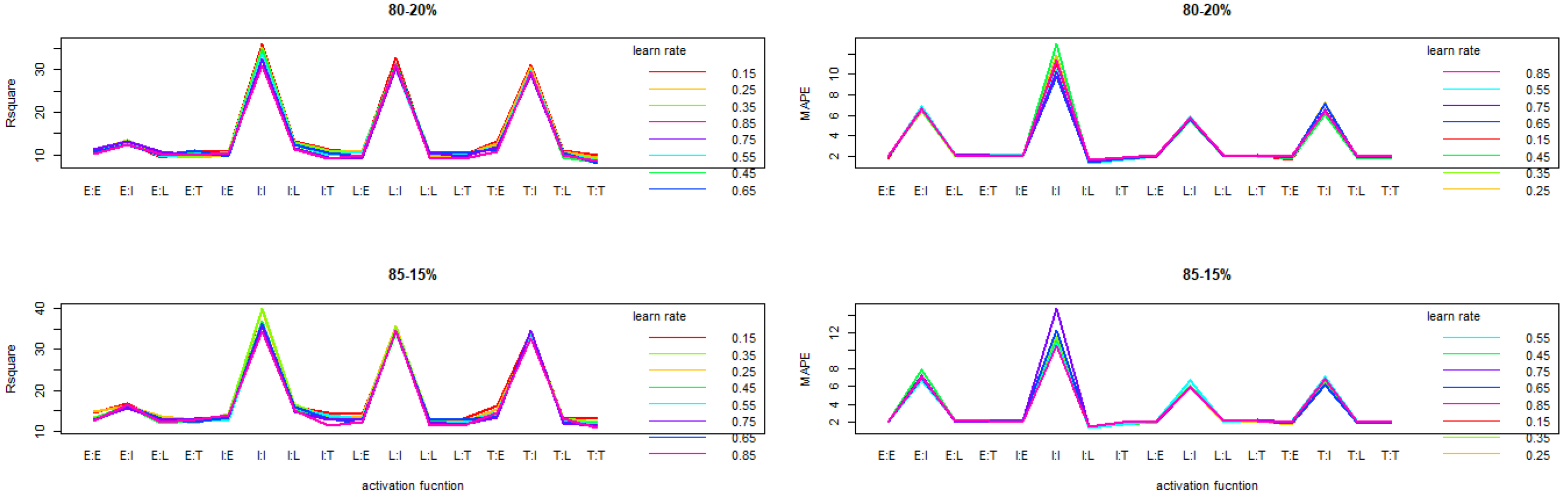
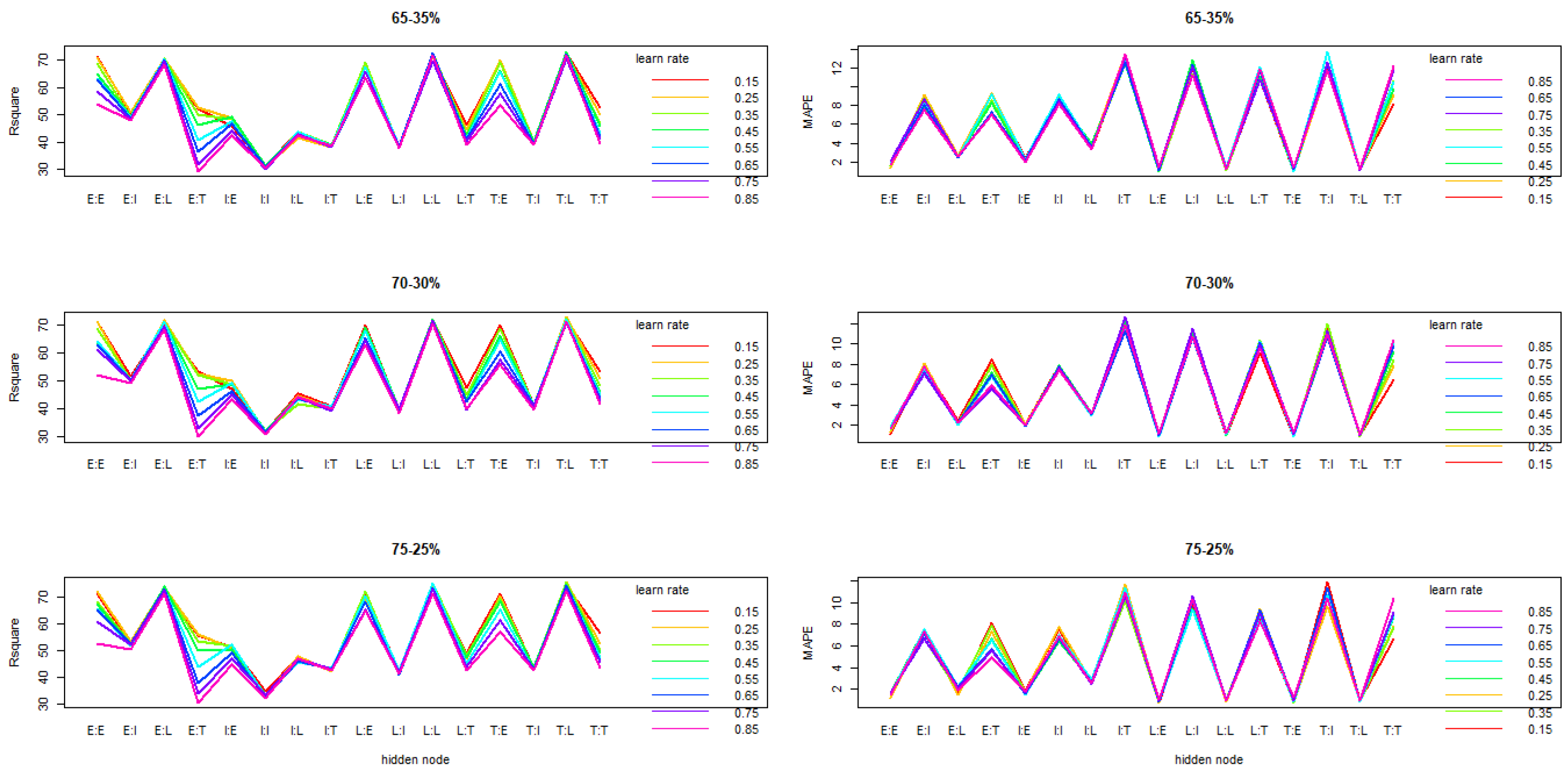
The tendency revealed by the interaction between the activation function and the learning rate is that of an oscillation. However, we note a regular performance of the exponential activation function (EE) and the linear one (II).From one partition rate to the other the trend is similar (Figure 2)

The application of decimal for data normalization showed that the second order interaction between N, L and S in function of the node and the optimal learning rate, 25, 50 and 75 are the minimum sample sizes according to $R^2$ and MAPE. See Table 7.

The performance related to the hyperparameters on the 3-MLP model showed that the use of the linear activation function with a partition rate of 85% for training and 15% for testing with a number of nodes equal to 3 in the hidden layer, for a learning rate equal to 0.35 with a sample size $n_i=25$ led to the best performance of the model. The Table 8 hereby illustrates the relative performance.

3.1.3. Hyperparameter’s Effect on 3-MLP Peformance According to Median Method

Hyper-parameters’ effect on the 3 − MPL performance criteria ($R^2$ and MAPE) shows that the second and third order-interaction effects between number of nodes (N), learning rate (LR), sample size (S), activation functions on $R^2$ and MAPE are not significant at 5% level for all partition rate. However, the first and second order interaction effect mainly between the leanring rate (L) and the activation function (AF) and between the sample size (S), the number of nodes (N) and the learning rate is noted. The Table 9 below shows the significance level at the 5% and 1% threshold.

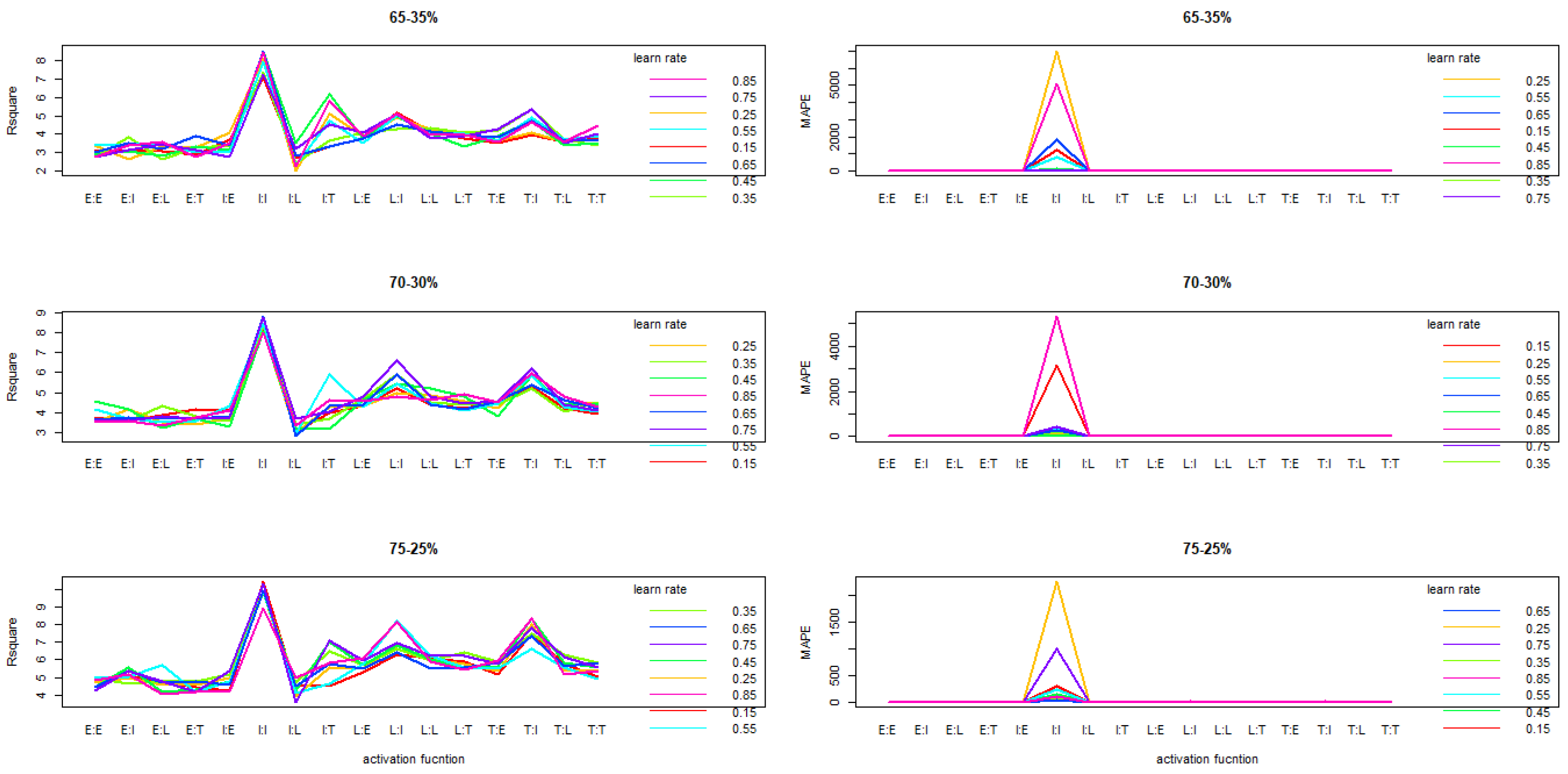
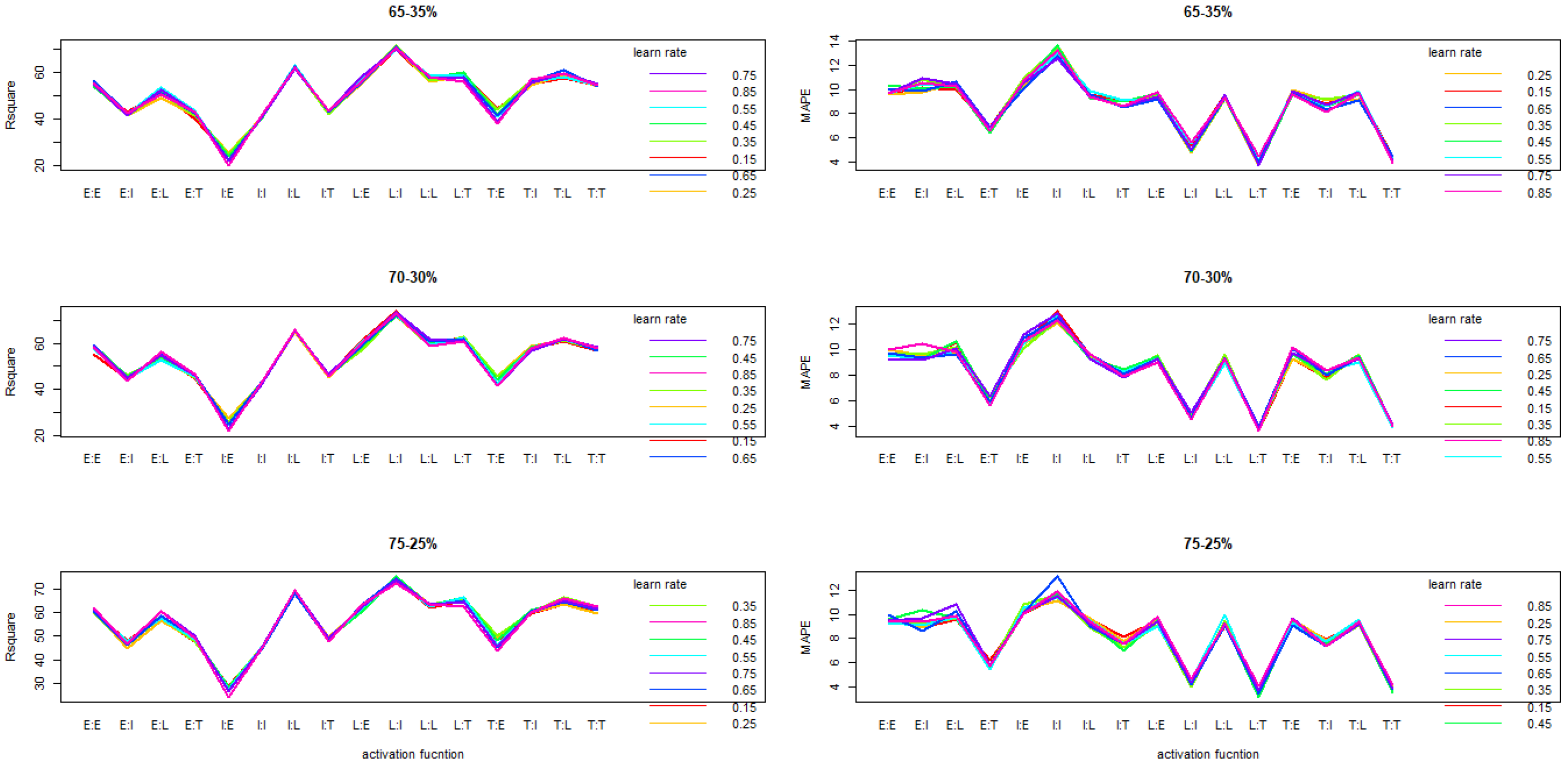
The application of the median for data normalization shows a relatively identical performance trend considering partition rate under the AF and L interaction .Interaction has shown that 3-MLP model likely perform better with logistic linear (LI) or hyperbolic linear (LI) compare to other actvations functions (Figure 3).

The second order interaction effect between N, L and S according to node and the appropriate learning rate, showed that the minimum sample size for the optimal hyperparameter configuration is equal to $n_i=25$ according to $R^2$ and MAPE. Table 10 displays their relative performances.

3.1.4. Hyperparameter’s Effect on 3-MLP Peformance According to Median Method

The relative performance of the hyperparameters on the 3-MLP model showed that the use of the hyperbolic activation function with a partition rate of 85% for training and 15% for testing with a number of nodes equal to 13 in the hidden layer, for a learning rate equal to 0.35 with a sample size of $n_i=25$ led to the best performance of the model. The Table 8 illustrates the relative performances.

Table 11. Effect of hyper-parameters on 3−MLP performance according to minimal sample size and decimal method.

AF	node	L	S	Partition rate (%)
				65-35		70-30		75-25		80-20		85-15
				$R^2$	MAPE	$R^2$	MAPE	$R^2$	MAPE	$R^2$	MAPE	$R^2$	MAPE
TI	1	0.65	25	25.48	4.35	25.12	6.00	27.63	5.32	27.16	15.26	71.29	3.07
TI	3	0.45	25	23.76	6.81	42.68	7.63	43.86	5.58	33.80	4.10	63.63	13.03
TI	5	0.15	25	35.57	4.99	38.45	3.63	26.72	5.06	46.79	5.87	58.21	7.24
LI	7	0.65	25	22.82	7.99	34.96	2.73	26.75	4.81	58.63	2.76	55.20	8.62
TI	9	0.25	25	21.92	5.47	20.49	6.12	41.72	6.21	34.24	13.99	53.27	3.62
LI	11	0.25	25	28.91	7.75	44.65	6.47	38.68	9.58	33.38	2.63	62.39	3.84
TI	13	0.35	25	24.22	7.58	26.73	5.46	42.27	10.81	42.93	16.89	67.88	4.43
LI	15	0.25	25	59.91	4.24	43.66	6.15	36.81	7.38	35.31	3.43	25.21	6.70
LI	17	0.15	25	61.02	3.91	42.39	4.80	40.49	7.38	36.07	9.42	31.91	9.48

Table 11. Effect of hyper-parameters on 3−MLP performance according to minimal sample size and decimal method.

AF	node	L	S	Partition rate (%)
				65-35		70-30		75-25		80-20		85-15
				$R^2$	MAPE	$R^2$	MAPE	$R^2$	MAPE	$R^2$	MAPE	$R^2$	MAPE
TI	1	0.65	25	25.48	4.35	25.12	6.00	27.63	5.32	27.16	15.26	71.29	3.07
TI	3	0.45	25	23.76	6.81	42.68	7.63	43.86	5.58	33.80	4.10	63.63	13.03
TI	5	0.15	25	35.57	4.99	38.45	3.63	26.72	5.06	46.79	5.87	58.21	7.24
LI	7	0.65	25	22.82	7.99	34.96	2.73	26.75	4.81	58.63	2.76	55.20	8.62
TI	9	0.25	25	21.92	5.47	20.49	6.12	41.72	6.21	34.24	13.99	53.27	3.62
LI	11	0.25	25	28.91	7.75	44.65	6.47	38.68	9.58	33.38	2.63	62.39	3.84
TI	13	0.35	25	24.22	7.58	26.73	5.46	42.27	10.81	42.93	16.89	67.88	4.43
LI	15	0.25	25	59.91	4.24	43.66	6.15	36.81	7.38	35.31	3.43	25.21	6.70
LI	17	0.15	25	61.02	3.91	42.39	4.80	40.49	7.38	36.07	9.42	31.91	9.48

3.1.5. Performance of Minmax Normalization Method on 3-MLP

Hyper-parameters’ effect on the 3 − MPL performance criteria ($R^2$ and MAPE) shows tendency of significant difference between them. In contrast to the previous normalization methods, the individual effects are significant except for the learning rate. Furthermore, the first and second order interaction between learning rate and activation function and between learning rate, node and sample size are significant. The following Table 12 shows the level of significance of the interactions at 1‰and at 5% threshold.

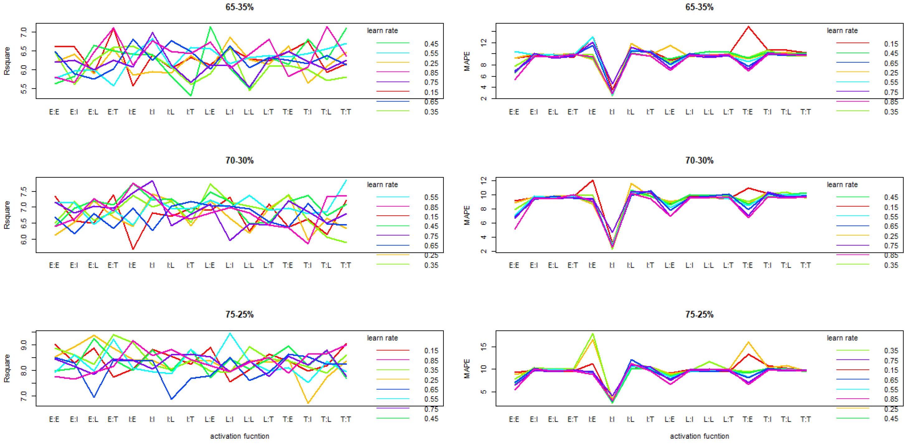
The trend illustrated by the interaction graphs between the activation functions and the learning rates over partitions rates is that of perfect similarity as indistinguishable dice at touch. High performance are reccorded for learning rate in range of [0.15; 0.45]. Activations functions as such LE, LL, LT, TE, TL, TT functions expressed highest performance compared to other. The Figure 4 shows their performance considering $R^2$ and MAPE.

Implementing minmax for data normalization showed that the second-order interaction between N, L, and S according to the number of nodes at the hidden layer and the optimal learning rate, resulted in minimum sample sizes such as 50, 75, 100 for the selection of optimal hyperparameters based on multiple comparisons of treatments using LSD and a clustering of treatments on $R^2$ and MAPE . The Table 13 displays the relative performances.

The relative performance of the hyperparameters on the 3-MLP model showed that at a partition rate of 85% for learning and 15% for testing with the logistic activation function (LL) or the hyperbolic logistic function (TL) with respectively a number of nodes equal to 9 and 11 in the hidden layer, for a learning rate equal to 0.15 and 0.25 with a sample size $n_i=100$ led to a better performance of the 3-MLP model. Applying these hyperparameters separately with this sample size led to relatively close performance in terms of R² and MAPE. The Table 14 illustrates the relative performances.

3.1.6. Performance of z-Score Normalization Method on 3-MLP

Hyper-parameters’ effect on the 3 − MPL performance criteria ($R^2$ and MAPE) shows interactions are significant according to partition rate. Especially, individual effects are significant except for the learning rate. Furthermore, the first and second order interaction between learning rate and activation function and between learning rate, node and sample size are significant. The following Table 15 shows the level of significance of the interactions at 1‰and at 5% threshold.

The use of z-score in the process of reducing the data to the same scale and to a relatively smaller value, has probably proved high performance performance of the 3-MLP regarding $R^2$ and MAPE when using a learning rate in the range [0.15, 0.45] with activation functions such as LI, LT and TT. This trend as shown in Figure 5 performance is similar from one partition rate to another.

The z-score method for data normalization considering the second order interaction between N, L and S according to the node at hidden layer and the appropriate learning rate, showed that 50, 75, 100 are the minimum sample sizes according to $R^2$ and MAPE for which optimal hyperparameters would be obtained for the 3-MLP setup. The Table 16 shows the relative performances of these hyperparameters.

The performance of hyperparameters on the 3-MLP model showed that at the 80%-20% or 85%-15% partition rate used for training and testing respectively, the model performed better with respect to R² and MAPE. The logistic-linear (LI) or logistic-hyperbolic (LT) activation functions have given better results. Better performance is obtained for nodes equal to 3, 5 or 15 at the hidden layer for learning rates equal to 0.15 or 0.25 with a sample size of $n_i=100$ as elaborated in Table 17.

3.2. Relative Performance of 3-MLP According to Normalization Methods and Partition Rate

The performance of the 3-MLP model considering hyperparameters reveals that all normalization methods outperformed at the partition rate 85% versus 15% for training and testing respectively. From one partition method to another, the unscaled ors without normalization method underperformed compared to the other methods. However, the minmax and z-score normalization methods perform better at each partition rate with better performance at 85%vs25%. Those performances are recorded with a minimum sample size $n_i=100$. The logistic (LL) and hyperbolic-logistic (TL) activation functions with the number of nodes in the hidden layer equal to 9 vs 11 and the learning rate equal to 0.15 vs 0.25 respectively led to the best performance of 3-MLP with respect to the perofmance criteria . Meanwhile, with the LT activation function using the z-score normalization method with a learning rate of about 0.25 and with 5 nodes in the hidden layer, the 3-MLP model performs somewhat similarly to the two previous configurations (Table 18).

4. Discussion

The assessment of hyperpameters in the construction of a 3-MLP model with the Levenberg Marquardt algorithm showed that z-score and minmax normalization methods give a different reading of the neural network models performance. Z-score is the better when the objective consist of assessing variability of the model while minmax leads to the construction of a model leading to approximate more the characteristics of the data derived from an environment. However, we observed that there is a relatively small difference in performance between them. This could be justified by the fact that these methods have partly in common an interval [0.1] on which they limit the original values (raws observations) according to [21,22]. This performance of z-score is due to the fact, according to [23]based on his study, the capability of z-score to transform data and maintains integrity of separate samples from different experiments and laboratories without remarkable loss of information content because of its skill to provide a way of standardising data across a wide range.

With respect to the minimum sample size ($n_i=100$) for training 3-MLP models, is not far off the one found by [20], i.e. a minimum value of 100 versus 150. This sample size (100) on which [24] has assessed methods of dataset scaling has obtained hightlight result. However, results that have been found out compare to those of [20] have shown a difference about type of model architecture developed, i.e. the number of nodes at the hidden layer is 9 versus 6. This difference could be explained by the resampling technique or the number of repetitions performed and on which each model expressed its performance.About total number of node at hidden layer sinks a lot of anchor : the determination of formulas for calculating the number of nodes in the hidden layer, which is a function of the number of nodes in the input[25,26].According to [27] the size of the hidden layer neurons is between the input layer size and the output layer size.If this is insufficient then number of output layer neurons can be added later on [25,26]. However, despite a number of those principles for determining suitable node at hidden layer, none is universally accepted in context of estimating the optimal number of hidden layer nodes[28]. In the limit, one could rely on heuristics to compute a number that can be used as a starting point for a search towards the optimum number of hidden layer nodes [29].

With regard to partition dataset, according to [28], the use of too few training samples in neural networks is not favourable to capture information contained in the data base as such, standard deviation and variance/covariance matrix hidden in dataset, that means. High is sample size for training more model is accuracy. Those experimental conclusions are verified over study: the higher the training rate, the better the model performs.

It was found that when we have the logistic activation function at the hidden layer and at the output layer, the model is more adequate. This result is opposed to the one of [30] which reveals that a model with Tanh at the hidden layer and at the output layer simultaneously performs better. This difference in results could be due to differents methodologies applyied. However, in [31] it has been applied for performance comparison of neural network training algorithm logistic function both at hidden and output layer due to its strenghthen non-linearity.

It has been tackled over study varying learning rate, it figured out that applying a learning rate of 0.25 led to the best performance of the model. That is in [22] learning rate of very high value implies a loss function that goes to the road of increasing values when growing iteration number for synaptics weights updatin. In contrary, with low rate, this one goes to the road of slow-convergence or non-convergence of loss function. Base on [32] that tackled problem of general effect of learning rate and memorentum terms commonly encountered in learning stage for optimal network model configuration, came at conclusion, based on experimental outputs, that when learning rate belongs to [0.2 ; 0.5] combine to momentum of around [0.4 ; 0.5] , model supplied outstanding performance.

5. Conclusions

The configuration of a neural network or a 3-MLP model requires the choice of optimal hyperparameters for their high performance,particulary in prediction contexts. Considering the above, applying a minimal sample size equal to 100 leads to prove that minimax is the appropriate normalization method of the training data for the choice of these hyperparameters. Furthermore, the logistic activation function (LL) followed by the hyperbolic-logistic function (TL) have performed better. An arbitrary choice with respect to the learning rates 0.15 and 0.25 could be applied as a starting point for the choice of hyperparameters. However, we note a gap in our study, that of not being able to apply our results on real data in order to distinguish between hyperparameters that have a relatively close tendency according to the normalization method and partition rate with regard to the performance criteria. A perspective that is emerging on the horizon is that of evaluating the performance of the 3-MLP model by varying the number of iterations that would be carried out by the LM algorithm for the optimization of synaptic weights.

References

- Kwok, T.Y.; Yeung, D.Y. Constructive algorithms for structure learning in feedforward neural networks for regression problems. IEEE transactions on neural networks 1997, 8, 630–645. [CrossRef]
- Huang, W.; Zhao, D.; Sun, F.; Liu, H.; Chang, E. Scalable gaussian process regression using deep neural networks. Twenty-fourth international joint conference on artificial intelligence. Citeseer, 2015.
- Chatterjee, S.; Sarkar, S.; Hore, S.; Dey, N.; Ashour, A.S.; Balas, V.E. Particle swarm optimization trained neural network for structural failure prediction of multistoried RC buildings. Neural Computing and Applications 2017, 28, 2005–2016. [CrossRef]
- Aljarah, I.; Faris, H.; Mirjalili, S. Optimizing connection weights in neural networks using the whale optimization algorithm. Soft Computing 2018, 22, 1–15. [CrossRef]
- Graupe, D. Principles of artificial neural networks; Vol. 7, World Scientific, 2013.
- Cottrell, M.; Olteanu, M.; Rossi, F.; Rynkiewicz, J.; Villa-Vialaneix, N. Neural networks for complex data. KI-Künstliche Intelligenz 2012, 26, 373–380. [CrossRef]
- Bishop, C.M.; others. Neural networks for pattern recognition; Oxford university press, 1995.
- Moreira, M.W.; Rodrigues, J.J.; Kumar, N.; Al-Muhtadi, J.; Korotaev, V. Evolutionary radial basis function network for gestational diabetes data analytics. Journal of computational science 2018, 27, 410–417. [CrossRef]
- Chen, S.; Billings, S.; Grant, P. Non-linear system identification using neural networks. International journal of control 1990, 51, 1191–1214. [CrossRef]
- F. Badran, S.T. Les perceptrons multicouches : de la regression non-lineaire aux problemes inverses, J. Phys. IV France 12 (2002) 157-188. [CrossRef]
- Gaudart, J.; Giusiano, B.; Huiart, L. Comparison of the performance of multi-layer perceptron and linear regression for epidemiological data. Computational statistics & data analysis 2004, 44, 547–570. [CrossRef]
- Cheung, C.C.; Ng, S.C.; Lui, A.K. Improving the Quickprop algorithm. The 2012 International Joint Conference on Neural Networks (IJCNN). IEEE, 2012, pp. 1–6.
- Nagori, V.; Trivedi, B. Fundamentals of ANN, Back propagation algorithm and its parameters. International journal of science, technology and management 2014, 4, 69–76.
- Pentoś, K.; Pieczarka, K. Applying an artificial neural network approach to the analysis of tractive properties in changing soil conditions. Soil and Tillage Research 2017, 165, 113–120. [CrossRef]
- Bianchini, M.; Gori, M.; Maggini, M. On the problem of local minima in recurrent neural networks. IEEE Transactions on Neural Networks 1994, 5, 167–177. [CrossRef]
- Nayak, S.; Misra, B.B.; Behera, H.S. Impact of data normalization on stock index forecasting. International Journal of Computer Information Systems and Industrial Management Applications 2014, 6, 257–269.
- Weiss, G.M.; Provost, F. Learning when training data are costly: The effect of class distribution on tree induction. Journal of artificial intelligence research 2003, 19, 315–354. [CrossRef]
- Amari, S.i.; Murata, N.; Muller, K.R.; Finke, M.; Yang, H.H. Asymptotic statistical theory of overtraining and cross-validation. IEEE Transactions on Neural Networks 1997, 8, 985–996. [CrossRef]
- Pasini, A. Artificial neural networks for small dataset analysis. Journal of thoracic disease 2015, 7, 953. [CrossRef]
- TOHOUN, R.J. Optimal configuration of the characteristics of a multilayer perceptron neural network in non-linear regression.
- Gopal Krishna Patro, S.; Sahu, K.K. Normalization: A Preprocessing Stage. arXiv 2015, pp. arXiv–1503.
- Ciaburro, G.; Venkateswaran, B. Neural Networks with R; Packt Publishing Ltd: Berlin, 2017.
- Cheadle, C.; Cho-Chung, Y.S.; Becker, K.G.; Vawter, M.P. Application of z-score transformation to Affymetrix data. Applied bioinformatics 2003, 2, 209—217.
- Jain, A.; Nandakumar, K.; Ross, A. Score normalization in multimodal biometric systems. Pattern recognition 2005, 38, 2270–2285. [CrossRef]
- Boger, Z.; Guterman, H. Knowledge extraction from artificial neural network models. 1997 IEEE International Conference on Systems, Man, and Cybernetics. Computational Cybernetics and Simulation. IEEE, 1997, Vol. 4, pp. 3030–3035.
- Berry, M.J.; Linoff, G.S. Data mining techniques: for marketing, sales, and customer relationship management; John Wiley & Sons, 2004.
- DEPAULI-SCHIMANOVICH, W.; WEIBEL, P.; Gödel, K.; Hölder-Pichler-Tempsky, W. BLUM, Adam (1992):" Neural Networks in C++. An Object-Oriented Framework for Connectionist Systems", John Wiley & Sons, New York. COAD, Peter & Edward YOURDON (1994a):" Objektorientierte Analyse", Prentice Hall, München. COAD, Peter & Edward YOURDON (1994b):" Objektorientiertes Design", Prentice Hall, München. COAD, Peter & Jill NICOLA (1994):" Objektorientierte Programmierung", Prentice Hall, München. COLOMB, Robert M.(1998):" Deductive Databases and their Application", Taylor & Francis, London.
- Mas, J.F.; Flores, J.J. The application of artificial neural networks to the analysis of remotely sensed data. International Journal of Remote Sensing 2008, 29, 617–663. [CrossRef]
- Kavzoglu, T. Increasing the accuracy of neural network classification using refined training data. Environmental Modelling & Software 2009, 24, 850–858. [CrossRef]
- Karlik, B.; Olgac, A.V. Performance analysis of various activation functions in generalized MLP architectures of neural networks. International Journal of Artificial Intelligence and Expert Systems 2011, 1, 111–122.
- Ghaffari, A.; Abdollahi, H.; Khoshayand, M.; Bozchalooi, I.S.; Dadgar, A.; Rafiee-Tehrani, M. Performance comparison of neural network training algorithms in modeling of bimodal drug delivery. International journal of pharmaceutics 2006, 327, 126–138. [CrossRef]
- Attoh-Okine, N.O. Analysis of learning rate and momentum term in backpropagation neural network algorithm trained to predict pavement performance. Advances in Engineering Software 1999, 1, 291–302. [CrossRef]
Figure 1.
Interaction plot of activation function (AF) and LR on R2 and MAPE under unnorm
Figure 2.
Interaction plot of node (N) and LR on R2 and MAPE: decimal method
Figure 3.
interaction plot of activation function and learning rate on R2 and MAPE
Figure 4.
Interaction plot of node (N) and LR on and MAPE under minmax
Figure 5.
Interaction plot of activation function (AF) and L on and MAPE: z-score method