Logistic Regression with Sparse and Smooth Regularizations for Classification and Feature~Extraction

1. Introduction

Logistic regression (LR) [1] has long been a cornerstone in binary classification tasks across various domains. Its versatility is evident in its wide-ranging applications, from predicting disease risks and patient mortality rates in medicine [2,3,4] to forecasting voting behaviors in political science [5], assessing system failures in engineering [6], and identifying key indicators for successful foreign direct investment in finance [7]. The extension of logistic regression to sequential data through conditional random fields (CRF) [8] has further broadened its utility, particularly in natural language processing.

A key advancement in logistic regression has been the development of sparse logistic regression, which performs feature selection by enforcing sparsity in model coefficients through L1-norm (lasso) or other non-convex regularizations [9,10]. This approach selects only the most relevant features, making the model more interpretable and resistant to overfitting, particularly valuable in high-dimensional settings where predictors outnumber observations [11]. The effectiveness of sparse logistic regression has been demonstrated across diverse domains, including bioinformatics [12] and neuroimaging [13], where both feature selection and model interpretability are crucial.

However, traditional sparse logistic regression has a significant limitation: it fails to leverage inherent structural relationships between predictors, particularly in datasets with temporal or spatial dependencies. When predictors exhibit natural ordering or grouping structures, such as in time-series biomarkers or spatially-distributed signals, incorporating smoothness constraints alongside sparsity can better capture underlying patterns [14,15]. For instance, in medical diagnostics, biomarkers typically show gradual changes over time or space, making smooth variations in model coefficients essential for both prediction accuracy and result interpretability [14,15]. Moreover, smooth models often demonstrate superior stability and convergence properties. Algorithms designed for smooth approximations of non-differentiable penalties achieve faster convergence and computational efficiency, as evidenced in methods like Lassplore and adaptive line search schemes [10,16]. The addition of smoothness constraints also enhances model robustness to noise, as demonstrated in applications such as Raman spectral data analysis [15].

To address this limitation, many studies have proposed novel methods that incorporate smooth constraints alongside sparse regularizations, especially in the field of brain decoding. For instance, Grosenick et al. [17] constructed smooth regularizations based on GraphNet, de Brecht et al. [18] developed smooth sparse logistic regression (SSLR) by introducing a smooth regularization using the inverse of the adjacency matrix. Building upon these approaches, Watanabe et al. [19] integrated the 6-D structure of the functional connectome into either fused lasso (FL) or GraphNet regularizations. Zhang et al. [20] introduced Euler elastica (EE) regularized logistic regression that overcame the limitation of total variation (TV) regularization that favored piecewise constant rather than piecewise smooth images. Additionally, Wen et al. [21] designed regularizations with the group sparse property based on prior structural or functional segmented brain atlases. These approaches aim to fully leverage the classification-relevant information from raw data while ensuring that the extracted features adequately reflect the temporal and spatial structures inherent in the original data.

Building upon previous research, this paper introduces a family of smooth matrices based on the Laplacian matrix into traditional sparse logistic regression, lead to a logistic regression with sparse and smooth regularizations (LR-SS) framework. Compared to existing models, the proposed framework offers greater flexibility in characterizing spatial structures by considering the relationships between both adjacent and non-adjacent features, thereby enabling more comprehensive utilization of spatial information. Furthermore, by adjusting the parameters of the smooth matrices, our model can naturally reduce to several existing models as special cases.

This paper makes three key contributions: 1) We propose a novel LR-SS framework that generalizes existing algorithms including GraphNet and SSLR, with these algorithms emerging as special cases through parameter adjustment; 2) We develop an efficient vectorized iterative solution within the minorization-maximization (MM) framework, including simplified solutions specifically designed for GraphNet and Laplacian matrix-based smooth matrices; 3) We provide comprehensive experimental validation using both simulated and real-world datasets, demonstrating the superior capabilities of LR-SS in classification and feature extraction compared to existing logistic regression algorithms.

The paper is organized as follows: Section 2 establishes the theoretical foundation of LR-SS, including the problem formulation, smooth matrix construction, optimization algorithm, and experimental setup. Section 3 presents comprehensive experimental results on both simulated and real-world datasets. Section 4 provides detailed discussion of the findings and implications. Finally, Section 5 summarizes our conclusions and outlines future research directions.

2. Materials and Methods

Based on the motivation outlined in the introduction, this section presents the theoretical foundation and methodology of our proposed LR-SS framework. We begin by establishing notation and formulating the basic logistic regression problem, then progressively build up to our full LR-SS model through the incorporation of sparse and smooth regularizations. We also detail the construction of different smooth matrices and present an efficient optimization algorithm.

In this study, we adopt the following notational conventions: lowercase letters denote scalars, bold lowercase letters denote column vectors, and bold uppercase letters denote matrices. The L1-norm and L2-norm are denoted by ${\parallel ·\parallel }_1$ and ${\parallel ·\parallel }_2$, respectively. We use $sign(·)$ to represent the sign function. The function $diag(·)$ serves a dual purpose: when applied to a matrix, it extracts the diagonal elements to form a vector; when applied to a vector, it constructs a diagonal matrix by putting the vector elements on the diagonal. ${\mathbf{1}}_d$ denotes a d-dimensional column vector of ones. For two vectors $\mathbf{a}$ and $\mathbf{b}$, $\mathbf{a}\circ \mathbf{b}$ denotes the Hadamard product, which represents the element-wise product between vectors $\mathbf{a}$ and $\mathbf{b}$. For a vector $\mathbf{x}$, the ith element is denoted as $x_i$. For a matrix $\mathbf{Y}$, the ith column is denoted as ${\mathbf{y}}_i$, the element in the ith row and jth column is denoted as $y_{ij}$.

2.1. Problem Formulation

To establish a solid theoretical foundation for our LR-SS framework, we systematically develop the mathematical formulation, starting from basic logistic regression and building up to our complete LR-SS model through the incorporation of various regularization terms.

2.1.1. Logistic Regression

Logistic regression (LR) [1] is widely employed for binary classification tasks. Consider a dataset comprising n independent and identically distributed samples, represented as $\mathbf{X}=[{\mathbf{x}}_1,{\mathbf{x}}_2,...,{\mathbf{x}}_n]\in {\mathbb{R}}^{(d-1)\times n}$, with corresponding binary labels denoted by $\mathbf{y}={[y_1,y_2,\dots ,y_n]}^T\in {\mathbb{R}}^n$, where $y_i\in \{0,1\}$ for $i=1,2,...,n$. Given a weight vector $\mathbf{w}\in {\mathbb{R}}^{d-1}$ and a bias term $w_0\in \mathbb{R}$, the probability that a sample ${\mathbf{x}}_i$ belongs to the positive class ($y_i=1$) can be expressed as:

$$P\left(y_i=1\mid {\mathbf{x}}_i,\mathbf{w},w_0\right)={\displaystyle \frac{1}{1+exp\left(-\left(w_0+{\mathbf{w}}^T{\mathbf{x}}_i\right)\right)}}.$$

(1)

To eliminate the intercept term $w_0$, we construct augmented matrices ${\mathbf{x}}_i\leftarrow [1;{\mathbf{x}}_i]$ and $\mathbf{w}\leftarrow [w_0;\mathbf{w}]$. This transformation yields:

$$P(y_i=1|{\mathbf{x}}_i,\mathbf{w})=\sigma \left({\mathbf{w}}^T{\mathbf{x}}_i\right),$$

(2)

where $\sigma \left(x\right)={\displaystyle \frac{1}{1+exp(-x)}}$ represents the sigmoid function. Consequently, the probability that sample ${\mathbf{x}}_i$ belongs to category $y_i$ can be expressed as:

$$P\left(y_i\right|\mathbf{w},{\mathbf{x}}_i)={\left(\sigma \left({\mathbf{w}}^T{\mathbf{x}}_i\right)\right)}^{y_i}{\left(1-\sigma \left({\mathbf{w}}^T{\mathbf{x}}_i\right)\right)}^{1-y_i}.$$

(3)

The joint probability density function is given by:

$$P\left(\mathbf{y}\right|\mathbf{X},\mathbf{w})=\prod _{i=1}^n{\left(\sigma \left({\mathbf{w}}^T{\mathbf{x}}_i\right)\right)}^{y_i}{\left(1-\sigma \left({\mathbf{w}}^T{\mathbf{x}}_i\right)\right)}^{1-y_i}.$$

(4)

The weight vector $\mathbf{w}$ can be estimated using the maximum likelihood method. Taking the logarithm of the joint probability density yields the optimization problem for logistic regression (LR):

$$\underset{\mathbf{w}}{max}lnP\left(\mathbf{y}\right|\mathbf{X},\mathbf{w}).$$

(5)

When prior knowledge of $\mathbf{w}$ is available, Bayesian theory allows us to estimate $\mathbf{w}$ through posterior probability maximization. The posterior probability of $\mathbf{w}$ given $\mathbf{X}$ and $\mathbf{y}$ can be expressed as:

$$P\left(\mathbf{w}\right|\mathbf{X},\mathbf{y})\propto P(\mathbf{y}|\mathbf{X},\mathbf{w})P\left(\mathbf{w}\right),$$

(6)

where $P\left(\mathbf{w}\right)$ represents the prior probability of $\mathbf{w}$.

2.1.2. Logistic Regression with L2-norm Regularization

Applying a Gaussian prior to the weight vector $\mathbf{w}$, and then taking the logarithm of the posterior probability yields the optimization problem for logistic regression with L2-norm regularization (LR-L2) [9,22]:

$$\underset{\mathbf{w}}{max}\left\{lnP\left(\mathbf{y}\right|\mathbf{X},\mathbf{w})-{\displaystyle \frac{{\lambda }_2}{2}}{\parallel \mathbf{w}\parallel }_2^2\right\},$$

(7)

where ${\lambda }_2$ is a non-negative regularization parameter controlling the strength of the Gaussian priors. The addition of L2-norm regularization helps prevent overfitting by imposing smoothness constraints on the model parameters. This regularization approach serves as an important precursor to our more sophisticated smooth regularization schemes. Note that incorporating the L2-norm regularization into the standard linear regression framework will yield the well-established ridge regression formulation, also known as Tikhonov regularization [23].

2.1.3. Logistic Regression with L1-norm Regularization

Applying a Laplacian prior to the weight vector $\mathbf{w}$, and then taking the logarithm of the posterior probability yields the optimization problem for logistic regression with L1-norm regularization (LR-L1), also known as sparse logistic regression (SLR) [9,13,24,25]:

$$\underset{\mathbf{w}}{max}\left\{lnP\left(\mathbf{y}\right|\mathbf{X},\mathbf{w})-{\lambda }_1{\parallel \mathbf{w}\parallel }_1\right\},$$

(8)

where ${\lambda }_1$ is a non-negative regularization parameter controlling the strength of the Laplacian priors. The incorporation of L1-norm regularization introduces sparsity into the model, crucial for feature selection and model interpretability. This regularization is also known as lasso regularization [26].

2.1.4. Logistic Regression with ElasticNet Regularization

Having separately examined the Gaussian and Laplacian priors, we now consider applying them to the weight vector $\mathbf{w}$ simultaneously. Then, taking the logarithm of the posterior probability yields the optimization problem for logistic regression with ElasticNet regularization (LR-ElasticNet) [9]:

$$\underset{\mathbf{w}}{max}\left\{lnP\left(\mathbf{y}\right|\mathbf{X},\mathbf{w})-{\lambda }_1{\parallel \mathbf{w}\parallel }_1-{\displaystyle \frac{{\lambda }_2}{2}}{\parallel \mathbf{w}\parallel }_2^2\right\},$$

(9)

where ${\lambda }_1$ and ${\lambda }_2$ are non-negative regularization parameters controlling the strength of the Laplacian and Gaussian priors, respectively. The combination of L1-norm and L2-norm regularizations is known as ElasticNet regularization [27].

2.1.5. Logistic Regression with Sparse and Smooth Regularizations

Replacing the L2-norm penalty in LR-ElasticNet with a smooth penalty yields the optimization problem for logistic regression with sparse and smooth regularizations (LR-SS):

$$\underset{\mathbf{w}}{max}\left\{lnP\left(\mathbf{y}\right|\mathbf{X},\mathbf{w})-{\lambda }_1{\parallel \mathbf{w}\parallel }_1-{\displaystyle \frac{{\lambda }_2}{2}}{\mathbf{w}}^T\mathbf{Q}\mathbf{w}\right\},$$

(10)

where ${\mathbf{w}}^T\mathbf{Q}\mathbf{w}$ is the smooth penalty, ${\lambda }_1$ and ${\lambda }_2$ are non-negative regularization parameters controlling the strength of the Laplacian and smooth priors, respectively. This generalization allows for better capture of temporal and spatial relationships while maintaining the desirable sparsity properties.

The proposed LR-SS algorithm is a general framework that encompasses several existing methods, including spatially regularized sparse logistic regression (SRSLR) [28,29], smooth sparse logistic regression (SSLR) [18], and GraphNet [17]. These algorithms are rooted in the graphical lasso theory [30,31], which models a Gaussian prior whose covariance matrix is not an identity matrix. Consequently, the inverse of the covariance matrix, or equivalently the smooth matrix $\mathbf{Q}$ in Equation (10), has nonzero off-diagonal elements that are capable to capture complex temporal and spatial relationships between features.

The optimization problems of the five algorithms are summarized in Table 1. When ${\lambda }_1={\lambda }_2=0$, LR-SS degenerates to LR. When ${\lambda }_1=0$ and $\mathbf{Q}=\mathbf{I}$, LR-SS degenerates to LR-L2. When ${\lambda }_2=0$, LR-SS degenerates to LR-L1. When $\mathbf{Q}=\mathbf{I}$, LR-SS degenerates to LR-ElasticNet. Therefore, LR-SS is a generalized form of the other four algorithms.

2.1.6. Classification

Once $\mathbf{w}$ is computed by one of the above LR algorithms, for a given test sample $\mathbf{z}$, the probability that the sample belongs to the positive class can be calculated using the following logistic function:

$$P(y=1|\mathbf{z},\mathbf{w})=\sigma \left({\mathbf{w}}^T\mathbf{z}\right)={\displaystyle \frac{1}{1+exp(-{\mathbf{w}}^T\mathbf{z})}}.$$

(11)

This probability can be used to classify the sample by applying an appropriate threshold (typically 0.5). By classifying all test samples and calculating the average classification accuracy, the overall performance of a specific logistic regression algorithm can be assessed.

2.2. Smooth Matrix Construction

Having established the basic framework of LR-SS, we now turn to the crucial task of building appropriate smooth models that can effectively capture the temporal and spatial relationships in the data. The smooth properties can be characterized in various ways [17,18,19,20,21]. This paper focuses on constructing smooth matrices that can be readily incorporated into the LR-SS framework. There different approaches are presented and their properties are analyzed throught visual comparisons.

2.2.1. Smooth Matrix Based on the Laplacian Matrix

Our first approach to constructing the smooth matrix utilizes the Laplacian matrix, which naturally captures the relationships between neighboring features. This method is particularly effective for data with clear spatial or temporal structure. The way to construct the smooth matrix $\mathbf{Q}$ based on the Laplacian matrix is stated as follows.

Let ${\mathbf{a}}_i$ and ${\mathbf{a}}_j,i,j=1,2,...,d$ be the coordinates of any two features in space or time dimension. The distance between them is $d_{ij}={∥{\mathbf{a}}_i-{\mathbf{a}}_j∥}_2$. Then, the adjacency matrix $\mathbf{N}$ is defined as:

$$N_{ij}=\left\{\begin{array}{cc}exp\left(-{\displaystyle \frac{d_{ij}^2}{2{\delta }^2}}\right),\hfill & 0<d_{ij}\le \epsilon ,\hfill \\ 0,\hfill & \mathrm{otherwise},\hfill \end{array}\right.$$

(12)

where $\delta$ and $\epsilon$ are tuning parameters. The parameter $\delta$ controls the magnitude of the non-zero elements in $\mathbf{N}$, with smaller $\delta$ resulting in smaller non-zero elements. The parameter $\epsilon$ regulates the sparsity of $\mathbf{N}$, with smaller $\epsilon$ leading to a sparser $\mathbf{N}$, reducing storage and computational requirements. When $\epsilon =1$, the smooth penalty only considers relationships between weights of neighboring features, smooth only local information. When $\epsilon >1$, it also considers relationships between weights of non-adjacent features, potentially achieving a global smooth effect and improving the algorithm’s classification and feature extraction capabilities. After obtaining the adjacency matrix $\mathbf{N}$, the degree matrix $\mathbf{D}$ is calculated as $\mathbf{D}=diag\left({\mathbf{1}}_d^T\mathbf{N}\right)$. The Laplacian matrix $\mathbf{L}$ is calculated as $\mathbf{L}=\mathbf{D}-\mathbf{N}$. The smooth matrix $\mathbf{Q}$ is defined to be equal to the Laplacian matrix $\mathbf{L}$, that is, $\mathbf{Q}=\mathbf{L}$. We denote this Laplacian-based smooth matrix construction as ${\mathbf{Q}}^{\left(1\right)}$ to distinguish it from other variants.

In the one-dimensional case, the smooth penalty can be expressed as the following quadratic form [32]:

$${\mathbf{w}}^T\mathbf{Q}\mathbf{w}={\mathbf{w}}^T\mathbf{L}\mathbf{w}={\displaystyle \frac{1}{2}}\sum _{i,j=1}^d{N}_{ij}{(w_i-w_j)}^2.$$

(13)

This formulation encourages the weights $w_i$ and $w_j$ to be similar when the corresponding features are strongly connected (i.e., when $N_{ij}$ is large), thus promoting smoothness in the weight vector $\mathbf{w}$.

2.2.2. Smooth Matrix Based on GraphNet

A notable special case of the smooth matrix ${\mathbf{Q}}^{\left(1\right)}$ arises when $\epsilon =1$, simplifying the adjacency matrix to:

$$N_{ij}=\left\{\begin{array}{cc}c,\hfill & d_{ij}=1,\hfill \\ 0,\hfill & \mathrm{otherwise},\hfill \end{array}\right.$$

(14)

where $c=exp\left(-{\displaystyle \frac{1}{2{\delta }^2}}\right)$. In this case, the product of parameter c and parameter ${\lambda }_2$ serves as the regularization parameter for the smooth penalty. Without loss of generality, we can set $\delta =inf$ and $c=1$, retaining only ${\lambda }_2$ as the smooth regularization parameter. After this processing, the resulting smooth matrix $\mathbf{Q}$ becomes independent of $\delta$.

This simplified form, known as the GraphNet penalty [17], only considers relationships between adjacent features, reducing computational complexity while maintaining effective weight smoothing. This formulation has influenced various graph neural network architectures in neuroscience [33,34,35,36].

The GraphNet penalty is closely related to several other existing smooth penalties. For the one-dimensional case, we can derive an alternative formulation of the GraphNet penalty by substituting Equation (14) into Equation (13):

$${\mathbf{w}}^T\mathbf{Q}\mathbf{w}={\displaystyle \frac{1}{2}}\sum _{i,j=1}^d{N}_{ij}{(w_i-w_j)}^2=\sum _{i=1}^{d-1}{(w_{i+1}-w_i)}^2={\parallel \mathbf{P}\mathbf{w}\parallel }_2^2={\mathbf{w}}^T{\mathbf{P}}^T\mathbf{P}\mathbf{w},$$

(15)

where $\mathbf{P}$ is the first-order difference matrix:

$$\mathbf{P}=\left(\begin{array}{ccccc}-1& 1& 0& \cdots & 0\\ 0& -1& 1& \cdots & 0\\ 0& 0& -1& \cdots & 0\\ ⋮& ⋮& ⋮& \ddots & ⋮\\ 0& 0& 0& -1& 1\end{array}\right)\in {\mathbb{R}}^{(d-1)\times d}.$$

(16)

The smooth matrix $\mathbf{Q}$ can be calculated as:

$$\mathbf{Q}={\mathbf{P}}^T\mathbf{P}=\left(\begin{array}{ccccc}1& -1& 0& \cdots & 0\\ -1& 2& -1& \cdots & 0\\ 0& -1& 2& \cdots & 0\\ ⋮& ⋮& ⋮& \ddots & ⋮\\ 0& 0& 0& -1& 1\end{array}\right)\in {\mathbb{R}}^{d\times d}.$$

(17)

Replacing L2-norm in Equation (15) with L1-norm yields the total variation (TV) penalty, i.e., ${\parallel \mathbf{P}\mathbf{w}\parallel }_1={\sum }_{i=1}^{d-1}|w_{i+1}-w_i|$ [37]. Combining TV penalty with lasso penalty generates the fussed lasso (FL) penalty, i.e., ${\lambda }_1{\parallel \mathbf{w}\parallel }_1+{\lambda }_2{\sum }_{i=1}^{d-1}|w_{i+1}-w_i|$ [38], where ${\lambda }_1$ and ${\lambda }_2$ control sparsity and smoothness, respectively. The sparse penalty promotes sparsity by shrinking weights to zero, while the TV penalty encourages adjacent weights to be similar, producing piecewise constant solutions [16,20,39]. While these alternative formulations are noteworthy, our primary focus remains on analyzing the smooth effects of different smooth matrices. Therefore, discussing these alternative formulations is beyond the scope of this study.

2.2.3. Smooth Matrix Based on the Inverse of Adjacency Matrix

Another definition of the smooth matrix $\mathbf{Q}$ is the inverse of the adjacency matrix $\mathbf{N}$, i.e., $\mathbf{Q}={\mathbf{N}}^{-1}$[18]. This smooth matrix, denoted as ${\mathbf{Q}}^{\left(2\right)}$, is defined such that the correlation strength between weights is directly proportional to a distance measure between the weights in feature space. By adjusting the parameters $\delta$ and $\epsilon$ of the adjacency matrix, this smooth matrix also achieves a good smooth effect on the weights [18].

Table 2 summarizes the construction methods for different smooth matrices used in this study. The table presents three main approaches: the Laplacian matrix-based method, the GraphNet-based method, and the inverse matrix-based method. Each approach has its unique construction formula and characteristics. The Laplacian and GraphNet methods both utilize the ${\mathbf{Q}}^{\left(1\right)}$ framework but differ in their adjacency matrix definitions, while the inverse matrix method employs ${\mathbf{Q}}^{\left(2\right)}$ by directly inverting the adjacency matrix. These approaches offer different smoothing properties and may be more suitable for certain types of data structures.

2.2.4. Visual Comparison of Smooth Matrices

To better understand the characteristics and differences between our proposed smooth matrices, we provide a visual comparison using a simple one-dimensional example. Specifically, we plot some typical ones for one-dimensional data with $d=11$, as shown in Figure 1. Figure 1(a) displays the identity matrix for comparison. Figure 1(b) shows ${\mathbf{Q}}^{\left(1\right)}$ with $\delta =0.8$ and $\epsilon =3$, where the non-zero elements with large magnitudes are primarily concentrated in the tridiagonal region of the matrix. Note that while the elements outside the tridiagonal region are small in magnitude, they are not strictly zero, reflecting the influence of non-adjacent features in the smoothing process. Figure 1(c) shows ${\mathbf{Q}}^{\left(1\right)}$ with $\delta =1.6$ and $\epsilon =3$, where the non-zero elements have larger absolute values compared to Figure 1(b), particularly in the central region of the matrix. Figure 1(d) shows ${\mathbf{Q}}^{\left(1\right)}$ with $\epsilon =1$. It is equivalent to GraphNet [17] since the adjacency matrix only considers direct neighbors.

Figure 1(b), (c), and (d) all exhibit a clear tridiagonal structure, which is crucial for achieving the smooth effect. The tridiagonal structure ensures that each weight is primarily influenced by its immediate neighbors, leading to a natural smoothing of the weight values across adjacent features. From another perspective, when $\epsilon >1$, relationships between non-adjacent features are also taken into consideration, which may help extract more structural features from the data and enhance the smoothing effect.

Figure 1(e) shows ${\mathbf{Q}}^{\left(2\right)}$ with $\delta =0.8$ and $\epsilon =3$. Figure 1(f) shows ${\mathbf{Q}}^{\left(2\right)}$ with $\delta =1.6$ and $\epsilon =3$. Both ${\mathbf{Q}}^{\left(2\right)}$ matrices exhibit a more diffuse pattern without the clear tridiagonal structure seen in the ${\mathbf{Q}}^{\left(1\right)}$ matrices. This lack of concentrated local influence may affect their ability to enforce smoothness between adjacent features.

2.2.5. Special Cases of LR-SS

With the framework and smooth matrices defined, we now demonstrate how LR-SS generalizes existing methods by showing how various algorithms emerge as special cases through specific parameter settings. This analysis helps position our work within the broader context of regularized logistic regression methods.

LR-SS has four key parameters to be tuned: the sparse regularization parameter ${\lambda }_1$, the smooth regularization parameter ${\lambda }_2$, and two parameters $\delta$ and $\epsilon$ used for constructing the smooth matrices. By selecting specific values for these parameters, LR-SS will degenerate into several special cases of existing algorithms, which we describe below.

(1) When ${\lambda }_1=0$ and ${\lambda }_2=0$, LR-SS degenerates into standard logistic regression, denoted as LR.

(2) When ${\lambda }_1=0$, ${\lambda }_2\ne 0$ and $\mathbf{Q}=\mathbf{I}$, LR-SS degenerates into logistic regression with L2-norm penalty, denoted as LR-L2.

(3) When ${\lambda }_1\ne 0$ and $lg\left({\lambda }_2\right)=0$, LR-SS degenerates into logistic regression with L1-norm penalty, which is the standard sparse logistic regression, denoted as LR-L1.

(4) When ${\lambda }_1\ne 0$, ${\lambda }_2\ne 0$ and $\mathbf{Q}=\mathbf{I}$, LR-SS degenerates into logistic regression with ElasticNet penalty, denoted as LR-ElasticNet.

(5) When ${\lambda }_1\ne 0$, ${\lambda }_2\ne 0$, $\mathbf{Q}={\mathbf{Q}}^{\left(1\right)}$ and $\epsilon =1$, LR-SS degenerates into logistic regression with GraphNet penalty, denoted as LR-GraphNet.

(6) When ${\lambda }_1\ne 0$, ${\lambda }_2\ne 0$ and $\mathbf{Q}={\mathbf{Q}}^{\left(1\right)}$, the first form of LR-SS is obtained, denoted as LR-SS1.

(7) When ${\lambda }_1\ne 0$, ${\lambda }_2\ne 0$ and $\mathbf{Q}={\mathbf{Q}}^{\left(2\right)}$, the second form of LR-SS is obtained, denoted as LR-SS2.

Table 3 summarizes the special cases of LR-SS with different parameter settings. Among these algorithms, LR-GraphNet, LR-SS1, and LR-SS2 incorporate both sparse and smooth regularizations.

2.3. Iterative Solutions

Having fully specified the LR-SS framework and different smooth matrices, we move to design iterative solutions for the resulting optimization problem.

2.3.1. Minorization-Maximization Framework

The optimization problem of LR-SS contains nonsmooth terms from both the logistic regression formulation and L1-norm regularization. To solve this challenging problem, we employ the minorization-maximization (MM) framework [40,41], which iteratively optimizes a simpler surrogate function while ensuring monotonic improvement. The surrogate function must satisfy two conditions:

$$\begin{array}{cc}\hfill f\left({\mathbf{w}}^{\left(k\right)}\right)& =g\left({\mathbf{w}}^{\left(k\right)}\right|{\mathbf{w}}^{\left(k\right)}),\hfill \\ \hfill f\left(\mathbf{w}\right)& \ge g\left(\mathbf{w}\right|{\mathbf{w}}^{\left(k\right)}),\forall \mathbf{w},\hfill \end{array}$$

(18)

where $f\left(\mathbf{w}\right)$ is the original objective function, $g\left(\mathbf{w}\right|{\mathbf{w}}^{\left(k\right)})$ is the surrogate function, and ${\mathbf{w}}^{\left(k\right)}$ is the weight vector at the kth iteration. The first equation represents the tangency condition, while the second represents the minorization condition.

The MM algorithm proceeds by iteratively maximizing the surrogate function:

$${\mathbf{w}}^{(k+1)}=arg\underset{\mathbf{w}}{max}g\left(\mathbf{w}\right|{\mathbf{w}}^{\left(k\right)}).$$

(19)

This process guarantees monotonic improvement:

$$f\left({\mathbf{w}}^{(k+1)}\right)\ge g\left({\mathbf{w}}^{(k+1)}\right|{\mathbf{w}}^{\left(k\right)})\ge g\left({\mathbf{w}}^{\left(k\right)}\right|{\mathbf{w}}^{\left(k\right)})=f\left({\mathbf{w}}^{\left(k\right)}\right).$$

(20)

The first inequality follows from the minorization condition, while the second inequality results from the maximization step. This sequence ensures that the objective function value increases with each iteration until convergence to a local optimum.

2.3.2. Element-Wise Iterative Solution

Building upon the MM framework, we now derive an iterative solution algorithm for the LR-SS optimization problem. This solution combines coordinate descent with soft-thresholding techniques to efficiently handle both the smooth and non-smooth components of our objective function.

The optimization problem of LR-SS can be solved within the MM framework. Let $l\left(\mathbf{w}\right)=lnP\left(\mathbf{y}\right|\mathbf{X},\mathbf{w})$, then the optimization problem of LR-SS can be expressed as:

$$f\left(\mathbf{w}\right)=l\left(\mathbf{w}\right)-{\lambda }_1{\parallel \mathbf{w}\parallel }_1-{\displaystyle \frac{{\lambda }_2}{2}}{\mathbf{w}}^T\mathbf{Q}\mathbf{w}.$$

(21)

Performing a second-order Taylor expansion on $l\left(\mathbf{w}\right)$, and by the mean value theorem, there exists $\theta \in [0,1]$ such that:

$$\begin{array}{cc}\hfill l\left(\mathbf{w}\right)=& l\left({\mathbf{w}}^{\left(k\right)}\right)+{(\mathbf{w}-{\mathbf{w}}^{\left(k\right)})}^T{\displaystyle \frac{\partial l\left({\mathbf{w}}^{\left(k\right)}\right)}{\partial \mathbf{w}}}\hfill \\ \hfill & +{\displaystyle \frac{1}{2}}{(\mathbf{w}-{\mathbf{w}}^{\left(k\right)})}^T{\displaystyle \frac{{\partial }^{2}l\left(\theta \mathbf{w}+(1-\theta ){\mathbf{w}}^{\left(k\right)}\right)}{\partial \mathbf{w}\partial {\mathbf{w}}^T}}(\mathbf{w}-{\mathbf{w}}^{\left(k\right)}).\hfill \end{array}$$

(22)

Define:

$$\mathbf{s}={[\sigma \left(y_1{\mathbf{w}}^T{\mathbf{x}}_1\right),\sigma \left(y_2{\mathbf{w}}^T{\mathbf{x}}_2\right),...,\sigma \left(y_n{\mathbf{w}}^T{\mathbf{x}}_n\right)]}^T=\sigma \left(\mathbf{y}\circ \left({\mathbf{X}}^T\mathbf{w}\right)\right),$$

(23)

where $\sigma (·)$ is the element-wise sigmoid function, $\mathbf{y}\circ \left({\mathbf{X}}^T\mathbf{w}\right)$ denotes the Hadamard product, i.e., the element-wise product between vectors $\mathbf{y}$ and ${\mathbf{X}}^T\mathbf{w}$. The gradient of $l\left(\mathbf{w}\right)$ and the Hessian matrix are respectively. It can be derived that

$$\mathbf{g}\left(\mathbf{w}\right)={\displaystyle \frac{\partial l\left(\mathbf{w}\right)}{\partial \mathbf{w}}}=\mathbf{X}(\mathbf{y}-\mathbf{s}),$$

(24)

$$\mathbf{H}\left(\mathbf{w}\right)={\displaystyle \frac{{\partial }^{2}l\left(\mathbf{w}\right)}{\partial \mathbf{w}\partial {\mathbf{w}}^T}}=\mathbf{X}diag\left(-({\mathbf{1}}_n-\mathbf{s})\circ \mathbf{s}\right){\mathbf{X}}^T\ge -{\displaystyle \frac{1}{4}}{\mathbf{XX}}^T,\forall \mathbf{w},$$

(25)

Define $\mathbf{A}=-{\displaystyle \frac{1}{4}}\mathbf{X}{\mathbf{X}}^T$, then we have:

$$l\left(\mathbf{w}\right)\ge l\left({\mathbf{w}}^{\left(k\right)}\right)+{(\mathbf{w}-{\mathbf{w}}^{\left(k\right)})}^T\mathbf{g}\left({\mathbf{w}}^{\left(k\right)}\right)+{\displaystyle \frac{1}{2}}{(\mathbf{w}-{\mathbf{w}}^{\left(k\right)})}^T\mathbf{A}(\mathbf{w}-{\mathbf{w}}^{\left(k\right)}).$$

(26)

Construct the surrogate function:

$$\begin{array}{cc}\hfill g\left(\mathbf{w}\right|{\mathbf{w}}^{\left(k\right)})=& l\left({\mathbf{w}}^{\left(k\right)}\right)+{(\mathbf{w}-{\mathbf{w}}^{\left(k\right)})}^T\mathbf{g}\left({\mathbf{w}}^{\left(k\right)}\right)+{\displaystyle \frac{1}{2}}{(\mathbf{w}-{\mathbf{w}}^{\left(k\right)})}^T\mathbf{A}(\mathbf{w}-{\mathbf{w}}^{\left(k\right)})\hfill \\ & -{\lambda }_1{\parallel \mathbf{w}\parallel }_1-{\displaystyle \frac{{\lambda }_2}{2}}{\mathbf{w}}^T\mathbf{Q}\mathbf{w}.\hfill \end{array}$$

(27)

This function satisfies the two conditions of the MM framework, i.e., Equation (18), thus being a reasonable surrogate function for $f\left(\mathbf{w}\right)$. Consequently, one can iteratively maximize this function to achieve the maximization of $f\left(\mathbf{w}\right)$. Removing terms unrelated to $\mathbf{w}$ in this function gives:

$$\begin{array}{c}\hfill \widehat{g}\left(\mathbf{w}\right|{\mathbf{w}}^{\left(k\right)})={\displaystyle \frac{1}{2}}{\mathbf{w}}^T(\mathbf{A}-{\lambda }_2\mathbf{Q})\mathbf{w}+{\mathbf{w}}^T\left(\mathbf{g}\left({\mathbf{w}}^{\left(k\right)}\right)-\mathbf{A}{\mathbf{w}}^{\left(k\right)}\right)-{\lambda }_1{\parallel \mathbf{w}\parallel }_1.\end{array}$$

(28)

The maximization of $\widehat{g}\left(\mathbf{w}\right|{\mathbf{w}}^{\left(k\right)})$ cannot be directly achieved through conventional approaches, owing to its composite structure containing a non-differentiable L1-norm regularization. However, it can be solved efficiently by combining coordinate descent [42,43] and soft-thresholding [44] techniques. Let $\mathbf{B}=-\mathbf{A}+{\lambda }_2\mathbf{Q}={\displaystyle \frac{1}{4}}\mathbf{X}{\mathbf{X}}^T+{\lambda }_2\mathbf{Q}$, $\mathbf{c}=\mathbf{g}\left({\mathbf{w}}^{\left(k\right)}\right)-\mathbf{A}{\mathbf{w}}^{\left(k\right)}$, and $\mathbf{g}=\mathbf{g}\left({\mathbf{w}}^{\left(k\right)}\right)$, where $-\mathbf{B}$ and $\mathbf{c}$ are the Hessian matrix and the gradient of $\widehat{g}\left(\mathbf{w}\right|{\mathbf{w}}^{\left(k\right)})$, respectively. Matrix $\mathbf{B}$ is a constant matrix that is independent of $\mathbf{w}$. Vectors $\mathbf{c}$ and $\mathbf{g}$ are functions of ${\mathbf{w}}^{\left(k\right)}$ and are also independent of $\mathbf{w}$. The surrogate function can be rewritten as:

$$\widehat{g}\left(\mathbf{w}\right|{\mathbf{w}}^{\left(k\right)})=-{\displaystyle \frac{1}{2}}{\mathbf{w}}^T\mathbf{B}\mathbf{w}+{\mathbf{w}}^T\mathbf{c}-{\lambda }_1{\parallel \mathbf{w}\parallel }_1.$$

(29)

When $\mathbf{Q}$ is constructed using the Laplacian matrix or GraphNet [17] which is known to be positive semi-definite [45], the matrix $\mathbf{B}$ is guaranteed to be positive semi-definite. This characteristic is crucial as it guarantees the convexity of the optimization problem, which is essential for the convergence of the iterative algorithm. When $\mathbf{Q}$ is constructed using the inverse of the adjacency matrix [18], the positive semi-definiteness of $\mathbf{B}$ is not guaranteed. Therefore, this approach to defining the smooth matrix lacks theoretical justification. In this case, we need to ensure that ${\lambda }_2$ is sufficiently small to maintain the positive semi-definiteness of $\mathbf{B}$.

The following derivation focuses solely on cases where the smooth matrix is constructed using the Laplacian matrix or GraphNet. For cases where the smooth matrix is constructed using the inverse of the adjacency matrix, due to the lack of theoretical justification, we simply apply the iterative solution derived from the former case for numerical computation, despite the absence of theoretical guarantees.

Without loss of generality, we assume that $\mathbf{B}$ is positive definite, meaning all of the diagonal elements of $\mathbf{B}$ are strictly positive. While this assumption simplifies our analysis and guarantees convergence of the iterative algorithm, it can be relaxed in practice. In cases where some diagonal elements are zeros, we can add a small positive constant $ϵ$ to ensure numerical stability and avoid division by zero. This modification preserves the essential properties of our approach while making it more robust for practical implementations.

Using coordinate descent [42,43], we fix all elements in $\mathbf{w}$ except the ith element $w_i$. Expanding Equation (29) as a function of $w_i$ and ignoring unrelated terms yields:

$$\begin{array}{cc}\hfill & -{\displaystyle \frac{1}{2}}{b}_{ii}{w}_i^2-\sum _{j=1,j\ne i}^d{w}_j{b}_{ij}{w}_i+c_i{w}_i-{\lambda }_1\left|w_i\right|\hfill \\ \hfill =& -{\displaystyle \frac{1}{2}}{b}_{ii}{\left(w_i-{\displaystyle \frac{-{\sum }_{j=1,j\ne i}^d{w}_j{b}_{ij}+c_i}{b_{ii}}}\right)}^2-{\lambda }_1\left|w_i\right|+{\displaystyle \frac{{\left(-{\sum }_{j=1,j\ne i}^d{w}_j{b}_{ij}+c_i\right)}^2}{2b_{ii}}},\hfill \end{array}$$

(30)

where $b_{ii}$ is the ith diagonal element of matrix $\mathbf{B}$, and $c_i$ is the ith element of vector $\mathbf{c}$. The soft-thresholding [44] solution to this problem is:

$$w_i^{(k+1)}=soft\left({\displaystyle \frac{-{\sum }_{j=1,j\ne i}^d{w}_j{b}_{ij}+c_i}{b_{ii}}},{\displaystyle \frac{{\lambda }_1}{b_{ii}}}\right)=soft\left(w_i+{\displaystyle \frac{{(-\mathbf{B}\mathbf{w}+\mathbf{c})}_i}{b_{ii}}},{\displaystyle \frac{{\lambda }_1}{b_{ii}}}\right),$$

(31)

where $soft(\mathbf{a},\lambda )={\left(\right|\mathbf{a}|-\lambda )}_{+}sign\left(\mathbf{a}\right)$ is the soft-thresholding operator. Note that we use the following vector $\mathbf{w}$ to compute $w_i^{(k+1)}$:

$$\mathbf{w}={\left[\begin{array}{c}{w}_1^{(k+1)},w_2^{(k+1)},...,w_{i-1}^{(k+1)},w_i^{\left(k\right)},w_{i+1}^{\left(k\right)},...,w_d^{\left(k\right)}\end{array}\right]}^T.$$

(32)

That is, the first $i-1$ elements have been updated to the $(k+1)$th iteration, while the last $d-i+1$ elements are still at the kth iteration. To avoid unnecessary confusion, the iteration count of $w_i$ is omitted by default. Iteratively solving for $w_i^{(k+1)}$ by Equation (31) until convergence yields the solution to the LR-SS problem.

2.3.3. Vectorized Iterative Solution

To improve computational efficiency, we now develop a vectorized version of the iterative solution. While the previous approach in Equation (31) updates elements of the weight vector sequentially, this element-wise update strategy can be computationally intensive for high-dimensional problems. By reformulating the solution to enable simultaneous updates of all model parameters, we can significantly reduce computational overhead.

Let us begin by substituting the definitions of matrix $\mathbf{B}$ and vector $\mathbf{c}$ into Equation (31):

$$\begin{array}{c}\hfill w_i^{(k+1)}=soft\left(w_i+{\displaystyle \frac{{\left(-(-\mathbf{A}+{\lambda }_2\mathbf{Q})\mathbf{w}+\mathbf{g}\left({\mathbf{w}}^{\left(k\right)}\right)-\mathbf{A}{\mathbf{w}}^{\left(k\right)}\right)}_i}{b_{ii}}},{\displaystyle \frac{{\lambda }_1}{b_{ii}}}\right),\end{array}$$

(33)

where ${\mathbf{w}}^{\left(k\right)}$ denotes the weight vector $\mathbf{w}$ with all elements updating to the kth iteration, i.e., ${\mathbf{w}}^{\left(k\right)}={[w_1^{\left(k\right)},w_2^{\left(k\right)},\dots ,w_d^{\left(k\right)}]}^{\mathrm{T}}$. To accelerate the convergence speed of iteration, after calculating each element of $\mathbf{w}$ using coordinate descent, we can instantly update all related quantities, including vectors $\mathbf{s}$, $\mathbf{c}$ and $\mathbf{g}$. Consequently, we can replace ${\mathbf{w}}^{\left(k\right)}$ with $\mathbf{w}$ in Equation (33), yielding:

$$\begin{array}{cc}\hfill w_i^{(k+1)}& =soft\left(w_i+{\displaystyle \frac{{\left(-(-\mathbf{A}+{\lambda }_2\mathbf{Q})\mathbf{w}+\mathbf{g}-\mathbf{A}\mathbf{w}\right)}_i}{b_{ii}}},{\displaystyle \frac{{\lambda }_1}{b_{ii}}}\right)\hfill \\ \hfill & =soft\left(w_i+{\displaystyle \frac{{(-{\lambda }_2\mathbf{Q}\mathbf{w}+\mathbf{g})}_i}{b_{ii}}},{\displaystyle \frac{{\lambda }_1}{b_{ii}}}\right)\hfill \\ \hfill & ={\displaystyle \frac{soft\left(b_{ii}{w}_i-{\lambda }_2{\left(\mathbf{Q}\mathbf{w}\right)}_i+g_i,{\lambda }_1\right)}{b_{ii}}}\hfill \\ \hfill & ={\displaystyle \frac{soft\left((-a_{ii}+{\lambda }_2{q}_{ii})w_i-{\lambda }_2{\left(\mathbf{Q}\mathbf{w}\right)}_i+g_i,{\lambda }_1\right)}{-a_{ii}+{\lambda }_2{q}_{ii}}},\hfill \end{array}$$

(34)

where $a_{ii}$ is the ith diagonal element of matrix $\mathbf{A}$, $q_{ii}$ is the ith diagonal element of matrix $\mathbf{Q}$, $g_i$ is the ith element of vector $\mathbf{g}$, and $\mathbf{w}$ contains results from both the kth and $(k+1)$th iterations, as indicated by Equation (32). Strictly following the coordinate descent approach requires updating ${\mathbf{w}}^{(k+1)}$ element by element. Fortunately, it can be vectorized as follows:

$${\mathbf{w}}^{(k+1)}={\displaystyle \frac{soft((-\mathbf{a}+{\lambda }_2\mathbf{q})\circ \mathbf{w}-{\lambda }_2\mathbf{Q}\mathbf{w}+\mathbf{g},{\lambda }_1)}{-\mathbf{a}+{\lambda }_2\mathbf{q}}},$$

(35)

where $\mathbf{a}=\mathrm{diag}\left(\mathbf{A}\right)$, $\mathbf{q}=\mathrm{diag}\left(\mathbf{Q}\right)$, and the division of two vectors is conducted in the element-wise manner. The vector $\mathbf{a}$ can be efficiently calculated by $\mathbf{a}=-{\displaystyle \frac{1}{4}}\left(\mathbf{X}\circ \mathbf{X}\right){\mathbf{1}}_n$. The update rule in Equation (35) can update all elements in the weight vector simultaneously. Therefore, it can be reformulated by replacing $\mathbf{w}$ with ${\mathbf{w}}^{\left(k\right)}$, yielding:

$${\mathbf{w}}^{(k+1)}={\displaystyle \frac{soft((-\mathbf{a}+{\lambda }_2\mathbf{q})\circ {\mathbf{w}}^{\left(k\right)}-{\lambda }_2\mathbf{Q}{\mathbf{w}}^{\left(k\right)}+\mathbf{g},{\lambda }_1)}{-\mathbf{a}+{\lambda }_2\mathbf{q}}}.$$

(36)

This vectorized form efficiently facilitates the update of ${\mathbf{w}}^{(k+1)}$. Through successive iterations, the algorithm converges to a stationary point that solves the LR-SS optimization problem.

The vectorized update rule can be further simplified when $\mathbf{Q}$ is defined as identity matrix or Laplacian matrix. For the identity matrix case, we have $\mathbf{Q}=\mathbf{I}$ and $\mathbf{q}={\mathbf{1}}_d$. The update rule can be reformulated as:

$${\mathbf{w}}^{(k+1)}={\displaystyle \frac{soft(-\mathbf{a}\circ {\mathbf{w}}^{\left(k\right)}+\mathbf{g},{\lambda }_1)}{-\mathbf{a}+{\lambda }_2}}.$$

(37)

This simple update rule can be utilized to solve LR, LR-L2, LR-L1, and LR-ElasticNet, depending on the regularization parameters ${\lambda }_1$ and ${\lambda }_2$.

For the Laplacian matrix case, we have $\mathbf{q}=diag\left(\mathbf{Q}\right)={\mathbf{N}}^T{\mathbf{1}}_d$. The update rule can be reformulated as:

$$\begin{array}{c}\hfill {\mathbf{w}}^{(k+1)}={\displaystyle \frac{soft\left(-\mathbf{a}\circ {\mathbf{w}}^{\left(k\right)}+{\lambda }_2\mathbf{N}{\mathbf{w}}^{\left(k\right)}+\mathbf{g},{\lambda }_1\right)}{-\mathbf{a}+{\lambda }_2{\mathbf{N}}^T{\mathbf{1}}_d}}.\end{array}$$

(38)

The update rule is exclusively dependent on the adjacency matrix $\mathbf{N}$, without requiring the smooth matrix $\mathbf{Q}$. This independence eliminates intermediate computational steps, thereby enhancing computational efficiency. This update rule can be utilized to solve LR-GraphNet or LR-SS1, depending on the parameters $\delta$ and $\epsilon$.

When $\mathbf{Q}$ is neither an identity matrix nor a Laplacian matrix, the LR-SS optimization problem can be solved through the original update rule in Equation (36). In this case, both the smooth matrix $\mathbf{Q}$ and its diagonal vector $\mathbf{q}$ need to be explicitly computed and stored for the iterative updates. Table 4 presents the algorithm procedure for LR-SS.

2.4. Experimental Setup

This section outlines the experimental setup used to evaluate the LR-SS algorithm. We begin by describing both simulated and real-world datasets that serve as benchmarks for our evaluation. The simulated datasets are specifically designed to test the algorithm’s ability to handle sparse and smooth features, while the real-world datasets represent practical applications across different domains. We then detail our parameter selection strategy, including the ranges explored for four key parameters. Finally, we present a comprehensive set of evaluation metrics chosen to assess both the classification and feature extraction performance of the algorithm, enabling thorough comparison with existing methods.

2.4.1. Simulated Datasets

To assess the performance of LR-SS in classification and feature extraction, we first conducted experiments on simulated datasets, following an approach similar to [18]. The data generation process is stated as follows. For class 0, we randomly generated 200 independent time points from a standard Gaussian distribution with a mean of 0 and a variance of 1. For class 1, we generated another set of Gaussian noise samples and superimposed a sinusoidal signal with an amplitude of 1/2 between time points 80 and 120. For each class, we generated 1000 samples, resulting in a total dataset of 2000 samples. Figure 2 illustrates an example of these two sample classes and the sinusoidal signal.

This dataset design presents a clear classification challenge: class 0 samples consist purely of random noise, while class 1 samples contain a structured sinusoidal signal embedded within noise. The objective is twofold: to accurately distinguish between these two classes and to extract the features of the embedded sinusoidal signal. The embedded signal introduces a sparse and smooth temporal structure, which is precisely the characteristics that LR-SS is designed to handle through its dual regularization approach. Therefore, this dataset is particularly suitable for validating LR-SS.

2.4.2. Real-World Datasets

Next, we introduce four real-world datasets to evaluate the LR-SS algorithm. The first two datasets are time series data containing temporal structure: the DistalPhalanxOutlineCorrect database [46,47] for bone outline detection and the GunPoint database [48] for motion classification. The latter two are image datasets containing two-dimensional spatial structure: the FashionMNIST database [49] for fashion item classification and the MNIST database [50] for handwritten digit classification. These diverse datasets allow us to thoroughly evaluate how the proposed algorithm handles both temporal and spatial structures compared to related algorithms.

The DistalPhalanxOutlineCorrect database [46,47] is derived from hand bone X-ray images. It contains data from automated outline detection of the distal phalanx bone, with human evaluators labeling the outlines as correct or incorrect. The database includes 600 training samples and 276 test samples, with 80 features for each sample. This database can be downloaded from https://www.timeseriesclassification.com/description.php?Dataset=DistalPhalanxOutlineCorrect (accessed on November 25, 2024).

The GunPoint database [48] consists of hand motion tracking data from two actors performing either a gun-drawing or pointing motion. The dataset contains 50 training samples and 150 test samples, with 150 features representing the X-axis motion trajectory. This database can be downloaded from https://timeseriesclassification.com/description.php?Dataset=GunPoint (accessed on November 25, 2024).

The FashionMNIST database [49] contains grayscale images of fashion items. For our binary classification experiments, we only use items labeled as 0 or 1, resulting in 12,000 training samples and 2,000 test samples. Each image is 28×28 pixels, giving 784 features. This database can be downloaded from https://github.com/zalandoresearch/fashion-mnist (accessed on December 04, 2024).

The MNIST database [50] consists of handwritten digit images. Similar to FashionMNIST, we only use digits 0 and 1 for binary classification, with 12,000 training samples and 2,000 test samples. Each image is also 28×28 pixels with 784 features. This database can be downloaded from https://yann.lecun.com/exdb/mnist/ (accessed on December 04, 2024).

For the DistalPhalanxOutlineCorrect and GunPoint databases, we retained their original training and test set splits to maintain consistency with prior research. For the FashionMNIST and MNIST datasets, we implemented a computational reduction strategy due to their large sample sizes and associated high computational demands. Specifically, we first combined the original training and test sets, then applied stratified sampling to extract approximately 1,000 samples for training while preserving the remaining samples for testing. This sampling approach ensures that the class proportions remain consistent between the training and test sets while significantly reducing computational requirements.

Table 5 provides a detailed overview of the sample sizes and feature dimensions for all four databases, while Figure 3 illustrates representative samples from each dataset.

2.4.3. Parameter Settings

The LR algorithms have varying numbers of parameters: LR has none, LR-L2 and LR-L1 each have one parameter, LR-ElasticNet and LR-GraphNet each have two parameters, while LR-SS1 and LR-SS2 each have four parameters. These parameters are the sparse regularization parameter ${\lambda }_1$, the smooth regularization parameter ${\lambda }_2$, and two parameters $\delta$ and $\epsilon$ used for constructing the smooth matrices.

In our experiments, both ${\lambda }_1$ and ${\lambda }_2$ were selected from the range $[{10}^{-6},{10}^6]$, with $lg\left({\lambda }_1\right)$ and $lg\left({\lambda }_2\right)$ ranging from -6 to 6 with a step size of 0.1.

The parameter $\delta$ plays a role in normalizing the distance between features and adjusting the size of the non-zero elements in the adjacency matrix. Since the construction of the smooth matrix mainly focuses on the relationship between the weights of adjacent features, it is appropriate to select $\delta$ near 1.0.

The parameter $\epsilon$ adjusts the sparsity of the adjacency matrix. When $\epsilon =1$, the algorithm only considers the correlation between the weights of adjacent features. When $\epsilon >1$, the algorithm also considers the correlation between the weights of non-adjacent features, which can extract richer spatial structural information. However, the correlation between feature weights decays rapidly with increasing distance. Therefore, it is appropriate to select $\epsilon$ as 3. Further increasing $\epsilon$ has negligible impact on classification accuracy in practice.

2.4.4. Evaluation Metrics

To comprehensively evaluate the classification performance, we employed five widely-used metrics: accuracy, precision, recall, F1 score, and area under the receiver operating characteristic curve (ROC-AUC). Let TP, TN, FP, and FN denote true positives, true negatives, false positives, and false negatives, respectively. The metrics are defined as follows. Accuracy measures the overall proportion of correct predictions:

$$\mathrm{Accuracy}={\displaystyle \frac{\mathrm{TP}+\mathrm{TN}}{\mathrm{TP}+\mathrm{TN}+\mathrm{FP}+\mathrm{FN}}}.$$

(39)

Precision quantifies the proportion of correct positive predictions among all positive predictions:

$$\mathrm{Precision}={\displaystyle \frac{\mathrm{TP}}{\mathrm{TP}+\mathrm{FP}}}.$$

(40)

Recall (also known as sensitivity) measures the proportion of actual positives correctly identified:

$$\mathrm{Recall}={\displaystyle \frac{\mathrm{TP}}{\mathrm{TP}+\mathrm{FN}}}.$$

(41)

The F1 score is the harmonic mean of precision and recall, providing a balanced measure between them:

$$\mathrm{F}1=2\times {\displaystyle \frac{\mathrm{Precision}\times \mathrm{Recall}}{\mathrm{Precision}+\mathrm{Recall}}}.$$

(42)

The ROC-AUC score measures the model’s ability to distinguish between classes across different classification thresholds. It is calculated as the area under the curve created by plotting the true positive rate against the false positive rate at various threshold settings. A perfect classifier has an ROC-AUC of 1, while random guessing yields 0.5. These metrics provide a comprehensive evaluation of binary classification performance.

To quantitatively evaluate the sparsity and smoothness properties of the weight vectors obtained by different methods, we calculated two key metrics, sparsity and smoothness. The first metric is sparsity, which measures how many elements in the weight vector are exactly zero. Let $\mathbf{w}\in {\mathbb{R}}^d$ denote the weight vector. The sparsity metric is calculated as the percentage of zero elements:

$$\mathrm{Sparsity}={\displaystyle \frac{\parallel \{{\mathbf{w}}_i:{\mathbf{w}}_i=0\}\parallel }{d}}\times 100\%,$$

(43)

where $\parallel ·\parallel$ denotes the cardinality of a set. Higher sparsity values indicate that more features have been effectively eliminated from the model.

The second metric is smoothness, which quantifies how gradually the weights change across adjacent features. To ensure a fair comparison across methods with different weight value ranges, we first normalize each weight vector by dividing all weights by the maximum absolute weight. The smoothness metric is then defined as the total squared difference between adjacent normalized weights. For vector $\mathbf{w}$, the smoothness metric is calculated as:

$$\mathrm{Smoothness}={\displaystyle \frac{1}{{max}_j{\left|w_j\right|}^2}}\sum _{i=1}^{d-1}{(w_i-w_{i+1})}^2.$$

(44)

Lower smoothness values indicate more gradual transitions between adjacent weights, with perfectly smooth solutions approaching zero.

3. Results

In this section, we present comprehensive experimental results evaluating our proposed methods on both simulated and real-world datasets. Our analysis proceeds in three stages. First, we conduct extensive evaluations of the classification and feature extraction capabilities of various LR algorithms on our primary simulated dataset, using grid search to optimize model parameters. Second, to assess robustness across different noise conditions, we evaluate classification performance on four additional simulated datasets with varying signal-to-noise ratios, employing Bayesian optimization for parameter tuning. Finally, we validate the practical utility of these algorithms by evaluating their classification performance on real-world datasets, again utilizing Bayesian optimization for parameter selection.

3.1. Results on the Simulated Dataset

In the first experiment, we divided the simulated dataset into equal training and testing sets using stratified sampling, ensuring that the proportion of samples from each class remained consistent between the sets. That is, each set contained 1000 samples, with 500 samples from each class. The training set was used to train the LR-SS model and comparative algorithms, while the testing set was reserved for evaluating their performance.

We employed a grid search method to optimize the model parameters for algorithms with one or two parameters. For LR-SS1 and LR-SS2, given the prohibtive computational burnden of simultaneously tuning four parameters, we adopted a two-stage optimization strategy instead. In the first stage, we fixed $\delta =1$ and $\epsilon =3$ based on prior empirical knowledge, while conducting a grid search over ${\lambda }_1$ and ${\lambda }_2$ to identify their optimal values that maximize classification accuracy. In the second stage, using these optimal values of ${\lambda }_1$ and ${\lambda }_2$, we performed a focused search over $\delta$ and $\epsilon$ to further enhance the model’s performance. For each algorithm and each parameter combination, we trained the model on the training samples and tested it on the test samples. The resulting classification accuracies and weight vectors were recorded to evaluate the classification and feature extraction performance of each algorithm.

3.1.1. Classification Performance on the Simulated Dataset

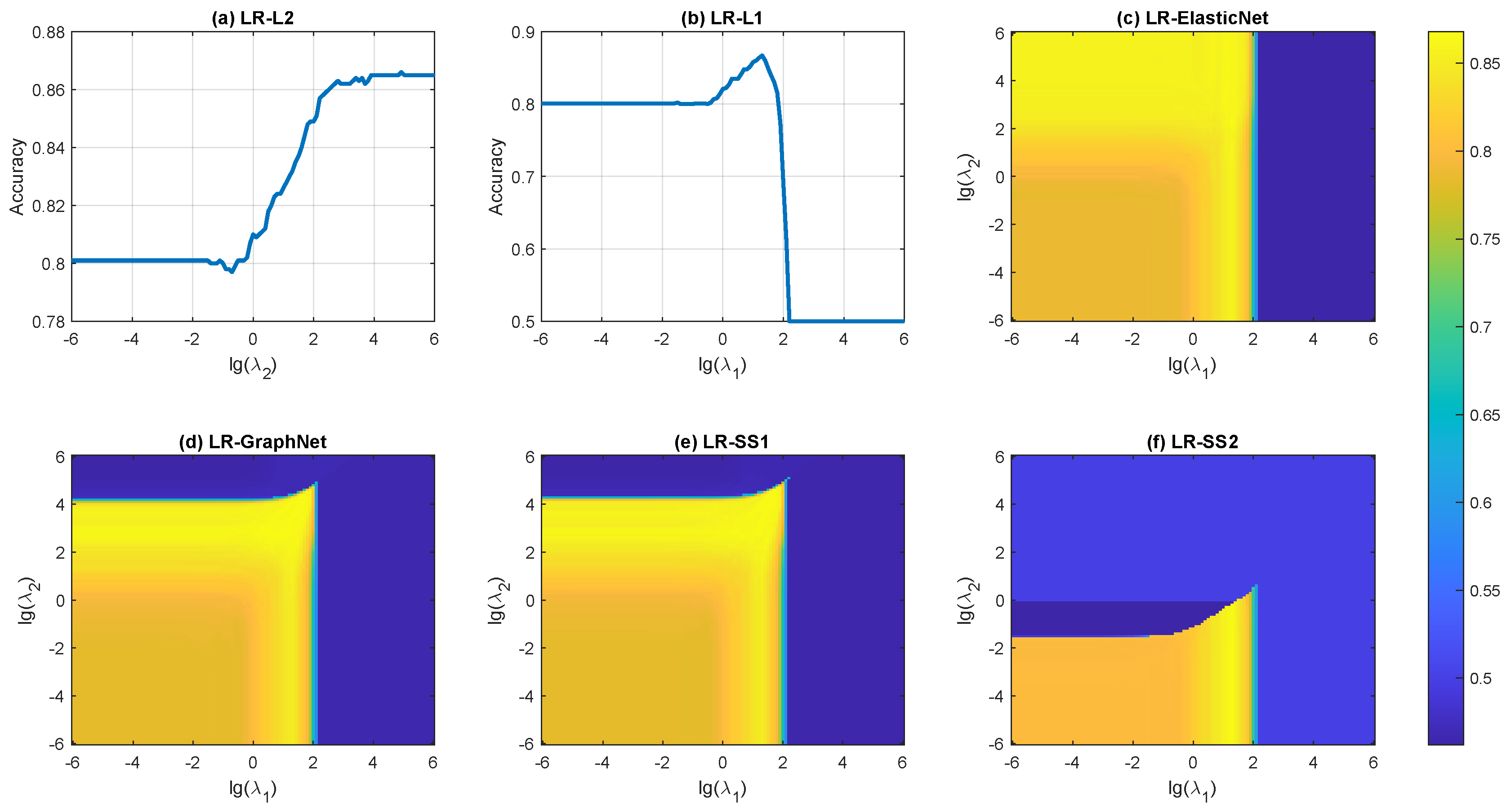
Figure 4 illustrates the relationship between classification accuracy and the parameters $lg\left({\lambda }_1\right)$ and $lg\left({\lambda }_2\right)$ across different algorithms. The visualizations reveal distinct patterns in how the accuracy responds to parameter variations, providing insights into each algorithm’s sensitivity to its regularization parameters.

For LR-L2 (Figure 4(a)), we observe three distinct regions in the accuracy curve. When $lg\left({\lambda }_2\right)\le -0.3$, the accuracy plateaus at approximately 0.801, indicating minimal impact of L2 regularization. As $lg\left({\lambda }_2\right)$ increases beyond this threshold, the accuracy shows a consistent upward trend, demonstrating the beneficial effect of stronger L2 regularization. Finally, when $lg\left({\lambda }_2\right)\ge 3.9$, the accuracy stabilizes around 0.865, suggesting that further increasing the regularization strength yields diminishing returns. The optimal performance is achieved at $lg\left({\lambda }_2\right)=4.9$ with an accuracy of 0.866.

For LR-L1 (Figure 4(b)), the accuracy exhibits a more complex pattern. When $lg\left({\lambda }_1\right)\le -0.4$, the accuracy remains constant at approximately 0.801, similar to the unregularized case. As $lg\left({\lambda }_1\right)$ increases, the accuracy follows an inverted U-shaped curve, first improving as the L1 regularization encourages sparsity, then declining as excessive sparsity begins to degrade performance. The accuracy reaches its peak of 0.867 at $lg\left({\lambda }_1\right)=1.3$, before eventually stabilizing around 0.500 when $lg\left({\lambda }_1\right)\ge 2.2$, where the strong L1 penalty forces most coefficients to zero.

For the algorithms with two parameters (Figure 4(c)-(f)), we can observe that when $lg\left({\lambda }_1\right)\ge 2.2$, the classification accuracy is consistently low, aligning with the results shown in Figure 4(b). When $lg\left({\lambda }_1\right)$ takes a relatively small value, e.g., $-6\le lg\left({\lambda }_1\right)\le 0$, the weight of sparse regularization becomes very low, and LR-ElasticNet approximates LR-L2. As shown in Figure 4(c), under these circumstances, the trend of classification accuracy with respect to $lg\left({\lambda }_2\right)$ is consistent with the results in Figure 4(a).

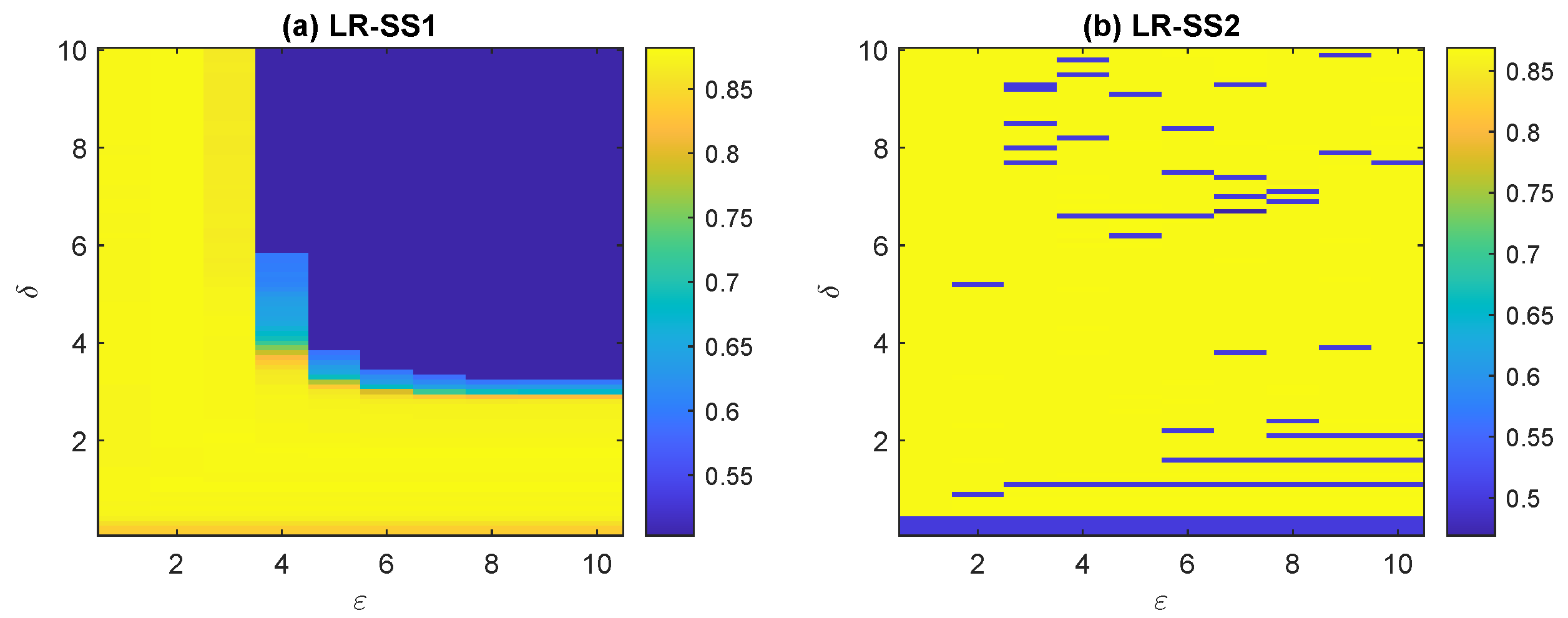
However, for the other three algorithms, i.e., LR-GraphNet, LR-SS1, and LR-SS2, when $lg\left({\lambda }_1\right)$ is very small and sparse regularization has minimal effect, what remains is not L2-norm regularization but rather smooth regularization with different types. In these cases, the trend of classification accuracy with respect to $lg\left({\lambda }_2\right)$ no longer aligns with the results shown in Figure 4(a) and Figure 4(c). For LR-GraphNet and LR-SS1, when $lg\left({\lambda }_2\right)\ge 4.5$, the classification accuracy is generally low in most cases. However, there are exceptions: when $lg\left({\lambda }_2\right)\ge 4.5$ and $0<lg\left({\lambda }_1\right)<2$, some parameter combinations can achieve relatively high classification accuracy. For LR-SS2, when $lg\left({\lambda }_2\right)\ge -1.1$, the classification accuracy is generally low in most cases. Similarly, there are exceptions: when $lg\left({\lambda }_2\right)\ge -1.1$ and $0<lg\left({\lambda }_1\right)<2$, some parameter combinations can achieve relatively high classification accuracy. These differences primarily arise from the use of different smooth regularizations.

Among the algorithms with two or more parameters, LR-ElasticNet achieves a classification accuracy of 0.875 at its optimal parameter values of $lg\left({\lambda }_1\right)=1.3$ and $lg\left({\lambda }_2\right)=2.1$. LR-GraphNet shows improved performance with an accuracy of 0.881 when $lg\left({\lambda }_1\right)=0.7$ and $lg\left({\lambda }_2\right)=2.7$. For the more complex algorithms LR-SS1 and LR-SS2, which each incorporate four tuning parameters (${\lambda }_1$, ${\lambda }_2$, $\delta$, and $\epsilon$), we fixed $\delta =1$ and $\epsilon =3$ while optimizing the remaining parameters. Under these conditions, LR-SS1 achieves the highest overall accuracy of 0.882 with $lg\left({\lambda }_1\right)=1.6$ and $lg\left({\lambda }_2\right)=4.0$, while LR-SS2 reaches an accuracy of 0.868 with $lg\left({\lambda }_1\right)=1.3$ and $lg\left({\lambda }_2\right)=-0.6$.

Table 6 shows the highest classification accuracies of the seven comparative algorithms and their corresponding optimal parameters.

The classification accuracy of LR is the lowest (0.801) among all methods, demonstrating that regularization techniques, whether L2-norm, sparsity, or smoothness constraints, effectively prevent overfitting and enhance the generalization performance of the algorithms. This aligns with statistical learning theory, where regularization helps control model complexity and reduces variance in predictions.

Comparing LR-L2 and LR-L1, which each contain only one regularization term, LR-L1 achieves a slightly higher classification accuracy (0.867) than LR-L2 (0.866). This suggests that the sparsity constraint (L1-norm) is marginally more effective than the L2-norm regularization in this case.

LR-ElasticNet combines L1-norm and L2-norm regularization, achieving a higher classification accuracy (0.875) than both LR-L1 and LR-L2. This improvement demonstrates the benefits of combining different types of regularization. LR-GraphNet further improves upon this by incorporating spatial smoothness constraints, reaching an even higher accuracy of 0.881.

LR-SS1 achieves the highest classification accuracy (0.882) among all methods, showing the effectiveness of combining sparsity with the proposed smooth regularization. However, it’s noteworthy that LR-SS2 achieves a lower accuracy (0.868) than LR-SS1, and when LR-SS2 reaches its optimal accuracy, the value of ${\lambda }_2$ is relatively small ($lg\left({\lambda }_2\right)=-0.6$). This suggests that for this particular dataset, the specific form of smooth regularization used in LR-SS2 may not provide as much benefit as the form used in LR-SS1.

To investigate the impact of parameters $\delta$ and $\epsilon$ on the performance of LR-SS1 and LR-SS2, we fixed $lg\left({\lambda }_1\right)$ and $lg\left({\lambda }_2\right)$ at their optimal values from Table 6 and varied $\delta$ from 0.1 to 10 in increments of 0.1, and $\epsilon$ from 1 to 10 in integer steps. Since we are dealing with one-dimensional signals where the distances between features are integers, $\epsilon$ is restricted to positive integer values. No such restriction applies to $\delta$, allowing it to take decimal values.

These results, shown in Figure 5, indicate reasonable parameter ranges for both algorithms. For LR-SS1, the classification accuracy remains close to the highest accuracy of 0.882 when $\epsilon =1$, 2, or 3, or when $\delta \le 2.7$. For LR-SS2, the classification accuracy stays close to its peak value of 0.868 when $\delta \ge 0.5$ for most cases. These patterns suggest that both algorithms exhibit robustness across certain ranges of parameter values.

It’s worth noting that potentially higher classification accuracies could be achieved for LR-SS1 and LR-SS2 through comprehensive optimization of all parameters simultaneously. However, such exhaustive parameter tuning was not conducted in our experiments due to computational constraints. A complete grid search across the four-dimensional parameter space (${\lambda }_1$, ${\lambda }_2$, $\delta$, and $\epsilon$) would be prohibitively expensive. Instead, we employed the above two-stage optimization approach. While this approach may not guarantee a global optimum, it offers an effective compromise between computational efficiency and model performance, enabling us to systematically analyze the influence of each parameter pair.

3.1.2. Feature Extraction Performance on the Simulated Dataset

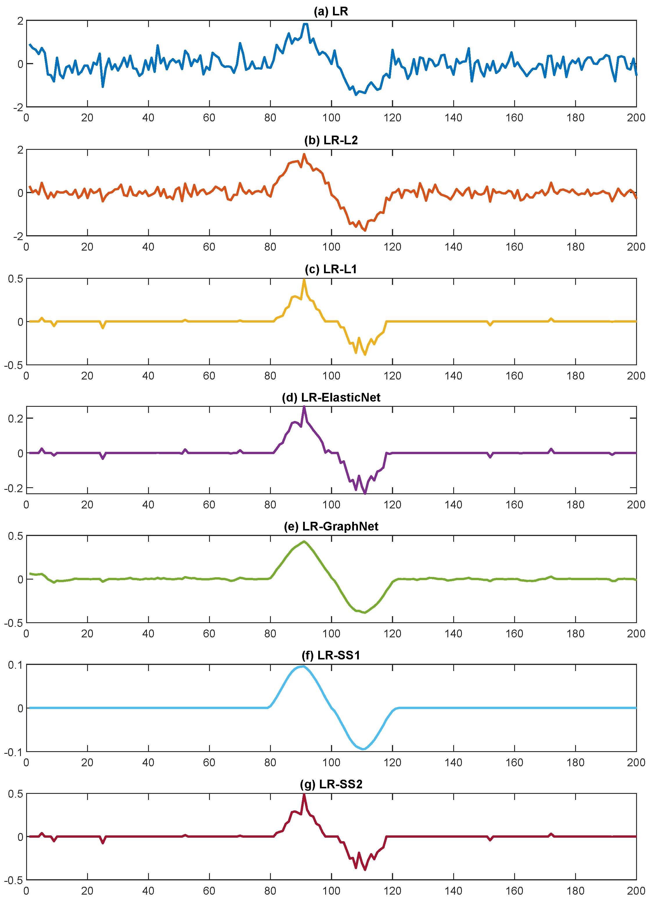
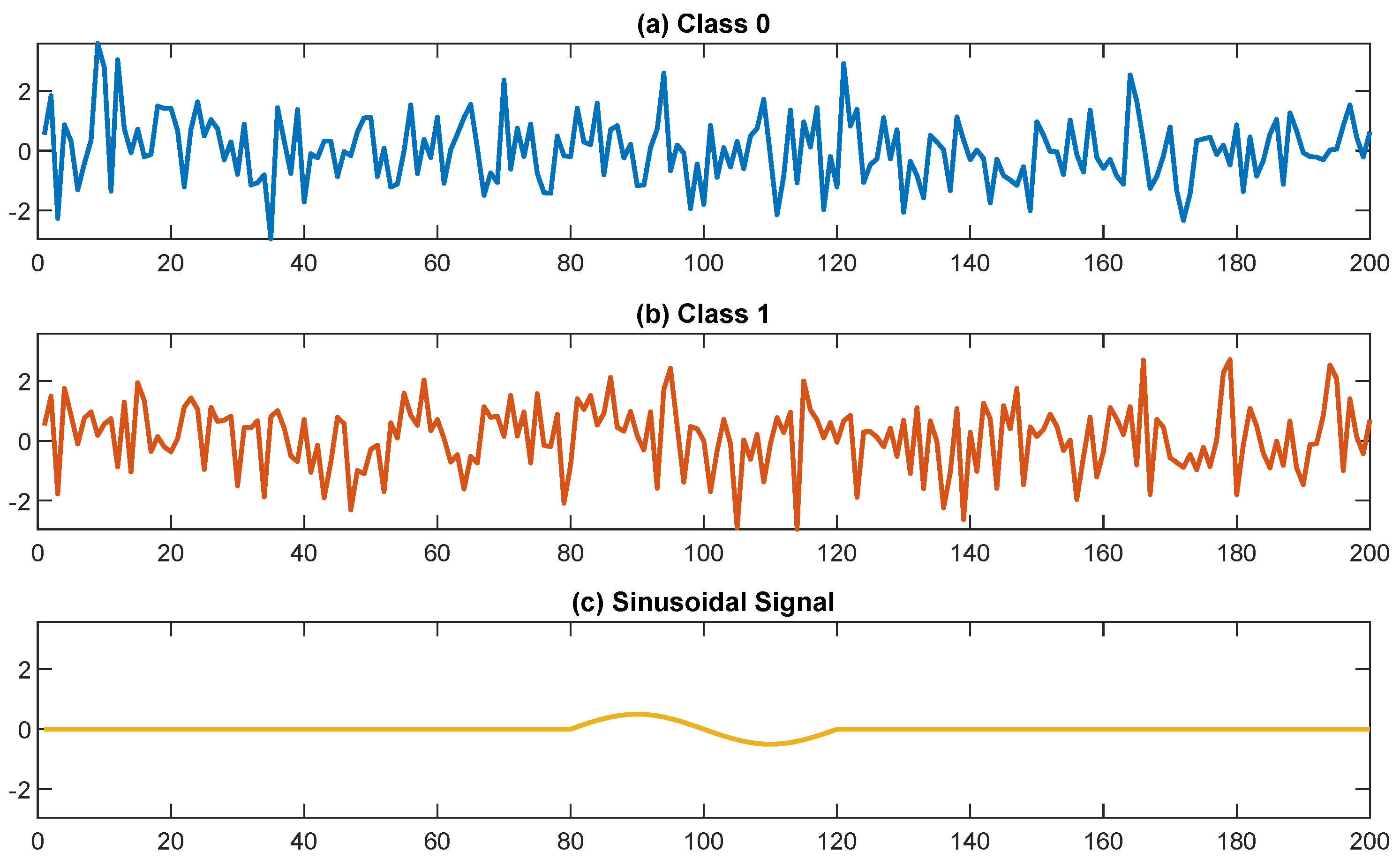
Figure 6 presents the weight vectors obtained using optimal parameters from Table 6 for each LR algorithm. The weight vectors from LR and LR-L2 lack both smoothness and sparsity, exhibiting noisy, non-zero values throughout the feature space. In contrast, LR-L1, LR-ElasticNet, LR-GraphNet, LR-SS1, and LR-SS2 demonstrate effective sparsity by reducing numerous weights to zero. Among these sparse solutions, LR-GraphNet and LR-SS1 are particularly noteworthy for their excellent smoothness properties. LR-SS1 proves to be the most effective method, producing weight vectors that closely resemble ideal sinusoidal signals by successfully zeroing out irrelevant regions while maintaining smooth transitions in the sinusoidal regions. This demonstrates an optimal balance between sparsity and smoothness constraints. LR-GraphNet achieves the second-best performance, exhibiting good sparsity and smoothness characteristics, although it retains some non-zero values outside the sinusoidal regions and shows slightly less smooth patterns compared to LR-SS1.

The remaining algorithms, namely LR-L1, LR-ElasticNet, and LR-SS2, exhibit comparable sparsity characteristics, demonstrating successful identification and preservation of specific patterns while effectively eliminating irrelevant features. The weight pattern obtained by LR-ElasticNet bears a strong resemblance to that of LR-L1, which can be attributed to the dominance of the sparsity regularization over the L2-norm regularization. Similarly, LR-SS2 produces results analogous to LR-L1, primarily due to its small optimal ${\lambda }_2$ value, which substantially reduces the influence of smooth regularization while preserving robust sparsity constraints. However, the patterns extracted through these algorithms lack the refined smoothness characteristics exhibited by LR-SS1 and LR-GraphNet, highlighting the critical role of effective smoothness regularization in accurately capturing the underlying signal structure.

Table 7 presents the sparsity and smoothness metrics for each method. LR and LR-L2 show no sparsity (0%), with all elements being non-zero. Among the sparse methods, LR-SS2 achieves the highest sparsity (80.5%), followed closely by LR-L1 (80.0%), LR-SS1 (79.5%) and LR-ElasticNet (77.0%). LR-GraphNet shows notably lower sparsity (31.5%), indicating it retains more non-zero elements than other sparse methods.

Examining the relationship between sparsity from Table 7 and regularization parameters from Table 6, we observe that sparsity is strongly correlated with the magnitude of ${\lambda }_1$. Generally, larger values of ${\lambda }_1$ lead to increased sparsity in the weight vector. In contrast, the relationship between sparsity and ${\lambda }_2$ is more nuanced. While the impact of ${\lambda }_2$ is considerably less significant compared to that of ${\lambda }_1$, it still influences sparsity to some extent. A notable example is LR-SS1. Despite having the largest ${\lambda }_1$ value among all methods, its relatively large ${\lambda }_2$ value results in a sparsity level that is slightly lower than both LR-SS2 and LR-L1. This suggests that strong smoothness regularization can partially counteract the sparsifying effect of ${\lambda }_1$, leading to solutions that maintain more non-zero elements to achieve smoother transitions in the weight vector.

Regarding smoothness, LR-SS1 demonstrates superior performance with the lowest smoothness value (0.4), closely followed by LR-GraphNet (0.5). This aligns with the core objectives of these methods, which explicitly incorporate smoothness regularization terms. The enhanced smoothness of LR-SS1 can be attributed to its larger ${\lambda }_2$ parameter compared to LR-GraphNet, resulting in more aggressive smoothness regularization. LR-L1, LR-ElasticNet, and LR-SS2 exhibit moderate smoothness values (all 1.2), with their sparsity-inducing regularization terms effectively zeroing many weights, leading to improved smoothness compared to LR-L2. In the case of LR-SS2, its relatively small ${\lambda }_2$ value limits the impact of the smoothness regularization term, resulting in smoothness characteristics similar to LR-L1 and LR-ElasticNet. The unregularized LR method shows the highest smoothness value (13.1), indicating sharp transitions between adjacent weights and highlighting how any form of regularization tends to improve weight vector smoothness.

The smoothness analysis clearly demonstrates the value of incorporating dedicated smoothness regularization terms. Methods employing explicit smoothness regularizations (LR-SS1 and LR-GraphNet) achieve markedly lower smoothness values compared to methods using only sparsity regularization (LR-L1) or no regularization (LR). This indicates that smoothness regularization terms effectively promote gradual transitions between adjacent weights, contributing to models that are potentially more interpretable and robust. The results suggest that when smooth weight patterns are desired, methods with dedicated smoothness regularization terms should be preferred over those focusing solely on sparsity or using no regularization.

3.2. Classification Performance on Simulated Datasets with Various Signal-to-Noise Ratios

To provide a more rigorous evaluation of the LR algorithms’ performance, we conducted additional experiments addressing two key limitations of our previous analysis: the use of a fixed dataset and the separate optimization of parameters for algorithms with four parameters (LR-SS1 and LR-SS2). We employed Bayesian optimization [51,52] for simultaneous parameter tuning and evaluated performance across multiple randomly generated datasets with varying signal-to-noise ratios.

Specifically, we generated four distinct synthetic datasets, each containing two classes with 1000 samples per class. For all datasets, Class 0 samples consisted of pure Gaussian noise (mean 0, variance 1). Class 1 samples were generated by superimposing a sinusoidal signal onto Gaussian noise (mean 0, variance 1). To systematically evaluate algorithm robustness across varying signal-to-noise ratios, we created the four datasets by setting the sinusoidal signal amplitude to 1, 1/2, 1/4, and 1/8, respectively. The sinusoidal signal was present between time points 80 and 120, consistent with our earlier experiments. For clarity, we refer to these four datasets as Dataset 1 (amplitude = 1), Dataset 2 (amplitude = 1/2), Dataset 3 (amplitude = 1/4), and Dataset 4 (amplitude = 1/8) in order of decreasing signal strength. This systematic variation in signal amplitude allows us to evaluate how each method performs as the classification task becomes increasingly challenging.

For each dataset, we first employed stratified sampling to split the 2000 samples evenly into training and test sets of 1000 samples each. The training set was then further divided using stratified sampling, with 80% used for training and 20% for validation. We used Bayesian optimization [51,52] to tune the parameters, with the number of iterations varying based on the algorithm complexity: 50 iterations for single-parameter algorithms (LR-L2, LR-L1), 100 iterations for two-parameter algorithms (LR-ElasticNet, LR-GraphNet), and 200 iterations for four-parameter algorithms (LR-SS1 and LR-SS2). After obtaining the optimal parameters, we retrained the models using the combined training and validation sets and evaluated their performance on the test set. To ensure robust statistical results, we repeated this entire process 100 times.

Table 8 presents comprehensive performance metrics across the four synthetic datasets, with signal amplitudes decreasing from 1 to 1/8 (Datasets 1-4). For each method and metric, we report the mean and standard deviation over 100 iterations. The results reveal several important patterns. LR-SS1 and LR-GraphNet consistently outperform other methods across all signal amplitudes, with nearly identical performance metrics. Their advantage is particularly evident as signal strength decreases. Specifically, for Dataset 4 (amplitude = 1/8), LR-SS1 and LR-GraphNet achieve accuracies of $(0.605\pm 0.013)$ and $(0.604\pm 0.012)$ respectively, while all other methods fall below 0.585. The small standard deviations (generally $\le 0.015$) across metrics demonstrate robust performance across different data splits and initializations. As expected, classification performance declines with decreasing signal amplitude, from approximately 0.985 accuracy in Dataset 1 to 0.605 in Dataset 4. However, the relative superiority of LR-SS1 and LR-GraphNet persists across all signal levels.

Figure 7 illustrates these trends in classification accuracy across datasets. The plot reveals excellent performance by all methods on Dataset 1 (accuracy > 0.96), with increasing differentiation as signal strength decreases. Error bars (one standard deviation) demonstrate result consistency across iterations. The visualization emphasizes the sustained performance advantage of LR-SS1 and LR-GraphNet, which becomes more pronounced at lower signal amplitudes. Their narrow error bars further highlight their stability relative to other approaches.

From Table 8 and Figure 7, we can observe that the classification accuracy of LR-SS2 is generally comparable to algorithms without smooth regularizations, including LR-L2, LR-L1, and LR-ElasticNet. These algorithms all show notably lower performance compared to the other two algorithms that incorporate smooth regularizations, namely LR-GraphNet and LR-SS1. Similar conclusions can be drawn from the weight matrices shown in Figure 6. Therefore, the smooth matrix ${\mathbf{Q}}^{\left(2\right)}$ in LR-SS2 is less effective in capturing the temporal or spatial structure of the data for classification and feature extraction purposes, as compared to the smooth matrix ${\mathbf{Q}}^{\left(1\right)}$ in LR-GraphNet and LR-SS1.

When comparing LR-GraphNet and LR-SS1, an interesting observation emerges. While LR-SS1 is theoretically a generalized form of LR-GraphNet and should achieve equal or better classification accuracy with optimal parameter tuning, our experimental results show that their performances are remarkably similar, with LR-GraphNet occasionally achieving marginally better results. This observation warrants discussion from two perspectives. First, it demonstrates the robust performance of the simpler LR-GraphNet model, suggesting that its more constrained parameter space may actually be advantageous in some scenarios. Second, despite employing extensive Bayesian optimization (100 iterations for LR-GraphNet and 200 for LR-SS1), the challenge of simultaneously optimizing four parameters in LR-SS1 versus two in LR-GraphNet highlights the practical limitations of parameter optimization in higher-dimensional spaces, even with sophisticated techniques.

In total, these findings strongly support the effectiveness and robustness of the LR-SS framework, especially LR-GraphNet and LR-SS1, under varying noise conditions. The thorough parameter optimization via Bayesian optimization ensures a fair comparison of each method’s capabilities, strengthening our conclusions about their relative performance.

3.3. Classification Performance on Real Datasets

Next, we evaluated the classification performance of the LR algorithms on the four real-world datasets. Following our experimental protocol from the synthetic datasets, we split the original training set of each real-world dataset into 80% training and 20% validation data, then utilized Bayesian optimization for parameter tuning. The numbers of optimization iterations were scaled according to each algorithm’s parameter complexity likewise. Once optimal parameters were determined, we retrained each model on the combined training and validation data with optimal parameters, and then evaluated on the test set. To ensure robust results, we conducted 30 repetitions of this process for the one-dimensional datasets (DistalPhalanxOutlineCorrect and GunPoint). For the computationally intensive image datasets (FashionMNIST and MNIST), which have larger sample sizes and higher dimensionality, we only performed 10 repetitions. Table 9 presents the comprehensive classification performance metrics for all four real-world datasets. Figure 8 illustrates the classification accuracy across the four real-world datasets, with error bars indicating one standard deviation.

The results in Table 9 and Figure 8 reveal several interesting patterns across the four real-world datasets. For the DistalPhalanxOutlineCorrect dataset, LR-GraphNet achieves the best overall performance with the highest accuracy (0.567 ± 0.110), recall (0.701 ± 0.208), F1 score (0.641 ± 0.132), and AUC (0.584 ± 0.098), while LR-SS2 leads in precision (0.606 ± 0.063). The performance advantage of LR-GraphNet and LR-SS1 over traditional methods is particularly notable, suggesting that incorporating structural information is beneficial for bone outline classification.

For the GunPoint dataset, LR-SS1 demonstrates superior performance across all metrics, achieving the highest accuracy (0.786 ± 0.051), precision (0.777 ± 0.058), recall (0.819 ± 0.074), F1 score (0.795 ± 0.048), and AUC (0.848 ± 0.072). This consistent dominance indicates that LR-SS1’s ability to capture temporal dependencies is particularly effective for motion classification tasks.

For the FashionMNIST dataset, both LR-L2 and LR-SS1 share the highest accuracy (0.978 ± 0.004) and F1 score (0.978 ± 0.004), while LR-ElasticNet leads in precision (0.981 ± 0.010) and LR-SS1 in recall (0.977 ± 0.002). LR-L2, LR-GraphNet, and LR-SS1 achieve comparable AUC scores (0.995 ± 0.003, 0.995 ± 0.003, and 0.994 ± 0.003 respectively), suggesting that for this relatively simple binary classification task, i.e., T-shirts vs. trousers, even traditional regularization methods perform well.

For the MNIST dataset, LR-L2 achieves the highest accuracy (0.997 ± 0.002) and precision (0.996 ± 0.004), while LR-GraphNet and LR-SS1 share the highest recall (0.999 ± 0.001). The AUC scores are consistently high (0.998 ± 0.003) across LR-L2, LR-ElasticNet, LR-GraphNet, and LR-SS1, indicating that distinguishing between digits 0 and 1 is a relatively straightforward task where most methods perform exceptionally well.

Overall, these results demonstrate that the LR-SS framework, particularly LR-GraphNet and LR-SS1, performs competitively or superiorly across diverse real-world applications. Their effectiveness is most pronounced in tasks with clear structural dependencies, such as the temporal patterns in GunPoint and the spatial patterns in DistalPhalanxOutlineCorrect. For simpler classification tasks like binary FashionMNIST and MNIST, the performance differences between methods become less pronounced, though the LR-SS variants still maintain competitive performance.

4. Discussion

In this study, we have introduced logistic regression with sparse and smooth regularizations (LR-SS), a novel framework that enhances traditional logistic regression by incorporating both sparsity and smoothness constraints. Our approach generalizes existing methods like GraphNet and SSLR by proposing three types of smooth regularizations that effectively capture the spatio-temporal structure of data. The framework provides a unified solution that can naturally reduce to these existing algorithms as special cases through parameter adjustment.

The experimental results demonstrate the superior performance of LR-SS compared to conventional logistic regression algorithms across both simulated and real-world datasets. For simulated data, LR-SS achieved consistently higher classification accuracy while extracting features that better preserve the underlying temporal and spatial patterns. In real-world applications, particularly the GunPoint and DistalPhalanxOutlineCorrect datasets, LR-SS variants showed remarkable improvements in classification metrics, with LR-GraphNet achieving the highest accuracy (0.567 ± 0.110) on the DistalPhalanxOutlineCorrect dataset and LR-SS1 achieving the highest accuracy (0.786 ± 0.051) on the GunPoint dataset. These results validate our framework’s ability to effectively balance sparsity and smoothness constraints while maintaining high predictive power.

A key technical contribution of our work is the development of an efficient vectorized iterative solution within the MM framework. This computational advancement, combined with simplified iterative solutions for GraphNet and Laplacian Matrix-based smooth matrices, significantly reduces the computational overhead typically associated with such complex regularization schemes. The algorithm’s guaranteed convergence to a local optimum provides theoretical soundness to our approach.

The extracted feature vectors from LR-SS exhibit improved interpretability through their sparse and smooth characteristics. This is particularly valuable in applications like medical diagnosis [14] and time series analysis [15], where understanding the underlying patterns is crucial. The framework’s ability to capture both temporal and spatial dependencies while maintaining sparsity offers a powerful tool for modern machine learning applications requiring both accurate prediction and interpretable feature extraction.

Future research directions could include: 1. Extending the framework to handle multi-class classification problems [9]. 2. Developing distributed computing solutions for large-scale applications [10]. 3. Introducing Lp-norm [53,54] into both the sparse and smooth regularization terms to improve the algorithms’ classification and feature extraction performance. 4. Investigating adaptive parameter selection methods for the regularization terms [55]. 5. Integrating the framework with deep learning architectures [33,34,35,36] for handling non-linear relationships.

5. Conclusion

This paper presents LR-SS as a comprehensive framework that advances the state-of-the-art in regularized logistic regression. By effectively combining sparsity and smoothness constraints, our approach achieves superior classification performance while maintaining feature interpretability. The framework’s ability to generalize existing methods and its efficient computational implementation make it a practical tool for real-world applications.

Our extensive experimental evaluation demonstrates that LR-SS significantly outperforms conventional methods across diverse datasets, particularly in scenarios with inherent temporal or spatial structure. The framework’s success in extracting meaningful, interpretable features while maintaining high predictive accuracy addresses a crucial need in modern machine learning applications.

The proposed vectorized iterative solution within the MM framework, along with specialized solutions for different smooth matrices, provides an efficient and theoretically sound approach to solving the optimization problem. This computational efficiency, combined with the framework’s flexibility in handling various types of structural information, makes LR-SS a valuable addition to the machine learning toolkit.

Looking forward, the principles and methods developed in this work can be extended to address increasingly complex classification challenges across various domains. The framework’s ability to balance sparsity, smoothness, and classification accuracy while maintaining computational efficiency positions it as a promising approach for future research and applications in machine learning, bioinformatics, and beyond.

References

1. Hosmer, D.W., Jr.; Lemeshow, S.; Sturdivant, R.X. Applied logistic regression; John Wiley & Sons, 2013. [Google Scholar]
2. Abdalrada, A.S.; Yahya, O.H.; Alaidi, A.H.M.; Hussein, N.A.; Alrikabi, H.T.; Al-Quraishi, T.A.Q. A predictive model for liver disease progression based on logistic regression algorithm. Periodicals of Engineering and Natural Sciences (PEN) 2019, 7, 1255–1264. [Google Scholar] [CrossRef]
3. Shipe, M.E.; Deppen, S.A.; Farjah, F.; Grogan, E.L. Developing prediction models for clinical use using logistic regression: an overview. Journal of thoracic disease 2019, 11, S574. [Google Scholar] [CrossRef]
4. Cowling, T.E.; Cromwell, D.A.; Bellot, A.; Sharples, L.D.; van der Meulen, J. Logistic regression and machine learning predicted patient mortality from large sets of diagnosis codes comparably. Journal of Clinical Epidemiology 2021, 133, 43–52. [Google Scholar] [CrossRef]
5. Goldstone, J.A.; Bates, R.H.; Epstein, D.L.; Gurr, T.R.; Lustik, M.B.; Marshall, M.G.; Ulfelder, J.; Woodward, M. A global model for forecasting political instability. American journal of political science 2010, 54, 190–208. [Google Scholar] [CrossRef]
6. Bhattacharjee, P.; Dey, V.; Mandal, U. Risk assessment by failure mode and effects analysis (FMEA) using an interval number based logistic regression model. Safety Science 2020, 132, 104967. [Google Scholar] [CrossRef]
7. Kemiveš, A.; Ranđelović, M.; Barjaktarović, L.; Đikanović, P.; Čabarkapa, M.; Ranđelović, D. Identifying Key Indicators for Successful Foreign Direct Investment through Asymmetric Optimization Using Machine Learning. Symmetry 2024, 16, 1346. [Google Scholar] [CrossRef]
8. Sutton, C.; McCallum, A.; et al. An introduction to conditional random fields. Foundations and Trends® in Machine Learning 2012, 4, 267–373. [Google Scholar] [CrossRef]
9. Krishnapuram, B.; Carin, L.; Figueiredo, M.A.; Hartemink, A.J. Sparse multinomial logistic regression: Fast algorithms and generalization bounds. IEEE transactions on pattern analysis and machine intelligence 2005, 27, 957–968. [Google Scholar] [CrossRef] [PubMed]
10. Liu, J.; Chen, J.; Ye, J. Large-scale sparse logistic regression. In Proceedings of the 15th ACM SIGKDD international conference on Knowledge discovery and data mining; 2009; pp. 547–556. [Google Scholar] [CrossRef]
11. Mohammadi, M.; Atashin, A.A.; Tamburri, D.A. An efficient projection neural network for ell_1-regularized logistic regression. arXiv 2021, arXiv:2105.05449. [Google Scholar] [CrossRef]
12. Shevade, S.K.; Keerthi, S.S. A simple and efficient algorithm for gene selection using sparse logistic regression. Bioinformatics 2003, 19, 2246–2253. [Google Scholar] [CrossRef] [PubMed]
13. Ryali, S.; Supekar, K.; Abrams, D.A.; Menon, V. Sparse logistic regression for whole-brain classification of fMRI data. NeuroImage 2010, 51, 752–764. [Google Scholar] [CrossRef] [PubMed]
14. Zhang, X.; Zhang, Q.; Wang, X.; Ma, S.; Fang, K. Structured sparse logistic regression with application to lung cancer prediction using breath volatile biomarkers. Statistics in Medicine 2020, 39, 955–967. [Google Scholar] [CrossRef] [PubMed]
15. Xu, Y.; Du, P.; Robertson, J.; Senger, R. Sparse logistic regression on functional data. arXiv 2021, arXiv:2106.10583. [Google Scholar] [CrossRef]
16. Klimaszewski, J.; Sklyar, M.; Korzeń, M. Learning L1-penalized logistic regressions with smooth approximation. In Proceedings of the 2017 IEEE International Conference on INnovations in Intelligent SysTems and Applications (INISTA); IEEE, 2017; pp. 126–130. [Google Scholar] [CrossRef]
17. Grosenick, L.; Klingenberg, B.; Katovich, K.; Knutson, B.; Taylor, J.E. Interpretable whole-brain prediction analysis with GraphNet. NeuroImage 2013, 72, 304–321. [Google Scholar] [CrossRef] [PubMed]
18. de Brecht, M.; Yamagishi, N. Combining sparseness and smoothness improves classification accuracy and interpretability. NeuroImage 2012, 60, 1550–1561. [Google Scholar] [CrossRef]
19. Watanabe, T.; Kessler, D.; Scott, C.; Angstadt, M.; Sripada, C. Disease prediction based on functional connectomes using a scalable and spatially-informed support vector machine. Neuroimage 2014, 96, 183–202. [Google Scholar] [CrossRef] [PubMed]
20. Zhang, C.; Yao, L.; Song, S.; Wen, X.; Zhao, X.; Long, Z. Euler elastica regularized logistic regression for whole-brain decoding of fMRI data. IEEE Transactions on Biomedical Engineering 2017, 65, 1639–1653. [Google Scholar] [CrossRef] [PubMed]
21. Wen, Z.; Yu, T.; Yu, Z.; Li, Y. Grouped sparse Bayesian learning for voxel selection in multivoxel pattern analysis of fMRI data. NeuroImage 2019, 184, 417–430. [Google Scholar] [CrossRef] [PubMed]
22. Luo, X.; Chang, X.; Ban, X. Regression and classification using extreme learning machine based on L1-norm and L2-norm. Neurocomputing 2016, 174, 179–186. [Google Scholar] [CrossRef]
23. Fuhry, M.; Reichel, L. A new Tikhonov regularization method. Numerical Algorithms 2012, 59, 433–445. [Google Scholar] [CrossRef]
24. Koh, K.; Kim, S.J.; Boyd, S. An interior-point method for large-scale l1-regularized logistic regression. Journal of Machine learning research 2007, 8, 1519–1555. [Google Scholar]
25. Lee, S.I.; Lee, H.; Abbeel, P.; Ng, A.Y. Efficient l 1 regularized logistic regression. In Proceedings of the AAAI; 2006; Vol. 6, pp. 401–408. [Google Scholar]
26. Tibshirani, R. Regression shrinkage and selection via the lasso. Journal of the Royal Statistical Society Series B: Statistical Methodology 1996, 58, 267–288. [Google Scholar] [CrossRef]
27. Zou, H.; Hastie, T. Regularization and variable selection via the elastic net. Journal of the Royal Statistical Society Series B: Statistical Methodology 2005, 67, 301–320. [Google Scholar] [CrossRef]
28. Rao, A.; Lee, Y.; Gass, A.; Monsch, A. Classification of Alzheimer’s Disease from structural MRI using sparse logistic regression with optional spatial regularization. In Proceedings of the 2011 Annual International Conference of the IEEE Engineering in Medicine and Biology Society; IEEE, 2011; pp. 4499–4502. [Google Scholar] [CrossRef]
29. Malbasa, V.; Vucetic, S. Spatially regularized logistic regression for disease mapping on large moving populations. In Proceedings of the Proceedings of the 17th ACM SIGKDD international conference on Knowledge discovery and data mining; 2011; pp. 1352–1360. [Google Scholar] [CrossRef]
30. Meinshausen, N.; Bühlmann, P. High-dimensional graphs and variable selection with the lasso. 2006. [Google Scholar] [CrossRef]
31. Friedman, J.; Hastie, T.; Tibshirani, R. Sparse inverse covariance estimation with the graphical lasso. Biostatistics 2008, 9, 432–441. [Google Scholar] [CrossRef] [PubMed]
32. Belkin, M.; Niyogi, P. Laplacian eigenmaps for dimensionality reduction and data representation. Neural computation 2003, 15, 1373–1396. [Google Scholar] [CrossRef]
33. Said, A.; Bayrak, R.; Derr, T.; Shabbir, M.; Moyer, D.; Chang, C.; Koutsoukos, X. Neurograph: Benchmarks for graph machine learning in brain connectomics. Advances in Neural Information Processing Systems 2023, 36, 6509–6531. [Google Scholar]
34. Li, X.; Zhou, Y.; Dvornek, N.; Zhang, M.; Gao, S.; Zhuang, J.; Scheinost, D.; Staib, L.H.; Ventola, P.; Duncan, J.S. Braingnn: Interpretable brain graph neural network for fmri analysis. Medical Image Analysis 2021, 74, 102233. [Google Scholar] [CrossRef] [PubMed]
35. Yan, Y.; Zhu, J.; Duda, M.; Solarz, E.; Sripada, C.; Koutra, D. Groupinn: Grouping-based interpretable neural network for classification of limited, noisy brain data. In Proceedings of the Proceedings of the 25th ACM SIGKDD international conference on knowledge discovery & data mining; 2019; pp. 772–782. [Google Scholar] [CrossRef]
36. Cui, H.; Dai, W.; Zhu, Y.; Kan, X.; Gu, A.A.C.; Lukemire, J.; Zhan, L.; He, L.; Guo, Y.; Yang, C. Braingb: a benchmark for brain network analysis with graph neural networks. IEEE transactions on medical imaging 2022, 42, 493–506. [Google Scholar] [CrossRef]
37. Rudin, L.I.; Osher, S.; Fatemi, E. Nonlinear total variation based noise removal algorithms. Physica D: nonlinear phenomena 1992, 60, 259–268. [Google Scholar] [CrossRef]
38. Tibshirani, R.; Saunders, M.; Rosset, S.; Zhu, J.; Knight, K. Sparsity and smoothness via the fused lasso. Journal of the Royal Statistical Society Series B: Statistical Methodology 2005, 67, 91–108. [Google Scholar] [CrossRef]
39. Dohmatob, E.D.; Gramfort, A.; Thirion, B.; Varoquaux, G. Benchmarking solvers for TV-L1 least-squares and logistic regression in brain imaging. In Proceedings of the 2014 International Workshop on Pattern Recognition in Neuroimaging; IEEE, 2014; pp. 1–4. [Google Scholar] [CrossRef]
40. Hunter, D.R.; Lange, K. A tutorial on MM algorithms. The American Statistician 2004, 58, 30–37. [Google Scholar] [CrossRef]
41. Lange, K. MM optimization algorithms; SIAM, 2016. [Google Scholar]
42. Fan, R.E.; Chang, K.W.; Hsieh, C.J.; Wang, X.R.; Lin, C.J. LIBLINEAR: A library for large linear classification. the Journal of machine Learning research 2008, 9, 1871–1874. [Google Scholar]
43. Friedman, J.H.; Hastie, T.; Tibshirani, R. Regularization paths for generalized linear models via coordinate descent. Journal of statistical software 2010, 33, 1–22. [Google Scholar] [CrossRef] [PubMed]
44. Donoho, D.L. De-noising by soft-thresholding. IEEE transactions on information theory 1995, 41, 613–627. [Google Scholar] [CrossRef]
45. Pothen, A.; Simon, H.D.; Liou, K.P. Partitioning sparse matrices with eigenvectors of graphs. SIAM journal on matrix analysis and applications 1990, 11, 430–452. [Google Scholar] [CrossRef]
46. Cao, F.; Huang, H.; Pietka, E.; Gilsanz, V. Digital hand atlas and web-based bone age assessment: system design and implementation. Computerized medical imaging and graphics 2000, 24, 297–307. [Google Scholar] [CrossRef] [PubMed]
47. Davis, L.M. Predictive modelling of bone ageing. PhD thesis, University of East Anglia, 2013. [Google Scholar]
48. Ratanamahatana, C.A.; Keogh, E. Three myths about dynamic time warping data mining. In Proceedings of the 2005 SIAM international conference on data mining, SIAM; 2005; pp. 506–510. [Google Scholar] [CrossRef]
49. Xiao, H.; Rasul, K.; Vollgraf, R. Fashion-mnist: a novel image dataset for benchmarking machine learning algorithms. arXiv 2017, arXiv:1708.07747. [Google Scholar] [CrossRef]
50. LeCun, Y.; Bottou, L.; Bengio, Y.; Haffner, P. Gradient-based learning applied to document recognition. Proceedings of the IEEE 1998, 86, 2278–2324. [Google Scholar] [CrossRef]
51. Snoek, J.; Larochelle, H.; Adams, R.P. Practical bayesian optimization of machine learning algorithms. Advances in neural information processing systems 2012, 25. [Google Scholar]
52. Shahriari, B.; Swersky, K.; Wang, Z.; Adams, R.P.; De Freitas, N. Taking the human out of the loop: A review of Bayesian optimization. Proceedings of the IEEE 2015, 104, 148–175. [Google Scholar] [CrossRef]
53. Wang, J. Generalized 2-D principal component analysis by Lp-norm for image analysis. IEEE Transactions on Cybernetics 2015, 46, 792–803. [Google Scholar] [CrossRef] [PubMed]
54. Wang, J.; Xie, X.; Zhang, L.; Chen, X.; Yue, H.; Guo, H. Generalized Representation-based Classification by Lp-norm for Face Recognition. IAENG International Journal of Computer Science 2024, 51. [Google Scholar]
55. Tang, X.; Liu, S.; Nian, X.; Deng, S.; Liu, Y.; Ye, Q.; Li, Y.; Li, Y.; Yuan, T.; Sun, H. Improved adaptive regularization for simulated annealing inversion of transient electromagnetic. Scientific Reports 2024, 14, 5240. [Google Scholar] [CrossRef] [PubMed]
Figure 1. Illustration of smooth matrices. (a) Identity matrix. (b) Q ( 1 ) with δ = 0.8 and ε = 3 . (c) Q ( 1 ) with δ = 1.6 and ε = 3 . (d) Q ( 1 ) with ε = 1 . (e) Q ( 2 ) with δ = 0.8 and ε = 3 . (f) Q ( 2 ) with δ = 1.6 and ε = 3 .
Preprints 144028 g001
Figure 2. Simulated data showing two classes and the sinusoidal signal. (a) Class 0 (blue) consists of pure Gaussian noise, (b) Class 1 (red) consists of Gaussian noise superimposed with the sinusoidal signal, and (c) the sinusoidal signal. The sinusoidal signal is present with amplitude 1/2 between sample points 80 and 120.
Preprints 144028 g002
Figure 3. Examples from the four real-world datasets: (a) DistalPhalanxOutlineCorrect dataset showing one sample from each class (correct vs. incorrect outlines), (b) GunPoint dataset showing one trajectory from each class (gun-drawing vs. pointing), (c) FashionMNIST dataset showing six samples from each class (T-shirt/top vs. trouser), and (d) MNIST dataset showing six samples from each class (digits 0 vs. 1).
Preprints 144028 g003
Figure 4. Classification accuracy versus parameters for different algorithms: (a) LR-L2, (b) LR-L1, (c) LR-ElasticNet, (d) LR-GraphNet, (e) LR-SS1, (f) LR-SS2. For LR-SS1 and LR-SS2, the parameters δ and ε are fixed at 1 and 3 respectively.
Preprints 144028 g004
Figure 5. Classification accuracy of LR-SS1 with varying δ and ε , where lg ( λ 1 ) and lg ( λ 2 ) are fixed at their optimal values from Table 6.
Preprints 144028 g005
Figure 6. The weight vectors obtained with the optimal parameters from Table 6 for: (a) LR, (b) LR-L2, (c) LR-L1, (d) LR-ElasticNet, (e) LR-GraphNet, (f) LR-SS1, and (g) LR-SS2.
Preprints 144028 g006
Figure 7. Classification accuracy across datasets with varying signal amplitudes (1, 1/2, 1/4, and 1/8). Results show mean accuracy over 100 iterations, with error bars indicating one standard deviation.
Preprints 144028 g007
Figure 8. Classification accuracy across four real-world datasets. Results show mean accuracy over 30 iterations for the DistalPhalanxOutlineCorrect and GunPoint datasets, 10 iterations for the FashionMNIST and MNIST datasets, with error bars indicating one standard deviation.
Preprints 144028 g008