
Submitted:
06 October 2025
Posted:
08 October 2025
You are already at the latest version
Abstract
Multicollinearity is a common issue in regression analysis that occurs when some predictor variables are highly correlated, leading to unstable least squares estimates of model parameters. Various estimation strategies have been proposed to address this problem. In this study, we enhance a ridge-type estimator by incorporating pretest and shrinkage techniques. We conducted an analytical comparison to evaluate the performance of the proposed estimators in terms of bias, quadratic risk, and numerical performance using both simulated and real data. Additionally, we assessed several penalization methods and three machine-learning algorithms to facilitate a comprehensive comparison. Our results demonstrate that the proposed estimators outperform the standard ridge-type estimator with respect to mean squared error in simulated data and mean squared prediction error in real data applications.
Keywords:
Ridge-Type estimation
; shrinkage
; pretest
; penalization methods
; machine learning
1. Introduction
Regression analysis provides answers to queries concerning the dependence of a variable, known as the response, on one or a set of independent variables, known as predictors. These include problems like predicting the response value for a given collection of predictors or identifying the most significant group of predictors with a plausible impact on the response variable. A commonly used method to estimate the functional relationship between the response variable and the set of predictors is the ordinary least squares method (OLS). This method provides the best linear unbiased estimator (BLUE) of the regression vector of coefficients based on the Gauss-Markov theorem. This result holds, assuming the columns of the design matrix, which are represented by the independent variables, are not correlated. However, the OLS estimator becomes less efficient if a strong or near-to-strong linear relationship exists among the columns of design matrix, known as multicollinearity.
The multicollinearity issue lessens the accuracy of the OLS estimated coefficients, also the coefficient estimates can exhibit significant fluctuations depending on the inclusion of different independent variables in the model, beside to a high degree of sensitivity to even minor change in the regression model. There are several estimation methods developed to improve the OLS estimator when multicollinearity exists. For instance, Hoerl and Kennard [1] proposed the ridge regression estimator analytically and numerically the superiority of the new estimator over the OLS estimator. Later, Liu K [2] introduced a novel biased estimator and verified analytically and numerically the superiority of the new estimator over the OLS estimator known as Liu type estimator . Recently, Kibria and Lukman [3] developed a new ridge type estimator for the regression parameter vector. They showed the new estimator performed better than the ridge and Liu estimators in terms of the MSE criterion.
The OLS technique uses the sample information obtained from the data set to draw inference about the unknown population regression vector of parameters, which refers to classical inference method. However, in Bayesian context, the sample information is combined with non-sample information (NSI) to make an inference about the regression parameters. Such NSI may not be available at all times. However, model selection and building procedures as AIC, BIC, penalization methods, or machine learning algorithms could still be utilized to yield NSIs. Bancroft [4] was one of the first to try estimating regression coefficients by merging NSIs with sample information and produced what is known as the pretest estimator. The Pretest estimator relies on evaluating the statistical significance of certain regression coefficients. After the determination is made, the pretest selects either the estimate of the full model or the estimator of the revised model, known as sub-model, which has fewer number of coefficients. The pertest algorithm chooses either the full or sub model estimators using binary weights. A modified version of the pretest estimator, known as the shrinkage estimator, has been formulated by Stein [5]. This estimator utilizes smooth weights to merge the estimations from both the overall and sub-model estimators. The regression coefficients are modified to converge towards a desired value that is influenced by the NSI. Nevertheless, the enhanced shrinkage estimator sometimes encounters an occurrence of excessive reduction. Following that, a more improved version of this estimator is proposed by Stein [6] to efficiently address the issue of excessive shrinkage, known as the positive shrinkage estimator.
Many researches have been drawn to the idea of using shrinkage and pretest estimation approaches. For instance, [7] proposed a novel approach utilizing pretest and shrinkage approaches to accurately estimate the regression coefficients vector of the marginal model for multinomial responses. [8] presented the Liu-type pretest, shrinkage, and positive shrinkages estimators for the conditional autoregressive regression model’s large-scale effect parameter vector, and demonstrated that these estimators are more efficient than Liu-type estimators. By employing the concept of shrinkage, [9] proposed an enhanced version of the Liu-type estimator. The proposed method’s superiority was demonstrated using analytical and numerical data. Subsequently, [10] proposed the utilization of the ridge estimator as an appropriate method for managing high-dimensional multicollinear data. [11] proposed the use of pretest and shrinkage ridge estimation techniques for the linear regression model. Demonstrated the advantages of employing the suggested estimators alongside specific penalty estimators. [12] introduced the pretest and shrinkage approaches that use generalized ridge regression estimation to address issues related to multicollinearity and high-dimensional situations. [13] introduced an effective shrinkage and penalty estimators for regression coefficients in spatial error models. It showcases the efficiency improvements using asymptotic and numerical studies. In a recent study, [14] shown that the ridge-type pretest and shrinkage estimators outperformed the maximum likelihood estimator in the presence of multicollinearity in a spatial error regression model. To obtain further information on the shrinkage estimators, please consult with [15,16,17], among other relevant sources.
The primary objectives of this research are threefold. The initial goal of this study is to improve the ridge estimator (RE) proposed by [3] of the regression vector by integrating pretest and shrinkage approaches in the presence of multicollinearity among the regressor variables. This enhancement primarily focuses on situations where particular regression coefficients are considered insignificant. The second purpose is to examine the analytical findings on the bias and quadratic risks of the estimators for the newly proposed set. The third step involves evaluating the performance of the estimators by numerical simulation, specifically by measuring the mean squared error. Additionally, the estimators will be assessed using real-world data to determine the prediction error.
The subsequent sections of the paper are structured in accordance with our objectives. In Section (2), we provide the regression model and the KL estimator. The strategy improvements for the RE estimator are outlined in Section (3). In Section (4), we studied some analytical properties of the array of estimators, specifically the bias and quadratic risks. Some penalizing techniques are presented in Section (5), and we presented three machine learning algorithms in Section (6). In Section (7), we conducted a comparison of the array of estimators using both Monte Carlo simulation and a real data example. Section (8) provides concluding remarks, and a supplementary section is appended at the conclusion of the manuscript, which includes the proofs of the analytical findings.
2. Statistical Model and New Ridge Estimation
To explain the problem, let us consider the linear regression model given below
where is an vector of random responses, is an full rank design matrix with , is a vector of unknown but fixed regression parameters, and is an random error vector such that the expected value and the variance of are, respectively , and . The ordinary least squares (OLS) estimator of is given by:
where . Based on Gauss-Markov theorem, is the best linear unbiased estimator (BLUE) of , which is the case when the columns of the design matrix are not correlated, with . However, becomes less efficient if a strong or near to strong linear relationship exists among the columns of , which is known as multicollinearity. The ridge-type estimator proposed by [3] estimator of the regression coefficient is denoted by and given by:
where is a identity matrix and known as a biasing parameter to be estimated using the data.
The incorporation of NSI in a model often involves the inclusion of a hypothesized restriction on the model parameters, resulting in the emergence of potential sub-models. Bayesian statistical approaches have been developed in response to the need of incorporating NSI into models fitted to objective sample data. This allows for the consideration of the uncertainty introduced by both sources of information. If the NSI asserts that some of the regression coefficients are irrelevant, then it is possible to integrate this information into the estimation process via testing a linear hypothesis of the form:
where is a known matrix of rank , and is a vector of zeros.
The new sub-model often incorporates a reduced number of regression variables, facilitating interpretation and mitigating the complexity associated with a large number of irrelevant variables. A Candidate sub-model may be obtained by using some known variable selection methods, such as AIC , BIC, or by penalization techniques as ridge estimation, LASSO, Elastic net, SCAD, or adaptive LASSO, among others. Under the restriction given by the hypothesis in (3), and using Lagrange multipliers the sub-model estimator of , denoted by is given by:
Obviously, if the restriction in (3) is correct, then , which is unbiased estimator for . On the other hand, when the restriction is not true, becomes less efficient than , particularly in cases where there is ongoing multicollinearity among the columns of the columns. This can be diminished by employing the Kibria and Lukman estimation method to calculate the coefficients of sub-model regression, which will be denoted by and given as follows:
3. Strategy Improvements for the RE Estimator
Given that a sub-model has been acquired via the use of penalization methods or machine learning algorithms, we will explore various shrinkage and pretest procedures to combine the estimations from both the full and sub-models. First, we establish the definition of a test statistic, designated as , which is used to test the hypothesis stated in equation (3) as follows:
where is an estimator of . The test statistic , assuming the null hypothesis (3), is asymptotically distributed according to a distribution with degrees of freedom. However, if the alternative hypothesis holds, the test statistic follows a non-central distribution with a non-centrality parameter . An improved set of shrinkage estimators using [3] technique can be formulated as follows:
where is a Borel measurable function of and certain selections of may provide shrinkage estimators that are both plausible and helpful.
3.1. Preliminary and Shrinkage Estimators
The preliminary test estimator can be obtained by when the function , it is denoted by , and given by:
where, is the indicator function, is the level of significance, and represents the upper critical value of the distribution with degrees of freedom. Clearly, if the indicator function is zero, then , otherwise . One limitation of this estimator is its reliance on a binary choice of the two estimators that is influenced by the level of significance . A more refined method of assigning weights may be attained by setting the James-Stein shrinkage estimator, which is formally stated as follows.
The shrinkage estimator experiences over-shrinkage, resulting in negative coordinates when . The positive James–Stein estimator solves this issue. It is denoted by , and can by obtained by setting
which can be simplifies as:
3.2. Modified Preliminary and Shrinkage Estimators
Another way to enhance the regression estimate when the null hypothesis in (3) is true, which could any type of NSI, is to consider the linear shrinkage estimator of the sub and full models RE estimator, [25] provided evidence that the estimator is competitive when the NSI is correct. The estimator, denoted by , and given by:
where serves as a tuning parameter which is selected to minimize the estimator’s mean-squared error. Obviously, when , , and when , . Additionally, we can employ the idea proposed by [26] to produces a new RE estimator that is often referred to as the shrinkage pretest estimator. It is denoted by and given as follows:
4. Analytical Properties
This section presents the bias and quadratic risk functions of the proposed RE estimators. For this purpose, assume is any of these RE-type estimators; consequently the bias of will be . The bias expressions are given in the following theorem.
Theorem 1
Let , and , then:
where is the non-central cumulative distribution function of F random variable with degrees of freedom, is the critical value form the distribution, and as a non-centrality parameter. For the proof of the above theorem see the Appendix A.
In order to obtain the quadratic risk expressions, we use the quadratic loss function of any RE-type estimator , which is defined for any positive definite matrix as follows:
The quadratic risk function of any estimator, denoted by , and defined as . The quadratic risk expressions are given in the following theorem.
Theorem 2
In the following section, we shall enumerate some extant penalization methods to produce a new sub-model from the literature.
5. Some Penalizing Techniques
Penalty estimators are produced as a consequence of simultaneous model selection and parameter estimation processes by applying a penalty to the least squares equation. As a result, model selection and estimating processes are included in penalty techniques. Some of the penalty techniques are provided below.
5.1. Ridge Estimator
The ridge estimator proposed by [1], efficiently addresses the issue of multicollinearity by using a technique known as coefficient shrinkage, which reduces the magnitudes of the coefficients associated with strongly correlated variables. This approach aids in achieving model stability and mitigating the influence of multicollinearity on the estimation of coefficients. It is denoted by , and can obtained by minimizing the penalized residual sum of squares, and it is given by:
where is a constant known as a biasing parameter.
5.2. LASSO Estimator
The LASSO or the least absolute selection and shrinkage operator proposed by [18]. It is a method for selecting variables and estimating parameters in linear models. In the usual least squares estimation of regression coefficients, the LASSO algorithm employs the norm of the vector to define a penalty term. The LASSO estimator, denoted by , and given by:
where is tuning parameter to be estimated from the data. However, it is known that the LASSO technique may not be the most ideal approach when dealing with a set of columns in a design matrix that exhibit significant levels of correlation. As a solution, [19] introduced the elastic net (ELNT) method, which combines an and penalty terms in a linear manner.
5.3. Elastic Net Estimator
It is denoted by and obtained as follows:
where , are respectively, the LASSO and the ridge tuning parameters. A variable selection process is said to possess the oracle property when it successfully identifies the correct subset of zero coefficients inside the regression model being examined. Additionally, the estimators of the remaining non-zero coefficients demonstrate consistency and asymptotic normality. The LASSO estimator does not enjoy this property. However, [20] and [21] developed two approaches that possess the oracle property . In the following two subsections, we establish the definitions for these methods.
5.4. SCAD Estimator
The SCAD or smoothly clipped absolute deviation estimator, denoted by and obtained by:
where is a continuous function of t and its derivative is given by:
where , are the known as tuning parameters. Note that when , the function is equivalent to penalty.
5.5. Adaptive LASSO Estimator
Using adaptive weights on penalties on regression coefficients, the adaptive LASSO modifies the LASSO penalty. Theoretically, it has been demonstrated that the adaptive LASSO estimator enjoys the oracle property. It is denoted by , and obtained by:
where is a weight function defined as . The estimator is considered to be root-n consistent for . The minimization process for the adaptive LASSO solution does not provide any computing challenges and can be easily solved. One possible choice for is OLS estimate of . Now, we will describe some machine learning algorithms that will be used in this manuscript.
6. Machine Learning
The area of regression analysis has been significantly transformed by the advent of machine learning, providing robust methodologies and strategies to extract meaningful insights and achieve precise predictions from intricate data sets. Yet, the emergence of machine learning has expanded the scope of regression analysis, allowing us to use the predictive capacities of algorithms in order to unveil latent patterns and make informed judgments based on data. Three machine learning algorithms are briefly described: Random forest, K-nearest neighbors, and neural network.
6.1. Random Forest
[27] suggested a technique for creating tree-based classifiers that may be expanded as needed to improve accuracy on both training and hidden data, which is known as random forest. Random Forest is one of the most effective and flexible algorithms that can be used for both classification and regression. It’s a kind of ensemble learning that takes the results of many different decision trees and uses them together to come up with more reliable results. It build several decision trees on distinct subsets of the training data, and let them generate their own predictions. Randomization is introduced via bootstrapping using random data points and training set replacements and selecting a random subset of features for each tree. Later on, [28] discussed the problem of over fitting and getting the most accurate results by building a decision tree-based predictor that stays as accurate as possible on training data and gets more accurate as it gets more complicated. In a Random Forest, the final prediction is derived by aggregating the predictions of all the individual trees, naturally through regression averaging. This ensemble method reduces over-fitting and increases the algorithm’s precision and stability. For more details about the extensions and developments of the algorithm can be found in [29] and [30], among others.
6.2. K-Nearest Neighbors
The K-nearest neighbor (KNN)is an effective machine-learning algorithm used for classification and regression as the Random Forest algorithm. It was initially proposed by [31], and later on, [32] made modifications to it. The KNN method employs a supervised learning in a non-parametric fashion. In the context of economic forecasting, [33] examined the application of the KNN method, and showed it exhibits greater efficacy compared to alternative methodologies. [34] examined the implementation of the Euclidean distance formula in KNN in comparison to the normalized Euclidean distance, Manhattan, and normalized Manhattan. [35] provided a comprehensive examination of several methodologies employed in Nearest Neighbour classification.
The KNN uses instance-based, non-parametric learning. The method does not rely heavily on assumptions about the underlying data distribution. However, it produces predictions via evaluating similarities between the data points. In regression context, The method computes the average or weighted average of the response value of the K nearest neighbours to predict the response value for the new data point. The KNN algorithm is often used for initial machine learning applications due to its simplicity in comprehension and implementation. Yet, the performance of the system may be influenced by the selection of K and the specific distance measure used. Moreover, the computational cost associated with this approach is high, since it necessitates the calculation of distances for every data point in the data set during the prediction stage.
6.3. Neural Network
A neural network is a computer model that draws inspiration from the anatomical and functional characteristics of the human brain. One of the firsts attempts about this method proposed by [36] who established the foundation for comprehending the ability of basic computational units, resembling neurons, to execute intricate logical operations. Subsequently, other improvements and enhancements have been incorporated into this approach. [37] introduced a detection approach based on a neural networks method for identifying changes in the properties of systems with unknown structures. [38] presented a case study showcasing the effective operation of neural networks in the evaluation of credit risk. [39] provided a thorough examination of clustering neural networks approaches based on competitive learning. [40] provided an overview of academic articles on neural networks that have been published in archival research journals from 1989 to 2000.
The neural network purpose is to effectively process information and acquire knowledge via the analysis of data. Neural networks are composed of linked nodes, which are arranged in layers. These networks have exceptional proficiency in addressing intricate issues, notably in domains like as pattern recognition, picture and audio recognition, natural language processing, and other related fields.
After obtaining a sub-model estimator in addition to the full model estimator, which contains all available variables , it becomes possible to assess the accuracy of the sub model using different criteria. The objective of this study is to identify estimators that are functions of both and with the purpose of mitigating the potential risks associated with either of these estimators over a wide range of parameter values. This objective can be accomplished by developing the pretest and shrinkage estimators in the subsequent section.
7. Numerical Illustrations
In this section, we will investigate the finite-sample properties of the proposed estimators using Monte Carlo simulation experiments and a real data example.
7.1. Simulation Experiments
The properties of the estimator under investigation and the standards being applied to evaluate the findings will determine how the simulation experiment should be prepared. Following Kibria and Lukman [3], the following equation was used to produce the regressor variables.
where are independent and identically standard normal random variables, and is the correlation between and for . The response variable is then obtained via the following equation:
where are , the regression vector is partitioned as , and let varies over the set , which represents the degree of deviation from the null hypothesis in (3). In this simulation, we choose , and set , . The correlation coefficient is chosen to vary over the set , , and . We set for testing the hypothesis in (3). It was seen that the performance of all estimators had a similar pattern when the values of , and q were varied. To save space, we have chosen , , , then we run the simulation for iterations for .
For each estimator, we compute the mean squared error (MSE) as follows:
where is any of the proposed estimators in this study.
For the purpose of comparison, we use the relative efficiency of the mean squared error (RE) with respect to which is defined as follows:
A number grater than one of the RE indicates the superiority of over , and vice versa. Figure 1 shows the graphs for the cases we considered. The following conclusion can be obtained.
- The sub-model estimate consistently beats the all other estimators when the null hypothesis in (3) is true or approximately true. However, its relative efficiency decreases and eventually approaches zero as increases. Moreover, all estimators outperform the regular estimator in terms of mean squared error across all values of .
- For all values of , the RE positive shrinkage estimator dominates all other estimators, except when the sub-model is true, in which case the RE sub-model and the pertest estimators outperformed it.
- The relative efficiencies exhibit a consistent pattern when the values of , and are held constant for both sample sizes used in this simulation.
7.2. Data Examples
In this section, we will consider a case study discussed by [41] in two different chapters of their book about and also available for free within the "VisCollin"-R-package by [43]. The data originally studied by [42]. His goal was to detect the key soil factors that affect the aerial biomass in the marsh grass Spartina alterniflora in the Cape Fear Estuary of North Carolina at different three locations. At each location, three types of Spartina vegetation areas were sampled, namely devegetated “dead” areas, short" Spartina areas, and "tall" Spartina areas. Five samples of the soil substrate from different sites were collected within each location-vegetation type. These samples were then evaluated for 14 different physico-chemical parameters of the soil monthly for several months, resulting in a total of 45 samples. There are 45 observations in this data set covering the 17 variables, the location loc, area type type, hydrogen sulfide , salinity in percentage SAL, ester-hydrolase Eh7, soil acidity in water pH, buffer acidity at pH 6.6 BUF, concentration of following elements: phosphorus P, potassium K, calcium Ca, magnesium Mg, sodium Na, manganese Mn, zinc Zn, copper Cu, ammonium NH4, and the arial biomass BIO as the repones variable.
One main objective is to employ the set of variables that can accurately predict the response variable. As a first investigation of multicollinearity, we construct the correlation plot among these variables which is given by below in Figure 2.
The plot shows that there are many significant relationships between these variables, and some of these relations are very strong and highly significant with . This indicates a multicollinearity exists among theses variables, which can be easily detected by the variance inflation factor plot given below in Figure 3.
The VIF plot shows a serious multicollinearity problem, as some of the value are more than 5 in many cases. Hence, the RE estimator will reduce this problem and produce a better estimates of the parameters. Moreover, the prossed estimators will be an additional improvement to estimate and predict the target response variable BIO.
In the absence of prior knowledge, the limitation on the parameters is established either through the judgment of an expert or by the utilization of existing methodologies for variable selection such as the Akaike information criteria (AIC), forward selection(FW), backward elimination(BE), best subset selection(BS), Bayes information criterion (BIC), or by some penalization algorithms as Lasso, Adaptive lasso and others to produce a sub model. In this example, we at first employ the forward, backward and best subset selection methods to produces a sub model, then obtain the RE, pretest, and shrinkage estimators. Secondly, we apply the random forest, K-nearest neighbors, and the neural network as a machine learning algorithms to compare the prediction error with the seven proposed estimators. The sub models selected by the forward, backward, and best subset selection are summarized in Table 1 below.
In our analysis, we will examine two sub models: the forward sub model, which includes with the intercept the variables pH, Ca, Mg, and Cu. The second one is the backward/best subset that includes with the intercept the variables SAL, K, Zn, Eh7, Mg, Cu, and NH4. The two sub models will be designated as Sub.1 and Sub.2, respectively.
We fit a full model with all available variables and the selected sub-model. The whole model yields an estimated value of . Kibria and Lukman [3] presented several methods for estimating the biasing parameter , but we choose the one with the lowest MSE, which also provided by [23]. The estimated value of is determined by writing the model in (1) in canonical form as follows:
where , , and are the eigenvalues of , and is an orthogonal matrix whose columns are the eigenvectors correspond to the eigenvalues in . In this case, , and the estimated value of k is given by:
Using the previous approach, we found . Then the RE-type estimators were calculated. In order to evaluate the estimators’ performance, we implemented a bootstrap method see [24] and calculated the mean squared prediction error in the subsequent manner:
- Select with replacement a sample of size from the data set times, say .
- Partition each Sample in (1) into separate training and testing sets. The training and testing sets are divided at a ratio of 80% and 20%, respectively. Then, fit a full and sub models using the training data set, and obtain the values of all RE-type estimators.
- Evaluate the predicted response values using each estimator based on the testing data set as follows:where , , and is the matrix of other variables in the model, and is any of the proposed RE estimators.
- Find the prediction error of each estimator for each sample as follows:where
- Calculate the average prediction error of all estimators as follows:
- Finally, calculate the relative efficiency of the prediction error with respect to as follows:
We ran the program with several values of d and observed no noticeable effect when altering it, so we set it to . The findings shown in Table 2 align with the outcomes of the simulations discussed in the preceding subsection.
The analysis shows that the sub model estimator , produced by Sub.1, outperforms all other estimators in terms of prediction error. Similarly, , in the case of Sub.2, exhibits the highest level of performance. This implies that in both sub models, the predictors that are eliminated from the full model are either irrelevant or nearly unrelated to the response variable. Furthermore, all RE-type estimators have superior performance in comparison to the usual RE estimator, as they all have a relative efficiency greater than one.
Next, we will employ various penalization and three machine learning algorithms to analyze the prostate cancer data. Our objective is to determine the prediction error. We first scale all variables including the repones (BIO), then apply the penalization or machine learning algorithms to avoid any differences of the variable units. The results of our investigation are summarized in the following table.
As shown in the Table 3 above, every machine learning algorithm outperformed the traditional RE estimator. However, the performance of the ridge, Lasso, and SCAD penalization methods was inferior to that of the RE estimator. This discrepancy may be attributed, in part, to the presence of muticolinearity among the predictor variables.
Upon careful examination of the numerical data, it becomes apparent that the prediction error relative efficiencies differ from one method to another. To gain a deeper comprehension of the range of values and potential outliers in our prediction, let us examine the associated prediction error using the following box plots, and based on 1000 replications.
The box plot in Figure 4 clearly illustrates the distribution of our data set, and with further analysis, it becomes apparent that there are clues of possible outliers. The extended whiskers and isolated data points beyond the usual range indicate variability and occurrences that diverge from the general pattern. Furthermore, using a shrinkage technique to the (RE) estimator reveals a significant effect on the suppression of outliers. Applying shrinkage not only improves the estimate process but also helps us identify and reduce the impact of outliers, resulting in a more flexible and dependable representation of the underlying data structure.
8. Conclusion
This article introduces the pretest and shrinkage of the new ridge estimators when there is multicollinearity among predictor variables in a multiple linear regression model. Since the pretest and shrinkage technique relies on prior information, we developed a linear hypothesis to assess the significance of certain regressor variables in the regression model. We then combine the result in our estimation process. Subsequently, we benefit from Kibria Lukman’s idea by implementing the novel estimating approach to mitigate the extent of multicollinearity.
In order to compare, we implemented several penalization approaches along with three machine learning algorithms. We assessed the comparative efficacy of each method’s prediction error in relation to the usual RE estimator.
Our findings demonstrated that the utilization of the shrinkage estimation technique resulted in a significant enhancement in the mean squared error when applied to simulated data under various configurations of the correlation coefficient among the predictor variables. Furthermore, these findings were supported by a real data illustration in which we employed the relative efficiency of the prediction errors as a benchmark for comparison.
The suggested estimation techniques can be expanded to encompass various different types of regression models, such as Poisson, logistic, beta regression models, among others. In addition, the analysis can also consider the case of high-dimensional data, evaluating the effectiveness of the suggested estimators in comparison to penalization methods and machine learning algorithms.
Author Contributions
Marwan Al-Momani; Conceptualization, Methodology, Derivation and Proofs, Writing, Reviewing and Editing. Bahadır Yuzbasi; Machine learning algorithms, Box-plots figures, Reviewing and editing. M.S .Bataineh; writing, Reviewing and Editing. Rihab Abdallah: Simulation programs and data example, writing, and editing. Athifa Eramangalath: Simulation programs and data example, writing, and editing.
Funding
This research is self funded by authors.
Institutional Review Board Statement
Not applicable.
Informed Consent Statement
Not applicable
Data Availability Statement
The data set is available for free within the R-package VisCollin, https://CRAN.R-651project.org/package=VisCollin.
Conflicts of Interest
We, the authors, declare that we have no affiliations or involvement in any organization, also we have no known competing financial interests or personal relationships that could have appeared to influence the work reported in this paper..
Appendix A
Appendix A.1
Proof of Theorem 1
1. Note that , where , so
2. Note that
Hence,
For the proofs of (3)-(7), we can relay on the following general proof.
. Therefore
Using the suitable function , the bias functions of , and can be easily obtained.
Proof of Theorem 2
1.
Let , then
where
Hence,
and
2.
Let , then
where
similarly,
By little algebra, we can add the terms to get the expression , so
Now, for the proofs of (3)-(7), we can do the general proof for any , then use the suitable function to get the quadric risk expression as we did in the previous theorem’s proof.
Let , then
where
Using the result of Theorems (1)-(3) Appendix B of [44] , we have
similarly,
Using little algebra and combining the four expected values, we will get the value of . Now,
Therefore, in order to obtain the quadric risk expression for the proofs of (3)-(7), we employ the appropriate function , just as we did in the proof of the previous Theorem (1).
References
- Hoerl, A. E. and Kennard, R. W. Ridge Regression: Applications to Nonorthogonal Problems. Technometrics1970, 12(1), pp. 69–82. [CrossRef]
- Liu Kejian. A new class of blased estimate in linear regression. Communications in Statistics - Theory and Methods 1993, 22(2), pp. 393–402.
- B. M. Golam Kibria, Adewale F. Lukman, . A New Ridge-Type Estimator for the Linear Regression Model: Simulations and Applications. Scientifica, 2020. [CrossRef]
- Bancroft, T. A. (1944). On biases in estimation due to the use of preliminary tests of significance. Ann. Math. Statistics, 1944, 43, pp. 190–204.
- Stein, C. Inadmissibility of the usual estimator for the mean of a multivariate normal distribution. In Proceedings of the Third Berkeley Symposium on Mathematical Statistics and Probability, Berkeley and Los Angeles. University of California Press., 1956, 1, pp. 197–206.
- Stein, C.. An approach to the recovery of inter-block information in balanced incomplete block designs. Research Papers in Statistics, 1966, pp. 351–366.
- Al-Momani M, Riaz M, Saleh M F. Pretest and shrinkage estimation of the regression parameter vector of the marginal model with multinomial responses. Statistical Papers, 2022. [CrossRef]
- Al-Momani M. Liu-type pretest and shrinkage estimation for the conditional autoregressive model. PLOS ONE, 2023, 18(4). [CrossRef]
- Arashi M, Kibria BMG, Norouzirad M, Nadarajah S. Improved preliminary test and Stein-rule Liu estimators for the ill-conditioned elliptical linear regression model. Journal of Multivariate Analysis 2014, 126(126), pp. 53–74.
- Arashi M, Norouzirad M, Ahmed SE., Bahadir Y. Rank-based Liu Regression. Computational Statistics. 2018, 33(3), pp. 53–74.
- Yüzbaşı , Bahadır, Ahmed , S E, and Güngör, Mehmet. Improved Penalty Strategies in Linear Regression Models. REVSTAT-Statistical Journal. 2017, 15(2), pp. 251–276.
- Bahadir Y, Arashi M, Ahmed SE. Shrinkage estimation strategies in Generalised Ridge Regression Models: Low/high-dimension regime. International Statistical Review. 2020, 88(1), pp. 229–251.
- Al-Momani M, Hussein AA, Ahmed SE. Penalty and related estimation strategies in the spatial error model. Statistica Neerlandica. 2016, 71(1), pp. 4–30.
- Al-Momani, Marwan and Arashi, Mohammad. Ridge-Type Pretest and Shrinkage Estimation Strategies in Spatial Error Models with an Application to a Real Data Example. Mathematics. 2024, 12(3), 390. [CrossRef]
- A. K. Md. E. Saleh. Theory of Preliminary Test and Stein-Type Estimation with Applications. Wiley. 2006. doi:0.1002/0471773751.
- Ehsanes S A K M, Arashi M, Saleh R A, Norouzirad M. Theory of ridge regression estimation with applications. John Wiley & amp; Sons, Inc. 2019.
- Nkurunziza S, Al-Momani M, Lin EY. Shrinkage and lasso strategies in high-dimensional heteroscedastic models. Communications in Statistics - Theory and Methods. 2016, 45(15), pp. 4454–4470.
- Tibshirani, R. Regression shrinkage and selection via the lasso. Journal of the Royal Statistical Society: Series B: (Methodological), 1996, 58(1), pp. 267–288.
- Zou, Hui and Hastie, Trevor. Regression shrinkage and selection via the lasso. Journal of the Royal Statistical Society: Series B: (Methodological), 2005, 67(2), pp. 301–320.
- Fan, J. and Li, R. Variable selection via nonconcave penalized likelihood and its oracle properties. Journal of the American Statistical Association, 2001, 96(456), pp. 1348–1360.
- Zou, H. The adaptive lasso and its oracle properties. Journal of the American Statistical Association, 2006, 101(476), pp. 1418–1429.
- Andy Liaw and Matthew Wiener. Classification and Regression by randomForest. R News, 2002, 2(3), pp. 18–22. url: https://CRAN.R-project.org/doc/Rnews/.
- M. Revan Özkale and Selahattin Kaçiranlar. The Restricted and Unrestricted Two-Parameter Estimators. Communications in Statistics - Theory and Methods, 2007, 36(15)(15), pp. 2707–2725. [CrossRef]
- Ahmed S.E., Feryaal Ahmed, and Bahadir Yuzbasi. Post-Shrinkage Strategies in Statistical and Machine Learning for High Dimensional Data. Boca Raton : CRC Press, Taylor and Francis Group. 2023.
- Ahmed S.E. Penalty, shrinkage and Pretest Strategies Variable Selection and estimation. Cham: Springer International Publishing. 2014.
- Ahmed S.E. Shrinkage preliminary test estimation in multivariate normal distributions. Journal of Statistical Computation and Simulation, 1992, 43(3-4), 177–195.
- Ho, Tin Kam. Random Decision Forests. Proceedings of 3rd International Conference on Document Analysis and Recognition, 1995, pp. 278–282. [CrossRef]
- Ho, Tin Kam. The random subspace method for constructing decision forests. IEEE Transactions on Pattern Analysis and Machine Intelligence, 1998, 20(8), pp. 832–844. [CrossRef]
- Breiman, L . Random Forests. Machine Learning, 2001, 45, pp. 5–32. [CrossRef]
- Liaw, Andy and Wiener, Matthew . Classification and Regression by Random Forest. Forest, 2001, 23.
- Fix, E. and Hodges, J.L. Discriminatory Analysis, Nonparametric Discrimination: Consistency Properties. Technical Report 4, USAF School of Aviation Medicine, Randolph Field., 1951.
- Cover, T. and Hart, P. Nearest neighbor pattern classification. IEEE Transactions on Information Theory, 1967, 13(1), pp. 21–27. [CrossRef]
- Imandoust, Sadegh Bafandeh and Bolandraftar, Mohammad. Application of k-nearest neighbor (knn) approach for predicting economic events: Theoretical background. International journal of engineering research and applications, 2013, 3(5), pp. 605–610.
- Arif Ridho Lubis, Muharman Lubis, Al-Khowarizmi. Optimization of distance formula in K-Nearest Neighbor method. Bulletin of Electrical Engineering and Informatics, 2020, 9(1), pp. 326–338.
- Cunningham, Padraig and Delany, Sarah Jane. K-nearest neighbour classifiers- A tutorial. ACM computing surveys (CSUR), 2021, 54(6), pp. 1–25.
- McCulloch, W.S., Pitts, W. A logical calculus of the ideas immanent in nervous activity. The Bulletin of Mathematical Biophysics, 1943, 5(4), pp. 115–133. [CrossRef]
- Masri, SF and Nakamura, M and Chassiakos, AG and Caughey, TK. Neural network approach to detection of changes in structural parameters. Journal of engineering mechanics, 1996, 122(4), pp. 350–360.
- Eliana Angelini and Giacomo di Tollo and Andrea Roli. A neural network approach for credit risk evaluation. The Quarterly Review of Economics and Finance, 2008, 48(4), pp. 733–755.
- K.-L. Du. Clustering: A neural network approach. Neural Networks, 2010, 23(1), pp. 89–107. [CrossRef]
- Adeli, Hojjat. Neural Networks in Civil Engineering: 1989–2000. Computer-Aided Civil and Infrastructure Engineering, 2001, 16(2), pp. 126–142. [CrossRef]
- Rawlings, John O and Pantula, Sastry G and Dickey, David A. Applied regression analysis: a research tool. Springer., 1998.
- Rick Linthurst. Aeration, nitrogen, pH and salinity as factors affecting Spartina Alterniflora growth and dieback. PhD Thesis, North Carolina State University. 1979.
- Friendly, M. VisCollin: Visualizing Collinearity Diagnostics. R package version 0.1.2, 2023. https://CRAN.R-project.org/package=VisCollin.
- Judge, George G., and M. E. Bock. The Statistical Implications of Pre-Test and Stein-Rule Estimators in Econometrics. North-Holland Pub. Co., 1978.
Figure 1.
SRE of the suggested estimators with respect to the RE estimator for , , , and .
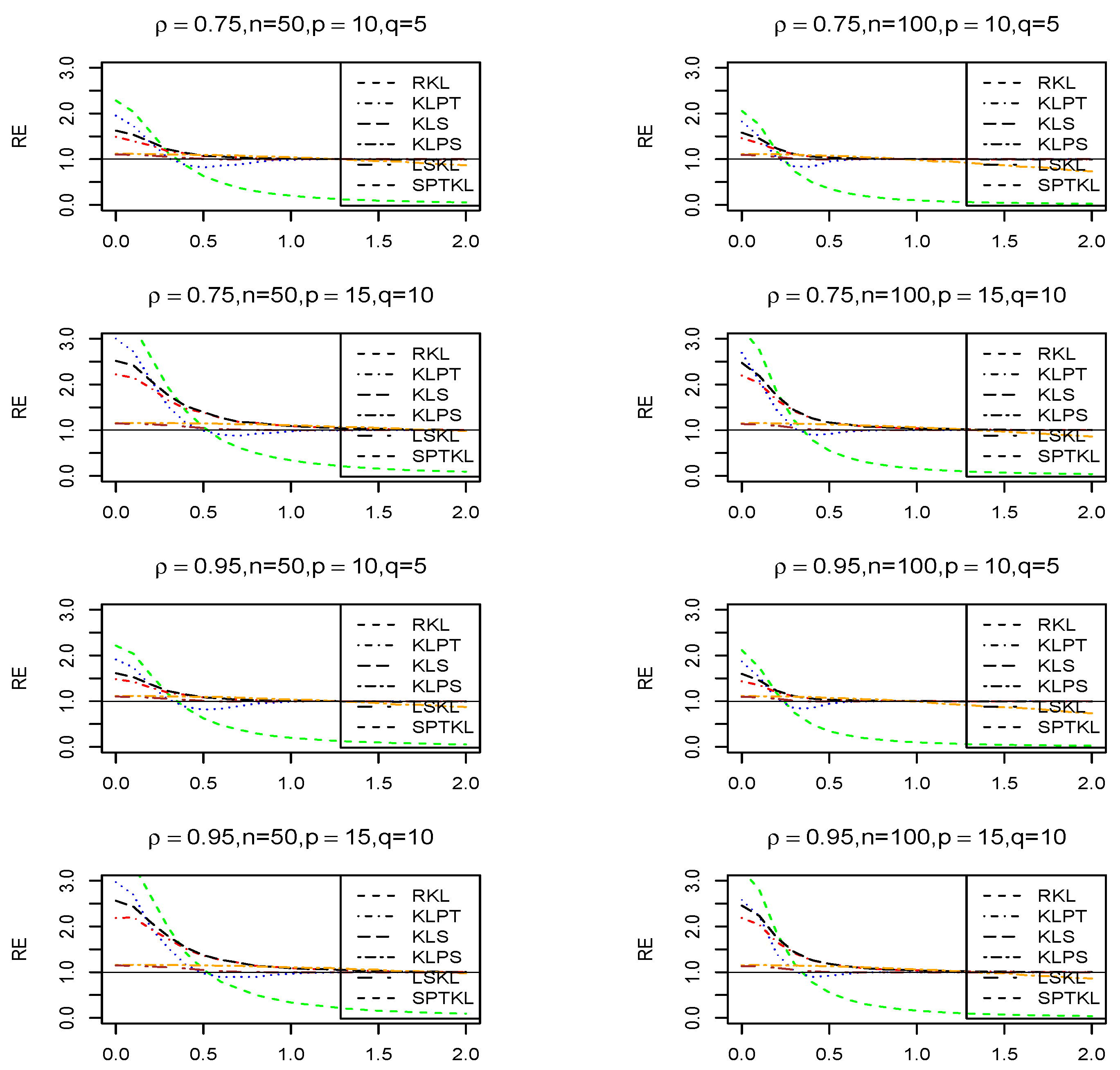
Figure 2.
Correlation Matrix Plot for the Data.
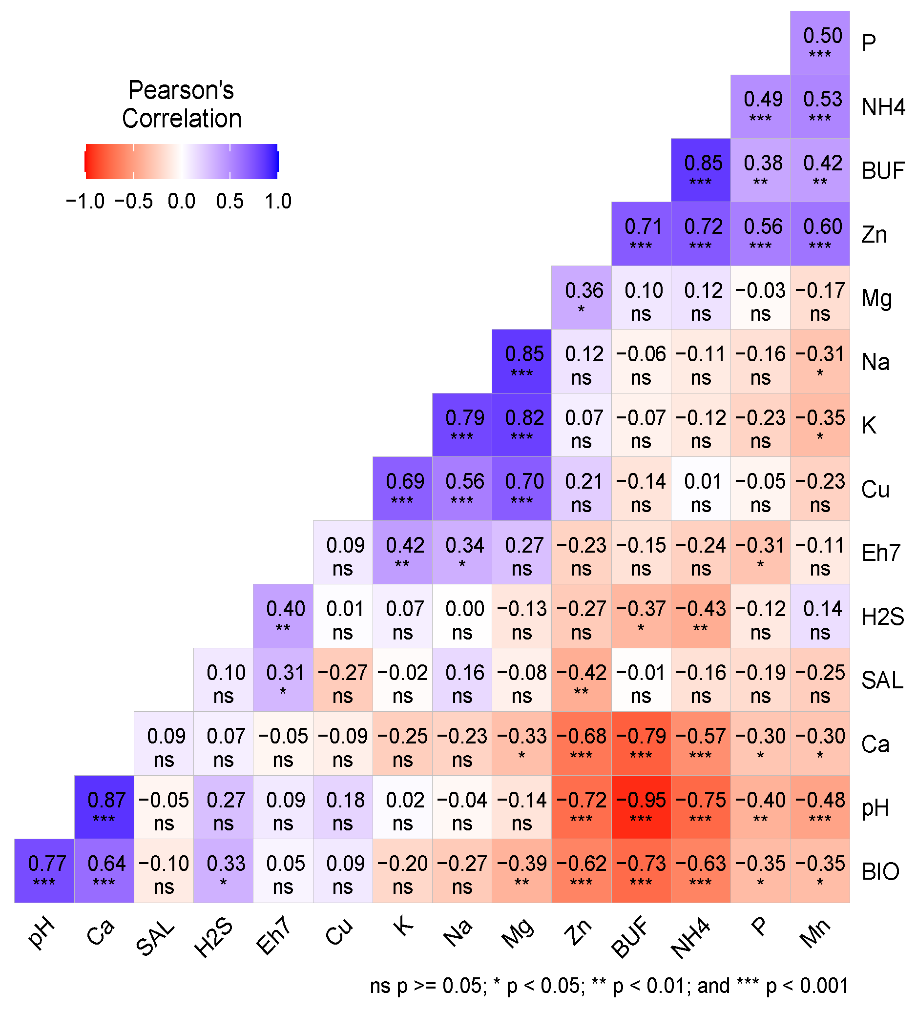
Figure 3.
Variance Inflation factor plot for the data.
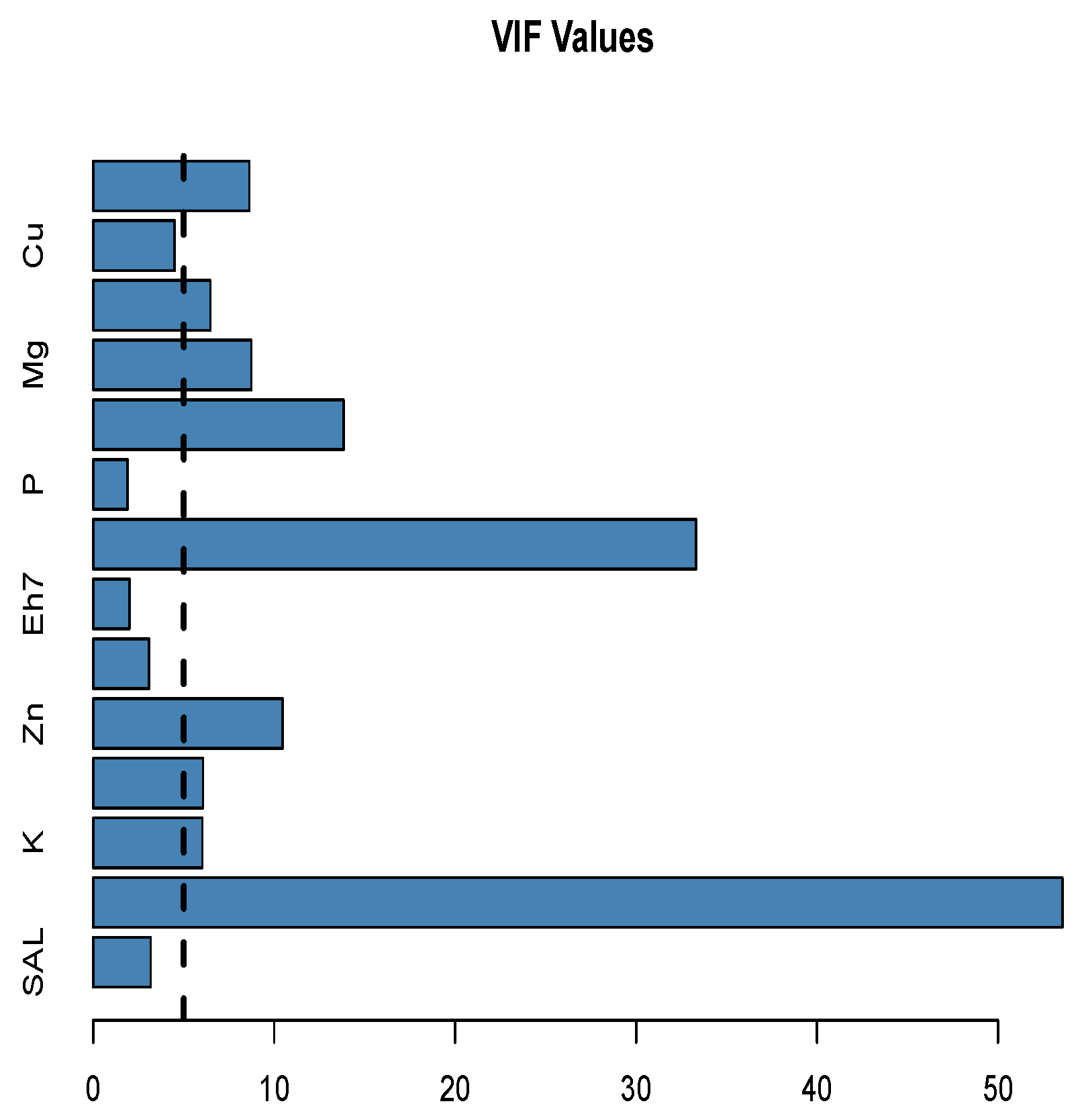
Figure 4.
Box plots of the prediction error for all estimators and algorithms.
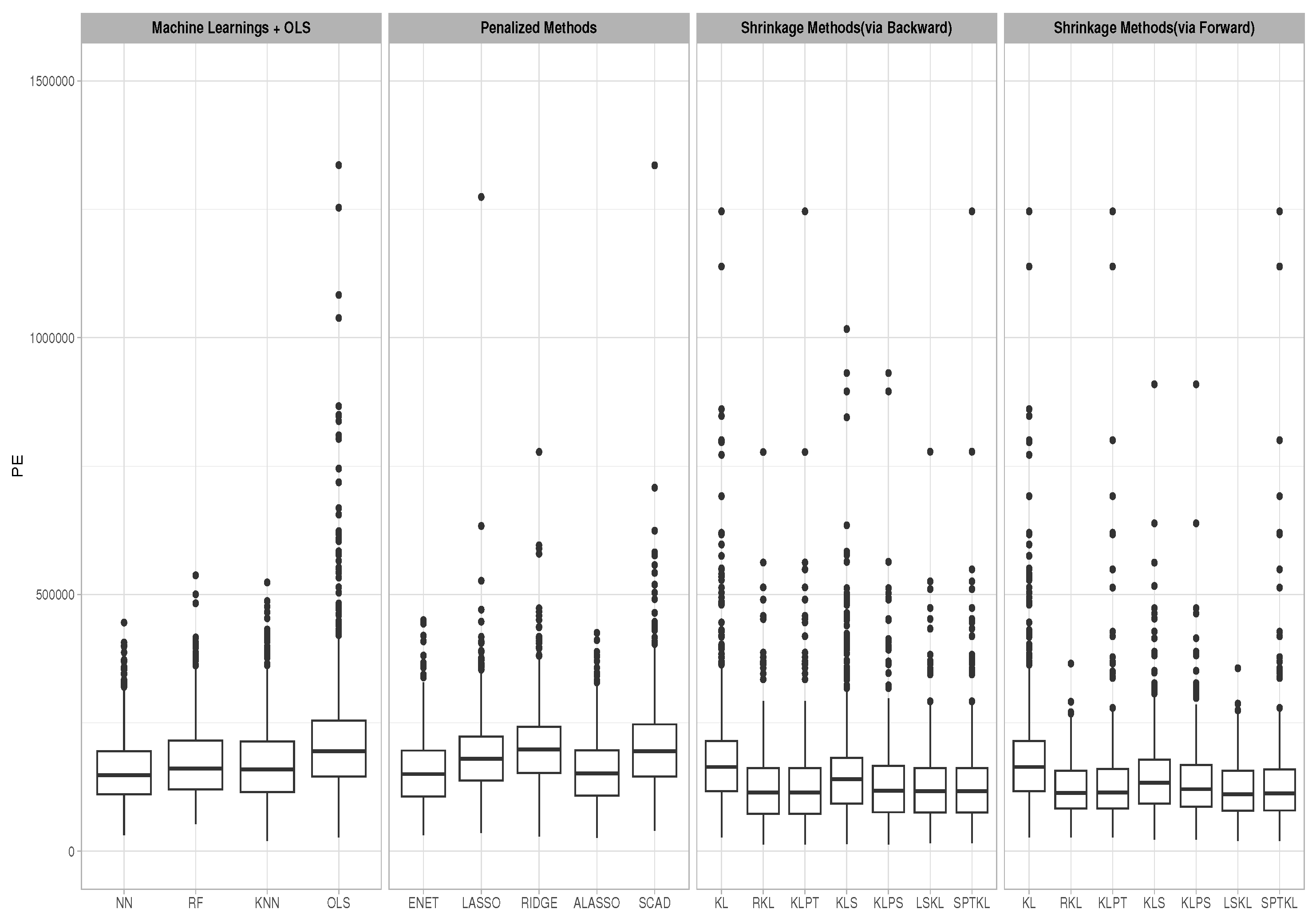

Table 1.
Full and sub models for the data.
| Full Model | FW | BW/BS | Lasso | ALasso | SCAD | ELNT |
| SAL | ✓ | ✓ | ||||
| pH | ✓ | ✓ | ✓ | ✓ | ✓ | |
| K | ✓ | ✓ | ||||
| Na | ||||||
| Zn | ✓ | ✓ | ||||
| H2S | ✓ | ✓ | ||||
| Eh7 | ✓ | ✓ | ✓ | |||
| BUF | ✓ | ✓ | ||||
| P | ✓ | ✓ | ||||
| Ca | ✓ | ✓ | ||||
| Mg | ✓ | ✓ | ✓ | ✓ | ✓ | ✓ |
| Mn | ✓ | |||||
| Cu | ✓ | ✓ | ✓ | ✓ | ✓ | ✓ |
| NH4 | ✓ | ✓ | ✓ | ✓ |
Table 2.
The Relative efficiency of the prediction error for RE-Shrinkage estimators.
| Estimator | Sub.1 | Sub.2 |
| 1.000 | 1.000 | |
| 1.482 | 1.473 | |
| 1.392 | 1.451 | |
| 1.263 | 1.129 | |
| 1.355 | 1.404 | |
| 1.517 | 1.453 | |
| 1.422 | 1.431 |
Table 3.
Relative efficiency of the prediction error for penalized and Machine learning algorithms(MLM).
Table 3.
Relative efficiency of the prediction error for penalized and Machine learning algorithms(MLM).
| Penalized Method | MLM | ||
| Ridge | 0.891 | RF | 1.039 |
| Lasso | 0.983 | KNN | 1.053 |
| ELNT | 1.170 | NN | 1.138 |
| SCAD | 0.889 | ||
| Alasso | 1.148 |
Disclaimer/Publisher’s Note: The statements, opinions and data contained in all publications are solely those of the individual author(s) and contributor(s) and not of MDPI and/or the editor(s). MDPI and/or the editor(s) disclaim responsibility for any injury to people or property resulting from any ideas, methods, instructions or products referred to in the content. |
© 2025 by the authors. Licensee MDPI, Basel, Switzerland. This article is an open access article distributed under the terms and conditions of the Creative Commons Attribution (CC BY) license (http://creativecommons.org/licenses/by/4.0/).
Copyright: This open access article is published under a Creative Commons CC BY 4.0 license, which permit the free download, distribution, and reuse, provided that the author and preprint are cited in any reuse.


