
Submitted:
29 October 2025
Posted:
30 October 2025
You are already at the latest version
Abstract
Multicollinearity and outliers are common challenges in multiple linear regression, often adversely affecting the properties of least squares estimators. To address these issues, several robust estimators have been developed to handle multicollinearity and outliers individually or simultaneously. More recently, [35] introduced the robust Stein estimator (RSE), which integrates shrinkage and robustness to effectively mitigate the impact of both multicollinearity and outliers. Despite its theoretical advantages, the finite-sample performance of this approach under multicollinearity and outliers remains underexplored. Firstly, outliers in the y direction have been the main focus of earlier research on the RSE, not considering outliers in the x direction could substantially impact regression results. This study addresses this gap by considering outliers in both the y and x directions, providing a more thorough assessment of RSE robustness. Lastly, to extend the limited existing benchmark, we compare and evaluate the RSE performance with a wide range of robust and classical estimators. This extends existing benchmarking, which is limited in the current literature. Several Monte Carlo (MC) simulations were conducted, considering both normal and heavy-tailed error distributions, with sample sizes, multicollinearity levels, and outlier proportions varied. Performance was evaluated using bootstrap estimates of root mean squared error (RMSE) and bias. The MC simulation results indicated that the RSE outperformed other estimators under several scenarios where both multicollinearity and outliers are present. Finally, real data studies confirm the MC simulation results.
Keywords:
Robust Stein
; outliers
; multicollinearity
; linear regression
; ordinary least squares
1. Introduction
Linear regression analysis is an important statistical tool that helps to model a relationship between the response variable () and the predictors (), and it is often applied in all fields of study. A linear model has the form
where is an vector of observed values of the dependent variable, is an matrix with a row vector of components of the regressors, , is a vector of unknown parameters and is an vector of errors. Under classical assumptions that the errors have zero mean, constant variance, and are uncorrelated, then the ordinary least-squares (OLS) estimate is the best linear unbiased estimator (BLUE) of according to the Gauss-Markov theorem. The OLS estimate is BLUE even without assuming normally distributed residuals, and minimizes the sum of squared residuals. If an error term () follows a normal distribution, this assumption of normality is essential for performing hypothesis tests and constructing confidence intervals. If there is more than one predictor variable, then the analysis is referred to as multiple linear regression analysis [2]. A multiple regression model could be used to describe this relationship is
Applying the ordinary least squares estimator (OLSE) in simple or multiple linear regression always requires some assumptions, that is, normality of the error terms, equal variance of the error terms, absence of outliers, leverage points, and multicollinearity. Therefore, the OLS estimate is the best method in regression analysis if the assumptions are met. However, if these assumptions are not satisfied, the results can easily be affected [3].
Various problems can occur in the estimation of the model parameters, one of which is if the assumption of normality is not fulfilled, or due to outliers in the data [4]. According to [5,6], the normality of error distributions is based on the central limit theorem, which is a limit theorem based on approximations. Hampel and Huber [5] critically challenged the prevailing assumption that the OLSE remains approximately optimal under conditions of approximate normality. This is because it has been shown that typical error distributions of real-world datasets usually deviate slightly from normality and, in most cases, are tailed. Additionally, outliers in the dependent variable lead to large residual values, which further result in the failure of the normality assumption of the error terms. According to [7], the data that come from the regression line is an outlier. Outliers are data that have different characteristics from other non-outlier data. There exist several statistical methods used to detect outliers, such as the Cook distance index plot and the potential residual plot (see, for example, [8]). The existence of outliers can affect the process of data analysis and errors in making conclusions, but the existence of outliers can be overcome by several methods, which include robust regression [9]. Several robust regression estimators have been provided to address the problem of outliers in different regression models; these include the Huber maximum estimator (HME), the modified maximum likelihood estimator (MME), the least trimmed squares estimator (LTSE), the least median of squares estimator (LMSE), S estimator (SE) [10].
In addition, multicollinearity is another pressing challenge in linear regression models that occurs when predictor variables have a high degree of correlation. This problem causes maximum likelihood estimates to be unstable and inefficient. Therefore, many biased estimators have been provided to address this problem in different regression models [11,12]. However, both multicollinearity and outliers can exist simultaneously in a model. To address both issues, various estimators have been combined for robust estimation in order to handle multicollinearity and outliers [1,13,14]. Recently, the Stein estimator has gained popularity as an alternative to OLSE and performs well in handling correlated regressors. However, it is sensitive to outliers in the y-direction [1]. In this study, we examine a robust version of the Stein estimator, which is the combination of the HME and the James-Stein estimator (JSE), which was originally proposed by [1] and can handle both multicollinearity and outliers simultaneously. This estimator’s performance is assessed and compared with that of other robust regression methods utilizing different simulation scenarios and real data applications.
2. Materials and Methods
In this section, attention will be on the robust methods considered in this study and their properties. The selected estimators were chosen for their theoretical significance as well as their easy implementation and computational viability due to their availability in R. Effective analysis is possible without adding a great deal of computational complexity by using these traditional methods. Because these estimators are available in R, the study is more accessible and reproducible, which makes it useful for other researchers. This decision guarantees an effective combination of computational effectiveness and strong statistical characteristics.
2.1. Review on Robust Estimators
When the data are contaminated by one or a few outliers, the issue of detecting such observations becomes challenging. In general, however, datasets often contain multiple outliers or clusters of influential observations, and they may also exhibit multicollinearity among their variables. These two factors provide additional insight into the co-occurrence of both outliers and multicollinearity, which complicates regression analysis, with biased and unstable parameter estimates as a common result. Alma [15] points out that robust estimation is an important method for analyzing data contaminated by outliers. It is an approach to regression analysis that aims to get past some of the limitations of classical parametric and nonparametric approaches. Well-performing estimates are robust estimates designed to become less sensitive to outliers. Here, we present a review of existing robust estimators used in linear regression.
2.1.1. The Huber Maximum Likelihood Estimator (HME)
The most common general robust method is M-estimates, introduced by [6]. The M in M- estimates stands for maximum likelihood type. The M-estimator minimizes the objective function.
where are called scaled residuals. Differentiating with respect to , assuming is fixed, and setting the partial derivatives to zero, we obtain the normal
equations
Let denote the design matrix, where is the intercept column and contains the p predictors. The ith observation can be written as , where (observations) and (predictors). We consider the spectral decomposition .
2.1.2. James Stein Estimator (JSE)
As a remedy to the problem of multicollinearity, the James-Stein estimator (JSE), originally proposed by [16] and [17], applies shrinkage to the ordinary least squares estimator to improve estimation efficiency under correlated regressors. In the standard regression context, the JSE is given by
where is the ordinary least squares estimator and is the estimated error variance.
In the transformed -space defined in Eq. (5), following [1], the JSE can be expressed as
where the shrinkage factor c is given by
The equivalence between the two forms in Eq. (10) follows from the spectral decomposition, noting that and the canonical transformation diagonalizes the covariance structure into independent components along the eigenvector directions.
2.1.3. The Robust Stein Estimator (RSE)
The robust Stein estimator was first introduced by [1] as an alternative method to the Stein and ridge estimators to improve the accuracy of the estimation. However, both methods are non-robust to outliers. In the author’s study, it was indicated that the Stein estimator is sensitive to outliers in the y-direction. Thus, there is a need to propose the robust Stein estimator [1], which is defined as follows
where, is the M-estimate of , The shrinkage factor in the Robust Stein (M–Stein) estimator is often defined using the following components
where,
- are the ordered eigenvalues of the design information matrix (e.g., in linear models),
- are the components of the robust estimator ,
- are the diagonal entries of the variance-covariance matrix .
The robust covariance matrix is estimated using the sandwich estimator [6]
and is a robust scale estimate. The approximate covariance of is
The approximate bias is
The matrix mean squared error (MMSE) is approximately
The scalar mean squared error (SMSE) is approximately
which can also be expressed as
2.1.4. The Least Median of Squares Estimator (LMSE)
Since M-estimators are not robust to high-leverage outliers, we want to find some methods that can have high BP. [18] defined the least median of squares (LMS) estimator as
which replaces the sum by the median in the LSE.
2.1.5. The Least Trimmed Squares Estimator (LTSE)
Another regression estimator that has a breakdown point (BP) of nearly 50% is the least trimmed square (LTS) estimator proposed by [19]. Traditional OLS methods are highly sensitive to outliers, meaning a few extreme data points can dramatically affect the estimated model. LTSE is designed to be more robust to these outliers by focusing on a subset of the data with the smallest residuals. The estimator chooses the regression coefficients to minimize the sum of the smallest h of the squared residuals and is defined as
where, represents the i-th ordered squared residuals and h is called the trimming constant which must satisfy . The constant h determines the BP of the LTS estimator. Typically, can attain the maximum, where denotes the floor function (rounding down to the next smallest integer). When , LTS is exactly equivalent to the LS estimator whose BP is zero.
2.1.6. The S-Estimator (SE)
To find a simple high-breakdown regression estimator that shares the flexibility and nice asymptotic properties of the M-estimator, [20] introduced the S-estimate. The SE was developed as a robust alternative to traditional estimators like OLSE, particularly when dealing with data containing outliers or high-leverage points. They called it the S-estimate because it is derived from the M-scale estimate equation
In M-estimates, when is unknown, we use Eq. (21) to obtain the scale parameter and regression estimates simultaneously. Let , where represents the standard normal density, and let
When (where a is the upper bound of and ), the scale has a unique positive solution. If , it may have infinite solutions including , and if , then no solution exists.
To avoid such indeterminacies, we define that whenever , we set .
To define the S-estimator, we let satisfy the following condition
- (A1)
- is symmetric, continuously differentiable, and ;
- (A1)
- There exists such that is strictly increasing on and constant on .
For each vector , using Eq (21), we can calculate the dispersion of residuals , where satisfies (A1). Then the S-estimator is defined by
2.1.7. The Modified Maximum Likelihood Estimator (MME)
The MM estimation is a special type of M-estimation developed by [21], and is particularly useful when dealing with non-normal data or outliers. MM estimation is a combination of high breakdown value estimation and efficient estimation. MM estimator was the first estimator with both a high breakdown point and high efficiency under normal error. The MM-estimator follows a three-stage procedure
Stage 1:
Compute an initial consistent robust estimate with high breakdown point (BP), possibly 50%, but not necessarily efficient.
Stage 2:
Stage 3:
Let be another -function satisfying (A1) such that
and
Let and define the objective function
Then the MM-estimate is defined as any solution to
that also satisfies
Yohai [21] showed that any value of satisfying Eq. (26) and (27), for example a local minimum, will have the same efficiency as the global minimum, and its BP is no less than that of . Thus, although the absolute minimum of exists, it is not necessary to find it.
In the first stage, the robust initial estimate should satisfy regression, scale, and affine equivariance and have a high BP. LMS, LTS, and S-estimates are possible candidates.
For Stage 2, one way of choosing and is as follows: Let be a function satisfying (A1), and define
In order to satisfy Eq. (23), we must have . The value of should be chosen such that holds.
2.2. Criteria for Assessing the Estimator’s Performance
Following a study by [23], two typical measures of accuracy for the estimator are the RMSE and the Bias. These measures can be estimated using bootstrap resampling. Specifically, given B bootstrap samples, the bootstrap estimate of Bias and RMSE is as follows
2.2.1. Bias Under the Bootstrap
where are bootstrap copies of .
2.2.2. RMSE Under the Bootstrap
3. Monte Carlo Simulation Study
3.1. Simulation Procedure
The data generation process that follows was adapted from [24] and [25]. We generate n samples from the model using R studio
where the error terms are generated as , and the explanatory variables are generated using the following equation
where are independent standard normal random numbers that are held fixed for a given sample of size n, and is the degree of multicollinearity between predictors. In this study, we consider three values of = 0.10, 0.50, and 0.98. The past study [1] mainly examined the RSE under high correlation; we extend the analysis to low and moderate levels to better understand its performance across varying degrees of multicollinearity.
The true values of the regression parameters are chosen as , which is a common restriction in simulation studies (see, for example, [1,13] and [26]). Additionally, the performance of the RSE is also evaluated for heavy-tailed error distributions, such as t-distributions and the Cauchy distribution.
Five different sample sizes are considered , with the number of predictors fixed at , and different proportions of outliers are evaluated . In each simulation setting, we perform MC replications, which is chosen as a compromise between achieving a low MC error and keeping the computation time reasonable.
To introduce outliers in the data, we consider two types, that is, y direction outliers and x direction outliers. For y direction outliers, we first generate the clean data according to equations (30) and (31) then randomly select observations and replace their response values by adding a large constant, that is, , where is the standard deviation of the error term. For x direction outliers, we randomly select observations and replace their predictor values with , where is the standard deviation of the j-th predictor.
A summary of the simulation scenarios is provided in Table 1. In addition, we evaluate the performance of the proposed estimators under the following ten cases
- Case I: - Standard normal distribution with 0.10, 0.50, and 0.98 multicollinearity and 0.00% outliers.
- Case II: — Student’s t-distribution with 7 degrees of freedom with 0.10, 0.50, and 0.98 multicollinearity and 0.00% outliers.
- Case III: — Student’s t-distribution with 2 degrees of freedom, 0.10, 0.50, and 0.98 multicollinearity and 0.00% outliers.
- Case IV: — Cauchy distribution errors with 0.10, 0.50, and 0.98 multicollinearity and 0.00% outliers.
- Case V: — Standard normal distribution with 10%, 25%, and 50% outliers with no multicollinearity.
- Case VI: — Student’s t-distribution with 2 degrees of freedom, 10%, 25%, and 50% outliers with no multicollinearity.
- Case VII: — 10%, 25%, and 50% outliers in the y-direction with 0.10, 0.50, and 0.98 multicollinearity.
- Case VIII: — 10%, 25%, and 50% outliers in the x-direction with 0.10, 0.50, and 0.98 multicollinearity.
- Case IX: (Student’s t-distribution with 2 degrees of freedom), with multicollinearity levels of 0.10, 0.50, and 0.98, and outliers in the y-direction at 10%, 25%, and 50%.
- Case X: (Student’s t-distribution with 2 degrees of freedom), with multicollinearity levels of 0.10, 0.50, and 0.98, and outliers in the x-direction at 10%, 25%, and 50%.

Table 1.
Summary of Simulation Parameters Considered.
| Sample size (n) | Multicollinearity () | Outlier () |
|---|---|---|
| 25 | 0.10 | 0.00 |
| 50 | 0.50 | 0.10 |
| 100 | 0.98 | 0.25 |
| 150 | 0.50 | |
| 200 |
3.2. Simulation Study Findings
3.2.1. Performance Evaluation Findings Across the Cases
Case I (Table A3 and Figure 1): The JSE and RSE yield the smallest RMSE values across all sample sizes, consistent with their theoretical optimality properties. The MME, HME, OLSE, and LTSE also achieve RMSE values comparable to those of JSE and RSE only when = 0.50 and 0.98. In contrast, the LMSE and SE display relatively higher RMSEs, reflecting their lower efficiency in the presence of multicollinearity. The JSE and RSE have achieved exactly zero bias for low multicollinearity = 0.10 and 0.50 at sample sizes at , and LMSE shows the highest bias across nearly all scenarios. All estimators exhibit monotonic behavior, with RMSE values consistently decreasing as the sample size increases.
Case II (Table A4, and Figure 2): The RSE consistently achieves the lowest RMSE across all the conditions in this case. The JSE consistently achieves low bias across different sample sizes and multicollinearity levels. The LMSE has the overall worst performance across all the simulation scenarios.
Case III (Table A5 and Figure 3): In this case, the performance of the OLSE, JSE, and LMSE is substantially worse than that of any other robust estimators. The RSE, MME, and HME exhibit RMSE values that are almost similar, but the RSE is outperforming all the estimators in this case, as shown in Figure 3. The HME and MME consistently achieve low bias in almost all sample sizes and multicollinearity levels, and JSE has the highest bias at = 0.50 and 0.98.
Case IV(Table A6, and Figure 4): Under Cauchy-distributed errors, OLSE and JSE demonstrate erratic RMSE behavior, with values escalating due to the heavy-tailed nature of the distribution. In contrast, robust estimators maintain lower RMSEs and a monotonic decrease with increasing sample size, highlighting their stability. Furthermore, as the correlation coefficient () increases, the performance of OLSE and JSE worsens further. The RSE is the best estimator under the Cauchy distribution as shown by Figure 4. HME and MME continue to maintain a consistently lowest bias across all scenarios at = 0.98 and n = 200. OLSE and JSE are having the highest bias with values exceeding one.
Case V (Table A7, Table A8, and Figure 5, Figure 6): The MME performs the best under y direction, and LTSE performs the best under x direction. RSE yields a higher RMSE because it lacks robustness in both x and y directions. LTSE and SE maintain a small bias and low RMSE in the presence of x-outliers, whereas RSE, JSE, and OLSE break down due to high sensitivity, as shown in Figure 5 and Figure 6.
Case VI (Table A9, Table A10, and Figure 7, Figure 8):Table A9 and Figure 7 show that the MME, SE, HME, and LTSE consistently achieve the lowest RMSE and almost zero bias, making it the best performers, while the RSE, OLSE, and JSE perform the worst due to high RMSE values. Table A10 and Figure 8 indicate that the LTSE, MME, and SE are the most robust and accurate, while the RSE and JSE again show the poorest performance.
Case VII (Table A11, Table A12, Table A13, and Figure 9, Figure 10, Figure 11): When the data contains multicollinearity and outliers in the response direction, the performance of the OLSE, JSE, and LMSE worsens significantly, particularly as the percentage of outliers and the degree of multicollinearity increase as shown by Figure 9, Figure 10, and Figure 11. The following estimators, the LMSE, OLSE, and JSE in Figure 11, completely fail when 50% of the observations are contaminated. In contrast, the RSE, SE, HME, and MME demonstrate superior performance relative to OLSE, JSE, and LMSE under the same conditions. Moreover, the LTSE and SE exhibit even better robustness, maintaining substantially lower RMSE values compared to OLSE, JSE, and LMSE, particularly in the presence of low contamination, which is 10% in Figure 9. When there are 25% of outliers in Figure 10, we observe similar patterns with Figure 9. The RSE performs very well in cases of outliers and multicollinearity, followed by MME, HME, and LTSE.
Case VIII (Table A14, Table A15, Table A16, and Figure 12, Figure 13, Figure 14): The RSE is outperforming all the estimators in all scenarios when the data contains multicollinearity and the outliers in the x direction. The performance of LMSE, SE, LTSE, and OLSE worsens significantly as the percentage of outliers and multicollinearity increases, as shown by Figure 12, Figure 13, Figure 14. The bias is the smallest for SE and MME when and 50%.
Cases IX (Table A17, Table A18, Table A19, and Figure 15, Figure 16, Figure 17): The RSE consistently performs better than average performance among all the simulation scenarios. When 10% outliers and multicollinearity are present, the HME, MME, LTSE, and SE work with similar results as shown in Figure 15. The JSE and OLSE, in contrast, always give the poorest performance in all of these scenarios. LMSE shows less than ideal accuracy of performance as well, specifically under 10% contamination, over which it generates the largest bias values. Overall, the HME and MME are the most accurate estimators, with consistently lower bias compared to other methods.
Cases X (Table A20, Table A21, Table A22, and Figure 18, Figure 19, Figure 20): RMSE values are shown in Figure 18, Figure 19 and Figure 20 under different multicollinearity and x-outlier levels. The RMSE increases with both higher multicollinearity and larger proportions of x-outliers. RSE consistently provides the lowest RMSE, reflecting good stability, while OLSE and JSE perform the worst. In terms of bias, HME and MME both show the lowest bias in all scenarios, and JSE shows the highest bias. These findings also emphasize the better performance of RSE, and therefore its robustness and accuracy, and show the relative bias performance of the other estimators under challenging data conditions.
In summary, JSE and OLSE only work well when there are no outliers since it is very sensitive to outliers. The estimator’s bias and RMSE values were increased in the case of the multicollinearity degree () and outlier percentage (), and decreased in the case of the sample size (n) being increased, when other factors were fixed. When only the multicollinearity problem existed in the model (as in Figure 1 and Figure 2, or when no outliers existed, i.e., ), the OLSE, JSE, HME, MME, and RSE were better than LMSE, LTSE, and SE. But in Figure 4, OLSE and JSE performed the worst, even though they had no outliers. When both problems existed (as in Figure 9, Figure 10, Figure 11, Figure 12, Figure 13, and Figure 14 or when outliers existed, i.e., ), the RSE, HME, and MME were better than the LMSE, LTSE, SE, JSE, and OLSE, respectively, for all , , and n values. Finally, the RSE achieved the best performance among all given estimators when outliers and multicollinearity exist.
4. Emprical Applications
In the previous section, we conducted an MC simulation study to compare the performance of the estimators. However, simulations are usually performed under some ideal conditions. In contrast to the MC simulation, this section considers three real linear regression datasets as an illustrative example in handling outliers and multicollinearity in linear regression. The datasets are the Milk dataset, the Real Estate Valuation dataset, and the Hawkins–Bradu–Kass dataset. We adopted a systematic trimming procedure in accordance with [27] to modify the outlier contamination levels in each dataset because real datasets frequently contain variable and uncontrollable levels of outliers. A direct comparison of theoretical, simulated, and real-data results is made possible by this method, which enables us to produce multiple versions of each dataset with particular outlier percentages that match our simulation study design. A summary of the datasets considered for this study is provided in Table A1.
Study 1: Milk Dataset
Milk dataset provided [28] is a composition of milk with 8 variables. The 8 variables are density, fat content, protein content, casein content, cheese dry substance measured in the factory, cheese dry substance measured in the laboratory, milk dry substance, and cheese produced. According to [28], the are 17 outliers in this dataset, which makes the percentage of outliers 20%. Observations (1st–3rd, 12th, 13th–17th, 27th, 41st, 44th, 47th, 70th, 74th, 75th and 77th) are outliers.
4.1. Exploratory Analysis for Milk Dataset
4.1.1. Multicollinearity Detection for Milk Dataset
Table A2 presents VIF for milk dataset, which is a crucial diagnostic tool for detecting multicollinearity in regression analysis. The VIF quantifies how much the variance of a regression coefficient increases due to collinearity with other predictor variables. A VIF value greater than 10 indicates high multicollinearity. It is noted that from the milk dataset, variables and exhibit high VIF. Moreover, the observed condition number (CN) of 164.0314 indicates that strong multicollinearity exists among the regressors. It is observed from the Table 2 that some regressors (,,,) are highly correlated.
4.1.2. Outlier Detection Using Cook’s Distance for Milk Dataset
The Cook’s distance plot for the Milk dataset, with a threshold value of 0.047, is displayed in Figure 21. It was discovered that two observations (70 and 74) greatly surpass this threshold, with observation 70 achieving a value above 2.0. These data points are considered to be very significant and deserving of more investigation. Their existence indicates the possibility of anomalies or leverage points that might influence model predictions.
4.1.3. Testing for Normality for Milk Dataset
For this study, both theoretical and graphical techniques will be used to assess the normality of the OLS residuals. The Shapiro-Wilk (SW) test will be used as a theoretical tool. Figure 22 shows a diagnostic plot to assess residual normality in milk data. Visual inspection of these plots reveals that the Milk data displays approximately normal residuals. The results of the theoretical test yielded a p-value of 0.1964 (), indicating that the milk data follows a normal distribution.
4.1.4. Model Fit and Evaluation for Milk Dataset
To compare the performance of the methods, the regression model was fitted using the Milk dataset for each method, considering the sparsity of the models. The bias and RMSE were finally used to evaluate how well the methods performed. The results presented in Table 3 cover the bias and the RMSE of each estimation method for the Milk dataset. The results show that the RSE has outperformed all the estimates when there are both outliers and multicollinearity. When there is multicollinearity and 0% outliers, the JSE, OLSE, and other robust estimates have almost the same RMSE values, the same thing that was happening in our simulation study in chapter four. The next estimators with similar performance when multicollinearity and outliers exist are JSE, MME, and HME. Figure 23 was used to assess the bias and RMSE. It was observed that the OLSE bias (red line) increases with increasing outlier percentage. The RSE RMSE values (black line) decrease with increasing outlier percentage.
Study 2 : Real Estate Valuation Dataset
Real estate valuation was collected in 2018 from Sindian District, New Taipei City, Taiwan, and it was recently published by [29]. The response variable in this study is the house price of unit area, measured in 10,000 New Taiwan Dollars per Ping, where one Ping corresponds to . The explanatory variables include the transaction date (), the house age in years (), the distance to the nearest MRT station in meters (), the number of convenience stores within walking distance (), the geographic coordinate latitude in degrees (), and the geographic coordinate longitude in degrees ().
4.2. Exploratory Analysis for Real Estate Valuation
4.2.1. Multicollinearity Detection for Real Estate Valuation
4.2.2. Outlier Detection Using Cook’s Distance for Real Estate Valuation Dataset
Figure 24 displays the Cook’s distance plot with a 0.01 threshold for the real estate valuation dataset. In comparison to the other points, observation 271 shows a significantly higher Cook’s D value, indicating a significant impact on the regression results. Data points 149, 221, and 313 show additional moderate influences.
4.2.3. Testing for Normality for Real Estate Valuation Dataset
Figure 25 shows clear departures from normality due to skewed residual distributions. Therefore, the theoretical test confirms that the data is not normally distributed as the p-value is less than 0.05 ().
4.2.4. Model Fit and Evaluation for eal Estate Valuation Dataset
Table 5 presents the estimated bias and RMSE of various estimators under increasing levels of outlier contamination and multicollinearity. The RSE demonstrates the most consistent performance in terms of RMSE across all contamination levels, particularly excelling at higher outlier percentages. While JSE shows the lowest RMSE under clean data, its performance deteriorates significantly with more outliers. HME and OLSE maintain relatively low bias at all levels, but often at the cost of higher RMSE. Figure 26 was used to assess bias and RMSE. It was observed that HME, OLSE, and RSE maintain consistently low bias across all outlier levels. The RSE and JSE are the clear top performers with the low RMSE values. Despite the fact that RSE outperforms all other estimators in terms of RMSE, it exhibits higher bias compared to some of them. This indicates that while RSE achieves the best overall predictive accuracy by effectively balancing bias and variance, it does not perform best in terms of bias alone. Therefore, the RSE is the most outperforming estimator as outlier percentage increases, suggesting it has strong abilities to detect and manage multicollinearity and outliers.
4.3. Exploratory Analysis for Hawkins Bradu Kass Dataset
4.3.1. Multicollinearity Detection for Hawkins Bradu Kass Dataset
It is noteworthy that all predictors exhibit exceptionally high VIF values in Hawkins Bradu Kass dataset as shown in Table A2, and the observed CN of 102.5294 indicates that strong multicollinearity exists among the regressors. It is observed from the Table 6 that some regressors (,) are highly correlated.
4.3.2. Outlier Detection Using Cook’s Distance for Hawkins Bradu Kass Dataset
The Cook’s distance plot for the Hawkins Bradu Kass dataset, with a threshold value of 0.053, is displayed in Figure 27. Cook’s D values in observations 12 and 14 significantly surpass the threshold, highlighting the fact that they are as highly significant outliers. If not appropriately addressed, these points might bias the parameter estimates and overall model performance.
4.3.3. Testing for Normality for Hawkins Bradu Kass Dataset
Figure 28 shows clear departures from normality due to skewed residual distributions. Therefore, the theoretical test confirms that the data is not normally distributed as the p-value is less than 0.05 ().
4.3.4. Model Fit and Evaluation for Hawkins Bradu Kass Dataset.
As shown in Table 7 and Figure 29, in the absence of outliers, the JSE achieved the lowest RMSE, while HME had the lowest bias. Under 18.67% outlier contamination with multicollinearity, SE produced the lowest bias, and RSE achieved the lowest RMSE. MME also performed well under contamination, demonstrating both low bias and RMSE. In contrast, OLSE experienced a significant increase in both bias and RMSE when exposed to outliers. Overall, robust estimators like RSE and MME display greater stability and resilience under data contamination.
5. Discussion
The outcomes are consistent with the current literature regarding robust regression estimators. RSE’s superior performance in the presence of simultaneous multicollinearity and outlier contamination is attributed to its dual-component structure, that is, the HME component reduces the influence of outliers, while the JSE component maintains estimates through shrinkage, thereby alleviating variance inflation [1].
The MME performed better when outliers only appeared in the y-direction and there was no multicollinearity. This pattern is consistent with the findings of [30] and [31], who found that MME was the most effective estimator for pure vertical contamination. The failure of OLSE and JSE in the presence of Cauchy-distributed errors corroborates the conclusions of [32] and [33], which indicate that heavy-tailed distributions lead to extreme observations dominating the sum of squared residuals. One basic trade-off in robust estimation is demonstrated by the failure of high-breakdown estimators (LMSE, LTSE, SE) under multicollinearity without outliers [20]. This study’s overall findings support the idea that no single estimator is always the best. MME maintains advantages in environments dominated by y-direction outliers without multicollinearity [30,31,34], whereas RSE performs best when both multicollinearity and outliers are present [1]. These results highlight how crucial diagnostic analysis is prior to deciding on an estimation technique.
6. Concluding Remarks
This study evaluates the performance of RSE, which combines the shrinkage factors of ME and JSE, in the presence of multicollinearity and outliers in both the x and y directions. We evaluate the efficiency of RSE in an extensive MC simulation study with bias and RMSE criteria. As it stands, the simulation study is performed under several distributional conditions (normally, t-distributions, and Cauchy distributed errors), sample sizes, levels of multicollinearity, and outliers in both the x and y directions separately.
When multicollinearity and outliers in x and y directions exist, the RSE outperforms the classical OLSE, JSE, HME, MME, LMSE, LTSE, and SE. Additionally, when comparing the RSE to other existing robust estimators, we see that in the majority of the simulation scenarios evaluated, the RSE performs better. Based on the simulation study and its application to real datasets, we find that the RSE is the best estimator under conditions of multicollinearity and outliers in both the x and y directions. Future research may extend this work by comparing the RSE through simulation studies using various distributions, such as the Weibull, Gamma, and Poisson distributions, across different sample sizes, levels of outlier contamination, and degrees of multicollinearity.
Author Contributions
Conceptaulization, L.D., C.S.M; methodology, L.D., C.S.M; software, L.D; validation, L.D., C.S.M; formal analysis, L.D; investigation, L.D, C.S.M; resources, L.D; writing original draft preparation, L.D; writing review and editing, L.D., C.S.M, and L.K; visualization, L.D., C.S.M, and L.K; supervisor, C.S.M; project administration, C.S.M. All authors have read and agreed to the published version of the manuscript.
Funding
This research was supported by a fee waiver bursary from the University’s Research and Innovation Office, which also contributed partial funding for the article processing charges (APC).
Data Availability Statement
The data used to support the findings of this study are included within the article.
Acknowledgments
The authors would like to express their sincere gratitude to the reviewers and the editor for their insightful comments and constructive feedback, which significantly contributed in improving the quality of this paper.
Conflicts of Interest
The authors declare no conflict of interest.
Appendix A
Appendix A.1
Table A1.
Summary of the Datasets.
| Study No. | Dataset | n | p | No. of Outliers | Outliers (%) |
|---|---|---|---|---|---|
| Milk dataset (original) | 86 | 8 | 20 | 20% | |
| 1 | Milk trimmed dataset | 62 | 8 | 0 | 0% |
| Milk trimmed dataset | 81 | 8 | 8 | 10% | |
| Real Estate Valuation (original) | 414 | 7 | 88 | 21.25% | |
| 2 | Real Estate Valuation trimmed dataset | 212 | 7 | 0 | 0% |
| Real Estate Valuation trimmed dataset | 268 | 7 | 41 | 15.3% | |
| Hawkins–Bradu–Kass dataset (original) | 75 | 4 | 14 | 18.67% | |
| 3 | Hawkins–Bradu–Kass trimmed dataset | 61 | 4 | 0 | 0% |
Table A2.
Variance Inflation Factor (VIF) of Milk Dataset, Real Estate Dataset, and Hawkins Bradu Kass Dataset.
Table A2.
Variance Inflation Factor (VIF) of Milk Dataset, Real Estate Dataset, and Hawkins Bradu Kass Dataset.
| Dataset | Variable | VIF | Variable | VIF |
|---|---|---|---|---|
| Milk dataset | 2.2007 | 24.7561 | ||
| 8.2865 | 3.2919 | |||
| 7.2187 | 2.1834 | |||
| 24.2253 | ||||
| Real Estate Valuation dataset | 1.0147 | 1.6023 | ||
| 1.0143 | 2.9263 | |||
| 4.3230 | ||||
| 1.6170 | ||||
| Hawkins Bradu Kass datase | 13.4320 | |||
| 23.8535 | ||||
| 33.4325 |
Table A3.
Estimated Bias and RMSE Values with Multicollinearity and no Outliers for Normal Distribution .
Table A3.
Estimated Bias and RMSE Values with Multicollinearity and no Outliers for Normal Distribution .
| Method | |||||||
|---|---|---|---|---|---|---|---|
| BIAS | RMSE | BIAS | RMSE | BIAS | RMSE | ||
| OLSE | 25 | 0.0048 | 0.7969 | 0.0071 | 0.5625 | 0.0080 | 2.1962 |
| 50 | 0.0031 | 0.5451 | 0.0064 | 0.3860 | 0.0173 | 1.5106 | |
| 100 | 0.0016 | 0.3808 | 0.0025 | 0.2692 | 0.0096 | 1.0585 | |
| 150 | 0.0019 | 0.3016 | 0.0010 | 0.2140 | 0.0036 | 0.8410 | |
| 200 | 0.0008 | 0.2651 | 0.0014 | 0.1833 | 0.0153 | 0.7204 | |
| HME | 25 | 0.0004 | 0.7367 | 0.0055 | 0.5905 | 0.0193 | 2.3061 |
| 50 | 0.0049 | 0.4955 | 0.0052 | 0.4067 | 0.0173 | 1.5944 | |
| 100 | 0.0021 | 0.3392 | 0.0009 | 0.2817 | 0.0050 | 1.1043 | |
| 150 | 0.0032 | 0.2705 | 0.0029 | 0.2245 | 0.0135 | 0.8834 | |
| 200 | 0.0027 | 0.2369 | 0.0016 | 0.1924 | 0.0152 | 0.7554 | |
| MME | 25 | 0.0048 | 0.7450 | 0.0065 | 0.6064 | 0.0160 | 2.3551 |
| 50 | 0.0034 | 0.4964 | 0.0064 | 0.4113 | 0.0191 | 1.6135 | |
| 100 | 0.0029 | 0.3450 | 0.0010 | 0.2885 | 0.0080 | 1.1326 | |
| 150 | 0.0032 | 0.2735 | 0.0029 | 0.2338 | 0.0181 | 0.9137 | |
| 200 | 0.0033 | 0.2377 | 0.0005 | 0.2031 | 0.0184 | 0.7736 | |
| LMSE | 25 | 0.0236 | 1.5696 | 0.0125 | 1.4520 | 0.0490 | 5.6943 |
| 50 | 0.0144 | 1.1159 | 0.0225 | 1.0589 | 0.0505 | 4.1858 | |
| 100 | 0.0114 | 0.8152 | 0.0045 | 0.8262 | 0.0335 | 3.1939 | |
| 150 | 0.0067 | 0.6859 | 0.0073 | 0.7339 | 0.0387 | 2.7792 | |
| 200 | 0.0087 | 0.6201 | 0.0094 | 0.6494 | 0.0063 | 2.4765 | |
| LTSE | 25 | 0.0076 | 0.9591 | 0.0033 | 0.8883 | 0.0473 | 3.3716 |
| 50 | 0.0038 | 0.5957 | 0.0080 | 0.5332 | 0.0150 | 2.0957 | |
| 100 | 0.0036 | 0.3777 | 0.0057 | 0.3466 | 0.0162 | 1.3443 | |
| 150 | 0.0043 | 0.3010 | 0.0013 | 0.2741 | 0.0124 | 1.0760 | |
| 200 | 0.0027 | 0.2567 | 0.0034 | 0.2336 | 0.0170 | 0.9105 | |
| SE | 25 | 0.0135 | 1.1950 | 0.0122 | 1.1329 | 0.0784 | 4.3873 |
| 50 | 0.0089 | 0.8378 | 0.0082 | 0.8368 | 0.0301 | 3.3277 | |
| 100 | 0.0099 | 0.5921 | 0.0028 | 0.6184 | 0.0254 | 2.3643 | |
| 150 | 0.0071 | 0.4814 | 0.0031 | 0.5198 | 0.0295 | 2.0266 | |
| 200 | 0.0027 | 0.4170 | 0.0037 | 0.4561 | 0.0173 | 1.7737 | |
| JSE | 25 | 0.0037 | 0.2250 | 0.0107 | 0.4773 | 0.0661 | 1.9841 |
| 50 | 0.0003 | 0.0370 | 0.0076 | 0.3276 | 0.0430 | 1.2924 | |
| 100 | 0.0000 | 0.0000 | 0.0046 | 0.2253 | 0.0434 | 0.8524 | |
| 150 | 0.0000 | 0.0000 | 0.0025 | 0.1809 | 0.0256 | 0.6505 | |
| 200 | 0.0000 | 0.0000 | 0.0024 | 0.1535 | 0.0194 | 0.5438 | |
| RSE | 25 | 0.0037 | 0.1838 | 0.0116 | 0.5022 | 0.0759 | 2.0991 |
| 50 | 0.0003 | 0.0235 | 0.0065 | 0.3444 | 0.0461 | 1.3762 | |
| 100 | 0.0000 | 0.0000 | 0.0055 | 0.2366 | 0.0425 | 0.8949 | |
| 150 | 0.0000 | 0.0000 | 0.0033 | 0.1896 | 0.0329 | 0.6874 | |
| 200 | 0.0000 | 0.0000 | 0.0028 | 0.1611 | 0.0233 | 0.5744 | |
Note: OLSE (Ordinary Least Squares Estimator), HME (Huber Maximum Likelihood Estimator), MME (Modified Maximum Likelihood Estimator), LMSE (Least Median of Squares Estimator), and LTSE (Least Trimmed Squares Estimator). SE (S-Estimator), JSE (James–Stein Estimator), and RSE (Robust Stein Estimator).
Table A4.
Estimated Bias and RMSE Values with Multicollinearity and no Outliers for Student’s t-distribution with 7 Degrees of Freedom .
Table A4.
Estimated Bias and RMSE Values with Multicollinearity and no Outliers for Student’s t-distribution with 7 Degrees of Freedom .
| Method | |||||||
|---|---|---|---|---|---|---|---|
| BIAS | RMSE | BIAS | RMSE | BIAS | RMSE | ||
| OLSE | 25 | 0.0123 | 0.7426 | 0.0066 | 0.7806 | 0.0216 | 3.0798 |
| 50 | 0.0027 | 0.4939 | 0.0037 | 0.5268 | 0.0152 | 2.0303 | |
| 100 | 0.0054 | 0.3541 | 0.0062 | 0.3753 | 0.0169 | 1.4894 | |
| 150 | 0.0010 | 0.2870 | 0.0053 | 0.3012 | 0.0153 | 1.1769 | |
| 200 | 0.0058 | 0.2611 | 0.0045 | 0.2817 | 0.0069 | 1.0910 | |
| HME | 25 | 0.0061 | 0.6519 | 0.0154 | 0.6874 | 0.0306 | 2.7191 |
| 50 | 0.0035 | 0.4402 | 0.0072 | 0.4624 | 0.0192 | 1.7788 | |
| 100 | 0.0039 | 0.3065 | 0.0040 | 0.3260 | 0.0102 | 1.2931 | |
| 150 | 0.0018 | 0.2491 | 0.0035 | 0.2613 | 0.0236 | 1.0218 | |
| 200 | 0.0019 | 0.2184 | 0.0017 | 0.2308 | 0.0067 | 0.9018 | |
| MME | 25 | 0.0091 | 0.6554 | 0.0116 | 0.6922 | 0.0222 | 2.7395 |
| 50 | 0.0020 | 0.4447 | 0.0037 | 0.4656 | 0.0166 | 1.7988 | |
| 100 | 0.0051 | 0.3109 | 0.0046 | 0.3317 | 0.0031 | 1.3056 | |
| 150 | 0.0043 | 0.2569 | 0.0053 | 0.2669 | 0.0206 | 1.0457 | |
| 200 | 0.0019 | 0.2233 | 0.0019 | 0.2338 | 0.0051 | 0.9262 | |
| LMSE | 25 | 0.0018 | 1.4606 | 0.0085 | 1.5271 | 0.0909 | 6.0429 |
| 50 | 0.0074 | 1.0703 | 0.0124 | 1.1522 | 0.0852 | 4.4395 | |
| 100 | 0.0114 | 0.8019 | 0.0070 | 0.8446 | 0.0392 | 3.3496 | |
| 150 | 0.0104 | 0.7081 | 0.0064 | 0.7417 | 0.0163 | 2.9055 | |
| 200 | 0.0085 | 0.6387 | 0.0037 | 0.6779 | 0.0252 | 2.6226 | |
| LTSE | 25 | 0.0146 | 0.8923 | 0.0168 | 0.9548 | 0.0262 | 3.6888 |
| 50 | 0.0030 | 0.5645 | 0.0082 | 0.6011 | 0.0218 | 2.3083 | |
| 100 | 0.0034 | 0.3680 | 0.0056 | 0.3962 | 0.0154 | 1.5443 | |
| 150 | 0.0027 | 0.3054 | 0.0027 | 0.3190 | 0.0260 | 1.2319 | |
| 200 | 0.0029 | 0.2662 | 0.0029 | 0.2745 | 0.0049 | 1.0743 | |
| SE | 25 | 0.0149 | 1.0998 | 0.0063 | 1.1431 | 0.0280 | 4.6433 |
| 50 | 0.0047 | 0.7914 | 0.0065 | 0.8444 | 0.0129 | 3.2186 | |
| 100 | 0.0058 | 0.5706 | 0.0094 | 0.6112 | 0.0277 | 2.3669 | |
| 150 | 0.0090 | 0.4875 | 0.0083 | 0.5134 | 0.0304 | 2.0260 | |
| 200 | 0.0046 | 0.4245 | 0.0056 | 0.4416 | 0.0107 | 1.7412 | |
| JSE | 25 | 0.0234 | 0.6805 | 0.0246 | 0.6675 | 0.0777 | 2.8964 |
| 50 | 0.0116 | 0.4579 | 0.0152 | 0.4494 | 0.0745 | 1.8283 | |
| 100 | 0.0063 | 0.3252 | 0.0068 | 0.3130 | 0.0524 | 1.2813 | |
| 150 | 0.0080 | 0.2689 | 0.0044 | 0.2548 | 0.0417 | 0.9715 | |
| 200 | 0.0027 | 0.2399 | 0.0010 | 0.2360 | 0.0345 | 0.9034 | |
| RSE | 25 | 0.0157 | 0.5964 | 0.2093 | 0.5832 | 0.0781 | 2.5176 |
| 50 | 0.0120 | 0.4152 | 0.0123 | 0.3979 | 0.0585 | 1.5641 | |
| 100 | 0.0049 | 0.2813 | 0.0055 | 0.2705 | 0.0484 | 1.0821 | |
| 150 | 0.0042 | 0.2349 | 0.0032 | 0.2212 | 0.0290 | 0.8186 | |
| 200 | 0.0014 | 0.2036 | 0.0008 | 0.1939 | 0.0286 | 0.7053 | |
Note: OLSE (Ordinary Least Squares Estimator), HME (Huber Maximum Likelihood Estimator), MME (Modified Maximum Likelihood Estimator), LMSE (Least Median of Squares Estimator), and LTSE (Least Trimmed Squares Estimator). SE (S-Estimator), JSE (James–Stein Estimator), and RSE (Robust Stein Estimator).
Table A5.
Estimated Bias and RMSE Values with Multicollinearity and no Outliers for Student’s t-distribution with 2 Degrees of Freedom .
Table A5.
Estimated Bias and RMSE Values with Multicollinearity and no Outliers for Student’s t-distribution with 2 Degrees of Freedom .
| Method | |||||||
|---|---|---|---|---|---|---|---|
| BIAS | RMSE | BIAS | RMSE | BIAS | RMSE | ||
| OLSE | 25 | 0.0108 | 1.9081 | 0.0363 | 1.5837 | 0.0343 | 6.3193 |
| 50 | 0.0083 | 0.9523 | 0.0063 | 0.9997 | 0.0226 | 3.9887 | |
| 100 | 0.0097 | 0.6049 | 0.0029 | 0.7770 | 0.0326 | 2.9553 | |
| 150 | 0.0068 | 0.5355 | 0.0029 | 0.5735 | 0.0283 | 2.2427 | |
| 200 | 0.0060 | 0.4347 | 0.0077 | 0.5177 | 0.0298 | 2.0001 | |
| HME | 25 | 0.0069 | 0.7556 | 0.0040 | 0.7981 | 0.0368 | 3.1272 |
| 50 | 0.0052 | 0.5005 | 0.0023 | 0.5157 | 0.0348 | 1.9727 | |
| 100 | 0.0036 | 0.3357 | 0.0036 | 0.3515 | 0.0179 | 1.3784 | |
| 150 | 0.0042 | 0.2731 | 0.0028 | 0.2860 | 0.0079 | 1.1151 | |
| 200 | 0.0024 | 0.2306 | 0.0031 | 0.2437 | 0.0014 | 0.9518 | |
| MME | 25 | 0.0048 | 0.7392 | 0.0075 | 0.7847 | 0.0241 | 3.0678 |
| 50 | 0.0067 | 0.4957 | 0.0030 | 0.5140 | 0.0348 | 1.9556 | |
| 100 | 0.0029 | 0.3305 | 0.0040 | 0.3492 | 0.0150 | 1.3666 | |
| 150 | 0.0026 | 0.2755 | 0.0019 | 0.2858 | 0.0109 | 1.1261 | |
| 200 | 0.0030 | 0.2283 | 0.0021 | 0.2438 | 0.0070 | 0.9481 | |
| LMSE | 25 | 0.0371 | 1.4968 | 0.0141 | 1.5585 | 0.0470 | 6.1612 |
| 50 | 0.0141 | 1.1147 | 0.0083 | 1.1513 | 0.0508 | 4.5106 | |
| 100 | 0.0085 | 0.8248 | 0.0105 | 0.8907 | 0.0191 | 3.4257 | |
| 150 | 0.0038 | 0.7199 | 0.0084 | 0.7672 | 0.0261 | 2.9467 | |
| 200 | 0.0042 | 0.6274 | 0.0075 | 0.6625 | 0.0196 | 2.5748 | |
| LTSE | 25 | 0.0174 | 0.9393 | 0.0158 | 1.0102 | 0.0448 | 3.8620 |
| 50 | 0.0033 | 0.6015 | 0.0092 | 0.6156 | 0.0173 | 2.3741 | |
| 100 | 0.0056 | 0.3893 | 0.0054 | 0.4122 | 0.0229 | 1.6104 | |
| 150 | 0.0054 | 0.3245 | 0.0042 | 0.3397 | 0.0138 | 1.3150 | |
| 200 | 0.0011 | 0.2687 | 0.0034 | 0.2872 | 0.0095 | 1.1192 | |
| SE | 25 | 0.0152 | 1.1244 | 0.0097 | 1.2179 | 0.0888 | 4.6215 |
| 50 | 0.0034 | 0.7851 | 0.0067 | 0.7939 | 0.0592 | 3.2794 | |
| 100 | 0.0048 | 0.5736 | 0.0075 | 0.6120 | 0.0133 | 2.3900 | |
| 150 | 0.0029 | 0.4841 | 0.0035 | 0.5061 | 0.0113 | 1.9832 | |
| 200 | 0.0018 | 0.3995 | 0.0048 | 0.4249 | 0.0141 | 1.6467 | |
| JSE | 25 | 0.0457 | 1.3759 | 0.0470 | 1.6786 | 0.0724 | 6.2188 |
| 50 | 0.0294 | 0.9000 | 0.0257 | 0.8909 | 0.0782 | 3.7598 | |
| 100 | 0.0118 | 0.5776 | 0.0199 | 0.7118 | 0.0897 | 2.8167 | |
| 150 | 0.0096 | 0.5067 | 0.0120 | 0.5562 | 0.0552 | 2.0879 | |
| 200 | 0.0056 | 0.4034 | 0.0130 | 0.4802 | 0.0643 | 1.8965 | |
| RSE | 25 | 0.0239 | 0.6831 | 0.0210 | 0.6786 | 0.0681 | 2.9392 |
| 50 | 0.0102 | 0.4820 | 0.0141 | 0.4488 | 0.0585 | 1.7551 | |
| 100 | 0.0040 | 0.3145 | 0.0105 | 0.2950 | 0.0537 | 1.1619 | |
| 150 | 0.0049 | 0.2565 | 0.0051 | 0.2422 | 0.0394 | 0.9057 | |
| 200 | 0.0018 | 0.2153 | 0.0018 | 0.2044 | 0.0307 | 0.7498 | |
Note: OLSE (Ordinary Least Squares Estimator), HME (Huber Maximum Likelihood Estimator), MME (Modified Maximum Likelihood Estimator), LMSE (Least Median of Squares Estimator), and LTSE (Least Trimmed Squares Estimator). SE (S-Estimator), JSE (James–Stein Estimator), and RSE (Robust Stein Estimator).
Table A6.
Estimated Bias and RMSE Values with Multicollinearity and no Outliers for Cauchy Distribution .
Table A6.
Estimated Bias and RMSE Values with Multicollinearity and no Outliers for Cauchy Distribution .
| Method | |||||||
|---|---|---|---|---|---|---|---|
| BIAS | RMSE | BIAS | RMSE | BIAS | RMSE | ||
| OLSE | 25 | 1.7105 | 410.0024 | 1.1075 | 458.8047 | 2.9021 | 1949.7800 |
| 50 | 7.4097 | 88.0969 | 8.0337 | 95.2352 | 32.8347 | 366.0479 | |
| 100 | 1.1715 | 72.3916 | 1.2518 | 75.8250 | 5.6827 | 270.3350 | |
| 150 | 1.1942 | 72.8678 | 1.2158 | 65.0286 | 4.0633 | 269.6116 | |
| 200 | 1.0946 | 82.4840 | 1.3290 | 61.1405 | 5.1978 | 260.7603 | |
| HME | 25 | 0.0202 | 1.0725 | 0.0131 | 1.1397 | 0.0682 | 4.4596 |
| 50 | 0.0027 | 0.6690 | 0.0040 | 0.7065 | 0.0227 | 2.7626 | |
| 100 | 0.0043 | 0.4428 | 0.0035 | 0.4679 | 0.0198 | 1.8232 | |
| 150 | 0.0043 | 0.3481 | 0.0047 | 0.3659 | 0.0224 | 1.4325 | |
| 200 | 0.0026 | 0.2999 | 0.0017 | 0.3154 | 0.0026 | 1.2351 | |
| MME | 25 | 0.0153 | 0.9846 | 0.0034 | 1.0397 | 0.0587 | 4.1478 |
| 50 | 0.0027 | 0.6136 | 0.0051 | 0.6459 | 0.0446 | 2.5230 | |
| 100 | 0.0021 | 0.4140 | 0.0050 | 0.4379 | 0.0256 | 1.7081 | |
| 150 | 0.0020 | 0.3261 | 0.0035 | 0.3471 | 0.0118 | 1.3298 | |
| 200 | 0.0051 | 0.2766 | 0.0026 | 0.2908 | 0.0094 | 1.1309 | |
| LMSE | 25 | 0.0167 | 1.6576 | 0.0167 | 1.7265 | 0.0770 | 6.7443 |
| 50 | 0.0102 | 1.1152 | 0.0102 | 1.1698 | 0.0990 | 4.5277 | |
| 100 | 0.0073 | 0.7885 | 0.0113 | 0.8272 | 0.0224 | 3.3110 | |
| 150 | 0.0041 | 0.6602 | 0.0030 | 0.6842 | 0.0299 | 2.6303 | |
| 200 | 0.0044 | 0.5764 | 0.0022 | 0.6247 | 0.0366 | 2.4631 | |
| LTSE | 25 | 0.0117 | 1.1359 | 0.0084 | 1.1692 | 0.0235 | 4.5503 |
| 50 | 0.0109 | 0.6670 | 0.0056 | 0.6998 | 0.0437 | 2.7133 | |
| 100 | 0.0032 | 0.4465 | 0.0061 | 0.4661 | 0.0118 | 1.8315 | |
| 150 | 0.0046 | 0.3569 | 0.0047 | 0.3711 | 0.0232 | 1.4465 | |
| 200 | 0.0046 | 0.3029 | 0.0041 | 0.3189 | 0.0127 | 1.2497 | |
| SE | 25 | 0.0097 | 1.2065 | 0.0132 | 1.2566 | 0.0738 | 4.9714 |
| 50 | 0.0149 | 0.7895 | 0.0098 | 0.8189 | 0.0270 | 3.1879 | |
| 100 | 0.0067 | 0.5307 | 0.0087 | 0.5537 | 0.0319 | 2.1612 | |
| 150 | 0.0102 | 0.4192 | 0.0070 | 0.4375 | 0.0333 | 1.7050 | |
| 200 | 0.0039 | 0.3603 | 0.0058 | 0.3829 | 0.0182 | 1.4984 | |
| JSE | 25 | 1.5931 | 409.9958 | 0.9673 | 458.8019 | 2.9194 | 1949.7800 |
| 50 | 7.3356 | 88.0764 | 7.9925 | 95.2344 | 32.7987 | 270.3315 | |
| 100 | 1.1244 | 82.4731 | 1.2966 | 75.8101 | 5.7051 | 366.0451 | |
| 150 | 1.1460 | 72.8492 | 1.1730 | 65.0195 | 4.0186 | 269.6087 | |
| 200 | 1.0538 | 72.3765 | 1.3648 | 61.1171 | 5.2656 | 260.7565 | |
| RSE | 25 | 0.0321 | 0.9482 | 0.0383 | 0.9908 | 0.0662 | 4.3078 |
| 50 | 0.0182 | 0.6170 | 0.0232 | 0.6077 | 0.0801 | 2.5756 | |
| 100 | 0.0037 | 0.4146 | 0.0126 | 0.4003 | 0.0822 | 1.6125 | |
| 150 | 0.0024 | 0.3266 | 0.0047 | 0.3100 | 0.0594 | 1.2199 | |
| 200 | 0.0049 | 0.2803 | 0.0092 | 0.2658 | 0.0444 | 1.0249 | |
Note: OLSE (Ordinary Least Squares Estimator), HME (Huber Maximum Likelihood Estimator), MME (Modified Maximum Likelihood Estimator), LMSE (Least Median of Squares Estimator), and LTSE (Least Trimmed Squares Estimator). SE (S-Estimator), JSE (James–Stein Estimator), and RSE (Robust Stein Estimator).
Table A7.
Estimated Bias and RMSE Values for Normal Errors with Outliers in the y Direction and no Multicollinearity.
Table A7.
Estimated Bias and RMSE Values for Normal Errors with Outliers in the y Direction and no Multicollinearity.
| Method | |||||||
|---|---|---|---|---|---|---|---|
| BIAS | RMSE | BIAS | RMSE | BIAS | RMSE | ||
| OLSE | 25 | 0.0055 | 0.6950 | 0.0071 | 0.9077 | 0.0014 | 0.9806 |
| 50 | 0.0012 | 0.6690 | 0.0026 | 0.6134 | 0.0041 | 0.9072 | |
| 100 | 0.0019 | 0.6467 | 0.0003 | 0.4100 | 0.0031 | 0.8761 | |
| 150 | 0.0020 | 0.6210 | 0.0035 | 0.3268 | 0.0042 | 0.8328 | |
| 200 | 0.0010 | 0.6007 | 0.0020 | 0.2863 | 0.0042 | 0.7854 | |
| HME | 25 | 0.0031 | 0.2733 | 0.0035 | 0.3405 | 0.0041 | 0.3394 |
| 50 | 0.0009 | 0.1834 | 0.0007 | 0.2106 | 0.0002 | 0.2116 | |
| 100 | 0.0021 | 0.1246 | 0.0004 | 0.1218 | 0.0012 | 0.1384 | |
| 150 | 0.0005 | 0.0999 | 0.0001 | 0.1091 | 0.0002 | 0.1100 | |
| 200 | 0.0004 | 0.0863 | 0.0010 | 0.0948 | 0.0003 | 0.0876 | |
| MME | 25 | 0.0024 | 0.2521 | 0.0031 | 0.2543 | 0.0014 | 0.2838 |
| 50 | 0.0015 | 0.1675 | 0.0000 | 0.2099 | 0.0019 | 0.1807 | |
| 100 | 0.0004 | 0.1143 | 0.0002 | 0.1180 | 0.0018 | 0.1213 | |
| 150 | 0.0003 | 0.0917 | 0.0004 | 0.1001 | 0.0004 | 0.0974 | |
| 200 | 0.0007 | 0.0795 | 0.0080 | 0.0846 | 0.0003 | 0.0734 | |
| LMSE | 25 | 0.0024 | 0.5255 | 0.0004 | 0.5347 | 0.0013 | 0.5462 |
| 50 | 0.0004 | 0.3570 | 0.0012 | 0.3591 | 0.0078 | 0.3599 | |
| 100 | 0.0007 | 0.2549 | 0.0005 | 0.2547 | 0.0026 | 0.2594 | |
| 150 | 0.0016 | 0.2171 | 0.0007 | 0.2150 | 0.0013 | 0.2177 | |
| 200 | 0.0028 | 0.1946 | 0.0017 | 0.1924 | 0.0009 | 0.1914 | |
| LTSE | 25 | 0.0020 | 0.3909 | 0.0021 | 0.3222 | 0.0021 | 0.3264 |
| 50 | 0.0010 | 0.1966 | 0.0007 | 0.2367 | 0.0029 | 0.2000 | |
| 100 | 0.0005 | 0.1268 | 0.0007 | 0.1674 | 0.0018 | 0.1309 | |
| 150 | 0.0004 | 0.1008 | 0.0003 | 0.1388 | 0.0002 | 0.1033 | |
| 200 | 0.0007 | 0.0865 | 0.0004 | 0.1094 | 0.0005 | 0.0906 | |
| SE | 25 | 0.0020 | 0.3909 | 0.0008 | 0.3831 | 0.0020 | 0.3865 |
| 50 | 0.0006 | 0.2670 | 0.0015 | 0.2588 | 0.0049 | 0.2597 | |
| 100 | 0.0005 | 0.1817 | 0.0017 | 0.1786 | 0.0007 | 0.1805 | |
| 150 | 0.0004 | 0.1477 | 0.0009 | 0.1438 | 0.0006 | 0.1457 | |
| 200 | 0.0013 | 0.1277 | 0.0003 | 0.1239 | 0.0007 | 0.1224 | |
| JSE | 25 | 0.2602 | 0.6801 | 0.3516 | 0.7350 | 0.3477 | 0.7329 |
| 50 | 0.2062 | 0.6573 | 0.0263 | 0.5623 | 0.2685 | 0.7280 | |
| 100 | 0.0123 | 0.6312 | 0.0168 | 0.4063 | 0.1634 | 0.7044 | |
| 150 | 0.0004 | 0.6011 | 0.1233 | 0.3295 | 0.1242 | 0.6825 | |
| 200 | 0.0672 | 0.5698 | 0.0981 | 0.2892 | 0.0957 | 0.6657 | |
| RSE | 25 | 0.4704 | 0.6585 | 0.4667 | 0.8030 | 0.4757 | 0.6995 |
| 50 | 0.4905 | 0.6355 | 0.0487 | 0.5328 | 0.4881 | 0.6709 | |
| 100 | 0.0495 | 0.5889 | 0.0493 | 0.3510 | 0.4898 | 0.6538 | |
| 150 | 0.0493 | 0.5504 | 0.4951 | 0.2790 | 0.4943 | 0.6222 | |
| 200 | 0.4947 | 0.5065 | 0.4935 | 0.2581 | 0.4974 | 0.6098 | |
Note: OLSE (Ordinary Least Squares Estimator), HME (Huber Maximum Likelihood Estimator), MME (Modified Maximum Likelihood Estimator), LMSE (Least Median of Squares Estimator), and LTSE (Least Trimmed Squares Estimator). SE (S-Estimator), JSE (James–Stein Estimator), and RSE (Robust Stein Estimator).
Table A8.
Estimated Bias and RMSE Values under Normal Errors with Outliers in the x Direction and no Multicollinearity.
Table A8.
Estimated Bias and RMSE Values under Normal Errors with Outliers in the x Direction and no Multicollinearity.
| Method | |||||||
|---|---|---|---|---|---|---|---|
| BIAS | RMSE | BIAS | RMSE | BIAS | RMSE | ||
| OLSE | 25 | 0.1225 | 0.6138 | 0.3650 | 0.6569 | 0.5100 | 0.7285 |
| 50 | 0.2247 | 0.5014 | 0.3927 | 0.5589 | 0.5224 | 0.6899 | |
| 100 | 0.2599 | 0.4067 | 0.4165 | 0.4371 | 0.5259 | 0.6514 | |
| 150 | 0.2600 | 0.3993 | 0.4293 | 0.4270 | 0.5167 | 0.6235 | |
| 200 | 0.2769 | 0.3824 | 0.4227 | 0.4136 | 0.5269 | 0.6233 | |
| HME | 25 | 0.1103 | 0.4643 | 0.3445 | 0.4789 | 0.5015 | 0.6688 |
| 50 | 0.1681 | 0.4031 | 0.3641 | 0.4104 | 0.5229 | 0.6262 | |
| 100 | 0.1824 | 0.2849 | 0.3908 | 0.3541 | 0.5237 | 0.5897 | |
| 150 | 0.1872 | 0.2604 | 0.4029 | 0.3105 | 0.5169 | 0.5801 | |
| 200 | 0.1901 | 0.2482 | 0.3968 | 0.3025 | 0.5242 | 0.5755 | |
| MME | 25 | 0.0285 | 0.4011 | 0.1932 | 0.4098 | 0.4868 | 0.6631 |
| 50 | 0.0513 | 0.3470 | 0.2401 | 0.3560 | 0.5219 | 0.6192 | |
| 100 | 0.0567 | 0.2262 | 0.3271 | 0.2682 | 0.5213 | 0.5883 | |
| 150 | 0.0619 | 0.2060 | 0.3510 | 0.2083 | 0.5162 | 0.5775 | |
| 200 | 0.0646 | 0.1801 | 0.3523 | 0.1789 | 0.5242 | 0.5730 | |
| LMSE | 25 | 0.0078 | 0.5375 | 0.1014 | 0.5375 | 0.2804 | 0.8372 |
| 50 | 0.0173 | 0.3772 | 0.0688 | 0.3772 | 0.3846 | 0.6487 | |
| 100 | 0.0106 | 0.2467 | 0.0601 | 0.2867 | 0.3937 | 0.5898 | |
| 150 | 0.0127 | 0.2160 | 0.0571 | 0.2142 | 0.4303 | 0.5810 | |
| 200 | 0.0116 | 0.1877 | 0.0428 | 0.1930 | 0.4311 | 0.5770 | |
| LTSE | 25 | 0.0154 | 0.3907 | 0.1135 | 0.3907 | 0.3341 | 0.6326 |
| 50 | 0.0263 | 0.2727 | 0.0953 | 0.2727 | 0.4087 | 0.5581 | |
| 100 | 0.0245 | 0.1806 | 0.0964 | 0.2048 | 0.4324 | 0.5398 | |
| 150 | 0.0251 | 0.1508 | 0.1036 | 0.1539 | 0.4324 | 0.5242 | |
| 200 | 0.0271 | 0.1358 | 0.0884 | 0.1487 | 0.4424 | 0.5140 | |
| SE | 25 | 0.0129 | 0.4191 | 0.1048 | 0.4191 | 0.3425 | 0.7257 |
| 50 | 0.0170 | 0.2859 | 0.0757 | 0.2859 | 0.4262 | 0.6250 | |
| 100 | 0.0139 | 0.1775 | 0.0613 | 0.2056 | 0.4381 | 0.5781 | |
| 150 | 0.0128 | 0.1548 | 0.0591 | 0.1542 | 0.4823 | 0.5607 | |
| 200 | 0.0135 | 0.1294 | 0.0464 | 0.1453 | 0.4764 | 0.5479 | |
| JSE | 25 | 0.1912 | 0.6128 | 0.4938 | 0.6128 | 0.7283 | 0.8096 |
| 50 | 0.2693 | 0.5501 | 0.4705 | 0.5501 | 0.6711 | 0.7674 | |
| 100 | 0.2874 | 0.4417 | 0.4604 | 0.5021 | 0.6127 | 0.7350 | |
| 150 | 0.2874 | 0.4274 | 0.4605 | 0.4684 | 0.5777 | 0.7033 | |
| 200 | 0.2894 | 0.4020 | 0.4458 | 0.4554 | 0.5764 | 0.6893 | |
| RSE | 25 | 0.1303 | 0.5878 | 0.4913 | 0.5870 | 0.8224 | 0.7151 |
| 50 | 0.0528 | 0.4982 | 0.5671 | 0.4980 | 0.8589 | 0.6823 | |
| 100 | 0.1036 | 0.4054 | 0.6383 | 0.4365 | 0.8633 | 0.6389 | |
| 150 | 0.1213 | 0.3847 | 0.6688 | 0.4149 | 0.8607 | 0.6198 | |
| 200 | 0.1324 | 0.3772 | 0.6593 | 0.4039 | 0.8738 | 0.6198 | |
Note: OLSE (Ordinary Least Squares Estimator), HME (Huber Maximum Likelihood Estimator), MME (Modified Maximum Likelihood Estimator), LMSE (Least Median of Squares Estimator), and LTSE (Least Trimmed Squares Estimator). SE (S-Estimator), JSE (James–Stein Estimator), and RSE (Robust Stein Estimator).
Table A9.
Estimated Bias and RMSE under with Outliers in the y Direction and no Multicollinearity.
| Method | |||||||
|---|---|---|---|---|---|---|---|
| BIAS | RMSE | BIAS | RMSE | BIAS | RMSE | ||
| OLSE | 25 | 0.0457 | 0.8724 | 0.0108 | 0.9139 | 0.3930 | 1.0740 |
| 50 | 0.0267 | 0.5982 | 0.0230 | 0.6246 | 0.3705 | 0.8713 | |
| 100 | 0.0233 | 0.4566 | 0.0136 | 0.5075 | 0.4457 | 0.7181 | |
| 150 | 0.0188 | 0.3505 | 0.0276 | 0.3837 | 0.3872 | 0.6936 | |
| 200 | 0.0189 | 0.3341 | 0.0043 | 0.3400 | 0.4038 | 0.6850 | |
| ME | 25 | 0.0208 | 0.4170 | 0.0102 | 0.4597 | 0.1766 | 0.8102 |
| 50 | 0.0031 | 0.2449 | 0.0197 | 0.2570 | 0.1835 | 0.5907 | |
| 100 | 0.0141 | 0.1654 | 0.0059 | 0.1681 | 0.1964 | 0.4931 | |
| 150 | 0.0029 | 0.1322 | 0.0024 | 0.1516 | 0.2044 | 0.4554 | |
| 200 | 0.0021 | 0.1266 | 0.0037 | 0.1169 | 0.2053 | 0.4281 | |
| MME | 25 | 0.0022 | 0.3946 | 0.0113 | 0.4170 | 0.0299 | 0.6781 |
| 50 | 0.0008 | 0.2122 | 0.0235 | 0.2452 | 0.0475 | 0.4995 | |
| 100 | 0.0123 | 0.1573 | 0.0009 | 0.1612 | 0.0993 | 0.4100 | |
| 150 | 0.0044 | 0.1205 | 0.0007 | 0.1362 | 0.0906 | 0.3616 | |
| 200 | 0.0039 | 0.1158 | 0.0042 | 0.1057 | 0.0901 | 0.3397 | |
| LMSE | 25 | 0.0123 | 0.5972 | 0.0260 | 0.6250 | 0.0345 | 0.6433 |
| 50 | 0.0217 | 0.4033 | 0.0009 | 0.3650 | 0.0146 | 0.4197 | |
| 100 | 0.0028 | 0.2630 | 0.0049 | 0.2685 | 0.0317 | 0.3096 | |
| 150 | 0.0075 | 0.2153 | 0.0102 | 0.2092 | 0.0140 | 0.2627 | |
| 200 | 0.0053 | 0.1956 | 0.0122 | 0.1731 | 0.0033 | 0.2433 | |
| LTSE | 25 | 0.0081 | 0.4295 | 0.0103 | 0.4563 | 0.0157 | 0.4986 |
| 50 | 0.0032 | 0.2272 | 0.0203 | 0.2466 | 0.0226 | 0.3812 | |
| 100 | 0.0097 | 0.1658 | 0.0007 | 0.1595 | 0.0435 | 0.2623 | |
| 150 | 0.0069 | 0.1249 | 0.0036 | 0.1300 | 0.0199 | 0.2243 | |
| 200 | 0.0076 | 0.1155 | 0.0022 | 0.1046 | 0.0311 | 0.1865 | |
| SE | 25 | 0.0130 | 0.4157 | 0.0041 | 0.4847 | 0.0254 | 0.5413 |
| 50 | 0.0024 | 0.2574 | 0.0230 | 0.2676 | 0.0375 | 0.3912 | |
| 100 | 0.0061 | 0.1817 | 0.0040 | 0.1702 | 0.0580 | 0.2859 | |
| 150 | 0.0126 | 0.1366 | 0.0042 | 0.1362 | 0.0317 | 0.2358 | |
| 200 | 0.0055 | 0.1233 | 0.0027 | 0.1084 | 0.0493 | 0.2046 | |
| JSE | 25 | 0.2578 | 0.6665 | 0.3083 | 0.7295 | 0.6597 | 0.9887 |
| 50 | 0.2344 | 0.5465 | 0.2726 | 0.5550 | 0.7327 | 0.9186 | |
| 100 | 0.2220 | 0.4315 | 0.2031 | 0.4319 | 0.7492 | 0.8692 | |
| 150 | 0.1064 | 0.3455 | 0.0935 | 0.3493 | 0.6862 | 0.8416 | |
| 200 | 0.0805 | 0.3229 | 0.1119 | 0.3013 | 0.6758 | 0.8293 | |
| RSE | 25 | 0.0204 | 0.7605 | 0.0753 | 0.8116 | 0.2687 | 1.1759 |
| 50 | 0.0109 | 0.5665 | 0.0525 | 0.5923 | 0.4567 | 0.8200 | |
| 100 | 0.0487 | 0.4300 | 0.0482 | 0.4537 | 0.5525 | 0.6905 | |
| 150 | 0.0068 | 0.3458 | 0.0151 | 0.3743 | 0.6033 | 0.6707 | |
| 200 | 0.0091 | 0.3282 | 0.0136 | 0.3082 | 0.6156 | 0.6582 | |
Note: OLSE (Ordinary Least Squares Estimator), HME (Huber Maximum Likelihood Estimator), MME (Modified Maximum Likelihood Estimator), LMSE (Least Median of Squares Estimator), and LTSE (Least Trimmed Squares Estimator). SE (S-Estimator), JSE (James–Stein Estimator), and RSE (Robust Stein Estimator).
Table A10.
Estimated Bias and RMSE for with Outliers in the x Direction and no Multicollinearity.
| Method | |||||||
|---|---|---|---|---|---|---|---|
| Bias | RMSE | Bias | RMSE | Bias | RMSE | ||
| OLSE | 25 | 0.2460 | 0.6138 | 0.2460 | 0.8977 | 0.5062 | 0.7285 |
| 50 | 0.3284 | 0.5014 | 0.3284 | 0.6730 | 0.5376 | 0.6899 | |
| 100 | 0.2551 | 0.4067 | 0.3381 | 0.5003 | 0.5133 | 0.6504 | |
| 150 | 0.2546 | 0.4000 | 0.3364 | 0.4804 | 0.5158 | 0.6086 | |
| 200 | 0.2783 | 0.3824 | 0.3544 | 0.4236 | 0.5260 | 0.5897 | |
| ME | 25 | 0.2329 | 0.4643 | 0.2329 | 0.4745 | 0.4999 | 0.6688 |
| 50 | 0.2970 | 0.4031 | 0.2970 | 0.4299 | 0.5360 | 0.6262 | |
| 100 | 0.2078 | 0.2849 | 0.2898 | 0.3909 | 0.5190 | 0.5897 | |
| 150 | 0.2336 | 0.2798 | 0.2886 | 0.3667 | 0.5216 | 0.5601 | |
| 200 | 0.2234 | 0.2682 | 0.3060 | 0.3500 | 0.5271 | 0.5455 | |
| MME | 25 | 0.1196 | 0.4011 | 0.1196 | 0.4299 | 0.4886 | 0.6631 |
| 50 | 0.1961 | 0.3470 | 0.1961 | 0.3902 | 0.5335 | 0.6092 | |
| 100 | 0.1135 | 0.2262 | 0.1969 | 0.3339 | 0.5159 | 0.5383 | |
| 150 | 0.1231 | 0.2060 | 0.2112 | 0.2945 | 0.5205 | 0.5175 | |
| 200 | 0.1286 | 0.1801 | 0.2439 | 0.2532 | 0.5249 | 0.5110 | |
| LMSE | 25 | 0.0158 | 0.5375 | 0.0158 | 0.5375 | 0.3637 | 0.8372 |
| 50 | 0.0639 | 0.3772 | 0.0639 | 0.4005 | 0.4210 | 0.6487 | |
| 100 | 0.0338 | 0.2467 | 0.0263 | 0.3519 | 0.3981 | 0.5898 | |
| 150 | 0.0139 | 0.2260 | 0.0238 | 0.3007 | 0.4402 | 0.5703 | |
| 200 | 0.0094 | 0.1877 | 0.0090 | 0.2689 | 0.4483 | 0.5598 | |
| LTSE | 25 | 0.0196 | 0.3907 | 0.0196 | 0.3907 | 0.3810 | 0.6326 |
| 50 | 0.0955 | 0.2727 | 0.0955 | 0.2727 | 0.4372 | 0.5599 | |
| 100 | 0.0363 | 0.1806 | 0.0601 | 0.2048 | 0.4448 | 0.5300 | |
| 150 | 0.0350 | 0.1508 | 0.0514 | 0.1539 | 0.4439 | 0.5156 | |
| 200 | 0.0371 | 0.1358 | 0.0622 | 0.1487 | 0.4658 | 0.5078 | |
| SE | 25 | 0.0059 | 0.4191 | 0.0059 | 0.4191 | 0.4574 | 0.7257 |
| 50 | 0.0652 | 0.2859 | 0.0652 | 0.2859 | 0.4620 | 0.6250 | |
| 100 | 0.0260 | 0.1775 | 0.0299 | 0.2056 | 0.4497 | 0.5705 | |
| 150 | 0.0204 | 0.1548 | 0.0333 | 0.1542 | 0.4946 | 0.5577 | |
| 200 | 0.0140 | 0.1294 | 0.0365 | 0.1453 | 0.5012 | 0.5429 | |
| JSE | 25 | 0.4444 | 0.6128 | 0.4444 | 0.6128 | 0.7679 | 0.8096 |
| 50 | 0.4666 | 0.5501 | 0.4666 | 0.5501 | 0.7722 | 0.7589 | |
| 100 | 0.3449 | 0.4417 | 0.4348 | 0.5021 | 0.7062 | 0.7350 | |
| 150 | 0.3477 | 0.4209 | 0.4115 | 0.4684 | 0.6812 | 0.7003 | |
| 200 | 0.3409 | 0.4020 | 0.4128 | 0.4109 | 0.6663 | 0.6593 | |
| RSE | 25 | 0.2650 | 0.5878 | 0.2650 | 0.5782 | 0.5192 | 0.7151 |
| 50 | 0.3363 | 0.4982 | 0.3363 | 0.5024 | 0.5473 | 0.6823 | |
| 100 | 0.2608 | 0.4054 | 0.3427 | 0.4822 | 0.5167 | 0.6389 | |
| 150 | 0.2751 | 0.3947 | 0.3426 | 0.4577 | 0.5207 | 0.6011 | |
| 200 | 0.2826 | 0.3772 | 0.3566 | 0.4104 | 0.5291 | 0.5800 | |
Note: OLSE (Ordinary Least Squares Estimator), HME (Huber Maximum Likelihood Estimator), MME (Modified Maximum Likelihood Estimator), LMSE (Least Median of Squares Estimator), and LTSE (Least Trimmed Squares Estimator). SE (S-Estimator), JSE (James–Stein Estimator), and RSE (Robust Stein Estimator).
Table A11.
Estimated Bias and RMSE for Normal Errors with 10% Outliers in the y Direction and Multicollinearity.
Table A11.
Estimated Bias and RMSE for Normal Errors with 10% Outliers in the y Direction and Multicollinearity.
| Method | |||||||
|---|---|---|---|---|---|---|---|
| BIAS | RMSE | BIAS | RMSE | BIAS | RMSE | ||
| OLSE | 25 | 0.0161 | 1.1661 | 0.0267 | 1.1767 | 0.0859 | 4.8447 |
| 50 | 0.0104 | 0.9019 | 0.0146 | 0.9395 | 0.0823 | 3.5972 | |
| 100 | 0.0102 | 0.6200 | 0.0049 | 0.6164 | 0.0264 | 2.5442 | |
| 150 | 0.0075 | 0.5013 | 0.0039 | 0.5253 | 0.0245 | 2.0862 | |
| 200 | 0.0066 | 0.4414 | 0.0045 | 0.4400 | 0.0096 | 1.8097 | |
| HME | 25 | 0.0089 | 0.6654 | 0.0067 | 0.6856 | 0.0170 | 2.7112 |
| 50 | 0.0028 | 0.4462 | 0.0069 | 0.4787 | 0.0182 | 1.8527 | |
| 100 | 0.0038 | 0.3104 | 0.0003 | 0.3135 | 0.0257 | 1.2647 | |
| 150 | 0.0012 | 0.2425 | 0.0031 | 0.2661 | 0.0156 | 1.0221 | |
| 200 | 0.0024 | 0.2164 | 0.0047 | 0.2285 | 0.0083 | 0.8758 | |
| MME | 25 | 0.0022 | 0.6513 | 0.0054 | 0.6630 | 0.0297 | 2.5821 |
| 50 | 0.0007 | 0.4161 | 0.0023 | 0.4474 | 0.0148 | 1.7323 | |
| 100 | 0.0019 | 0.2932 | 0.0019 | 0.3061 | 0.0174 | 1.2065 | |
| 150 | 0.0023 | 0.2304 | 0.0052 | 0.2452 | 0.0072 | 0.9542 | |
| 200 | 0.0024 | 0.2049 | 0.0013 | 0.2196 | 0.0071 | 0.8440 | |
| LMSE | 25 | 0.0042 | 1.3739 | 0.0186 | 1.4445 | 0.0502 | 5.6464 |
| 50 | 0.0048 | 0.9668 | 0.0129 | 1.0399 | 0.0760 | 4.1230 | |
| 100 | 0.0069 | 0.7582 | 0.0155 | 0.8240 | 0.0185 | 3.0788 | |
| 150 | 0.0091 | 0.6626 | 0.0094 | 0.6933 | 0.0459 | 2.7251 | |
| 200 | 0.0060 | 0.5967 | 0.0010 | 0.6350 | 0.0252 | 2.4792 | |
| LTSE | 25 | 0.0071 | 0.8149 | 0.0092 | 0.8652 | 0.0275 | 3.3599 |
| 50 | 0.0046 | 0.4933 | 0.0080 | 0.5221 | 0.0095 | 2.0934 | |
| 100 | 0.0010 | 0.3309 | 0.0036 | 0.3435 | 0.0076 | 1.3464 | |
| 150 | 0.0052 | 0.2572 | 0.0015 | 0.2701 | 0.0092 | 1.0902 | |
| 200 | 0.0041 | 0.2228 | 0.0002 | 0.2390 | 0.0086 | 0.9219 | |
| SE | 25 | 0.0065 | 1.0166 | 0.0091 | 1.0819 | 0.0270 | 4.2438 |
| 50 | 0.0118 | 0.7430 | 0.0059 | 0.7808 | 0.0462 | 3.0566 | |
| 100 | 0.0035 | 0.5346 | 0.0047 | 0.5755 | 0.0378 | 2.1820 | |
| 150 | 0.0069 | 0.4442 | 0.0062 | 0.4766 | 0.0322 | 1.8690 | |
| 200 | 0.0060 | 0.3978 | 0.0060 | 0.4206 | 0.0118 | 1.6512 | |
| JSE | 25 | 0.0705 | 1.0623 | 0.0712 | 1.4445 | 0.0855 | 4.7029 |
| 50 | 0.0258 | 0.8135 | 0.0322 | 0.8125 | 0.1237 | 3.4315 | |
| 100 | 0.0101 | 0.5772 | 0.0303 | 0.5580 | 0.0744 | 2.3470 | |
| 150 | 0.0058 | 0.4759 | 0.0288 | 0.4987 | 0.0558 | 1.8779 | |
| 200 | 0.0020 | 0.4091 | 0.0119 | 0.4366 | 0.0604 | 1.5931 | |
| RSE | 25 | 0.0083 | 0.6170 | 0.0226 | 0.5898 | 0.0942 | 2.5164 |
| 50 | 0.0079 | 0.4132 | 0.0090 | 0.4003 | 0.0612 | 1.6407 | |
| 100 | 0.0033 | 0.2935 | 0.0051 | 0.2657 | 0.0500 | 1.0493 | |
| 150 | 0.0019 | 0.2310 | 0.0018 | 0.2155 | 0.0323 | 0.8170 | |
| 200 | 0.0029 | 0.2015 | 0.0015 | 0.1936 | 0.0359 | 0.6839 | |
Note: OLSE (Ordinary Least Squares Estimator), HME (Huber Maximum Likelihood Estimator), MME (Modified Maximum Likelihood Estimator), LMSE (Least Median of Squares Estimator), and LTSE (Least Trimmed Squares Estimator). SE (S-Estimator), JSE (James–Stein Estimator), and RSE (Robust Stein Estimator).
Table A12.
Estimated Bias and RMSE Values for Normal Errors with 25% Outliers in the y Direction and Multicollinearity.
Table A12.
Estimated Bias and RMSE Values for Normal Errors with 25% Outliers in the y Direction and Multicollinearity.
| Method | |||||||
|---|---|---|---|---|---|---|---|
| BIAS | RMSE | BIAS | RMSE | BIAS | RMSE | ||
| OLSE | 25 | 0.0062 | 1.5543 | 0.0046 | 1.6247 | 0.0530 | 6.3331 |
| 50 | 0.0212 | 1.0810 | 0.0089 | 1.1396 | 0.0191 | 4.4080 | |
| 100 | 0.0137 | 0.7174 | 0.0154 | 0.7447 | 0.0368 | 2.8907 | |
| 150 | 0.0038 | 0.5801 | 0.0062 | 0.6160 | 0.0452 | 2.4116 | |
| 200 | 0.0057 | 0.5121 | 0.0029 | 0.5368 | 0.0291 | 2.1021 | |
| HME | 25 | 0.0100 | 0.7930 | 0.0035 | 0.8190 | 0.0139 | 3.1968 |
| 50 | 0.0021 | 0.4917 | 0.0063 | 0.5162 | 0.0092 | 1.9931 | |
| 100 | 0.0030 | 0.3281 | 0.0013 | 0.3415 | 0.0247 | 1.3352 | |
| 150 | 0.0030 | 0.2676 | 0.0023 | 0.2830 | 0.0123 | 1.1082 | |
| 200 | 0.0057 | 0.2380 | 0.0056 | 0.2501 | 0.0191 | 0.9796 | |
| MME | 25 | 0.0064 | 0.7174 | 0.0071 | 0.7441 | 0.0280 | 2.8945 |
| 50 | 0.0020 | 0.4460 | 0.0070 | 0.4675 | 0.0163 | 1.8181 | |
| 100 | 0.0019 | 0.3435 | 0.0046 | 0.3183 | 0.1093 | 1.2491 | |
| 150 | 0.0027 | 0.2773 | 0.0022 | 0.2609 | 0.0150 | 1.0299 | |
| 200 | 0.0029 | 0.2187 | 0.0024 | 0.2308 | 0.0145 | 0.9129 | |
| LMSE | 25 | 0.0218 | 1.4472 | 0.0095 | 1.4409 | 0.0370 | 5.9381 |
| 50 | 0.0122 | 1.0082 | 0.0089 | 1.0629 | 0.0320 | 4.0632 | |
| 100 | 0.0108 | 0.7533 | 0.0069 | 0.7914 | 0.0285 | 2.9913 | |
| 150 | 0.0034 | 0.6561 | 0.0024 | 0.7027 | 0.0321 | 2.7053 | |
| 200 | 0.0046 | 0.6061 | 0.0042 | 0.6359 | 0.0222 | 2.4734 | |
| LTSE | 25 | 0.0062 | 0.8854 | 0.0060 | 0.9104 | 0.0131 | 3.5050 |
| 50 | 0.0041 | 0.5026 | 0.0037 | 0.5218 | 0.0206 | 2.0321 | |
| 100 | 0.0026 | 0.3326 | 0.0022 | 0.3432 | 0.0239 | 1.3321 | |
| 150 | 0.0045 | 0.2677 | 0.0018 | 0.2782 | 0.0096 | 1.0861 | |
| 200 | 0.0022 | 0.2301 | 0.0012 | 0.2423 | 0.0055 | 0.9453 | |
| SE | 25 | 0.0127 | 1.0989 | 0.0099 | 1.0978 | 0.0512 | 4.3564 |
| 50 | 0.0048 | 0.8401 | 0.0057 | 0.7404 | 0.0092 | 2.8994 | |
| 100 | 0.0095 | 0.6323 | 0.0018 | 0.5428 | 0.0240 | 2.1071 | |
| 150 | 0.0066 | 0.5142 | 0.0052 | 0.4565 | 0.0158 | 1.7641 | |
| 200 | 0.0040 | 0.4505 | 0.0034 | 0.3906 | 0.0154 | 1.5235 | |
| JSE | 25 | 0.0786 | 1.3898 | 0.0726 | 1.4474 | 0.0525 | 6.2080 |
| 50 | 0.0515 | 0.9745 | 0.0477 | 1.0007 | 0.1046 | 4.2547 | |
| 100 | 0.0166 | 0.6572 | 0.0200 | 0.6375 | 0.1093 | 2.6981 | |
| 150 | 0.0143 | 0.5358 | 0.0192 | 0.5287 | 0.1118 | 2.2113 | |
| 200 | 0.0077 | 0.4776 | 0.0126 | 0.4550 | 0.0670 | 1.8900 | |
| RSE | 25 | 0.0086 | 0.6409 | 0.0226 | 0.7031 | 0.0942 | 3.0150 |
| 50 | 0.0079 | 0.4270 | 0.0090 | 0.4487 | 0.0612 | 1.7837 | |
| 100 | 0.0033 | 0.3202 | 0.0051 | 0.2902 | 0.0500 | 1.1195 | |
| 150 | 0.0019 | 0.2411 | 0.0018 | 0.2385 | 0.0323 | 0.9004 | |
| 200 | 0.0029 | 0.1902 | 0.0015 | 0.2102 | 0.0359 | 0.7816 | |
Note: OLSE (Ordinary Least Squares Estimator), HME (Huber Maximum Likelihood Estimator), MME (Modified Maximum Likelihood Estimator), LMSE (Least Median of Squares Estimator), and LTSE (Least Trimmed Squares Estimator). SE (S-Estimator), JSE (James–Stein Estimator), and RSE (Robust Stein Estimator).
Table A13.
Estimated Bias and RMSE Values for Normal Errors with 50% Outliers in the y Direction and Multicollinearity.
Table A13.
Estimated Bias and RMSE Values for Normal Errors with 50% Outliers in the y Direction and Multicollinearity.
| Method | |||||||
|---|---|---|---|---|---|---|---|
| BIAS | RMSE | BIAS | RMSE | BIAS | RMSE | ||
| OLSE | 25 | 0.0361 | 2.6872 | 0.0391 | 3.4565 | 0.1435 | 13.4395 |
| 50 | 0.0207 | 1.8804 | 0.0137 | 2.4060 | 0.1291 | 9.2996 | |
| 100 | 0.0229 | 1.2856 | 0.0173 | 1.6108 | 0.0680 | 6.2748 | |
| 150 | 0.0054 | 1.0056 | 0.0135 | 1.2991 | 0.0646 | 5.0614 | |
| 200 | 0.0152 | 0.9050 | 0.0219 | 1.1438 | 0.0649 | 4.4912 | |
| HME | 25 | 0.0152 | 2.0393 | 0.0385 | 3.2750 | 0.2547 | 12.7506 |
| 50 | 0.0178 | 1.2846 | 0.0166 | 2.2399 | 0.0905 | 8.6701 | |
| 100 | 0.0107 | 0.8170 | 0.0108 | 1.4946 | 0.0923 | 5.8517 | |
| 150 | 0.0043 | 0.6205 | 0.0192 | 1.2080 | 0.1026 | 4.7199 | |
| 200 | 0.0055 | 0.5431 | 0.0188 | 1.0487 | 0.0344 | 4.1304 | |
| MME | 25 | 0.0123 | 2.0160 | 0.0502 | 3.3765 | 0.1710 | 12.9902 |
| 50 | 0.0119 | 1.2511 | 0.0190 | 2.2857 | 0.0689 | 8.8028 | |
| 100 | 0.0085 | 0.8068 | 0.0139 | 1.5218 | 0.0902 | 5.9529 | |
| 150 | 0.0056 | 0.6260 | 0.0097 | 1.2321 | 0.1193 | 4.8432 | |
| 200 | 0.0027 | 0.5310 | 0.0206 | 1.0664 | 0.0504 | 4.1981 | |
| LMSE | 25 | 0.0111 | 1.8804 | 0.0700 | 6.3924 | 0.2934 | 24.8944 |
| 50 | 0.0141 | 1.1249 | 0.0352 | 4.3369 | 0.1285 | 16.6505 | |
| 100 | 0.0033 | 0.7390 | 0.0336 | 3.0340 | 0.0672 | 11.8651 | |
| 150 | 0.0067 | 0.6363 | 0.0238 | 2.5743 | 0.0366 | 9.9337 | |
| 200 | 0.0056 | 0.5753 | 0.0365 | 2.2427 | 0.0476 | 8.7208 | |
| LTSE | 25 | 0.0126 | 1.8604 | 0.0447 | 4.3584 | 0.2164 | 16.9940 |
| 50 | 0.0069 | 1.1510 | 0.0124 | 2.6902 | 0.1171 | 10.4412 | |
| 100 | 0.0074 | 0.7537 | 0.0205 | 1.7371 | 0.1301 | 6.8903 | |
| 150 | 0.0089 | 0.6363 | 0.0113 | 1.3817 | 0.0520 | 5.3751 | |
| 200 | 0.0050 | 0.4968 | 0.0054 | 1.1846 | 0.0265 | 4.6208 | |
| SE | 25 | 0.0054 | 1.5971 | 0.0354 | 5.0033 | 0.1718 | 18.9508 |
| 50 | 0.0155 | 0.9831 | 0.0254 | 3.1914 | 0.0856 | 12.2507 | |
| 100 | 0.0080 | 0.6203 | 0.0418 | 2.1167 | 0.1493 | 8.3920 | |
| 150 | 0.0010 | 0.5092 | 0.0101 | 1.7027 | 0.0531 | 6.7311 | |
| 200 | 0.0016 | 0.4403 | 0.0184 | 1.4327 | 0.0516 | 5.5473 | |
| JSE | 25 | 0.1135 | 2.4747 | 0.1148 | 3.2656 | 0.1605 | 13.3709 |
| 50 | 0.0988 | 1.6975 | 0.0892 | 2.1964 | 0.0541 | 9.2018 | |
| 100 | 0.0749 | 1.1428 | 0.0778 | 1.4191 | 0.0462 | 6.1440 | |
| 150 | 0.0472 | 0.9173 | 0.0748 | 1.1416 | 0.0819 | 4.9121 | |
| 200 | 0.0328 | 0.8131 | 0.0387 | 0.9870 | 0.0584 | 4.3278 | |
| RSE | 25 | 0.0986 | 1.5785 | 0.1026 | 3.0745 | 0.2389 | 12.6750 |
| 50 | 0.0718 | 0.8309 | 0.0875 | 2.0285 | 0.0940 | 8.5669 | |
| 100 | 0.0245 | 0.4867 | 0.0564 | 1.3047 | 0.0169 | 5.7115 | |
| 150 | 0.0130 | 0.3892 | 0.0506 | 1.0478 | 0.1073 | 4.5634 | |
| 200 | 0.0102 | 0.3333 | 0.0408 | 0.9044 | 0.0529 | 3.9618 | |
Note: OLSE (Ordinary Least Squares Estimator), HME (Huber Maximum Likelihood Estimator), MME (Modified Maximum Likelihood Estimator), LMSE (Least Median of Squares Estimator), and LTSE (Least Trimmed Squares Estimator). SE (S-Estimator), JSE (James–Stein Estimator), and RSE (Robust Stein Estimator).
Table A14.
Estimated Bias and RMSE Values for Normal Errors with 10% Outliers in the x Direction and Multicollinearity.
Table A14.
Estimated Bias and RMSE Values for Normal Errors with 10% Outliers in the x Direction and Multicollinearity.
| Method | |||||||
|---|---|---|---|---|---|---|---|
| BIAS | RMSE | BIAS | RMSE | BIAS | RMSE | ||
| OLSE | 25 | 0.0135 | 2.2325 | 0.0281 | 2.3509 | 0.1694 | 9.0955 |
| 50 | 0.0263 | 1.5163 | 0.0141 | 1.6087 | 0.0844 | 6.2819 | |
| 100 | 0.0101 | 1.0717 | 0.0084 | 1.1340 | 0.0381 | 4.4269 | |
| 150 | 0.0078 | 0.8638 | 0.0185 | 0.9072 | 0.0316 | 3.5486 | |
| 200 | 0.0127 | 0.7507 | 0.0129 | 0.7909 | 0.0288 | 3.0516 | |
| HME | 25 | 0.0144 | 2.1473 | 0.0092 | 2.2668 | 0.0867 | 8.7886 |
| 50 | 0.0344 | 1.4519 | 0.0249 | 1.5383 | 0.0609 | 5.9849 | |
| 100 | 0.0123 | 1.0188 | 0.0082 | 1.0696 | 0.0453 | 4.1529 | |
| 150 | 0.0095 | 0.8122 | 0.0089 | 0.8530 | 0.0302 | 3.3366 | |
| 200 | 0.0047 | 0.7005 | 0.0093 | 0.7376 | 0.0201 | 2.8468 | |
| MME | 25 | 0.0107 | 2.1610 | 0.0093 | 2.2880 | 0.0801 | 9.0087 |
| 50 | 0.0365 | 1.4752 | 0.0242 | 1.5452 | 0.0408 | 6.0579 | |
| 100 | 0.0170 | 1.0358 | 0.0058 | 1.0782 | 0.0595 | 4.1825 | |
| 150 | 0.0183 | 0.8209 | 0.0035 | 0.8702 | 0.0559 | 3.3697 | |
| 200 | 0.0046 | 0.7107 | 0.0105 | 0.7372 | 0.0416 | 2.8525 | |
| LMSE | 25 | 0.0205 | 4.5983 | 0.0626 | 4.8056 | 0.2446 | 19.0631 |
| 50 | 0.0381 | 3.2831 | 0.0553 | 3.4427 | 0.1216 | 13.6482 | |
| 100 | 0.0346 | 2.3554 | 0.0554 | 2.4843 | 0.1069 | 9.7381 | |
| 150 | 0.0204 | 2.0155 | 0.0385 | 2.1367 | 0.0515 | 8.4898 | |
| 200 | 0.0150 | 1.8472 | 0.0211 | 1.8739 | 0.0571 | 7.3646 | |
| LTSE | 25 | 0.0272 | 2.9346 | 0.0400 | 3.0534 | 0.1054 | 12.2296 |
| 50 | 0.0189 | 1.8234 | 0.0098 | 1.9280 | 0.0747 | 7.6308 | |
| 100 | 0.0194 | 1.1892 | 0.0067 | 1.2630 | 0.0460 | 4.8699 | |
| 150 | 0.0064 | 0.9607 | 0.0084 | 1.0068 | 0.0521 | 3.9624 | |
| 200 | 0.0043 | 0.8050 | 0.0114 | 0.8567 | 0.0224 | 3.2949 | |
| SE | 25 | 0.0533 | 3.4634 | 0.0468 | 3.6445 | 0.1537 | 14.5047 |
| 50 | 0.0244 | 2.4897 | 0.0347 | 2.6742 | 0.0834 | 10.4343 | |
| 100 | 0.0294 | 1.7188 | 0.0229 | 1.8000 | 0.0372 | 6.9285 | |
| 150 | 0.0215 | 1.4082 | 0.0176 | 1.4764 | 0.0661 | 5.7540 | |
| 200 | 0.0089 | 1.1880 | 0.0051 | 1.2568 | 0.0224 | 4.8324 | |
| JSE | 25 | 0.1058 | 2.0278 | 0.0689 | 2.1415 | 0.0877 | 8.9953 |
| 50 | 0.0684 | 1.3438 | 0.0585 | 1.4176 | 0.0926 | 6.1550 | |
| 100 | 0.0423 | 0.9539 | 0.0499 | 0.9805 | 0.0767 | 4.2635 | |
| 150 | 0.0217 | 0.7895 | 0.0265 | 0.7840 | 0.1009 | 3.3695 | |
| 200 | 0.0281 | 0.6973 | 0.0348 | 0.6879 | 0.0934 | 2.8600 | |
| RSE | 25 | 0.0949 | 1.9411 | 0.0778 | 2.0640 | 0.0336 | 8.6892 |
| 50 | 0.0494 | 1.2857 | 0.0664 | 1.3551 | 0.0386 | 5.8501 | |
| 100 | 0.0430 | 0.9164 | 0.0547 | 0.9267 | 0.0962 | 3.9854 | |
| 150 | 0.0150 | 0.7424 | 0.0255 | 0.7345 | 0.1059 | 3.1533 | |
| 200 | 0.0235 | 0.6516 | 0.0381 | 0.6387 | 0.0934 | 2.6459 | |
Note: OLSE (Ordinary Least Squares Estimator), HME (Huber Maximum Likelihood Estimator), MME (Modified Maximum Likelihood Estimator), LMSE (Least Median of Squares Estimator), and LTSE (Least Trimmed Squares Estimator). SE (S-Estimator), JSE (James–Stein Estimator), and RSE (Robust Stein Estimator).
Table A15.
Estimated Bias and RMSE Values for Normal Errors with 25% Outliers in the x Direction and Multicollinearity.
Table A15.
Estimated Bias and RMSE Values for Normal Errors with 25% Outliers in the x Direction and Multicollinearity.
| Method | |||||||
|---|---|---|---|---|---|---|---|
| BIAS | RMSE | BIAS | RMSE | BIAS | RMSE | ||
| OLSE | 25 | 0.0281 | 2.4286 | 0.0247 | 2.5558 | 0.0960 | 9.9821 |
| 50 | 0.0326 | 1.6594 | 0.0078 | 1.7535 | 0.0437 | 6.7796 | |
| 100 | 0.0136 | 1.1247 | 0.0146 | 1.1722 | 0.0898 | 4.5734 | |
| 150 | 0.0103 | 0.9013 | 0.0171 | 0.9516 | 0.0493 | 3.7040 | |
| 200 | 0.0075 | 0.7997 | 0.0081 | 0.8411 | 0.0309 | 3.3035 | |
| HME | 25 | 0.0275 | 2.3096 | 0.0108 | 2.4388 | 0.0361 | 9.4162 |
| 50 | 0.0181 | 1.5310 | 0.0308 | 1.6133 | 0.0503 | 6.1978 | |
| 100 | 0.0091 | 1.0456 | 0.0143 | 1.0929 | 0.1120 | 4.2635 | |
| 150 | 0.0118 | 0.8415 | 0.0064 | 0.8870 | 0.0390 | 3.4689 | |
| 200 | 0.0066 | 0.7483 | 0.0098 | 0.7872 | 0.0170 | 3.0805 | |
| MME | 25 | 0.0349 | 2.3528 | 0.0125 | 2.4749 | 0.0507 | 9.5822 |
| 50 | 0.0203 | 1.5405 | 0.0272 | 1.6325 | 0.0503 | 6.2386 | |
| 100 | 0.0157 | 1.0569 | 0.0211 | 1.1076 | 0.1020 | 4.3226 | |
| 150 | 0.0059 | 0.8486 | 0.0060 | 0.8878 | 0.0290 | 3.5174 | |
| 200 | 0.0066 | 0.7566 | 0.0126 | 0.7982 | 0.0120 | 3.1332 | |
| LMSE | 25 | 0.0683 | 4.9767 | 0.0417 | 5.2389 | 0.1866 | 19.8633 |
| 50 | 0.0586 | 3.4244 | 0.0647 | 3.5244 | 0.3311 | 13.4509 | |
| 100 | 0.0313 | 2.4225 | 0.0572 | 2.5611 | 0.0303 | 9.6458 | |
| 150 | 0.0295 | 2.0941 | 0.0110 | 2.1461 | 0.0874 | 8.4162 | |
| 200 | 0.0024 | 1.8611 | 0.0328 | 1.9605 | 0.0901 | 7.6914 | |
| LTSE | 25 | 0.0260 | 3.2252 | 0.0309 | 3.4264 | 0.1217 | 13.2600 |
| 50 | 0.0071 | 1.8757 | 0.0271 | 1.9788 | 0.1588 | 7.5153 | |
| 100 | 0.0185 | 1.2288 | 0.0070 | 1.2818 | 0.0851 | 5.0267 | |
| 150 | 0.0063 | 0.9946 | 0.0084 | 1.0384 | 0.0529 | 4.0800 | |
| 200 | 0.0094 | 0.8717 | 0.0096 | 0.9133 | 0.0515 | 3.5295 | |
| SE | 25 | 0.0354 | 3.7383 | 0.0530 | 4.0627 | 0.0944 | 15.9112 |
| 50 | 0.0174 | 2.4830 | 0.0605 | 2.6136 | 0.2457 | 10.1470 | |
| 100 | 0.0102 | 1.7304 | 0.0191 | 1.8229 | 0.0568 | 7.1198 | |
| 150 | 0.0236 | 1.3918 | 0.0101 | 1.4741 | 0.0348 | 5.6401 | |
| 200 | 0.0185 | 1.2410 | 0.0301 | 1.3127 | 0.0663 | 5.0493 | |
| JSE | 25 | 0.0838 | 2.2172 | 0.1500 | 2.3635 | 0.0430 | 9.8877 |
| 50 | 0.0962 | 1.4831 | 0.0885 | 1.5707 | 0.0312 | 6.0673 | |
| 100 | 0.0434 | 0.9977 | 0.0552 | 1.0160 | 0.1486 | 4.4244 | |
| 150 | 0.0290 | 0.8187 | 0.0299 | 0.8197 | 0.0966 | 3.5270 | |
| 200 | 0.0191 | 0.7291 | 0.0371 | 0.7239 | 0.0727 | 3.1188 | |
| RSE | 25 | 0.0900 | 2.1028 | 0.0717 | 2.2381 | 0.0566 | 9.3223 |
| 50 | 0.0846 | 1.3616 | 0.0952 | 1.4390 | 0.1143 | 6.0673 | |
| 100 | 0.0521 | 0.9346 | 0.0482 | 0.9475 | 0.1295 | 4.1004 | |
| 150 | 0.0289 | 0.7667 | 0.0304 | 0.7642 | 0.0856 | 3.2875 | |
| 200 | 0.0163 | 0.6869 | 0.0270 | 0.6772 | 0.0723 | 2.8904 | |
Note: OLSE (Ordinary Least Squares Estimator), HME (Huber Maximum Likelihood Estimator), MME (Modified Maximum Likelihood Estimator), LMSE (Least Median of Squares Estimator), and LTSE (Least Trimmed Squares Estimator). SE (S-Estimator), JSE (James–Stein Estimator), and RSE (Robust Stein Estimator).
Table A16.
Estimated Bias and RMSE Values for Normal Errors with 50% Outliers in the x Direction and Multicollinearity.
Table A16.
Estimated Bias and RMSE Values for Normal Errors with 50% Outliers in the x Direction and Multicollinearity.
| Method | |||||||
|---|---|---|---|---|---|---|---|
| BIAS | RMSE | BIAS | RMSE | BIAS | RMSE | ||
| OLSE | 25 | 0.0257 | 3.2900 | 0.0391 | 3.4565 | 0.1435 | 13.4395 |
| 50 | 0.0204 | 2.2706 | 0.0137 | 2.4060 | 0.1291 | 9.2996 | |
| 100 | 0.0120 | 1.5474 | 0.0173 | 1.6108 | 0.0680 | 6.2748 | |
| 150 | 0.0127 | 1.2354 | 0.0135 | 1.2991 | 0.0646 | 5.0614 | |
| 200 | 0.0123 | 1.0907 | 0.0219 | 1.1438 | 0.0649 | 4.4912 | |
| HME | 25 | 0.0311 | 3.1178 | 0.0385 | 3.2750 | 0.2547 | 12.7506 |
| 50 | 0.0172 | 2.1034 | 0.0166 | 2.2399 | 0.0905 | 8.6701 | |
| 100 | 0.0211 | 1.4313 | 0.0108 | 1.4946 | 0.0923 | 5.8517 | |
| 150 | 0.0149 | 1.1512 | 0.0192 | 1.2080 | 0.1026 | 4.7199 | |
| 200 | 0.0244 | 1.0038 | 0.0188 | 1.0487 | 0.0344 | 4.1304 | |
| MME | 25 | 0.0491 | 3.1932 | 0.0502 | 3.3765 | 0.1710 | 12.9902 |
| 50 | 0.0248 | 2.1431 | 0.0190 | 2.2857 | 0.0689 | 8.8028 | |
| 100 | 0.0204 | 1.4502 | 0.0139 | 1.5218 | 0.0902 | 5.9529 | |
| 150 | 0.0165 | 1.1734 | 0.0097 | 1.2321 | 0.1193 | 4.8432 | |
| 200 | 0.0244 | 1.0204 | 0.0206 | 1.0664 | 0.0504 | 4.1981 | |
| LMSE | 25 | 0.0645 | 6.0669 | 0.0700 | 6.3924 | 0.2934 | 24.8944 |
| 50 | 0.0437 | 4.1302 | 0.0352 | 4.3695 | 0.1285 | 16.6505 | |
| 100 | 0.0353 | 2.8316 | 0.0336 | 3.0340 | 0.0672 | 11.8651 | |
| 150 | 0.0203 | 2.4174 | 0.0238 | 2.5743 | 0.0366 | 9.9337 | |
| 200 | 0.0136 | 2.1420 | 0.0337 | 2.2427 | 0.0476 | 8.7208 | |
| LTSE | 25 | 0.0761 | 4.0590 | 0.0457 | 4.3584 | 0.2164 | 16.9940 |
| 50 | 0.0180 | 2.5061 | 0.0124 | 2.6902 | 0.1171 | 10.4412 | |
| 100 | 0.0214 | 1.6536 | 0.0205 | 1.7371 | 0.1301 | 6.8903 | |
| 150 | 0.0062 | 1.3165 | 0.0113 | 1.3817 | 0.0520 | 6.7311 | |
| 200 | 0.0110 | 1.1377 | 0.0054 | 1.1846 | 0.0265 | 5.5473 | |
| SE | 25 | 0.0337 | 4.5980 | 0.0354 | 5.0033 | 0.1718 | 18.9508 |
| 50 | 0.0206 | 3.0280 | 0.0254 | 3.1914 | 0.0856 | 12.2507 | |
| 100 | 0.0307 | 2.0286 | 0.0418 | 2.1167 | 0.1493 | 8.3920 | |
| 150 | 0.0246 | 1.6297 | 0.0101 | 1.7027 | 0.0531 | 6.7311 | |
| 200 | 0.0133 | 1.3705 | 0.0184 | 1.4327 | 0.0516 | 4.5473 | |
| JSE | 25 | 0.1499 | 3.0926 | 0.1148 | 3.2656 | 0.1605 | 13.3709 |
| 50 | 0.1395 | 2.0736 | 0.0875 | 2.1964 | 0.0541 | 9.2018 | |
| 100 | 0.0838 | 1.3648 | 0.0778 | 1.4191 | 0.0462 | 6.1440 | |
| 150 | 0.0664 | 1.1109 | 0.0748 | 1.1416 | 0.0819 | 4.9121 | |
| 200 | 0.0398 | 0.9737 | 0.0387 | 0.9870 | 0.0584 | 4.3278 | |
| RSE | 25 | 0.1312 | 2.9141 | 0.1026 | 3.0745 | 0.2389 | 12.6750 |
| 50 | 0.1123 | 1.8990 | 0.0875 | 2.0285 | 0.0940 | 8.5669 | |
| 100 | 0.0838 | 1.2641 | 0.0564 | 1.3057 | 0.0169 | 5.7115 | |
| 150 | 0.0538 | 1.0271 | 0.0506 | 1.0478 | 0.1073 | 4.5634 | |
| 200 | 0.0466 | 0.9041 | 0.0408 | 0.9044 | 0.0529 | 3.9618 | |
Note: OLSE (Ordinary Least Squares Estimator), HME (Huber Maximum Likelihood Estimator), MME (Modified Maximum Likelihood Estimator), LMSE (Least Median of Squares Estimator), and LTSE (Least Trimmed Squares Estimator). SE (S-Estimator), JSE (James–Stein Estimator), and RSE (Robust Stein Estimator).
Table A17.
Estimated Bias and RMSE Values for with 10% Outliers in the y Direction and Multicollinearity.
Table A17.
Estimated Bias and RMSE Values for with 10% Outliers in the y Direction and Multicollinearity.
| Method | |||||||
|---|---|---|---|---|---|---|---|
| BIAS | RMSE | BIAS | RMSE | BIAS | RMSE | ||
| OLSE | 25 | 0.0355 | 2.6985 | 0.0653 | 2.8377 | 0.2089 | 9.2302 |
| 50 | 0.0320 | 2.0576 | 0.0495 | 2.0770 | 0.1682 | 6.7577 | |
| 100 | 0.0432 | 1.4167 | 0.0319 | 1.4718 | 0.1120 | 4.6603 | |
| 150 | 0.0193 | 1.1467 | 0.0397 | 1.1803 | 0.1703 | 3.7981 | |
| 200 | 0.0354 | 0.9816 | 0.0358 | 1.0025 | 0.0565 | 3.1780 | |
| HME | 25 | 0.0128 | 0.7385 | 0.0191 | 0.7786 | 0.0294 | 2.4807 |
| 50 | 0.0077 | 0.4569 | 0.0275 | 0.4823 | 0.0326 | 1.5343 | |
| 100 | 0.0099 | 0.3093 | 0.0030 | 0.3199 | 0.0089 | 1.0333 | |
| 150 | 0.0018 | 0.2471 | 0.0038 | 0.2575 | 0.0173 | 0.8176 | |
| 200 | 0.0039 | 0.2129 | 0.0094 | 0.2207 | 0.0171 | 0.6987 | |
| MME | 25 | 0.0158 | 0.7469 | 0.0195 | 0.7784 | 0.0311 | 2.4392 |
| 50 | 0.0077 | 0.4638 | 0.0300 | 0.4883 | 0.0375 | 1.5615 | |
| 100 | 0.0086 | 0.3129 | 0.0027 | 0.3233 | 0.0065 | 1.0473 | |
| 150 | 0.0016 | 0.2493 | 0.0038 | 0.2594 | 0.0190 | 0.8263 | |
| 200 | 0.0042 | 0.2152 | 0.0095 | 0.2230 | 0.0167 | 0.7059 | |
| LMSE | 25 | 0.0290 | 1.1745 | 0.0626 | 1.2612 | 0.1298 | 4.0206 |
| 50 | 0.0253 | 0.7511 | 0.0316 | 0.7720 | 0.1194 | 2.5813 | |
| 100 | 0.0116 | 0.4959 | 0.0168 | 0.5316 | 0.0427 | 1.6684 | |
| 150 | 0.0121 | 0.4128 | 0.0056 | 0.4416 | 0.0336 | 1.3965 | |
| 200 | 0.0115 | 0.3746 | 0.0096 | 0.3859 | 0.0415 | 1.2230 | |
| LTSE | 25 | 0.0252 | 0.7879 | 0.0193 | 0.8346 | 0.0366 | 2.6328 |
| 50 | 0.0072 | 0.4848 | 0.0269 | 0.5010 | 0.0346 | 1.6078 | |
| 100 | 0.0142 | 0.3152 | 0.0040 | 0.3235 | 0.0088 | 1.0657 | |
| 150 | 0.0012 | 0.2513 | 0.0031 | 0.2666 | 0.0148 | 0.8401 | |
| 200 | 0.0043 | 0.2158 | 0.0086 | 0.2244 | 0.0174 | 0.7055 | |
| SE | 25 | 0.0276 | 0.8549 | 0.0235 | 0.8870 | 0.0585 | 2.9387 |
| 50 | 0.0185 | 0.5267 | 0.0266 | 0.5610 | 0.0671 | 1.8034 | |
| 100 | 0.0099 | 0.3323 | 0.0085 | 0.3532 | 0.0227 | 1.1202 | |
| 150 | 0.0057 | 0.2680 | 0.0035 | 0.2835 | 0.0095 | 0.9089 | |
| 200 | 0.0088 | 0.2276 | 0.0086 | 0.2383 | 0.0127 | 0.7596 | |
| JSE | 25 | 0.7574 | 1.3869 | 0.7617 | 1.4108 | 0.7701 | 1.8679 |
| 50 | 0.6873 | 1.2240 | 0.7396 | 1.2222 | 0.7502 | 1.6907 | |
| 100 | 0.5537 | 1.0248 | 0.6130 | 1.0448 | 0.7646 | 1.0864 | |
| 150 | 0.4985 | 0.9498 | 0.5308 | 0.9672 | 0.7523 | 1.0285 | |
| 200 | 0.4551 | 0.8875 | 0.5165 | 0.9029 | 0.7547 | 0.9957 | |
| RSE | 25 | 0.1224 | 0.7129 | 0.1233 | 0.7489 | 0.2582 | 1.4354 |
| 50 | 0.1200 | 0.4517 | 0.1200 | 0.4631 | 0.2510 | 1.1576 | |
| 100 | 0.1123 | 0.3073 | 0.1130 | 0.3143 | 0.2413 | 0.7914 | |
| 150 | 0.1126 | 0.2284 | 0.1132 | 0.2495 | 0.2421 | 0.6433 | |
| 200 | 0.1164 | 0.2003 | 0.1159 | 0.2105 | 0.2397 | 0.5571 | |
Note: OLSE (Ordinary Least Squares Estimator), HME (Huber Maximum Likelihood Estimator), MME (Modified Maximum Likelihood Estimator), LMSE (Least Median of Squares Estimator), and LTSE (Least Trimmed Squares Estimator). SE (S-Estimator), JSE (James–Stein Estimator), and RSE (Robust Stein Estimator).
Table A18.
Estimated Bias and RMSE Values for with Multicollinearity and 25% Outliers in the y Direction.
Table A18.
Estimated Bias and RMSE Values for with Multicollinearity and 25% Outliers in the y Direction.
| Method | |||||||
|---|---|---|---|---|---|---|---|
| BIAS | RMSE | BIAS | RMSE | BIAS | RMSE | ||
| OLSE | 25 | 0.0851 | 4.4032 | 0.1041 | 4.5218 | 0.4094 | 14.3599 |
| 50 | 0.0658 | 2.9326 | 0.0482 | 3.0069 | 0.3181 | 9.7475 | |
| 100 | 0.1061 | 2.1240 | 0.0376 | 2.1299 | 0.3463 | 7.0300 | |
| 150 | 0.0412 | 1.6970 | 0.0381 | 1.7547 | 0.1705 | 5.3059 | |
| 200 | 0.0538 | 1.4902 | 0.0549 | 1.5066 | 0.1883 | 4.7391 | |
| HME | 25 | 0.0308 | 1.4874 | 0.0160 | 1.5534 | 0.2438 | 4.8113 |
| 50 | 0.0183 | 0.5697 | 0.0149 | 0.5926 | 0.0435 | 1.9026 | |
| 100 | 0.0115 | 0.3552 | 0.0117 | 0.3766 | 0.0294 | 0.9398 | |
| 150 | 0.0075 | 0.2912 | 0.0033 | 0.2994 | 0.0294 | 0.9398 | |
| 200 | 0.0058 | 0.2434 | 0.0066 | 0.2565 | 0.0235 | 0.7541 | |
| MME | 25 | 0.0157 | 1.1182 | 0.0193 | 1.1224 | 0.0734 | 3.6637 |
| 50 | 0.0157 | 0.5721 | 0.0118 | 0.6094 | 0.0330 | 1.9400 | |
| 100 | 0.0122 | 0.3691 | 0.0134 | 0.3909 | 0.0258 | 0.9677 | |
| 150 | 0.0080 | 0.3006 | 0.0032 | 0.3098 | 0.0258 | 0.9677 | |
| 200 | 0.0055 | 0.2507 | 0.0064 | 0.2638 | 0.0190 | 0.8570 | |
| LMSE | 25 | 0.0338 | 1.2257 | 0.0361 | 1.2559 | 0.1089 | 4.0461 |
| 50 | 0.0072 | 0.7788 | 0.0252 | 0.8096 | 0.0647 | 2.5366 | |
| 100 | 0.0081 | 0.5321 | 0.0176 | 0.5589 | 0.0429 | 1.7388 | |
| 150 | 0.0191 | 0.4592 | 0.0113 | 0.4624 | 0.0448 | 1.4856 | |
| 200 | 0.0075 | 0.4087 | 0.0086 | 0.4204 | 0.0120 | 1.3296 | |
| LTSE | 25 | 0.0268 | 0.8817 | 0.0122 | 0.9245 | 0.0879 | 2.9881 |
| 50 | 0.0119 | 0.5463 | 0.0140 | 0.5711 | 0.0339 | 1.8242 | |
| 100 | 0.0103 | 0.3505 | 0.0096 | 0.3767 | 0.0106 | 1.2141 | |
| 150 | 0.0079 | 0.2930 | 0.0054 | 0.2985 | 0.0324 | 0.9495 | |
| 200 | 0.0073 | 0.2445 | 0.0066 | 0.2566 | 0.0201 | 0.8194 | |
| SE | 25 | 0.0336 | 0.8569 | 0.0086 | 0.8580 | 0.1036 | 2.8933 |
| 50 | 0.0091 | 0.5331 | 0.0194 | 0.5448 | 0.0678 | 1.7469 | |
| 100 | 0.0084 | 0.3461 | 0.0077 | 0.3611 | 0.0160 | 1.1448 | |
| 150 | 0.0086 | 0.2966 | 0.0058 | 0.2981 | 0.0428 | 0.9002 | |
| 200 | 0.0079 | 0.2547 | 0.0074 | 0.2619 | 0.0235 | 0.7541 | |
| JSE | 25 | 0.7908 | 1.8380 | 0.7576 | 1.7894 | 0.7684 | 10.8075 |
| 50 | 0.7524 | 1.4694 | 0.7724 | 1.4720 | 0.7594 | 8.4858 | |
| 100 | 0.7156 | 1.2321 | 0.7597 | 1.2758 | 0.7571 | 4.2756 | |
| 150 | 0.6420 | 1.1254 | 0.7081 | 1.1349 | 0.7642 | 3.1536 | |
| 200 | 0.5570 | 1.0665 | 0.6444 | 1.0662 | 0.7670 | 2.5951 | |
| RSE | 25 | 0.1144 | 0.7906 | 0.1131 | 0.8281 | 0.2498 | 2.1158 |
| 50 | 0.1181 | 0.5053 | 0.1187 | 0.5235 | 0.2424 | 1.3083 | |
| 100 | 0.1241 | 0.3315 | 0.1168 | 0.3544 | 0.2384 | 0.8901 | |
| 150 | 0.1182 | 0.2685 | 0.1211 | 0.2755 | 0.2412 | 0.7147 | |
| 200 | 0.1116 | 0.2276 | 0.1144 | 0.2380 | 0.2428 | 0.6306 | |
Note: OLSE (Ordinary Least Squares Estimator), HME (Huber Maximum Likelihood Estimator), MME (Modified Maximum Likelihood Estimator), LMSE (Least Median of Squares Estimator), and LTSE (Least Trimmed Squares Estimator). SE (S-Estimator), JSE (James–Stein Estimator), and RSE (Robust Stein Estimator).
Table A19.
Estimated Bias and RMSE Values for with 50% Outliers in the y Direction and Multicollinearity.
Table A19.
Estimated Bias and RMSE Values for with 50% Outliers in the y Direction and Multicollinearity.
| Method | |||||||
|---|---|---|---|---|---|---|---|
| BIAS | RMSE | BIAS | RMSE | BIAS | RMSE | ||
| OLSE | 25 | 0.8488 | 19.6873 | 0.7906 | 19.4488 | 1.0191 | 40.7973 |
| 50 | 0.5346 | 19.0980 | 0.6276 | 19.3425 | 1.2897 | 30.2086 | |
| 100 | 0.7694 | 18.0536 | 0.7018 | 18.9754 | 0.8172 | 24.9392 | |
| 150 | 0.6870 | 17.1070 | 0.4330 | 18.3462 | 1.0011 | 22.1539 | |
| 200 | 0.5887 | 16.3318 | 0.4991 | 17.3047 | 0.7971 | 20.7615 | |
| HME | 25 | 0.3293 | 7.0647 | 0.1116 | 7.3974 | 0.4452 | 24.0466 |
| 50 | 0.1449 | 4.7746 | 0.1662 | 4.9250 | 0.5889 | 15.9805 | |
| 100 | 0.1303 | 3.2177 | 0.1267 | 2.8200 | 0.1635 | 11.1029 | |
| 150 | 0.1416 | 2.6552 | 0.1113 | 2.4335 | 0.1934 | 8.9369 | |
| 200 | 0.0943 | 2.3010 | 0.0537 | 2.0563 | 0.1468 | 7.5880 | |
| MME | 25 | 0.2795 | 6.6162 | 0.0981 | 6.8656 | 0.4049 | 22.4089 |
| 50 | 0.1324 | 4.5829 | 0.1512 | 4.7748 | 0.5941 | 15.3914 | |
| 100 | 0.1227 | 3.1681 | 0.1144 | 3.3225 | 0.1632 | 10.9061 | |
| 150 | 0.1379 | 2.6262 | 0.1059 | 2.7004 | 0.1905 | 8.8067 | |
| 200 | 0.0825 | 2.2941 | 0.0405 | 2.3425 | 0.1613 | 7.5240 | |
| LMSE | 25 | 0.1442 | 7.4609 | 0.1380 | 8.0187 | 0.3155 | 18.9403 |
| 50 | 0.0989 | 5.1311 | 0.1235 | 5.3363 | 0.2125 | 16.5584 | |
| 100 | 0.0634 | 3.2493 | 0.1848 | 3.3769 | 0.1479 | 11.0435 | |
| 150 | 0.0803 | 2.6496 | 0.0792 | 3.0367 | 0.0967 | 8.8498 | |
| 200 | 0.1008 | 2.6153 | 0.0984 | 2.6756 | 0.2632 | 7.7167 | |
| LTSE | 25 | 0.4722 | 8.3560 | 0.1881 | 8.9986 | 0.7007 | 28.8922 |
| 50 | 0.1518 | 5.4782 | 0.2335 | 5.7422 | 0.7990 | 18.5412 | |
| 100 | 0.1381 | 3.2822 | 0.1341 | 3.4588 | 0.2280 | 11.3549 | |
| 150 | 0.1360 | 2.6971 | 0.1302 | 2.7673 | 0.1870 | 9.1910 | |
| 200 | 0.1052 | 2.3156 | 0.0656 | 2.3916 | 0.1188 | 7.7337 | |
| SE | 25 | 2.8435 | 9.4556 | 3.7004 | 10.4928 | 5.4429 | 28.2871 |
| 50 | 0.8114 | 6.5779 | 1.2565 | 6.2095 | 2.0388 | 16.3748 | |
| 100 | 0.6504 | 3.8305 | 0.9445 | 3.9316 | 1.9139 | 11.8926 | |
| 150 | 0.9939 | 2.7156 | 0.7543 | 3.2098 | 5.5093 | 9.5507 | |
| 200 | 0.8905 | 2.4521 | 0.5439 | 2.8587 | 3.0965 | 8.8487 | |
| JSE | 25 | 0.7432 | 19.5232 | 0.6327 | 19.1775 | 0.9350 | 30.9780 |
| 50 | 0.5909 | 18.0380 | 0.9221 | 18.4486 | 0.3600 | 27.1521 | |
| 100 | 0.4665 | 17.0666 | 0.4645 | 18.0012 | 0.5687 | 19.1521 | |
| 150 | 0.4083 | 16.0001 | 0.7556 | 17.3483 | 1.1434 | 18.1797 | |
| 200 | 0.5706 | 15.0623 | 0.6031 | 16.2746 | 0.5111 | 17.1067 | |
| RSE | 25 | 0.3469 | 4.5985 | 0.1614 | 4.5109 | 0.1272 | 13.7179 |
| 50 | 0.0791 | 3.1763 | 0.1239 | 3.2625 | 0.7092 | 9.8212 | |
| 100 | 0.0890 | 2.3176 | 0.0884 | 2.5966 | 0.1543 | 7.8820 | |
| 150 | 0.1325 | 2.0001 | 0.0942 | 2.1660 | 0.1484 | 7.0053 | |
| 200 | 0.0768 | 1.8924 | 0.0263 | 1.8990 | 0.1324 | 6.4548 | |
Note: OLSE (Ordinary Least Squares Estimator), HME (Huber Maximum Likelihood Estimator), MME (Modified Maximum Likelihood Estimator), LMSE (Least Median of Squares Estimator), and LTSE (Least Trimmed Squares Estimator). SE (S-Estimator), JSE (James–Stein Estimator), and RSE (Robust Stein Estimator).
Table A20.
Estimated Bias and RMSE Values for with 10% Outliers in the x Direction and Multicollinearity.
Table A20.
Estimated Bias and RMSE Values for with 10% Outliers in the x Direction and Multicollinearity.
| Method | |||||||
|---|---|---|---|---|---|---|---|
| BIAS | RMSE | BIAS | RMSE | BIAS | RMSE | ||
| OLSE | 25 | 0.7944 | 5.2375 | 0.5017 | 6.1350 | 0.6275 | 6.4083 |
| 50 | 0.5521 | 4.8550 | 0.7120 | 5.9626 | 0.4389 | 6.2877 | |
| 100 | 0.8544 | 4.1828 | 0.4655 | 5.7585 | 0.6999 | 6.0153 | |
| 150 | 0.7160 | 3.0651 | 0.5376 | 5.3560 | 0.5693 | 5.2649 | |
| 200 | 0.5921 | 2.9390 | 0.5933 | 5.2213 | 0.6371 | 5.0758 | |
| HME | 25 | 0.0695 | 0.5643 | 0.0608 | 0.5857 | 0.0679 | 0.8973 |
| 50 | 0.0690 | 0.3065 | 0.0660 | 0.2964 | 0.0626 | 0.3229 | |
| 100 | 0.0623 | 0.2039 | 0.0598 | 0.2038 | 0.0604 | 0.2116 | |
| 150 | 0.0600 | 0.1724 | 0.0624 | 0.1757 | 0.0629 | 0.1757 | |
| 200 | 0.0614 | 0.1599 | 0.0619 | 0.1614 | 0.0601 | 0.1588 | |
| MME | 25 | 0.0562 | 0.5725 | 0.0457 | 0.5904 | 0.0489 | 1.2000 |
| 50 | 0.0562 | 0.2944 | 0.0548 | 0.2909 | 0.0484 | 0.3485 | |
| 100 | 0.0468 | 0.1900 | 0.0464 | 0.1906 | 0.0450 | 0.1981 | |
| 150 | 0.0458 | 0.1560 | 0.0484 | 0.1639 | 0.0481 | 0.1609 | |
| 200 | 0.0463 | 0.1433 | 0.0448 | 0.1420 | 0.0452 | 0.1447 | |
| LMSE | 25 | 0.0625 | 1.1280 | 0.0498 | 1.1404 | 0.0931 | 3.3462 |
| 50 | 0.0519 | 0.6491 | 0.0658 | 0.6595 | 0.0648 | 1.3806 | |
| 100 | 0.0548 | 0.4080 | 0.0576 | 0.4131 | 0.0598 | 0.5696 | |
| 150 | 0.0529 | 0.3264 | 0.0605 | 0.3239 | 0.0503 | 0.3914 | |
| 200 | 0.0566 | 0.2774 | 0.0519 | 0.2713 | 0.0580 | 0.3142 | |
| LTSE | 25 | 0.0973 | 0.6964 | 0.0647 | 0.6953 | 0.0736 | 1.6717 |
| 50 | 0.0780 | 0.3913 | 0.0783 | 0.3967 | 0.0724 | 0.6050 | |
| 100 | 0.0750 | 0.2562 | 0.0680 | 0.2529 | 0.0700 | 0.3075 | |
| 150 | 0.0673 | 0.2046 | 0.0731 | 0.2093 | 0.0706 | 0.2163 | |
| 200 | 0.0672 | 0.1781 | 0.0662 | 0.1813 | 0.0685 | 0.1867 | |
| SE | 25 | 0.1298 | 1.0254 | 0.0169 | 0.6801 | 0.3637 | 0.7047 |
| 50 | 0.0934 | 0.5478 | 0.0110 | 0.4933 | 0.1190 | 0.2945 | |
| 100 | 0.1629 | 0.3002 | 0.1485 | 0.2666 | 0.1052 | 0.1858 | |
| 150 | 0.1206 | 0.2731 | 0.0512 | 0.2351 | 0.0928 | 0.1529 | |
| 200 | 0.1736 | 0.2623 | 0.0736 | 0.1853 | 0.1457 | 0.1497 | |
| JSE | 25 | 0.3167 | 4.7204 | 0.4594 | 6.0041 | 0.4751 | 5.5051 |
| 50 | 0.1586 | 3.1748 | 0.1988 | 5.7254 | 0.3179 | 5.3947 | |
| 100 | 0.1965 | 2.1097 | 0.3427 | 5.0111 | 0.1710 | 5.3683 | |
| 150 | 0.1029 | 2.0062 | 0.2095 | 4.7791 | 0.2699 | 5.3016 | |
| 200 | 0.2396 | 1.7858 | 0.2952 | 4.7019 | 0.1746 | 5.1026 | |
| RSE | 25 | 0.0100 | 0.5285 | 0.0157 | 0.5742 | 0.0415 | 0.6514 |
| 50 | 0.0161 | 0.2630 | 0.0246 | 0.3027 | 0.0195 | 0.3105 | |
| 100 | 0.0236 | 0.1779 | 0.0211 | 0.1759 | 0.0182 | 0.1691 | |
| 150 | 0.0214 | 0.1315 | 0.0182 | 0.1328 | 0.0213 | 0.1359 | |
| 200 | 0.0190 | 0.1099 | 0.0214 | 0.1128 | 0.0204 | 0.1124 | |
Note: OLSE (Ordinary Least Squares Estimator), HME (Huber Maximum Likelihood Estimator), MME (Modified Maximum Likelihood Estimator), LMSE (Least Median of Squares Estimator), and LTSE (Least Trimmed Squares Estimator). SE (S-Estimator), JSE (James–Stein Estimator), and RSE (Robust Stein Estimator).
Table A21.
Estimated Bias and RMSE Values for with 25% Outliers in the x Direction and Multicollinearity.
Table A21.
Estimated Bias and RMSE Values for with 25% Outliers in the x Direction and Multicollinearity.
| Method | |||||||
|---|---|---|---|---|---|---|---|
| BIAS | RMSE | BIAS | RMSE | BIAS | RMSE | ||
| OLSE | 25 | 0.7197 | 6.1436 | 0.4972 | 6.6404 | 0.6248 | 6.5710 |
| 50 | 0.6168 | 6.0352 | 0.6490 | 6.6169 | 0.5822 | 6.1232 | |
| 100 | 0.6384 | 5.3854 | 0.6268 | 6.1234 | 0.5426 | 6.0692 | |
| 150 | 0.6185 | 5.0035 | 0.5820 | 5.4785 | 0.6485 | 5.2365 | |
| 200 | 0.7964 | 4.5073 | 0.5438 | 5.0980 | 0.5591 | 5.0336 | |
| HME | 25 | 0.0624 | 0.3609 | 0.0500 | 0.3594 | 0.0579 | 0.3638 |
| 50 | 0.0679 | 0.2331 | 0.0592 | 0.2360 | 0.0594 | 0.2316 | |
| 100 | 0.0604 | 0.1783 | 0.0564 | 0.1780 | 0.0620 | 0.1811 | |
| 150 | 0.0606 | 0.1604 | 0.0569 | 0.1595 | 0.0575 | 0.1577 | |
| 200 | 0.0629 | 0.1523 | 0.0601 | 0.1527 | 0.0627 | 0.1536 | |
| MME | 25 | 0.0510 | 0.3599 | 0.0474 | 0.3606 | 0.0449 | 0.3565 |
| 50 | 0.0530 | 0.2201 | 0.0519 | 0.2177 | 0.0513 | 0.2196 | |
| 100 | 0.0461 | 0.1625 | 0.0468 | 0.1615 | 0.0462 | 0.1618 | |
| 150 | 0.0477 | 0.1434 | 0.0471 | 0.1435 | 0.0449 | 0.1427 | |
| 200 | 0.0460 | 0.1335 | 0.0469 | 0.1348 | 0.0452 | 0.1334 | |
| LMSE | 25 | 0.0571 | 0.8234 | 0.0557 | 0.8147 | 0.0521 | 0.8229 |
| 50 | 0.0541 | 0.4482 | 0.0580 | 0.4417 | 0.0566 | 0.4412 | |
| 100 | 0.0537 | 0.2613 | 0.0540 | 0.2610 | 0.0550 | 0.2635 | |
| 150 | 0.0578 | 0.2292 | 0.0558 | 0.2290 | 0.0556 | 0.2292 | |
| 200 | 0.0543 | 0.2115 | 0.0564 | 0.2134 | 0.0559 | 0.2125 | |
| LTSE | 25 | 0.0744 | 0.4775 | 0.0732 | 0.4801 | 0.0670 | 0.4804 |
| 50 | 0.0741 | 0.3025 | 0.0734 | 0.3042 | 0.0713 | 0.3037 | |
| 100 | 0.0702 | 0.2001 | 0.0678 | 0.1998 | 0.0684 | 0.2009 | |
| 150 | 0.0665 | 0.1720 | 0.0687 | 0.1716 | 0.0697 | 0.1719 | |
| 200 | 0.0709 | 0.1635 | 0.0701 | 0.1639 | 0.0699 | 0.1644 | |
| SE | 25 | 0.1102 | 0.5024 | 0.1217 | 0.5035 | 0.0173 | 0.4901 |
| 50 | 0.2590 | 0.4799 | 0.1471 | 0.3330 | 0.1527 | 0.4601 | |
| 100 | 0.1934 | 0.2489 | 0.1479 | 0.2863 | 0.1231 | 0.2918 | |
| 150 | 0.1387 | 0.2201 | 0.1286 | 0.2488 | 0.1150 | 0.2446 | |
| 200 | 0.1072 | 0.1870 | 0.1130 | 0.1855 | 0.1092 | 0.1880 | |
| JSE | 25 | 0.2322 | 7.0444 | 0.2406 | 8.1936 | 0.2621 | 8.1735 |
| 50 | 0.2676 | 7.0099 | 0.1940 | 8.0740 | 0.2975 | 7.5860 | |
| 100 | 0.2418 | 6.5458 | 0.2174 | 7.5776 | 0.2899 | 7.4900 | |
| 150 | 0.2262 | 6.1071 | 0.3186 | 6.7061 | 0.3452 | 7.0690 | |
| 200 | 0.2661 | 5.4648 | 0.2850 | 5.7614 | 0.3689 | 6.2156 | |
| RSE | 25 | 0.0103 | 0.3262 | 0.0073 | 0.3252 | 0.0091 | 0.3206 |
| 50 | 0.0276 | 0.2069 | 0.0077 | 0.2121 | 0.0054 | 0.2102 | |
| 100 | 0.0214 | 0.1277 | 0.0082 | 0.1278 | 0.0062 | 0.1306 | |
| 150 | 0.0215 | 0.1008 | 0.0079 | 0.1000 | 0.0087 | 0.1005 | |
| 200 | 0.0188 | 0.0869 | 0.0079 | 0.0880 | 0.0073 | 0.0878 | |
Note: OLSE (Ordinary Least Squares Estimator), HME (Huber Maximum Likelihood Estimator), MME (Modified Maximum Likelihood Estimator), LMSE (Least Median of Squares Estimator), and LTSE (Least Trimmed Squares Estimator). SE (S-Estimator), JSE (James–Stein Estimator), and RSE (Robust Stein Estimator).
Table A22.
Estimated Bias and RMSE Values for with 50% Outliers in the x Direction and Multicollinearity.
Table A22.
Estimated Bias and RMSE Values for with 50% Outliers in the x Direction and Multicollinearity.
| Method | |||||||
|---|---|---|---|---|---|---|---|
| BIAS | RMSE | BIAS | RMSE | BIAS | RMSE | ||
| OLSE | 25 | 0.5657 | 7.9980 | 0.4434 | 8.9370 | 0.6042 | 8.0520 |
| 50 | 0.7596 | 7.0075 | 0.5667 | 8.2005 | 0.5769 | 7.9962 | |
| 100 | 0.8088 | 6.2413 | 0.5829 | 7.3920 | 0.5820 | 7.7281 | |
| 150 | 0.6682 | 5.4902 | 0.7837 | 6.4956 | 0.6723 | 6.4396 | |
| 200 | 0.7307 | 5.0436 | 0.8332 | 5.3495 | 0.5592 | 5.6593 | |
| HME | 25 | 0.0657 | 0.2953 | 0.0582 | 0.2969 | 0.0578 | 0.2917 |
| 50 | 0.0612 | 0.2139 | 0.0654 | 0.2124 | 0.0623 | 0.2131 | |
| 100 | 0.0651 | 0.1721 | 0.0580 | 0.1679 | 0.0612 | 0.1758 | |
| 150 | 0.0612 | 0.1567 | 0.0627 | 0.1582 | 0.0614 | 0.1559 | |
| 200 | 0.0645 | 0.1484 | 0.0615 | 0.1483 | 0.0593 | 0.1483 | |
| MME | 25 | 0.0479 | 0.2803 | 0.0449 | 0.2840 | 0.0449 | 0.2810 |
| 50 | 0.0480 | 0.1995 | 0.0512 | 0.1984 | 0.0479 | 0.1999 | |
| 100 | 0.0499 | 0.1552 | 0.0454 | 0.1518 | 0.0434 | 0.1575 | |
| 150 | 0.0496 | 0.1415 | 0.0455 | 0.1373 | 0.0473 | 0.1378 | |
| 200 | 0.0464 | 0.1283 | 0.0461 | 0.1263 | 0.0451 | 0.1296 | |
| LMSE | 25 | 0.0594 | 0.5024 | 0.0572 | 0.5109 | 0.0464 | 0.4924 |
| 50 | 0.0536 | 0.3142 | 0.0523 | 0.3122 | 0.0626 | 0.3105 | |
| 100 | 0.0548 | 0.2374 | 0.0546 | 0.2300 | 0.0526 | 0.2314 | |
| 150 | 0.0556 | 0.2082 | 0.0595 | 0.2112 | 0.0561 | 0.2105 | |
| 200 | 0.0541 | 0.1899 | 0.0557 | 0.1919 | 0.0562 | 0.1953 | |
| LTSE | 25 | 0.0713 | 0.3348 | 0.0669 | 0.3417 | 0.0678 | 0.3342 |
| 50 | 0.0733 | 0.2375 | 0.0690 | 0.2358 | 0.0676 | 0.2295 | |
| 100 | 0.0693 | 0.1848 | 0.0699 | 0.1838 | 0.0657 | 0.1865 | |
| 150 | 0.0706 | 0.1679 | 0.0708 | 0.1707 | 0.0684 | 0.1704 | |
| 200 | 0.0701 | 0.1584 | 0.0699 | 0.1608 | 0.0704 | 0.1616 | |
| SE | 25 | 0.0487 | 0.3743 | 0.1390 | 0.3623 | 0.0858 | 0.3725 |
| 50 | 0.1429 | 0.3441 | 0.1533 | 0.2081 | 0.0967 | 0.2990 | |
| 100 | 0.0755 | 0.2189 | 0.1182 | 0.2116 | 0.1140 | 0.2466 | |
| 150 | 0.1122 | 0.1808 | 0.1004 | 0.2062 | 0.1067 | 0.2130 | |
| 200 | 0.1100 | 0.1816 | 0.1044 | 0.1792 | 0.0577 | 0.1935 | |
| JSE | 25 | 0.2102 | 9.2222 | 0.2572 | 9.9901 | 0.1209 | 9.5601 |
| 50 | 0.0821 | 8.6237 | 0.2206 | 9.6870 | 0.1603 | 9.3979 | |
| 100 | 0.3418 | 7.7882 | 0.2696 | 8.9530 | 0.2304 | 9.0038 | |
| 150 | 0.3379 | 6.8491 | 0.1748 | 7.9881 | 0.3194 | 8.6317 | |
| 200 | 0.0998 | 5.1003 | 0.3074 | 6.8933 | 0.4819 | 7.2279 | |
| RSE | 25 | 0.0075 | 0.2611 | 0.0061 | 0.2718 | 0.0082 | 0.2668 |
| 50 | 0.0039 | 0.1622 | 0.0110 | 0.1645 | 0.0030 | 0.1593 | |
| 100 | 0.0051 | 0.1044 | 0.0039 | 0.1027 | 0.0057 | 0.1072 | |
| 150 | 0.0045 | 0.0854 | 0.0072 | 0.0843 | 0.0054 | 0.0828 | |
| 200 | 0.0062 | 0.0730 | 0.0042 | 0.0732 | 0.0051 | 0.0735 | |
Note: OLSE (Ordinary Least Squares Estimator), HME (Huber Maximum Likelihood Estimator), MME (Modified Maximum Likelihood Estimator), LMSE (Least Median of Squares Estimator), and LTSE (Least Trimmed Squares Estimator). SE (S-Estimator), JSE (James–Stein Estimator), and RSE (Robust Stein Estimator).
References
- Lukman, A.F.; Farghali, R.A.; Kibria, B.G.; Oluyemi, O.A. Robust-stein estimator for overcoming outliers and multicollinearity. Scientific Reports 2023, 13, 9066. [CrossRef]
- Sani, M. Robust Diagnostic and Parameter Estimation for Multiple Linear and Panel Data Regression Models 2018.
- Algamal, Z.; Lukman, A.; Abonazel, M.R.; Awwad, F. Performance of the Ridge and Liu Estimators in the zero-inflated Bell Regression Model. Journal of Mathematics 2022, 2022, 9503460. [CrossRef]
- Fernandes, G.; Rodrigues, J.J.; Carvalho, L.F.; Al-Muhtadi, J.F.; Proença, M.L. A comprehensive survey on network anomaly detection. Telecommunication Systems 2019, 70, 447–489. [CrossRef]
- Hampel, F.R. Robust statistics: A brief introduction and overview. In Proceedings of the Research Report/Seminar für Statistik, Eidgenössische Technische Hochschule (ETH). Seminar für Statistik, Eidgenössische Technische Hochschule, 2001, Vol. 94.
- Huber, P.J. Robust regression: asymptotics, conjectures and Monte Carlo. The annals of statistics 1973, pp. 799–821.
- Draper, N.R. Applied regression analysis bibliography update 1992–93 1994.
- Hadi. A modification of a method for the detection of outliers in multivariate samples. Journal of the Royal Statistical Society Series B: Statistical Methodology 1994, 56, 393–396. [CrossRef]
- Neter, J.; Wasserman, W.; Kutner, M.H. Applied linear regression models; Richard D. Irwin, 1983.
- Fitrianto, A.; Xin, S.H. Comparisons between robust regression approaches in the presence of outliers and high leverage points. BAREKENG: Jurnal Ilmu Matematika dan Terapan 2022, 16, 243–252. [CrossRef]
- Arum.; Ugwuowo. Combining principal component and robust ridge estimators in linear regression model with multicollinearity and outlier. Concurrency and Computation: Practice and Experience 2022, 34, e6803. [CrossRef]
- Jegede, S.L.; Lukman, A.F.; Ayinde, K.; Odeniyi, K.A. Jackknife Kibria-Lukman M-estimator: Simulation and application. Journal of the Nigerian Society of Physical Sciences 2022, pp. 251–264.
- Dawoud, I.; Kibria, B.G. A new biased estimator to combat the multicollinearity of the Gaussian linear regression model. Stats 2020, 3, 526–541. [CrossRef]
- Dawoud, I.; Abonazel. Robust Dawoud–Kibria estimator for handling multicollinearity and outliers in the linear regression model. Journal of Statistical Computation and Simulation 2021, 91, 3678–3692. [CrossRef]
- Alma, Ö.G. Comparison of robust regression methods in linear regression. Int. J. Contemp. Math. Sciences 2011, 6, 409–421.
- Stein, C. Inadmissibility of the usual estimator for the mean of a multivariate normal distribution. In Proceedings of the Proceedings of the third Berkeley symposium on mathematical statistics and probability, volume 1: Contributions to the theory of statistics. University of California Press, 1956, Vol. 3, pp. 197–207.
- James, W.; Stein, C.; et al. Estimation with quadratic loss. In Proceedings of the Proceedings of the fourth Berkeley symposium on mathematical statistics and probability. University of California Press, 1961, Vol. 1, pp. 361–379.
- Siegel, A.F. Robust regression using repeated medians. Biometrika 1982, 69, 242–244. [CrossRef]
- Yohai. High breakdown-point and high efficiency robust estimates for regression. The Annals of statistics 1987, pp. 642–656.
- Rousseeuw.; Yohai. Robust regression by means of S-estimators. In Proceedings of the Robust and nonlinear time series analysis: Proceedings of a Workshop Organized by the Sonderforschungsbereich 123 “Stochastische Mathematische Modelle”, Heidelberg 1983. Springer, 1984, pp. 256–272.
- Yohai. High breakdown-point and high efficiency robust estimates for regression. The Annals of Statistics 1987, 15, 642–656. [CrossRef]
- Huber, P.J. The place of the L1-norm in robust estimation. Computational statistics & data Analysis 1987, 5, 255–262.
- Fitrianto, A.; Midi, H. Estimating bias and rmse of indirect effects using rescaled residual bootstrap in mediation analysis. WSEAS Transaction on Mathematics 2010, 9, 397–406.
- Bai, X. Robust linear regression 2012.
- Yahya. Performance of ridge estimator in inverse Gaussian regression model. Communications in Statistics-Theory and Methods 2019, 48, 3836–3849. [CrossRef]
- Suhail, M.; Chand, S.; Aslam, M. New quantile based ridge M-estimator for linear regression models with multicollinearity and outliers. Communications in Statistics-Simulation and Computation 2023, 52, 1417–1434. [CrossRef]
- Lee, B.K.; Lessler, J.; Stuart, E.A. Weight trimming and propensity score weighting. PloS one 2011, 6, e18174. [CrossRef]
- Mutalib, S.S.S.; Satari, S.Z.; Yusoff, W.N.S.W. Comparison of robust estimators for detecting outliers in multivariate datasets. In Proceedings of the Journal of Physics: Conference Series. IOP Publishing, 2021, Vol. 1988, p. 012095.
- Yeh, I.C.; Hsu, T.K. Building real estate valuation models with comparative approach through case-based reasoning. Applied Soft Computing 2018, 65, 260–271. [CrossRef]
- Ibrahim. Comparative study of some estimators of linear regression models in the presence of outliers. FUDMA Journal of Sciences 2022, 6, 368–376. [CrossRef]
- Rahayu, D.A.; Nursholihah, U.F.; Suryaputra, G.; Surono, S. Comparasion of the m, mm and s estimator in robust regression analysis on indonesian literacy index data 2018. EKSAKTA: Journal of Sciences and Data Analysis 2023, pp. 11–22.
- Gad, A.M.; Qura, M.E. Regression estimation in the presence of outliers: A comparative study. International Journal of probability and Statistics 2016, 5, 65–72.
- Affindi, A.; Ahmad, S.; Mohamad, M. A comparative study between ridge MM and ridge least trimmed squares estimators in handling multicollinearity and outliers. In Proceedings of the Journal of Physics: Conference Series. IOP Publishing, 2019, Vol. 1366, p. 012113.
- Almetwally, E.M.; Almongy, H. Comparison between M-estimation, S-estimation, and MM estimation methods of robust estimation with application and simulation. International Journal of Mathematical Archive 2018, 9, 1–9.
Figure 1.
RMSE Plots under Normal Errors with Multicollinearity and no Outliers.
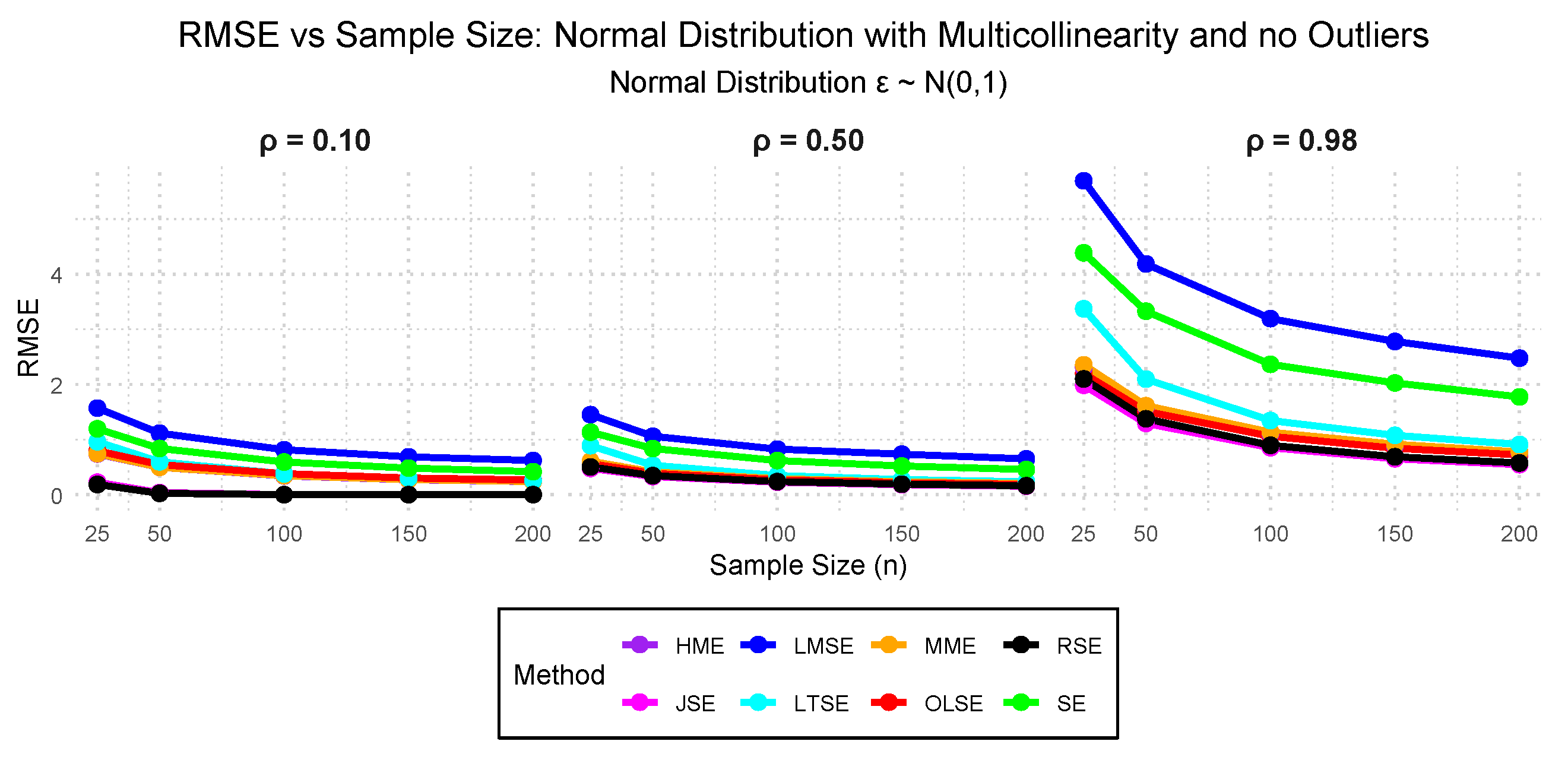
Figure 2.
RMSE Plots under Student’s t-distribution with 7 Degrees of Freedom with Multicollinearity and no Outliers.
Figure 2.
RMSE Plots under Student’s t-distribution with 7 Degrees of Freedom with Multicollinearity and no Outliers.
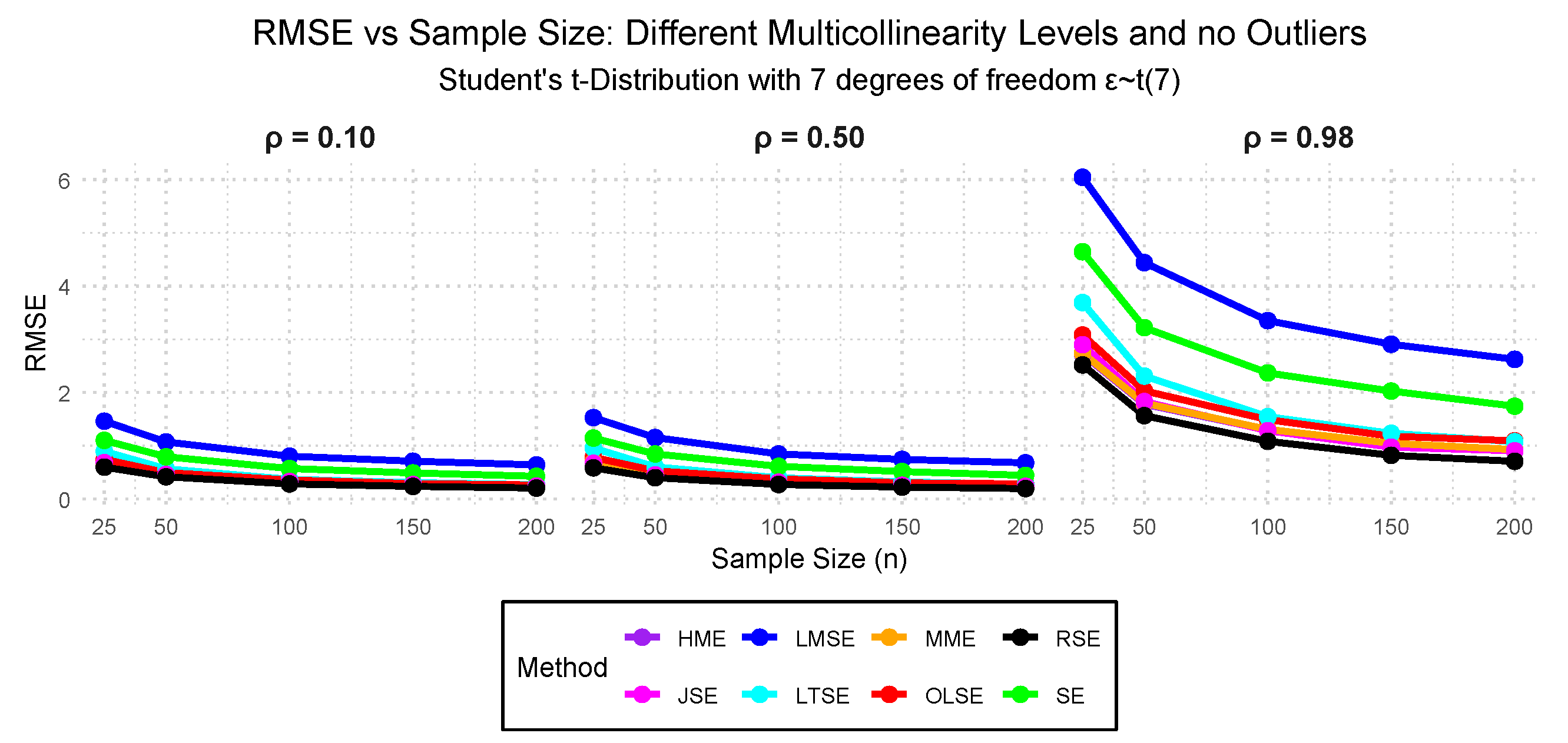
Figure 3.
RMSE Plots under Student’s t-distribution with 2 Degrees of Freedom with Multicollinearity and no Outliers.
Figure 3.
RMSE Plots under Student’s t-distribution with 2 Degrees of Freedom with Multicollinearity and no Outliers.
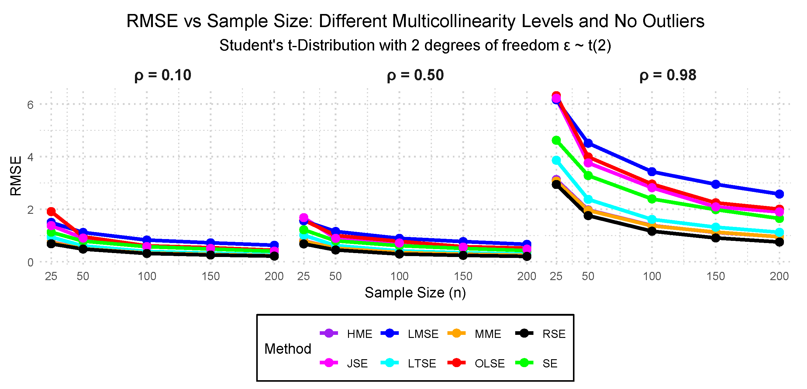
Figure 4.
RMSE Plots under Cauchy Distribution with Multicollinearity and no Outliers.
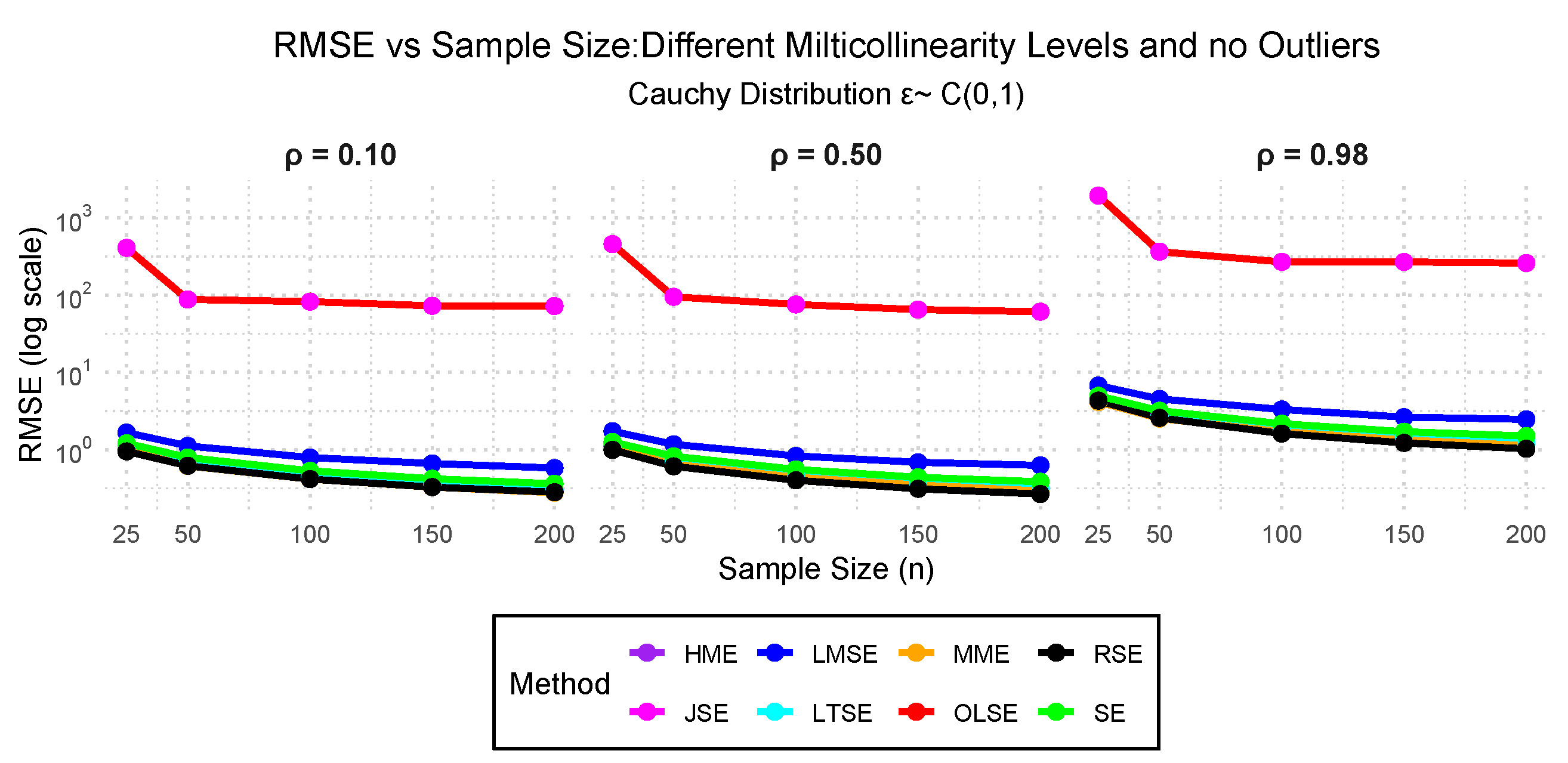
Figure 5.
RMSE Plots under Normal Errors with no Multicollinearity and Outliers in y Direction.
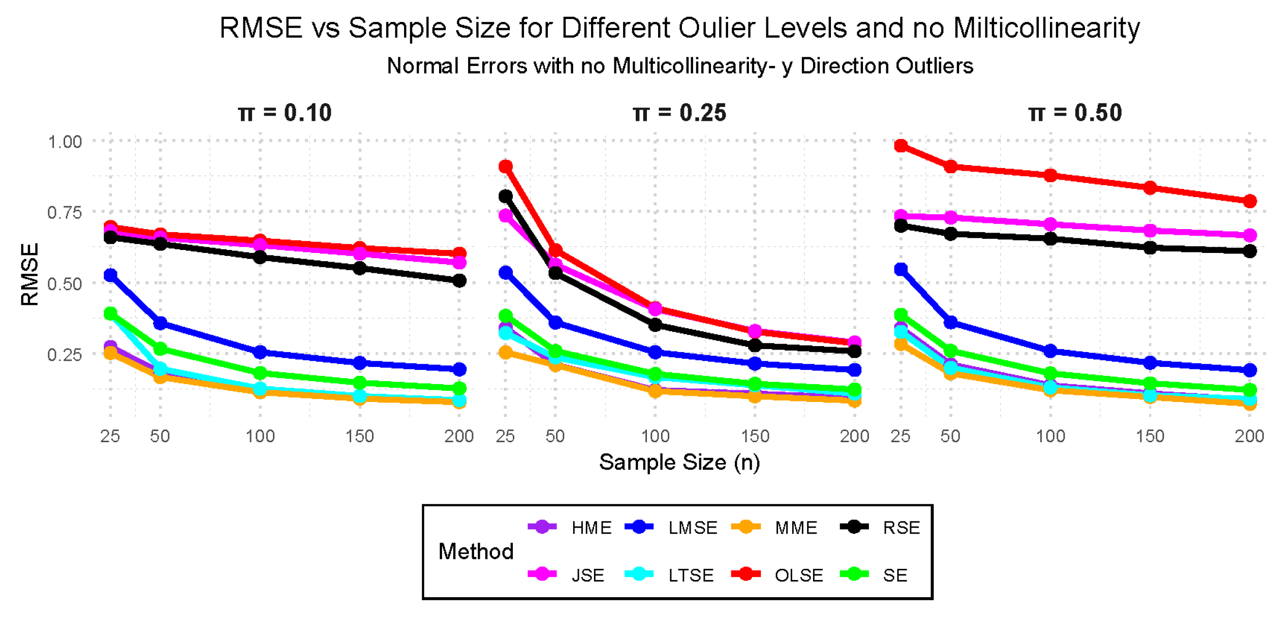
Figure 6.
RMSE Plots with under Normal Errors no Multicollinearity and Outliers in x Direction.
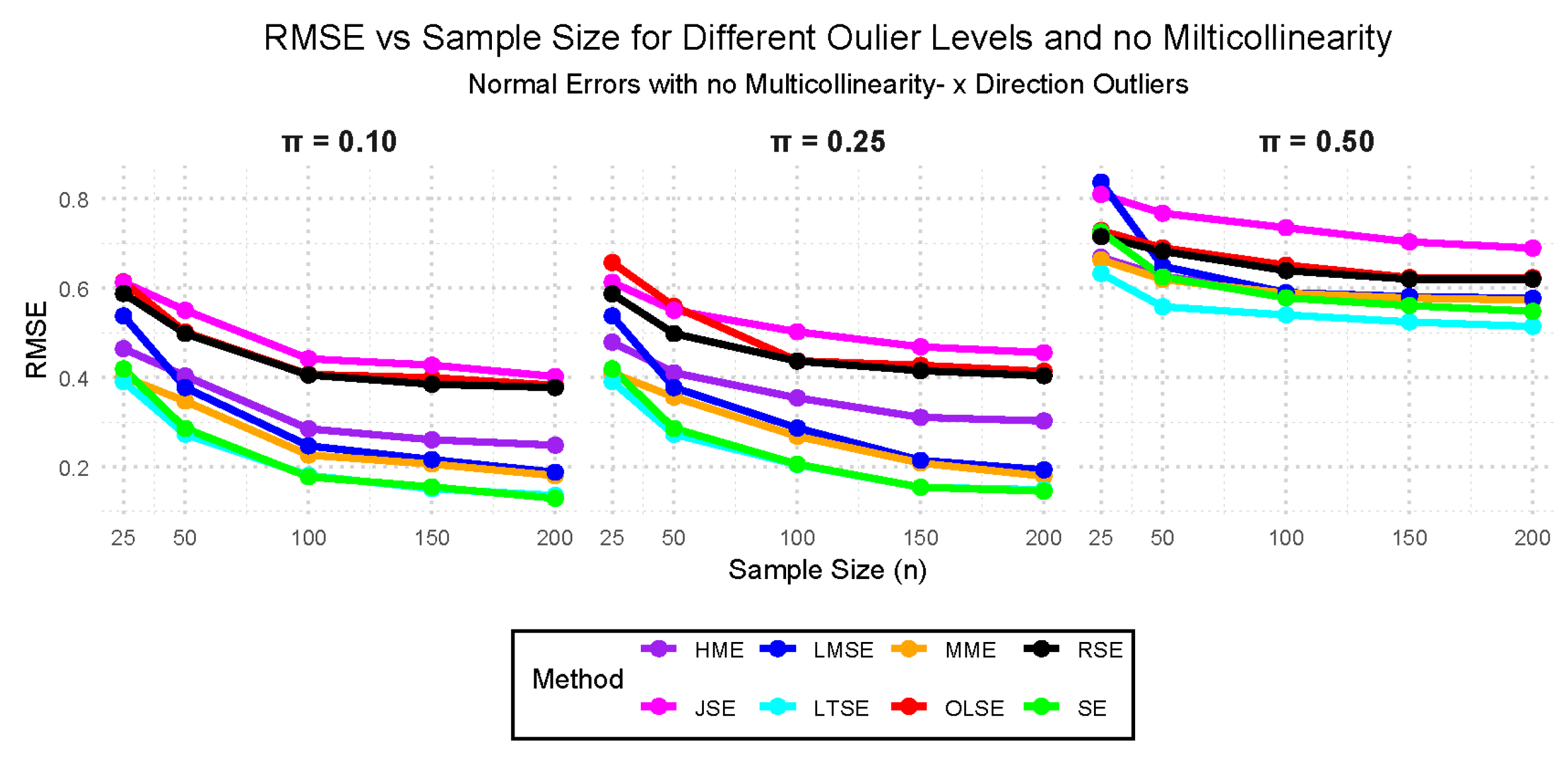
Figure 7.
RMSE Plots with , no Multicollinearity, and Outliers in the y Direction.
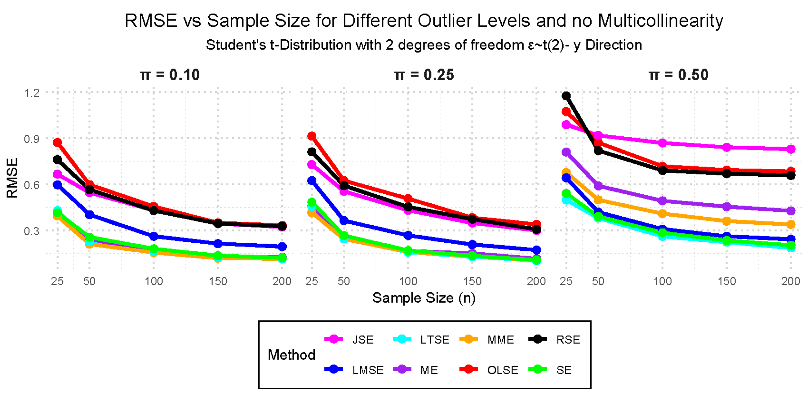
Figure 8.
RMSE Plots with , no Multicollinearity, and Outliers in the x Direction.
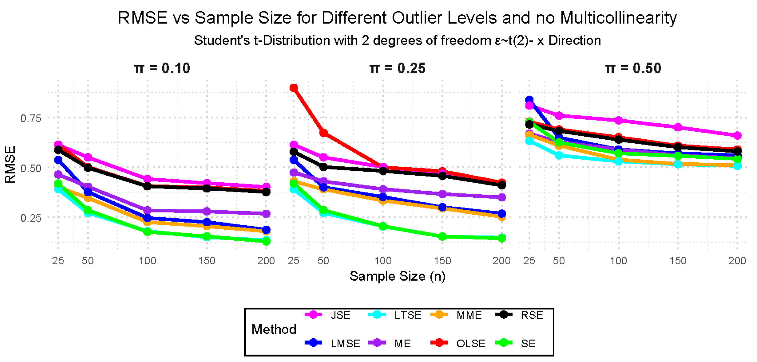
Figure 9.
RMSE Plots with Normal Errors with Multicollinearity, and 10% Outliers in y Direction.
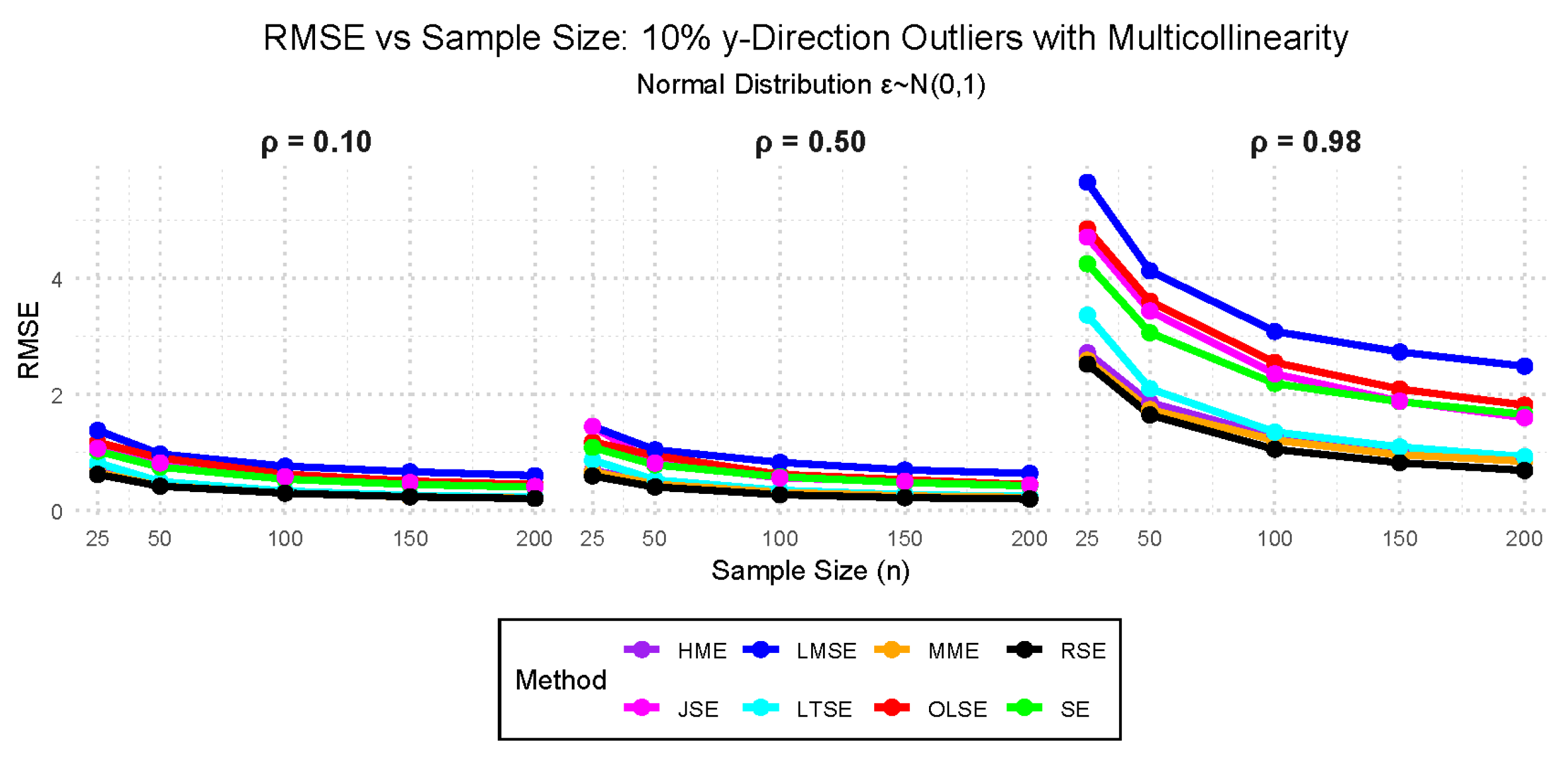
Figure 10.
RMSE Plots with Normal Errors with Multicollinearity, and 25% Outliers in y Direction.

Figure 11.
RMSE Plots with Normal Errors with Multicollinearity, and 50% Outliers in y Direction.
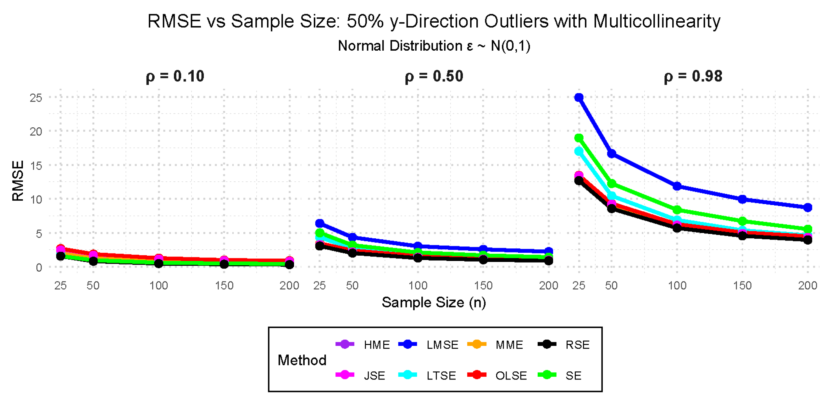
Figure 12.
RMSE Plots for 10% Outliers in x Direction and Multicollinearity
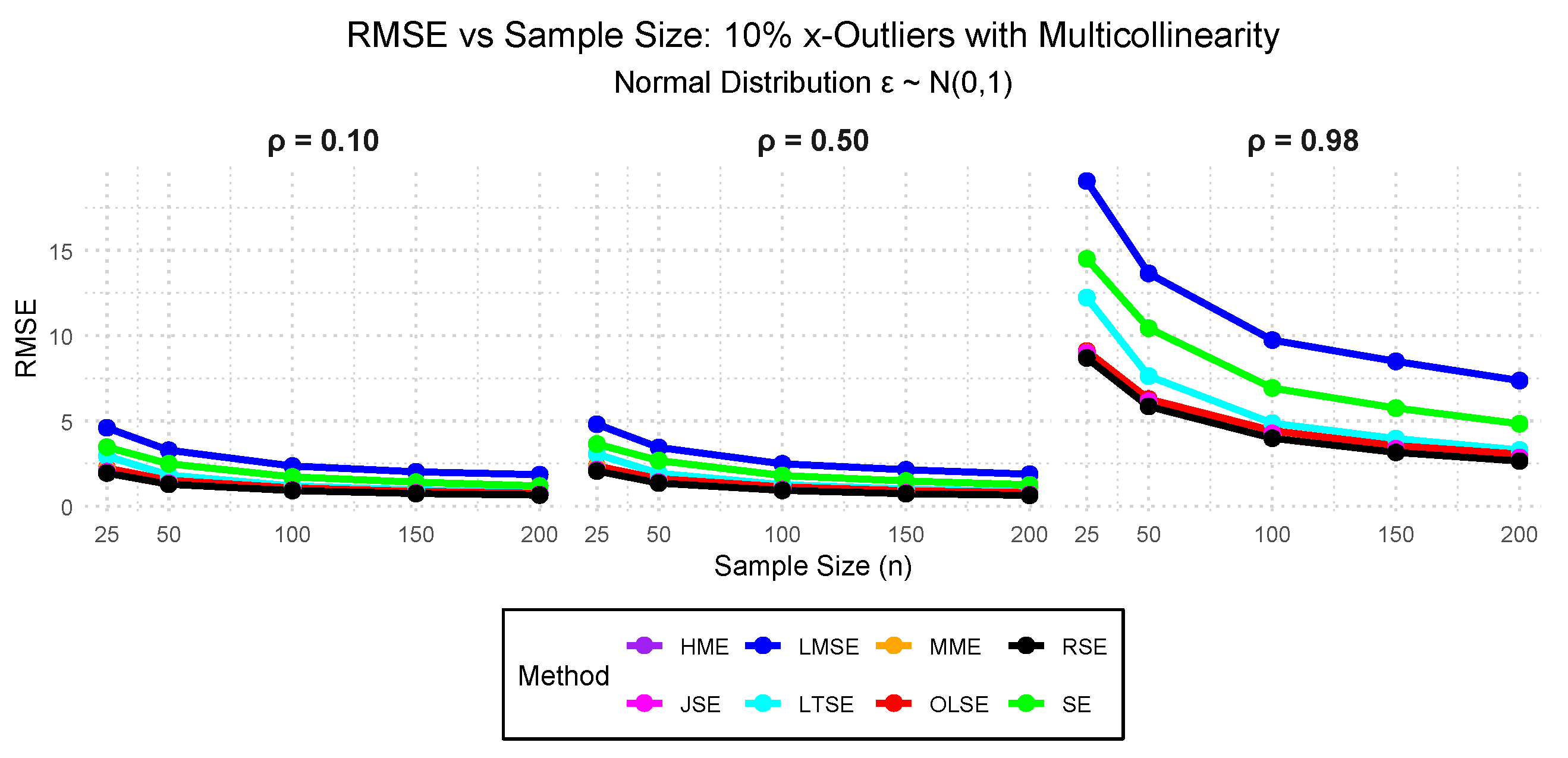
Figure 13.
RMSE Plots with Normal Errors with Multicollinearity, and 25% Outliers in x Direction.
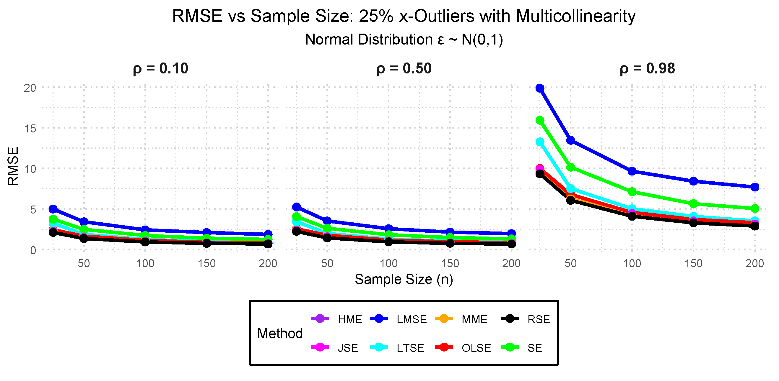
Figure 14.
RMSE Plots with Normal Errors with Multicollinearity, and 50% Outliers in x Direction.
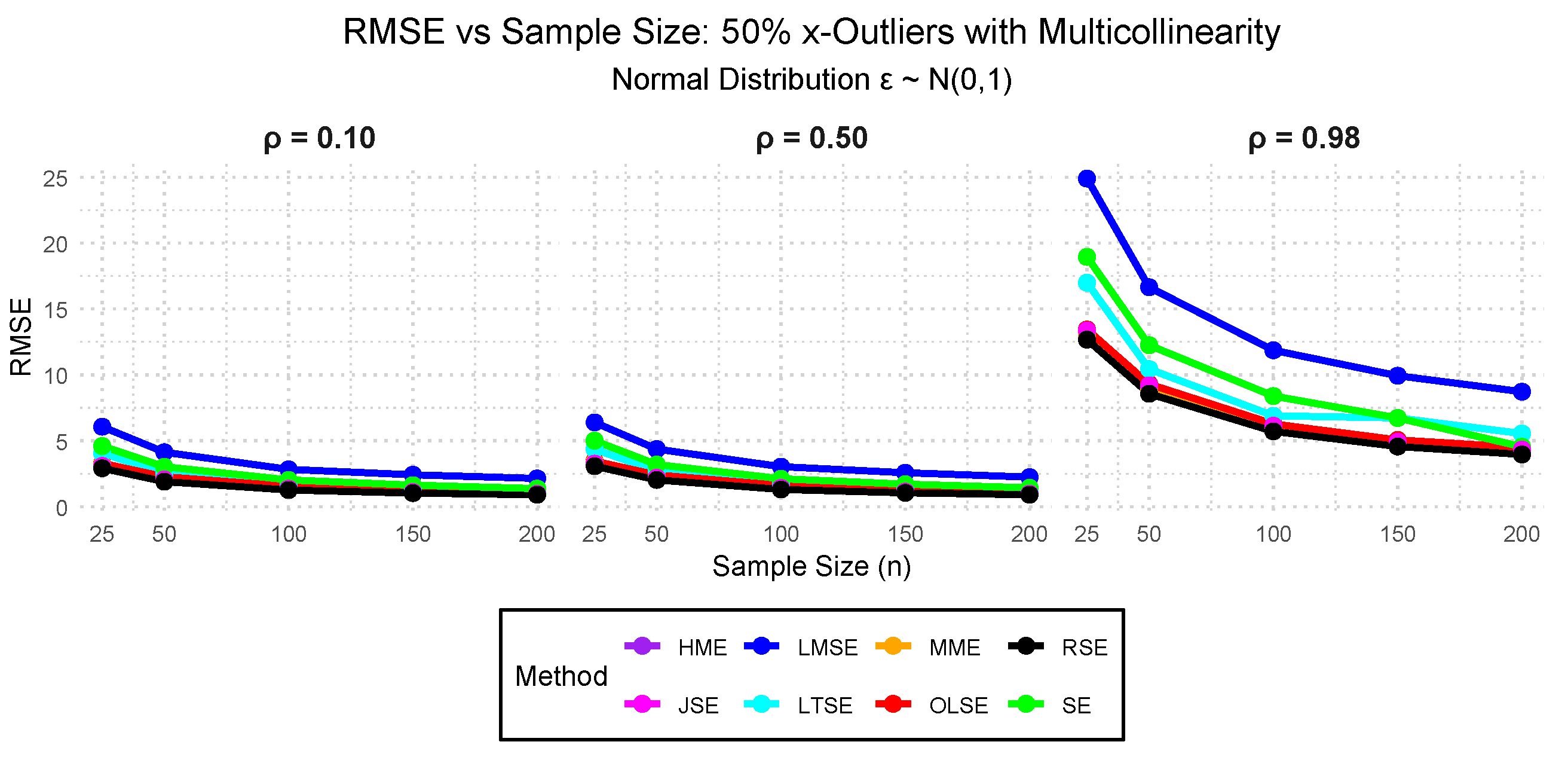
Figure 15.
RMSE Plots with for Different Multicollinearity Levels and 10% y- Outliers.
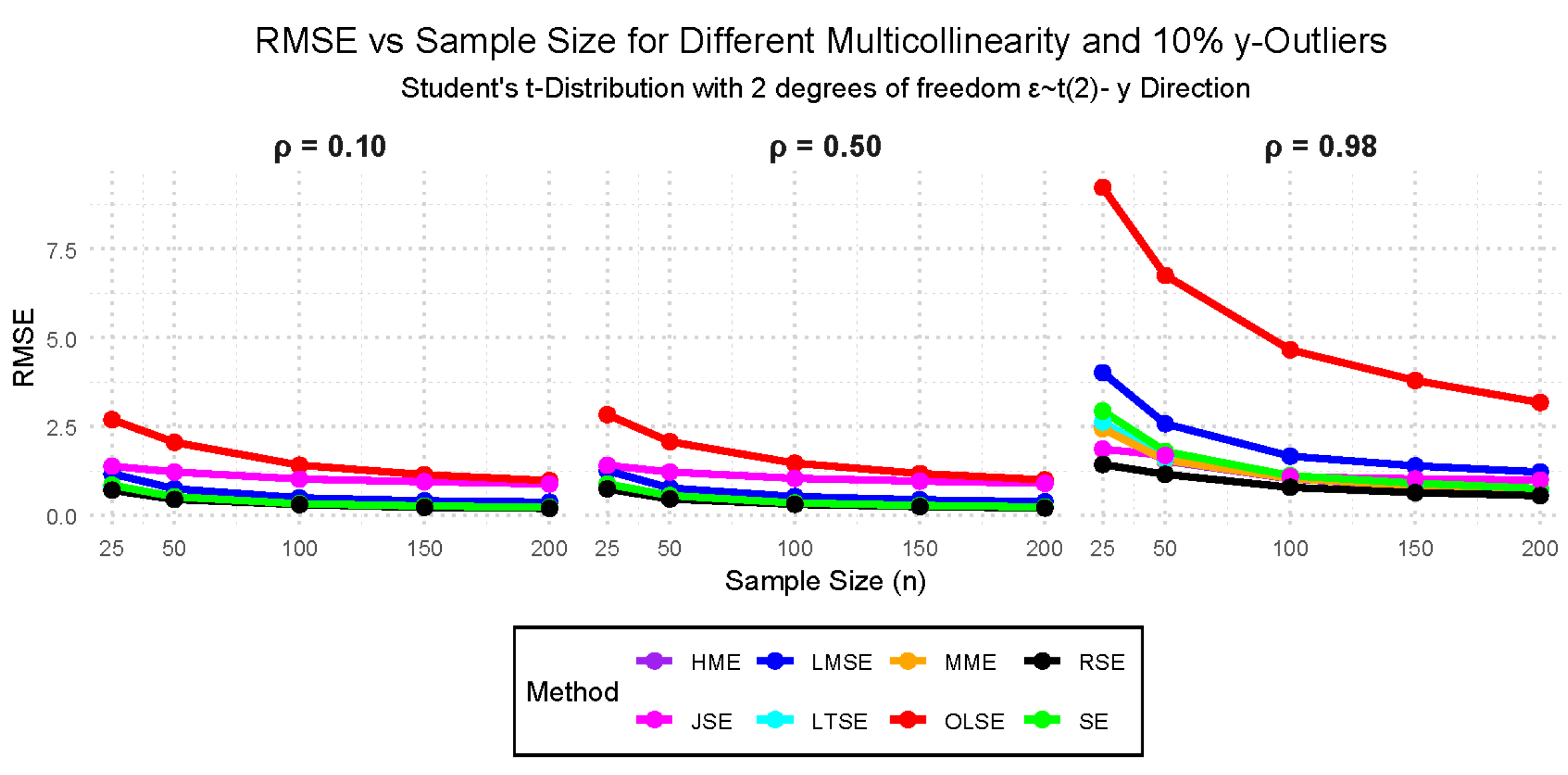
Figure 16.
RMSE Plots with for Different Multicollinearity Levels and 25% y- Outliers.
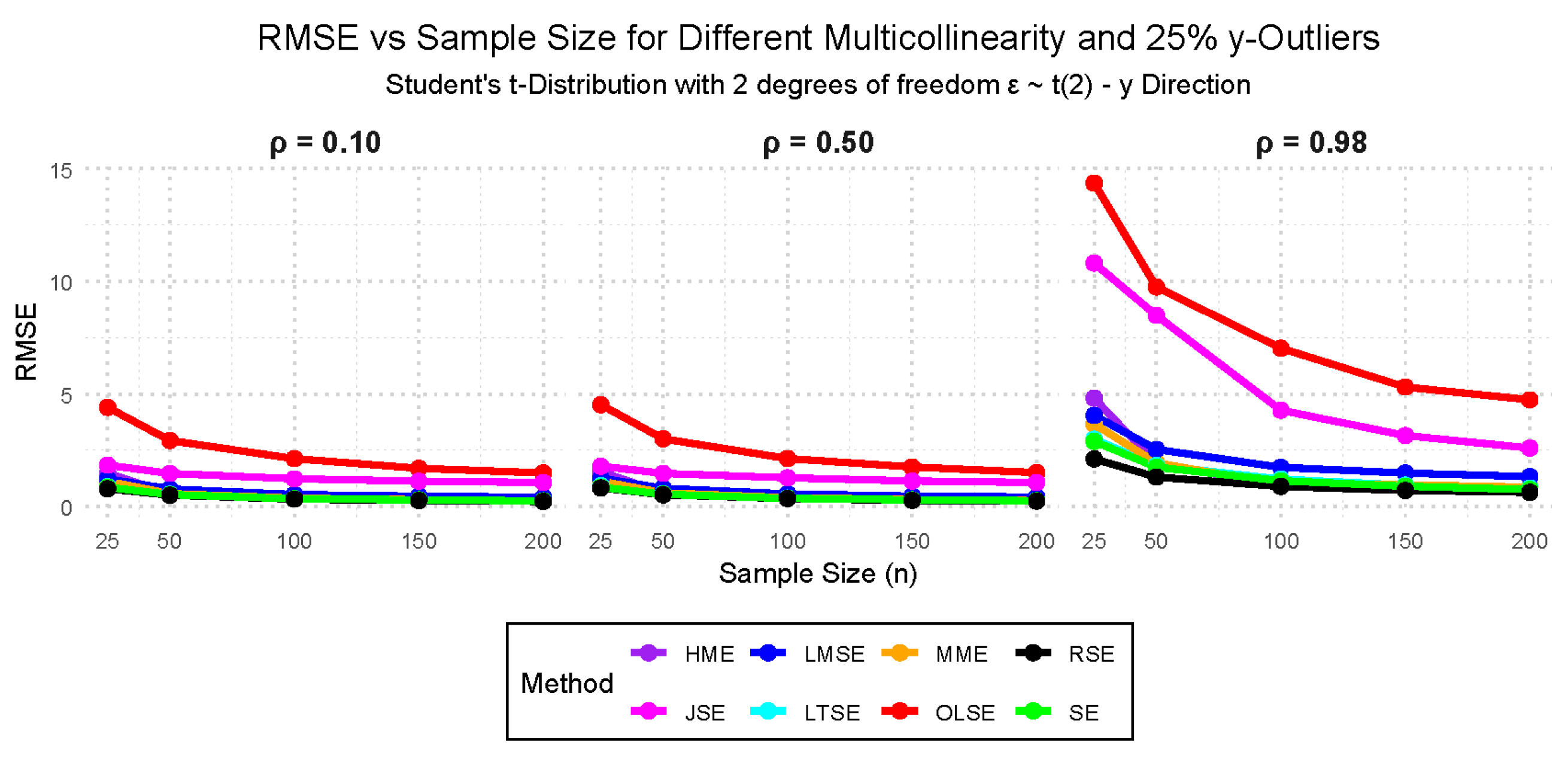
Figure 17.
RMSE Plots with for Different Multicollinearity Levels and 50% y- Outliers.
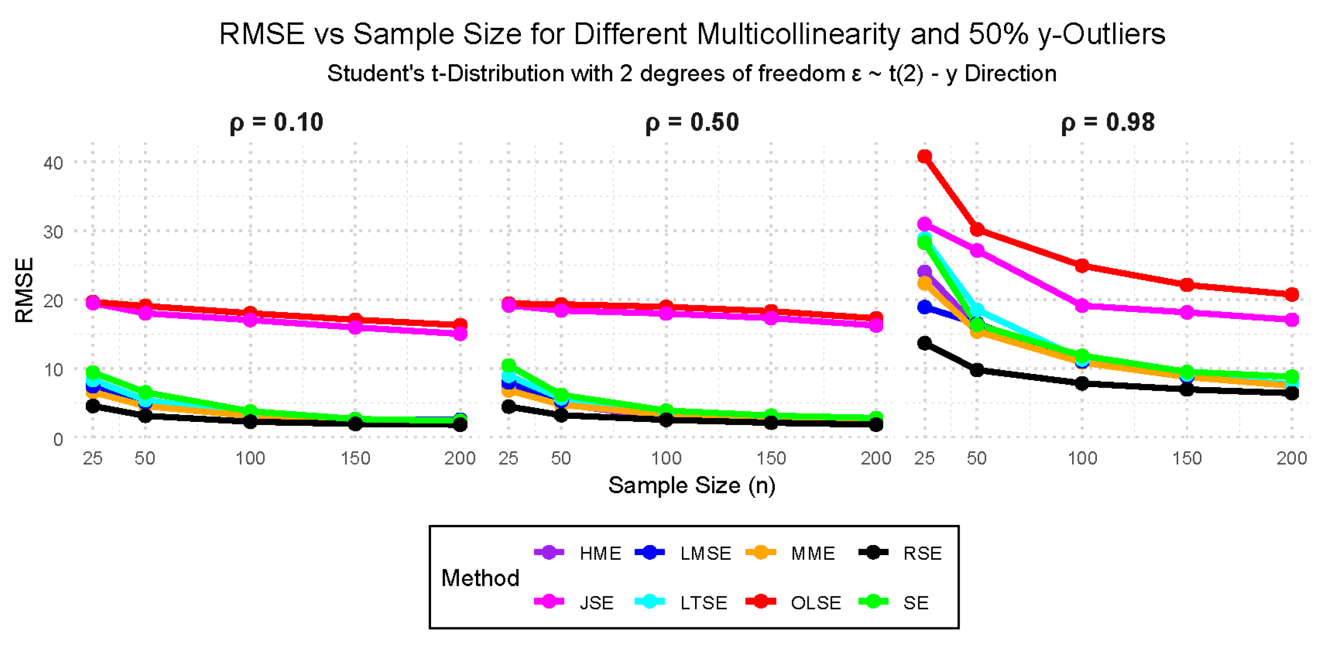
Figure 18.
RMSE Plots with for Different Multicollinearity Levels and 10% x-Outliers.
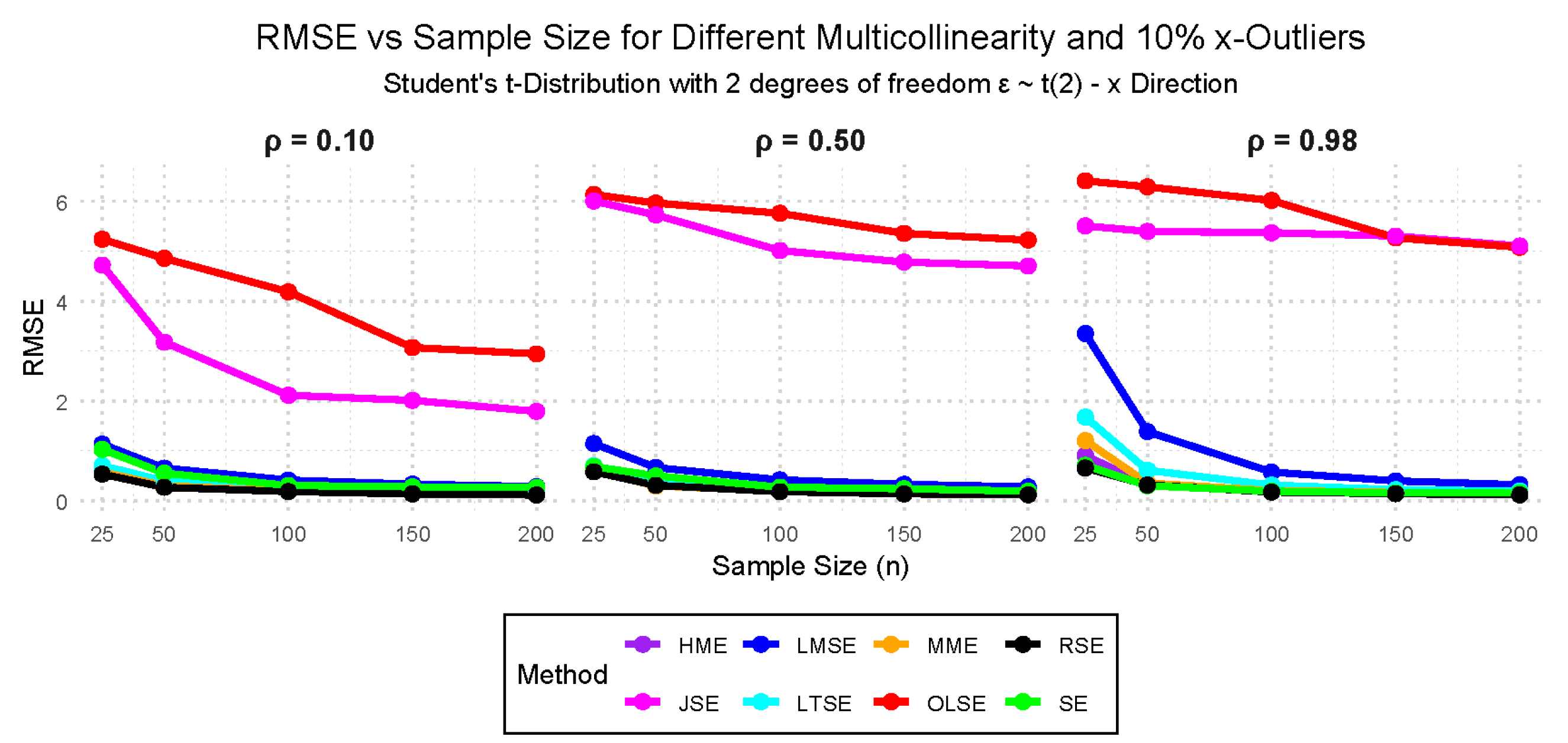
Figure 19.
RMSE Plots with for Different Multicollinearity Levels and 25% x-Outliers.
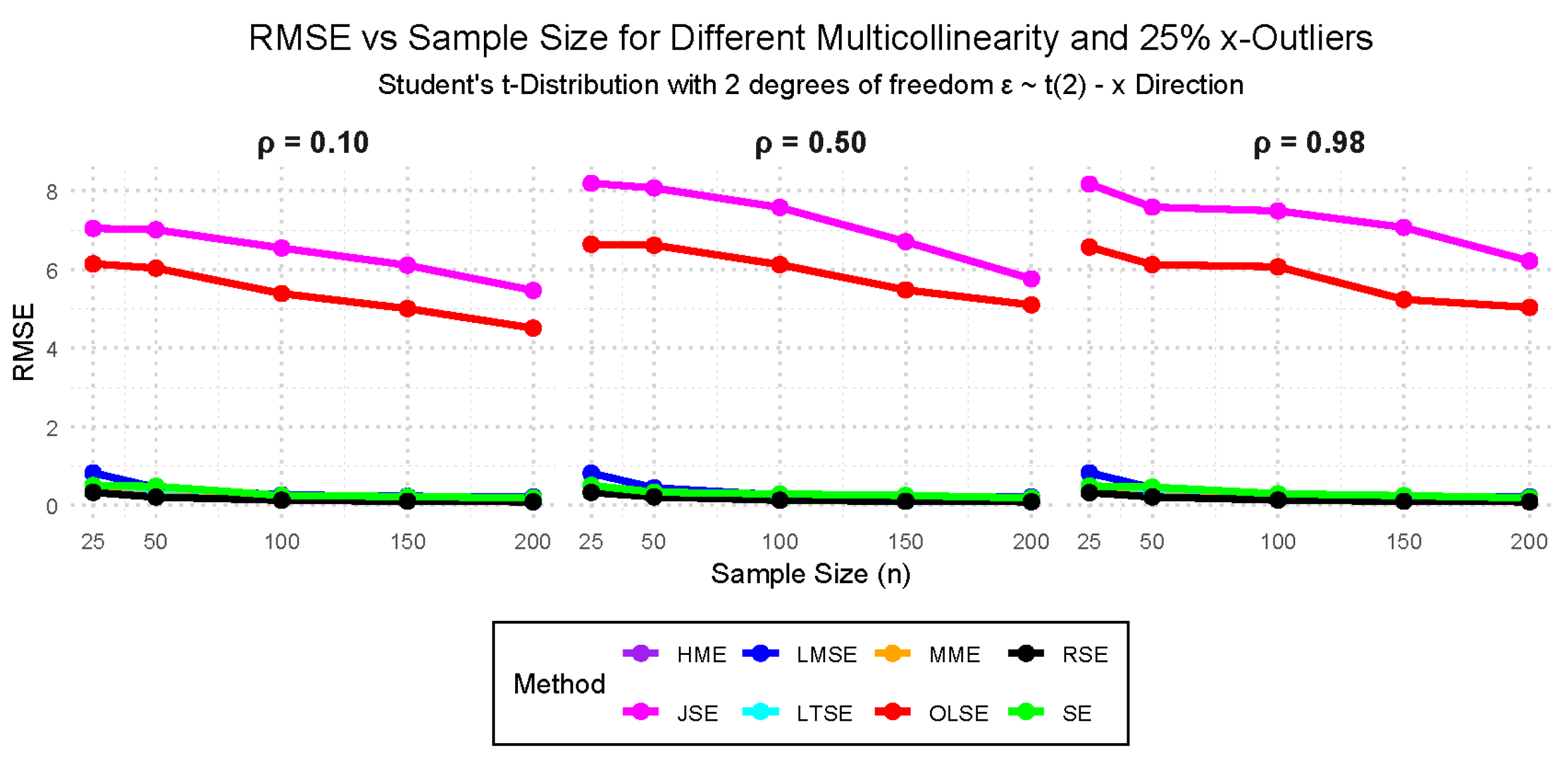
Figure 20.
RMSE Plots with for Different Multicollinearity Levels and 50% x-Outliers.
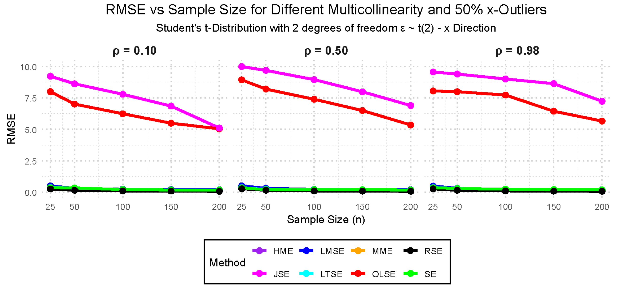
Figure 21.
Plot to Check for Outliers Using a Milk Dataset.
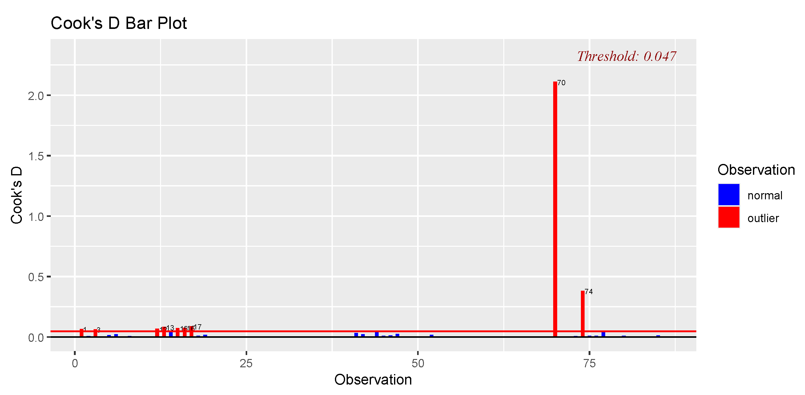
Figure 22.
Plots to Check for Normality on OLS using a Milk Dataset.
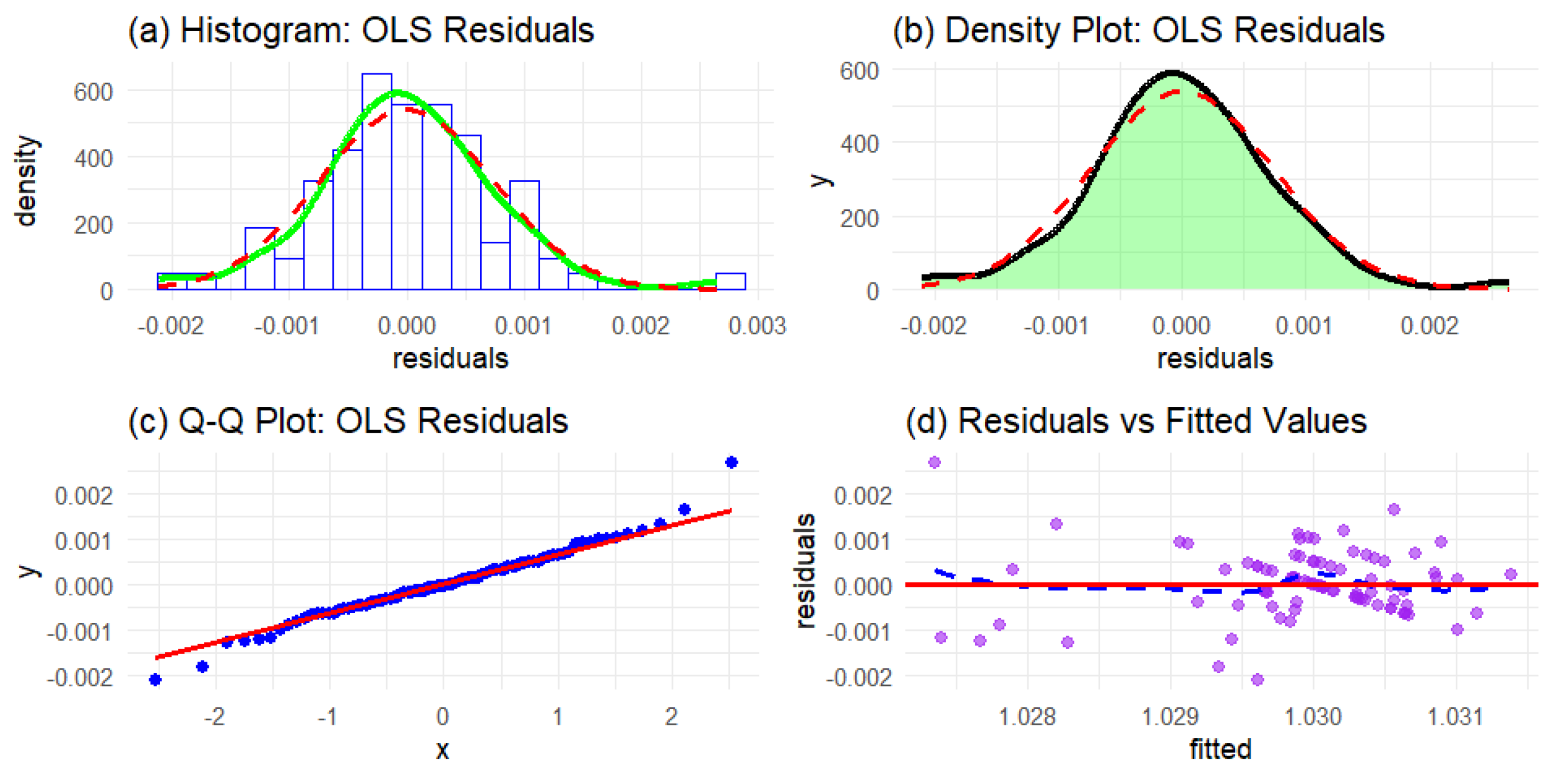
Figure 23.
Comparison of Bias and RMSE Across Multicollinearity and Outlier Levels for Milk Dataset.
Figure 23.
Comparison of Bias and RMSE Across Multicollinearity and Outlier Levels for Milk Dataset.
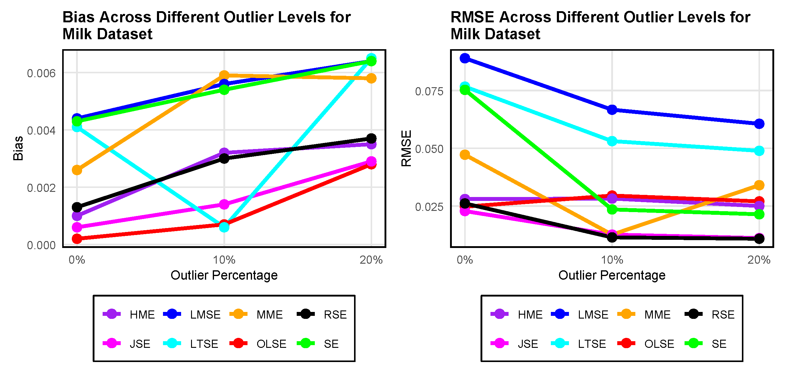
Figure 24.
Plot to Check for Outliers Using a Real Estate Valuation Dataset.
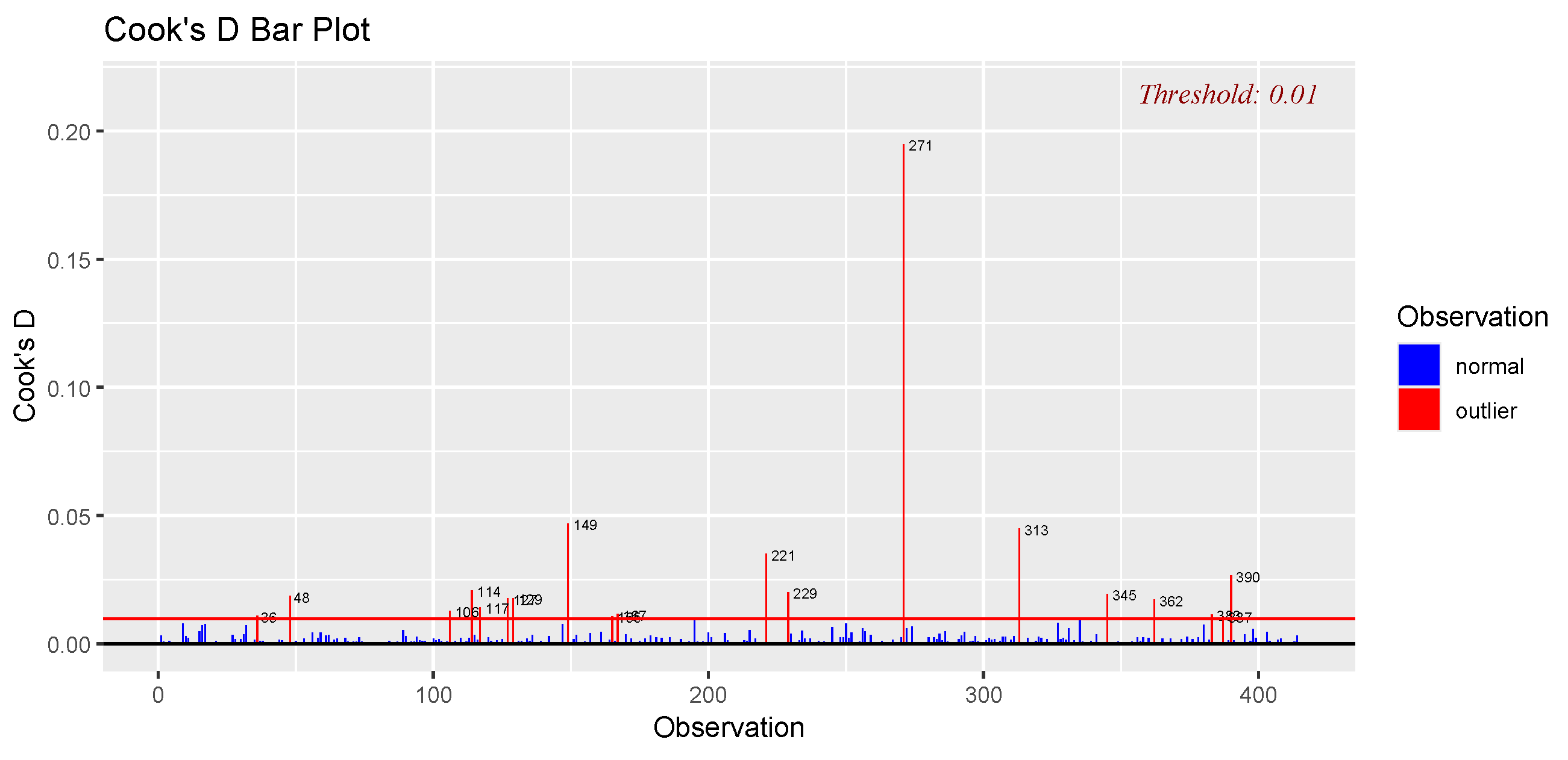
Figure 25.
Plots to Check for Normality on OLS using Real Estate Valuation Dataset.
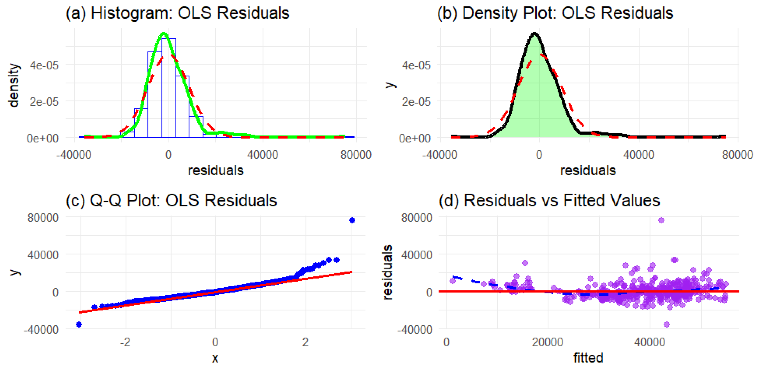
Figure 26.
Comparison of Bias and RMSE Across Multicollinearity and Outlier Levels for Real Estate Valuation Dataset.
Figure 26.
Comparison of Bias and RMSE Across Multicollinearity and Outlier Levels for Real Estate Valuation Dataset.
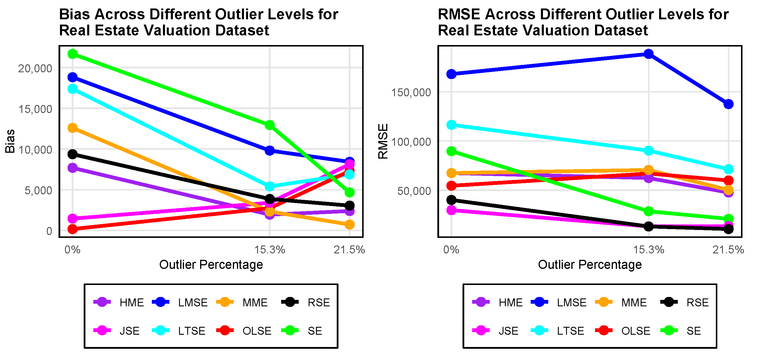
Figure 27.
Plot to Check for Outliers Using a Hawkins Bradu Kass Dataset
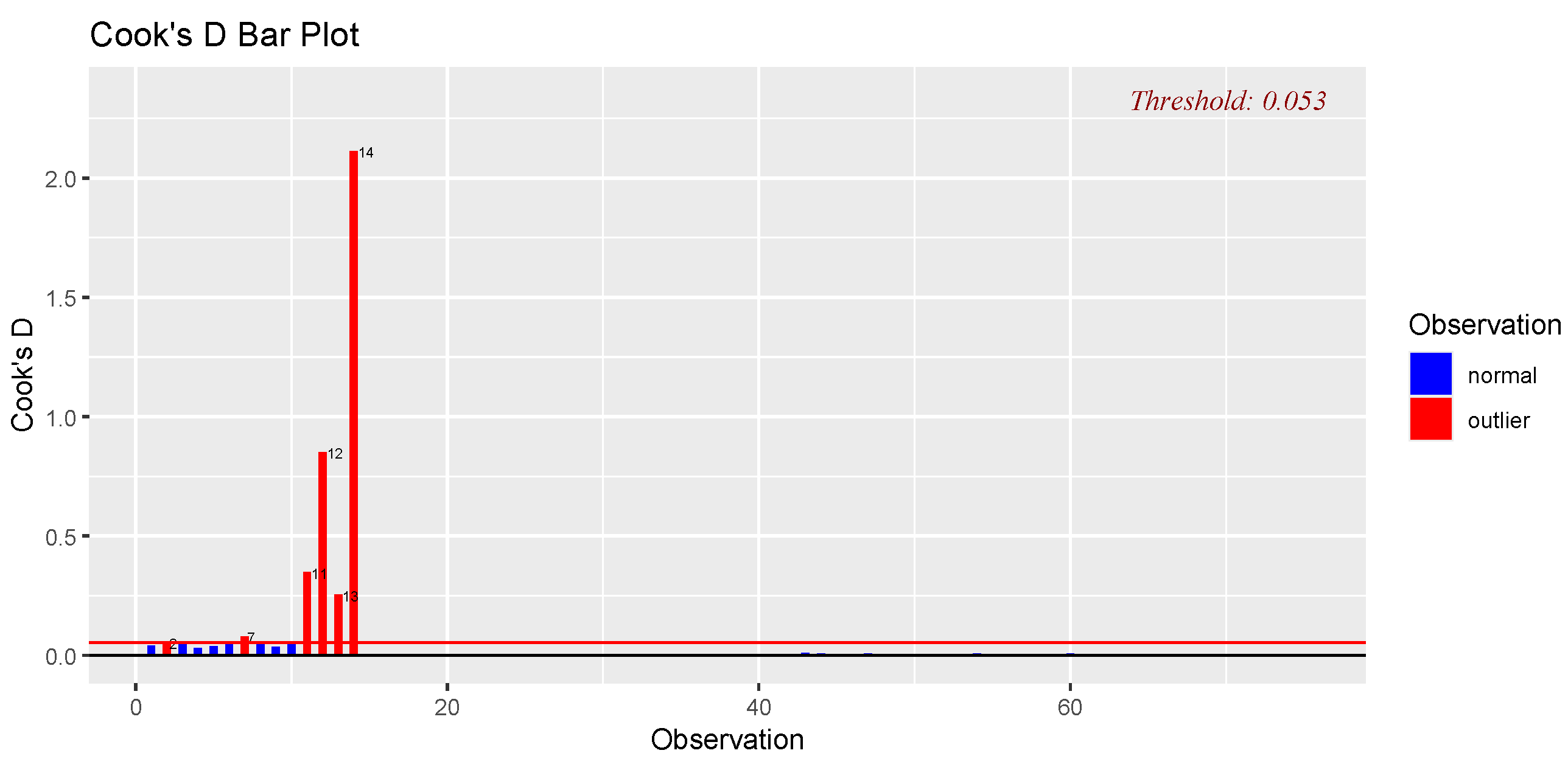
Figure 28.
Plots to Check for Normality on OLS using Hawkins Bradu Kass Dataset

Figure 29.
Comparison of Bias and RMSE Across Multicollinearity and Outlier Levels for Hawkins Bradu Kass Dataset.
Figure 29.
Comparison of Bias and RMSE Across Multicollinearity and Outlier Levels for Hawkins Bradu Kass Dataset.
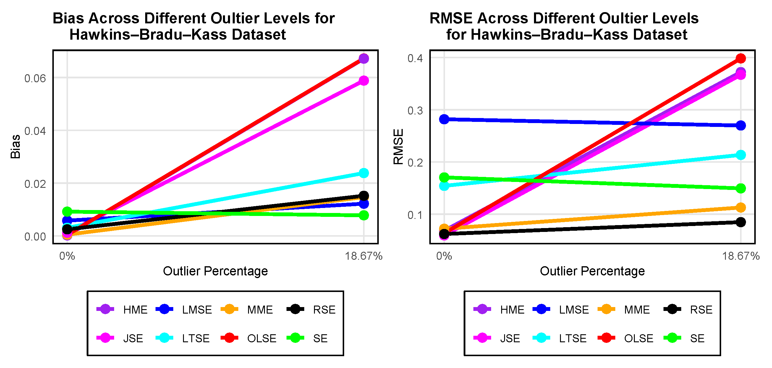
Table 2.
Pearson Correlation Coefficient Matrix of the Regressors for the Milk Dataset.
| 1.0000 | 0.4496 | 0.4055 | 0.3235 | 0.3588 | 0.6748 | 0.6480 | |
| 0.4496 | 1.0000 | 0.9248 | 0.6288 | 0.6382 | 0.7010 | 0.6380 | |
| 0.4055 | 0.9248 | 1.0000 | 0.5866 | 0.5959 | 0.6963 | 0.6380 | |
| 0.3235 | 0.6288 | 0.5866 | 1.0000 | 0.9782 | 0.5469 | 0.3897 | |
| 0.3588 | 0.6382 | 0.5959 | 0.9782 | 1.0000 | 0.5666 | 0.4292 | |
| 0.6748 | 0.7010 | 0.6963 | 0.5469 | 0.5666 | 1.0000 | 0.6827 | |
| 0.6480 | 0.6380 | 0.6380 | 0.3897 | 0.4292 | 0.6827 | 1.0000 |
Table 3.
Estimated Bias and RMSE of the Estimators under Multicollinearity and Varying Outlier Levels for Milk Dataset.
Table 3.
Estimated Bias and RMSE of the Estimators under Multicollinearity and Varying Outlier Levels for Milk Dataset.
| Estimator | 0% Outlier | 10% Outlier | 20% Outlier | |||
|---|---|---|---|---|---|---|
| Bias | RMSE | Bias | RMSE | Bias | RMSE | |
| OLSE | 0.0002 | 0.0247 | 0.0007 | 0.0295 | 0.0028 | 0.0270 |
| HME | 0.0010 | 0.0280 | 0.0032 | 0.0282 | 0.0035 | 0.0250 |
| MME | 0.0026 | 0.0472 | 0.0059 | 0.0126 | 0.0058 | 0.0340 |
| LMSE | 0.0044 | 0.0890 | 0.0056 | 0.0667 | 0.0064 | 0.0606 |
| LTSE | 0.0041 | 0.0767 | 0.0006 | 0.0531 | 0.0065 | 0.0489 |
| SE | 0.0043 | 0.0753 | 0.0054 | 0.0235 | 0.0064 | 0.0214 |
| JSE | 0.0006 | 0.0228 | 0.0014 | 0.0126 | 0.0029 | 0.0111 |
| RSE | 0.0013 | 0.0261 | 0.0030 | 0.0114 | 0.0037 | 0.0108 |
Table 4.
Pearson Correlation Coefficient Matrix of the Regressors for the Real Estate Valuation Dataset.
Table 4.
Pearson Correlation Coefficient Matrix of the Regressors for the Real Estate Valuation Dataset.
| 1.0000 | 0.0175 | 0.0609 | 0.0095 | 0.0350 | ||
| 0.0175 | 1.0000 | 0.0256 | 0.0496 | 0.0544 | ||
| 0.0609 | 0.0256 | 1.0000 | -0.6025 | -0.5911 | -0.8063 | |
| 0.0095 | 0.0496 | -0.6025 | 1.0000 | 0.4441 | 0.4491 | |
| 0.0350 | 0.0544 | -0.5911 | 0.4441 | 1.0000 | 0.4129 | |
| -0.8063 | 0.4491 | 0.4129 | 1.0000 |
Table 5.
Estimated Bias and RMSE of the Estimators under Multicollinearity and Varying Outlier Levels for Real Estate Valuation Dataset.
Table 5.
Estimated Bias and RMSE of the Estimators under Multicollinearity and Varying Outlier Levels for Real Estate Valuation Dataset.
| Estimator | 0% Outlier | 15.3% Outlier | 21.5% Outlier | |||
|---|---|---|---|---|---|---|
| Bias | RMSE | Bias | RMSE | Bias | RMSE | |
| OLSE | 168.2679 | 54504.9900 | 2732.8280 | 66897.1350 | 7291.0330 | 59865.6200 |
| HME | 7683.2360 | 67391.2100 | 1937.2760 | 62329.2885 | 2379.8690 | 47601.0400 |
| MME | 12588.7800 | 67391.2100 | 2322.3150 | 70523.8053 | 720.0933 | 50175.4500 |
| LMSE | 18806.2100 | 167922.3000 | 9802.2880 | 188380.7012 | 8417.1460 | 137477.5000 |
| LTSE | 17386.5200 | 116365.6000 | 5397.6670 | 90165.8498 | 6875.5230 | 71319.8900 |
| SE | 21667.5800 | 89613.2900 | 12931.5900 | 28573.5115 | 4669.2530 | 20823.2300 |
| JSE | 1446.8980 | 29700.3800 | 3393.4700 | 13195.9917 | 8122.0880 | 13441.6400 |
| RSE | 9355.8480 | 40048.4200 | 3861.2500 | 13122.0683 | 3046.3670 | 10501.8300 |
Table 6.
Pearson Correlation Coefficient Matrix of the Regressors for Hawkins Bradu Kass Dataset.
| 1.0000 | 0.9460 | 0.9618 | |
| 0.9460 | 1.0000 | 0.9787 | |
| 0.9618 | 0.9787 | 1.0000 |
Table 7.
Estimated Bias and RMSE of the Estimators under Multicollinearity and Varying Outlier Levels for Hawkins–Bradu–Kass Dataset.
Table 7.
Estimated Bias and RMSE of the Estimators under Multicollinearity and Varying Outlier Levels for Hawkins–Bradu–Kass Dataset.
| Estimator | 0% Outlier | 18.67% Outlier | ||
|---|---|---|---|---|
| Bias | RMSE | Bias | RMSE | |
| OLSE | 0.0004 | 0.0633 | 0.0672 | 0.3983 |
| HME | 0.0002 | 0.0683 | 0.0671 | 0.3721 |
| MME | 0.0005 | 0.0721 | 0.0147 | 0.1127 |
| LMSE | 0.0058 | 0.2818 | 0.0122 | 0.2698 |
| LTSE | 0.0031 | 0.1542 | 0.0238 | 0.2135 |
| SE | 0.0092 | 0.1704 | 0.0078 | 0.1494 |
| JSE | 0.0012 | 0.0593 | 0.0588 | 0.3669 |
| RSE | 0.0025 | 0.0620 | 0.0152 | 0.0847 |
Disclaimer/Publisher’s Note: The statements, opinions and data contained in all publications are solely those of the individual author(s) and contributor(s) and not of MDPI and/or the editor(s). MDPI and/or the editor(s) disclaim responsibility for any injury to people or property resulting from any ideas, methods, instructions or products referred to in the content. |
© 2025 by the authors. Licensee MDPI, Basel, Switzerland. This article is an open access article distributed under the terms and conditions of the Creative Commons Attribution (CC BY) license (http://creativecommons.org/licenses/by/4.0/).
Copyright: This open access article is published under a Creative Commons CC BY 4.0 license, which permit the free download, distribution, and reuse, provided that the author and preprint are cited in any reuse.


