
Submitted:
07 April 2025
Posted:
08 April 2025
You are already at the latest version
Abstract
This paper introduces ridge‐type kernel smoothing estimators for par-tially linear time‐series models that employ shrinkage estimation to han-dle autoregressive errors and severe multicollinearity in the parametric component. By combining a generalized ridge penalty with kernel smoothing, the proposed estimators solve inflated variances arising from linear dependencies among predictors, while also accounting for auto-correlation. Four well-known selection criteria—Generalized Cross Val-idation (GCV), Improved Akaike Information Criterion (AICc), Bayesian Information Criterion (BIC), and Risk Estimation via Classical Pilots (RECP)—are used to optimally choose both the bandwidth and shrinkage parameters. We provide closed‐form expressions for these estimators, establish their asymptotic properties, and present a risk‐based analysis that highlights the benefits of ordinary and positive‐part shrinkage ex-tensions. Simulation studies confirm that the introduced shrinkage ap-proaches outperforms standard methods when predictors are strongly correlated, with this advantage growing as sample sizes increase. An ap-plication to airline delay time‐series data further illustrates the efficacy and practical interpretability of the introduced methodology.
Keywords:
Shrinkage estimation
; partially linear models
; multicollinearity
; ridge-type kernel smoother
; parameter selection
MSC: 62G08; 62J07; 62M10
1. Introduction
In many time-series applications, one must balance interpretability and flexibility in modeling. Partially linear regression models achieve this by expressing the response as a parametric linear function of some covariates alongside a nonparametric smooth function of an additional variable. Specifically, we consider the following model setup:
(1.1)
where denotes stationary response at time , and its prediction depends on the p-dimensional vector of explanatory variables with and an extra univariate variable . Also, is an unknown p-dimensional parameter vector to be estimated, is an unknown smooth function, and are the error terms.
Unlike classical linear models, (1.1) offers the interpretability of while retaining the capacity to model complex, nonlinear effects through ([14]; Robinson, 1998). However, two mojor issues often arise:
Multicollinearity among When the columns of are nearly linearly dependent, ordinary least squares (OLS) or unpenalized nonparametric estimators can have extremely high variances [10].
Autocorrelation or dependence among , as is common in time-series or longitudinal settings. We capture this by a first-order autoregressive process:
(1.2)
ensuring that is stationarily dependent over time ([7,15]). Also, to simplify the notational illustration, a matrix–vector form of the model (1.1) can be stated as
(1.3)
where, , and. The main goal is to estimate the unknown parameter vector , the smooth function and the mean vector based on the observations from the data set {}. Partially linear models enable easier interpretation of the effect of each variable and owing to the “curse of dimensionality”, these models can be preferred to a completely nonparametric regression model. Specifically, partially linear models are more practical than the classical linear model because they combine both parametric part presented numerically and nonparametric part displayed graphically.
Eventhough partially linear models have specific advantages, these models typically assume uncorrelated errors ([6,8,14]). In real-world time-series or panel data, ignoring (1.2) can degrade efficiency and produce biased inferences ([11,19]). Moreover, multicollinearity among amplifies these problems, inflating variances to the point that estimates become unreliable ([13,20]).
To mitigate these issues, we adopt ridge-type kernel smoothing for the parametric component. In essence, a shrinkage penalty is added so that the linear portion is “shrunk” toward zero to stabilize estimation. Mathematically, for instance, a ridge-type kernel (RTK) estimator of can be expressed (after suitable data transformation) as in (2.3) which has been extensively studied by [17]. This ridge-inspired framework stems from Stein-type shrinkage theory, which shows that biased estimators can dominate unbiased ones, particularly in moderate-to-high dimensions or under strong correlation ([1,2]). Indeed, Stein’s paradox reveals that for shrinking an estimator can lower the overall mean squared error despite introducing bias, a phenomenon extensively explored by [1,3]).
When errors follow (1.2), we further incorporate transformations to handle the autocovariance structure, yielding generalized ridge-type kernel (GRTK) estimators that optimally exploit the correlation . These GRTK methods align with earlier biased estimation approaches for linear or partially linear models with correlated errors ([13,20,21]). By merging the Stein-type shrinkage logic with kernel smoothing, one obtains robust estimators of both and that effectively address multicollinearity and autocorrelation in a unified fashion.
In this paper, we formalize and extend such modified ridge-type kernel smoothing estimators for partially linear time-series models. We focus on:
The precise data transformation to accommodate (1.2).
The interplay between shrinkage and the bandwidth for kernel smoothing.
Selecting these tuning parameters () using multiple criteria, including GCV, AICc, BIC, and RECP.
This framework is motivated by [3] broader research on shrinkage-based variable selection and penalty methods, which shows that penalized procedures (including ridge, lasso, and Stein-like estimators) can vastly reduce variance in semiparametric regressions—particularly with correlated data or limited samples. Consequently, the main goal is to fill a gap in semiparametric regression by uniting autoregressive error modeling (1.2), handling with multicollinearity and Stein-type shrinkage in kernel-based estimation.
The rest of the paper is organized as follows. Section 2 explains how we fit the autoregressive structure (1.2) and handle collinearity. Section 3 provides the mathematical formulations of our GRTK shrinkage estimators for both and the smooth function , including asymptotic properties. Section 4 details the procedures for choosing and bandwidth . Section 5 illustrates, through extensive simulation and an airline delay time-series dataset, how the proposed methodology outperforms traditional methods under multicollinearity and autocorrelation. Finally, Section 6 concludes with a discussion of key findings and future research directions.
2. Fitting the Model Error Structure
Assume that ′ is a realization from a stationary time series described by model (1.1) with autoregressive error terms satisfying the following assumption.
Assumption 2.1: The error is a stationary dependent sequence with and for some constant Letting and , where is a positive definite symmetric matrix.
Here, Assumption 2.1 is standard in time-series analysis because it allows for modeling of stationary errors with finite variance. Such an assumption is common in many time-series models where the error term’s statistical properties remain constant over time. Note that the autoregressive errors follow an dimensional multivariate normal distribution with a mean zero and stationary covariance matrix . We may also write this expression in the equivalent form , where is a covariance matrix, given by
(2.1a)
with the inverse
(2.1b)
where denotes the correlation between and , as defined before. It should be emphasized that once we have an estimate of the parameter vector and an estimator of the unknown smooth function , the parameter can be estimated by the residuals from the semiparametric regression , defined as
There are several methods to estimate and In this work, we adopt the ridge type kernel (RTK) method discussed by [17], generalizes partial kernel method proposed by [14]. Specifically, the RTK estimator of is the form
(2.3)
where is a shrinkage parameter, is an identity matrix, , , and is a kernel smoother matrix of weights satisfying the satisfying Assumption (2.3), given by
where is a bandwidth parameter to selected, and is kernel function defined in Remark 2.2. For example, could be Gaussian, Epanechnikov, etc. Then, an estimator of the nonparametric part is obtained by
(2.5)
Hence, the autoregressive coefficient arises from (2.2) and the noise of the AR(1) is obtained by . Note that since the errors in the model (1.1) are serially correlated, the estimators defined in (2.3) and (2.5) is not asymptotically efficient. To improve efficiency, we use kernel ridge type weighted estimation based on transforming data .
3. Generalized Ridge Type Kernel Estimation
The generalized ridge type kernel (GRTK) estimator of the parametric components in the model (1.1) is constructed by combining the partial kernel method with a suitable transformation to account for in the AR(1) errors. We will then extend this GRTK estimator to incorporate shrinkage estimation, analyze its asymptotic properties, and discuss its statistical characteristics. For simplicity, assume the true parameter vector and true error covariance matrix are given. From the , one can see that . Thus, for a given , the natural estimator of the nonparametric component is
where is a kernel smoother matrix, as defined in (2.4). Since defined in Assumption (2.1) is positive definite, there exists a dimensional matrix such that. We first assume that the matrix and, hence, are known. Then, we fit the error structure by the following residuals:
(3.2)
Here, as defined in (2.3), and are locally centered residuals of and , respectively. By considering these partial residuals, the GRTK estimator of the vector is obtained by minimizing the following weighted least squares (WLS) equation.
(3.3)
where denotes the Euclidean norm, is a shrinkage parameter to be selected by a selection method, and are the centered residuals, as defined in (2.3). Also, is a kernel smoothing matrix based on a bandwidth parameter to be selected.
Algebraically, after some operations, the solution of the equation yields the following GRTK estimator:
(3.4)
Replacing in the (3.1) with the in (3.4) to produce an GRTK estimator of the nonparametric component in the partially linear model given by
This section details the construction of the Generalized Ridge-Type Kernel (GRTK) estimator for the parametric component in model (1.1). This is achieved by combining the partial kernel method with a suitable transformation that accounts for in the AR(1) errors. We will then extend this GRTK estimator to incorporate shrinkage estimation, analyze its asymptotic properties, and discuss its statistical characteristics.
3.1. Shrinkage Estimators with GRTK Estimators
While the GRTK estimator in (3.4) addresses multicollinearity and autocorrelation simultaneously, further variance reduction is possible via Stein-type shrinkage. By combining the full model GRTK estimator with a more parsimonious submodel estimator, we can develop Stein-type shrinkage estimators that may achieve lower risk under certain conditions. This approach follows the framework developed by [3] and extends it to the partially linear time-series context. To develop the shrinkage estimators, we consider two models:
1. Full Model (FM): The complete model with all predictors where is the number of significant coefficients and denotes the number of sparse coefficients, estimated using GRTK as in equation (3.4).
2. Submodel (SM): A reduced model with dimension (), selected via Bayesian information criterion (BIC) to minimize model selection, yielding .
Let be the parametric estimate from the ridge-type kernel smoothing (GRTK) on all predictors as full model from equation (3.4) and let be the corresponding estimate when only a submodel of predictors is retained using BIC. Accordingly, ordinary shrinkage estimator () can be give as follows:
(3.6)
where is a “distance measure” given below, and parallels the classical shrinkage factor. Intuitively, we are pulling toward , thus introducing some bias but potentially reducing variance and risk. The distance is given by:
where is the portion of (or ) corresponding to the submodel’s parametric indices. is the part of the design matrix associated with those sparse indices. is a partial residual projection, removing the other block of parametric covariates from the fit. is given in (3.17) but note that is chosen SM-based partial kernel fit (see [21] for details).
To prevent over-shrinking when is large or negative, we define a positive-part version:
(3.7)
where Thus, if is negative, we do no shrinkage; if it is positive, we shrink as in (3.6).
Following a partially linear kernel-smoothing approach (GRTK), the nonparametric function can be recomputed (or simply computed once) based on these final shrunk parametric estimates using smoothing matrix :
, (3.8a)
and
, (3.8b)
Hence, each final semiparametric estimators become .
3.2. Asymptotic Distribution of the Estimators
This subsection presents the assumptions and theorems necessary to analyze the asymptotic properties of the proposed and estimators. Understanding the asymptotic distribution is crucial for statistical inference. In this context, we introduce the following assumptions that can be easily satisfied.
Assumption 3.1. As in setting of the semiparametric regression model, covariates and are related via the following nonparametric regression model.
(a)
where are real sequence satisfying.
and
(c)
where is a positive definite matrix and indicates the Euclidean norm.
Assumption 3.2. The functions and satisfy a Lipschitz continuous of order 1 on data domain.
Assumption 3.3. The weight functions satisfy these conditions:
where is the indicator function of a set .
, where denotes the trace of a square matrix Remark 3.1: The stated in (a) of Assumption 3.1 behaves like as a zero mean uncorrelated sequence of stationary random variables of independent of . If the covariates and are the observations of the independent and identically distributed random variables, then can be considered as . See [14] for more details. In this case, (b) holds with probability 1 according to the law of large numbers, and (c) is provided by Lemma 1 in [16].
Remark 3.2: If is a kernel function, then is also a kernel function based on a positive bandwidth parameter , and it satisfies the following properties:
(a)
,
(b)
(3.9)
(c) ,
(d)
These properties show that a kernel function needs to be symmetric and continuous probability density function with mean zero and constant variance. Note that the bandwidth parameter should be chosen optimally by a selection criterion in kernel estimation or smoothing. For example, a large provides an extremely smooth curve or estimate, while a small produces a wiggly function curve.
Theorem 3.1: Suppose that the Assumption 2.1 and Assumptions 3.1–3.3 hold, and assume that is a non-singular covariance matrix with . Then, as we have
and where denotes convergence in distribution. See [18] for the proof of the Theorem 3.1.
The asymptotic normality established in Theorem 3.1 allows for valid statistical inference based on the GRTK estimator. Intuitively, this result holds because the transformed data approach effectively accounts for autocorrelation, while the kernel smoothing effectively separates the nonparametric component, allowing the parametric component to be estimated consistently with a regular convergence rate.
Theorem 3.2: If the Assumptions 2.1 and 3.1–3.3 hold, then it hold
a.s.
See [18] for proof of the Theorem 3.2. The asymptotic normality and convergence results established in Theorems 3.1 and 3.2 provide a theoretical foundation for the GRTK estimators. In the following section, we analyze additional statistical properties, such as bias and variance.
This convergence rate for the nonparametric component is optimal in the sense that no estimator can achieve a faster uniform convergence rate without additional structural assumptions. The logarithmic factor arises from the need to establish uniform rather than pointwise convergence.
Note that Theorem 3.2 express that reaches the optimal strong convergence rate. Also, a consistent estimator of the asymptotic covariance matrix is required for statistical inference based on . The estimate of covariance matrix can be obtained as
where is the asymptotic covariance matrix of . Regarding the shrinkage estimator’s asymptotic properties for the currently considered low-dimensional () settings, we outline the key asymptotic results. Let be the size of the submodel portion. Suppose is subject to a local alternatives framework:
for fixed So that as . Additionally, let denotes the complementary block (nonzero coefficients) of dimension . Under standard regularity conditions ([4,21]) we can claim that:
Both and remain consistent for as a point of consistency
By construction, these estimators introduce shrinkage-based bias in exchange for variance reduction. The bias depends on or and and generally involves certain noncentral -based expectations.
Regarding the asymptotic quadratic bias (AQDB), asymptotic covariance and asymptotic distributional risk (ADR), similar expansions hold showing how and incorporate both ridge (FM) plus Stein corrections.
Exact closed-form expressions for the bias, covariance, and risk match those in [21] or [3], with minor notational changes for and the partial kernel smoothing. Hence, we omit rewriting them here. However, for completeness, detailed bias and risk expansions for these estimators appear in Appendix B. The main takeaway is that typically achieves the smallest asymptotic distributional risk among the four choices (FM, SM, ordinary Stein, positive-part Stein) whenever would become negative or large, thus showing the advantage of positive-part truncation in a partially linear framework.
3.3. Statistical Properties of the Estimators
Here, we detail the statistical properties of the GRTK estimator, including its bias, variance, and expected value. These properties help to characterize the estimator’s behavior and quality. As defined in (3.4), when the GRTK estimators of the parametric and nonparametric components reduce to ordinary kernel smoothing (KS) estimators for a partially linear model with correlated error. They can be defined, respectively, as follows:
and (3.11)
Using the abbreviation
Expected value, bias and variance of the estimator can be defined, respectively, as
(3.12)
(3.13)
(3.14)
The implementation details of Equations (3.12) - (3.14) are given in Appendix A1.
Clearly, for any . Hence, the GRTK estimator is a biased estimator. From the expression above it is clear that the expectation of the GRTK estimator vanishes as tends to infinity
Hence, all coefficients of the parametric component are shrunken towards zero as the ridge (or shrinkage) parameter increases.
As shown in the (3.14), although the smoothing method provides the estimates of the components in the model, they do not directly provide an estimate of the variance of the error terms (i.e. ). In a general partially linear model, the estimate of variance can be found by the residual sum of squares
(3.15)
where is a hat matrix which depends on a smoothing parameter and a shrinkage parameter > 0 for partially linear regression model. Note that the fitted values of the model defined in the (1.1) is obtained by this matrix , given by
(3.16)
where , as defined in equations (3.12-3.14). The implementation details of Equation (3.16) is given in Appendix A2. Thus, similar to ordinary least squares regression, estimation of the error variance can be stated as
where denotes the residual degrees of freedom (see, for example, [5]). It appears from the denominator of equation (3.17) that the degrees of freedom for can also be expressed as the sample size minus the number of estimated parameters in the model.
3.4. Assessing the Risk and Efficiency
To further evaluate the estimators, we now consider measures of risk and efficiency. As discussed earlier, and important criteria for assessing estimator quality. This section introduces the Mean Squared Deviation (MSD) and quadratic risk function to compare the performance of different estimators. In general, the ill-effect of is known as information loss, and this loss can be measured by a function stated as the mean squared deviation (MSD). Note that the MSD is a risk function corresponding to the expected value of the squared error loss for an estimator. In terms of a squared error loss, the can be defined as a matrix consisting of the sum of the variance-covariance matrix and the squared bias. While the MSD matrix provides comprehensive information about estimation quality, comparing matrices directly is challenging. Therefore, we derive a scalar measure by taking the trace of the MSD matrix, which represents the sum of mean squared errors across all coefficient estimates:
The equation (3.18) gives detailed information about the quality of an estimator. In addition to the matrix, the expected loss, called the scalar-valued version, can also be used to compare different estimators. For convenience, we will work with the scalar valued mean squared deviation.
Definition 3.1: The quadratic risk function of an estimator of the vector is defined as the scaler valued version of the mean squared deviation matrix (SMDE), given by
where is a symmetric and non-negative definite matrix. Based on the above risk function, we can define the following criterion to compare estimators.
Definition 3.2: Let the vectors and be the two competing estimators of a parameter vector . If the difference of the matrices is non-negative definite, it can be said that the estimator is superior to estimator , and is given by
Accordingly, we get the following result.
Theorem 3.2 ([22]): Let the vectors and be the two different estimators of a parameter vector . Therefore, the following two expressions are equivalent
for all non-negative definite matrices is a non-negative definite matrix.
The results of Theorem 3.2 denotes that has a smaller than the estimator if and only if the of averaging over every quadratic risk function is less than that of the estimator . Thus, the superiority of over can be observed by comparing the matrices .
Substituting equations (3.13) and (3.14) in equation (3.18), the matrix of the proposed estimator is obtained as
Furthermore, considering Definition 3.1, the quadratic risk function for can be stated as follows:
The theoretical properties established in this section demonstrate that GRTK estimators effectively balance bias and variance while accounting for both multicollinearity and error autocorrelation. However, the practical performance of these estimators depends critically on the selection of appropriate tuning parameters (). In the following section, we address this challenge by introducing several parameter selection criteria.
4. Choosing the Penalty Parameters
This section focuses on selecting the bandwidth parameter and the shrinkage parameter , both of which are crucial components of the generalized weighted least squares equation (3.3). The goal is to determine the optimal values for and . To achieve this, we employ parameter selection methods. The parameters λ and k are chosen by minimizing specific criteria. The most widely used selection criteria are summarized below:
Generalized cross- validation: The optimal bandwidth and shrinkage parameter can be determined by implementing the score function:
where as is defined in the equations (3.15) and (3.16), is the smoother matrix based on the parameters and .
Improved Akaike information criterion: To eliminate overfitting when the sample size is relatively small, [9] proposed , an improved version of the Classical Akaike Information Criterion
Bayesian Information Criterion: Schwarz’s criterion, also known as the is another statistical measure for selection of the penalty parameters. The criterion is expressed as
Risk estimation using classical pilots (RECP): The key idea now is to estimate the risk by plugging-in pilot estimates of and into (4.4), and choose the and that minimizes the criterion (see [12])
Each of these four criteria offers a valid approach for parameter selection; however, they have different characteristics in practice. GCV generally provides a good balance between bias and variance across different sample sizes. is generally more suitable for smaller samples, where overfitting is a concern. BIC tends to produce more parsimonious models and is often preferred when the true model is believed to be sparse. RECP often provides good fits for the nonparametric component but can be more sensitive to the correlation structure. The simulation study in the next section provides further guidance on criterion selection under different data scenarios.
5. Numerical Examples
5.1. Simulation Study
This section presents a Monte Carlo simulation study designed to compare the estimation performances of the introduced kernel-type ridge estimator (GRTK) and shrinkage estimators for model (1.1) in the presence of correlated errors. To generate parametric predictors, we use a sparse model with . To introduce multicollinearity, covariates are generated with a specific level of collinearity, denoted as , the following equation is used:
(5.1)
where p is the number of predictors, ’s generated as , and denotes the two correlation levels between the predictors of parametric component. In this context, simulated data sets are generated from the following model,
(5.2)
as defined in (1.1). In given model (5.2), , is constructed by equation (5.1); the regression function and ; the error terms are generated using a first order autoregressive process (that is, ) with and . Using data generation procedure given by equations (5.1) and (5.2), we consider the three different sample sizes that are and to investigate the performance of the introduced estimators for low, medium and large samples, and each we use 1000 repetition for each simulation combination. The simulation results are provided in the following figures and tables. In addition, Figure 1 shows the generated data to clarify the data generation procedure better.
, sparse coefficients with zero and non-zero ones and autocorrelation function of error terms for . .
From a computational perspective, the GRTK estimation procedure involves several steps: (1) initial parameter estimation to obtain residuals, (2) estimation of the autocorrelation parameter , (3) data transformation, (4) parameter selection for (), and (5) final estimation. The most computationally intensive step is typically the selection of optimal () pairs, requiring a two-dimensional grid search. In our implementation, the GCV-based estimator was computationally most efficient, followed by BIC, AICc, and RECP where RECP involves a pilot variance estimation, and it is more costly than others.
Before presenting the results, as mentioned in the sections above, selection of bandwidth of kernel smoother () and the shrinkage (or ridge) parameter has a critical importance due to its effect on the estimation accuracy. Therefore, for different simulation configurations, optimal pairs of are presented in Table 1 and Figure 2. Hence, it is possible to see how these parameters are affected by the multicollinearity level between predictors and sample size . When examining Table 1, the chosen bandwidth and shrinkage parameters, along with the specified four criteria, are evident for all possible simulation configurations. From the values, it can be observed that the values of the pair increase as the correlation level rises, potentially negatively impacting estimation quality in terms of smoothing. On the other hand, the increase in , particularly when multicollinearity is high, is an expected behavior aimed at avoiding indefinability in the variance-covariance matrix. For large sample sizes, the criteria tend to select lower but higher "" values as a general tendency. Similar selection behavior is observed when . We take the behavior of obtained in Table 1 and follow similar roadmap for the shrinkage estimators that are obtained rely on the GRTK estimator.
pairs selected by , and critera for different simulation configurations for GRTK.
5.2. Real Data Example: Airline Delay Dataset
In this section, we consider the airline delay dataset to show the performance of the modified GRTK estimators. The Bureau of Transportation Statistics (BTS), a division of the U.S. Department of Transportation (DOT), monitors the punctuality of domestic flights conducted by major air carriers. Commencing in June 2003, BTS initiated the collection of comprehensive information as a daily time series regarding the reasons behind flight delays. Based on this collected data, we obtain the partially linear time-series model with GRTK estimators along with shrinkage estimators and measure the comparative performance according to the four selection criteria for both shrinkage and bandwidth parameters. The dataset involves originally 1048576 data points which is almost impossible to process for the analysis. In this paper, we extracted a representative consecutive series from the data with data points. Notice that we do not try to solve a specific data-driven problem but showing the merits of the introduced semiparametric estimators. Therefore dataset with is enough to represent both the modelling procedure and its alignment with the simulation settings. To construct the semiparametric time-series model, we consider the following six variables as explanatory variables for the parametric component of the model that are departure time (), CRS departure time (), actual elapsed time (), CRS elapsed time (), departure delay () and distance ().The air time of the aircrafts () is determined as a nonparametric variable for the model. The reason for that can be seen in Figure 5 with the hypothetical curve which can be counted as evidence for the nonlinear relationship between the response variable arrival delays () and the variable. Accordingly, the model to be estimated is given by:
where ’s denote the six explanatory covariates defined above, are the corresponding regression coefficients and ’s are the autocorrelated error terms as shown in (1.2). Autocorrelation parameter is estimated as for difference of . In Figure 5, autocorrelation functions are provided for both original (non-stationary) and differenced- series.
variable.
Figure 6, each panel includes important information about the data to describe the time-series and its properties. In panel (a), variance inflation factors (VIFs) of the predictors in the parametric component of the model reveal that five out of six variables have VIF values greater than 10, indicating a significant multicollinearity problem that needs to be addressed. In panel (b), the linear relationship between predictors and the response variable can be observed, which is also evident in panel (c), depicting pairs of variables with correlation levels. Finally, in panel (d), the relationship between and the nonparametric covariate is illustrated with a hypothetical curve.

Table 3.
Outcomes of simulations with bias, variance and SMSD scores for
In the simulation study, 3D plots are generated to illustrate the selection of bandwidth () and shrinkage parameter () for the four criteria, as shown in Figure 7. According to process in Figure 7, selected pairs of for the criteria are as follows: , , and . After obtaining the optimal tuning parameters, the performances of the GRTK estimators are presented in Table 4. This table includes the model variance, MSE of the nonparametric component estimate, and overall variance of the regression coefficient, calculated by , where is shown in (3.11). The best scores are indicated with bold colors in Table 4. According to the results, consistent with the findings from the simulation study, for , we observe closer performances.
based on the four criteria , , and for airline delay dataset.
Simultaneously, the -based estimator shows good performance, closely followed by the -based estimator. and -based estimators also exhibit considerable performances and are close to the other two. Additionally, to assess the statistical significance of the estimated regression coefficients, Student t-test statistics and their p-values are presented in Table 5. Furthermore, the estimated models are tested using the F-test, and p-values are provided. The results indicate that all estimated models based on the four criteria are statistically significant (). However, , , and do not make a significant contribution to the estimated model, despite the overall significance of the models. In conclusion, it can be stated that all criteria yield meaningful models based on their parameter selection procedures.
Bold color indicates the best scores.
Table 6 presents the final performance measures of the GRTK-based estimators (including their shrinkage variants) for the real airline delay dataset, focusing on both parametric and nonparametric components. These metrics—covering model variance, the MSE of the nonparametric estimate, and the overall variance of the regression coefficients—show that all four selection criteria () yield closely comparable results, mirroring the pattern observed in the simulation study for moderate-to-large sample sizes. In particular, RECP exhibits a slight edge in some measures, yet the other criteria remain competitive. This consistency with the simulation outcomes underscores two key conclusions: (1) the newly introduced GRTK framework and its shrinkage modifications successfully mitigate variance inflation in the presence of multicollinearity; and (2) once an adequately sized dataset is available, different penalty-parameter selection methods converge toward similarly effective solutions in partially linear time-series models.
Figure 8 provides a residual analysis for each of the four GRTK-based models (including shrinkage versions) applied to the airline delay dataset. The top row displays the autocorrelation functions (ACFs) of the residuals, indicating whether significant time dependence remains after fitting. In all four cases, autocorrelation appears modest and tapers off quickly, suggesting that the estimated models have captured most of the serial dependence in the data. The bottom row shows residuals scattered around zero without any pronounced pattern, hinting at an absence of systematic bias or heteroscedasticity. Consequently, the visual diagnostic supports the conclusion that, regardless of the specific selection criterion (GCV, AICc, BIC, RECP), the introduced GRTK estimators adequately address the combined challenges of autocorrelation and multicollinearity in this real-world time-series setting.
Regarding the fitted curves, it presents the estimated curves for the nonparametric component under the proposed GRTK framework, incorporating both ordinary Stein shrinkage (S) and positive-part Stein shrinkage (PS), as well as the baseline GRTK. Each panel corresponds to one of the four selection criteria—GCV, AICc, BIC, and RECP—which choose optimal pairs to govern bandwidth () and shrinkage (). Mathematically, all four criteria minimize a penalized objective function (e.g., GCV, AICc, etc.) to balance bias (from a potentially large ) and variance (from insufficient shrinkage). As seen in the figure, different choices of yield subtle variations in the smoothness and curvature of. For example, typically enforces a slightly larger bandwidth to address overfitting risks in moderate samples, resulting in a smoother curve, whereas can pick a smaller or a larger , leading to more parsimonious fits with sharper inflection points. GCV often strikes a middle ground, and RECP sometimes selects a relatively large bandwidth or smaller shrinkage factor if its pilot-based risk estimation deems this configuration optimal.
Figure 9.
Fitted curves obtained based on the four criteria.
Beyond these distinctions, the figure also highlights the effect of adding shrinkage to the baseline GRTK estimates. Visually, the PS-based curves often appear slightly more adaptive in regions where GRTK or S might be overly penalized, reflecting a more balanced bias–variance trade-off. Despite these finer differences, all curves capture the primary nonlinear trends and fall within reasonable bounds, reinforcing the broader conclusion that combining kernel smoothing with either Stein or positive-part Stein shrinkage effectively handles both autocorrelation and multicollinearity in semiparametric time-series models.
6. Conclusions
This paper introduces and analyzes modified ridge-type kernel smoothing estimators tailored for semiparametric time-series models with multicollinearity in the parametric component. By combining generalized ridge-type kernel (GRTK) methodology with shrinkage and positive-part Stein shrinkage versions, we address both near-linear dependencies among regressors and autocorrelation in the error structure. We also explore how to optimally select the bandwidth () and shrinkage parameter () using four widely used criteria: , and .
From the detailed simulation study and the real-world airline delay dataset, the following conclusions can be drawn:
The GCV-based GRTK estimator effectively balances bias and variance for both parametric and nonparametric components. In simulations, it consistently provides stable estimates for linear coefficients and suitably smooth fits for the nonlinear function .
All four criteria show instability in small samples, as expected. However, in medium and large samples, the proposed estimators achieve more reliable performance, with reduced bias, variance, and SMSD. The GRTK-based approach effectively manages the autoregressive nature of the errors, highlighting the importance of accounting for correlation in time-series data.
Shrinkage estimators, especially positive-part Stein, excel at mitigating variance inflation and overshrinking under strong multicollinearity. They outperform standard methods when predictors are strongly correlated, particularly in larger samples.
Airline delay data results align with simulations. All selection methods yield comparable models, demonstrating their ability to balance penalty tuning. This advantage becomes most pronounced in moderate and large samples, and GCV often provides a straightforward yet effective method for setting ().
Building on the insights gained here, several cases remain open for further research such as extending to non-stationary time-series data, developing locally adaptive bandwidth selection, incorporating alternative variable selection techniques for high-dimensional data, investigating efficient algorithms for parameter selection.
As a result, the proposed estimators fill an important gap in semiparametric modeling by jointly tackling multicollinearity and autocorrelation, thereby yielding more robust and interpretable results for partially linear models in time-series contexts.
Author Contributions
Conceptualization, S.E.A. and D.A.; methodology, D.A. and E.Y.; software, E.Y.; validation, S.E.A., D.A.; formal analysis, E.Y.; investigation, E.Y.; resources, S.E.A.; data curation, E.Y.; writing—original draft preparation, S.E.A. and E.Y.; writing—review and editing, S.E.A.; visualization, E.Y.; supervision, S.E.A. and D.A.; project administration, S.E.A. All authors have read and agreed to the published version of the manuscript.
Funding
This research received no external funding.
Data Availability Statement
For simulation studies R function can be accessed from the link: https://github.com/yilmazersin13/Partially-linear-time-series-model and for the real data example AirDelay dataset is publicly available in Kaggle platform and accessed by the link: https://www.kaggle.com/datasets/undersc0re/flight-delay-and-causes.
Acknowledgments
The research of Professor S. Ejaz Ahmed was supported by the Natural Sciences and the Engineering Research Council (NSERC) of Canada.
Conflicts of Interest
The authors declare no conflicts of interest.
Appendix A. Derivations of GRTK Estimators
Appendix A1. Derivations of Equations (3.12 - 3.14)
Accordingly, equation (3.12) can be expressed as:
Equivalently, from (3.9), we obtain the bias as in equation (3.13):
Also, the variance of an estimator given in (3.14) can be derived as follows:
As a result, it can be expressed as the following result with abbreviation as in (3.14):
Hence, derivation has been completed.
Appendix A2. The Proof of the Equation (3.16)
Thus, the hat matrix is written as follows:
Appendix B
. Asymptotic Supplement: Bias, AQDB, and ADR
This appendix provides a treatment of the asymptotic bias, Asymptotic Quadratic Distributional Bias (AQDB), and Asymptotic Distributional Risk (ADR) for the GRTK-based estimators introduced in Section 3. Specifically, we focus on:
The baseline GRTK (FM) estimator from equation (3.4),
The ordinary Stein shrinkage estimator from equation (3.6), and
The positive-part Stein shrinkage estimator from equation (3.7).
with covariance matrix capturing possible autocorrelation (e.g., ). Throughout, we assume is known (or replaced with a consistent estimator , which suffices for the same asymptotic properties). We also assume standard regularity conditions on the kernel smoothing for (bandwidth and smoothness conditions as ). Under these conditions, all estimators in Section 3 are consistent for , and we can derive their bias, variance, and risk expansions.
Appendix B
1. Baseline GRTK (FM) Estimator
Recall that the full-model GRTK estimator may be written as
where is the partially centered response (subtracting off the estimated nonparametric component ), and is the design matrix for the parametric covariates. Let us Define
Hence . If (the decomposition after partial kernel smoothing of , then
One can show that is effectively , capturing the ridge shrinkage on the parametric coefficients. Hence,
Exact Bias. Taking expectation (condition on ) and noting for large , we get
plus small terms from the smoothing residual. Since in typical regressions and may vanish with (or remain bounded), this bias goes to zero as . The asymptotic behavior of this bias term depends crucially on how k scales with n. We can distinguish several cases:
If (remains constant or bounded as n→∞):Since , we have (, and the bias term becomes , which converges to zero at rate .
If for some : The bias term becomes , which still converges to zero when α < 1, but at a slower rate than in case (i).
If : The bias may not vanish asymptotically, potentially compromising consistency.
Therefore, for consistency of the estimator, we require that → 0 as , which is satisfied when . This asymptotic requirement aligns with our parameter selection methods in Section 4, which implicitly balance the bias-variance tradeoff by choosing appropriate values. Hence the GRTK estimator is consistent and has bias in finite , shrinking towards . In summary:
Appendix B
2. Shrinkage Estimators
Denote by the submodel estimator, obtained by fitting the same GRTK procedure but only to a subset of regressors using BIC criterion. In practice, we set the omitted coefficients to zero. Then the ordinary Stein-type shrinkage estimator is
where is a shrinkage factor determined from the data (discussed in Subsection B3). If , no shrinkage is applied (we use the full model); if , we revert to the submodel; for , we form a weighted compromise. The positive-part shrinkage estimator is
so that negative values of (which might arise due to sampling error) are replaced by 0 to prevent over-shrinkage. Regarding the bias of shrinkage estimators,
note that itself has some bias (particularly if the omitted coefficients are not truly zero), while has the ridge bias but includes all parameters. Let and . A first-order approximation, assuming is not strongly correlated with the random errors in (, gives
Hence the bias of is approximately a linear mixture of submodel bias and fullmodel bias. In large , we typically find small, and is either (when the submodel is correct) or (if some omitted coefficients are actually nonzero) has a bigger or term. Thus, has a bias that is smaller than the submodel's in cases where .
Positive-Part Variant. For , the same expansion holds but with replaced by . This cannot exceed , so
elementwise (in a typical risk comparison sense). That is, the positive-part always improves or equals the Stein shrinkage in terms of bias magnitude, since it disallows negative .
As given in Section 3, the distance measure quantifies how far is from the submodel . A convenient choice is the squared Mahalanobis distance:
Under the "null" submodel assumption (that the omitted parameters are actually zero), follows approximately a distribution with degrees of freedom, possibly noncentral if the omitted effects are not truly zero. The main text (see eqn. (3.6)) uses in the formula for the shrinkage factor:
where . If goes negative; the positive-part approach sets . Asymptotic Distribution of . Under standard conditions (normal or asymptotically normal errors, large ):
where is a noncentrality parameter linked to how large the omitted true coefficients are. In a local-alternatives framework with for the omitted block, remains finite as . If (null case), and . If tends to be , so . This adaptivity is what drives the shrinkage phenomenon.
If is large ( ), we suspect omitted coefficients are nonzero, so retains the full-model estimate.
If is near is moderate , partially shrinking FM toward SM.
If , then is negative, which is clipped to 0 by the positive-part rule.
Appendix B
3. Asymptotic Quadratic Bias (AQDB) and Distributional Risk (ADR)
We next assess each estimator's risk and define the Asymptotic Quadratic Distributional Bias (AQDB). For an estimator , define
In the local alternatives setting (where the omitted block ), we often look at as , which splits into an asymptotic variance component plus an asymptotic (squared) bias:
Here and . We denote:
where the Asymptotic Quadratic Distributional Bias (AQDB) is and the Asymptotic Distributional Risk (ADR) is their sum.
Full-Model (FM): has negligible bias (so ), but a higher variance from estimating all coefficients. Hence , typically .
Submodel (SM): has lower variance (only parameters) but possibly large bias if , giving and a big . Specifically, if the omitted block is , then so .
Stein (S): interpolates. Variance is but . Bias is less than the SM's if omitted effects are actually nonzero, but not zero: times roughly, so .
Positive-Part Stein (PS): ensures no negative shrinkage, so with . Consequently, . Moreover, in typical settings, so dominates in ADR.
References
- Ahmed, S.E. Penalty, Shrinkage and Pretest Strategies: Variable Selection and Estimation; Springer: New York, USA, 2014. [Google Scholar]
- Ahmed, S.E. Penalty, Shrinkage and Pretest Strategies in Statistical Modeling. In Frontiers in Statistics; Springer: Cham, Switzerland, 2018. [Google Scholar]
- Ahmed, S.E.; Ahmed, F.; Yüzbaşı, B. Post-Shrinkage Strategies in Statistical and Machine Learning for High Dimensional Data; CRC Press: Boca Raton, USA, 2023. [Google Scholar]
- Ahmed, S.E.; Nicol, C.J. An application of shrinkage estimation to the nonlinear regression model. Comput. Stat. Data Anal. 2012, 56(11), 3309–3321. [Google Scholar] [CrossRef]
- Aydın, D.; Yılmaz, E.; Chamidah, N.; Lestari, B.; Budiantara, I.N. Right-censored nonparametric regression with measurement error. Metrika 2025, 88(2), 183–214. [Google Scholar] [CrossRef]
- Aydin, D.; Yilmaz, E. Modified estimators in semiparametric regression models with right-censored data. J. Stat. Comput. Simul. 2018, 88(8), 1470–1498. [Google Scholar] [CrossRef]
- Gao, J. Asymptotic theory for partly linear models. Commun. Stat.–Theory Methods, 1985. [Google Scholar]
- Green, P.J.; Silverman, B.W. Nonparametric Regression and Generalized Linear Model; Chapman & Hall: London, UK, 1994. [Google Scholar]
- Hurvich, C.M.; Simonoff, J.S.; Tasi, C.L. Smoothing parameter selection in nonparametric regression using an improved Akaike information criterion. J. R. Statist. Soc. B 1998, 60, 271–293. [Google Scholar] [CrossRef]
- Hu, H. Ridge Estimation of a Semiparametric Regression Model. J. Comput. Appl. Math. 2005, 176(1), 215–222. [Google Scholar] [CrossRef]
- Kazemi, M.; Shahsvani, D.; Arashi, M.; Rodrigues, P.C. Identification for partially linear regression model with autoregressive errors. J. Stat. Comput. Simul. 2021, 91(7), 1441–1454. [Google Scholar] [CrossRef]
- Lee, T.C.M. Smoothing parameter selection for smoothing splines: a simulation study. Comput. Stat. Data Anal. 2003, 42, 139–148. [Google Scholar] [CrossRef]
- Özkale, M.R. A jackknifed ridge estimator in the linear regression model with heteroscedastic or correlated errors. Stat. Probab. Lett. 2008, 78(18), 3159–3169. [Google Scholar] [CrossRef]
- Speckman, P. Kernel smoothing in partially linear model. J. R. Statist. Soc. B 1988, 50, 413–436. [Google Scholar] [CrossRef]
- Schick, A. Efficient estimation in a semiparametric additive regression model with autoregressive errors. Stoch. Process. Their Appl. 1996, 61(2), 339–361. [Google Scholar] [CrossRef]
- Shi, J.; Lau, T.S. Empirical likelihood for partially linear models. J. Multivar. Anal. 2000, 72(1), 132–148. [Google Scholar] [CrossRef]
- Yılmaz, E.; Yuzbasi, B.; Aydin, D. Choice of smoothing parameter for kernel type ridge estimators in semiparametric regression models. REVSTAT–Stat. J.
- You, J.; Chen, G. Semiparametric generalized least squares estimation in partially linear regression models with correlated errors. J. Statist. Plan. Infer. 2007, 137(1), 117–132. [Google Scholar] [CrossRef]
- You, J.; Zhou, Y. Empirical likelihood for semiparametric varying-coefficient partially linear regression models. Stat. Probab. Lett. 2006, 76(4), 412–422. [Google Scholar] [CrossRef]
- Yüzbaşı, B.; Ahmed, S.E. Shrinkage and penalized estimation in semi-parametric models with multicollinear data. J. Stat. Comput. Simul. 2016, 86(17), 3543–3561. [Google Scholar] [CrossRef]
- Yüzbaşı, B.; Ahmed, S.E.; Aydın, D. Ridge-type pretest and shrinkage estimations in partially linear models. Stat. Pap. 2020, 61, 869–898. [Google Scholar] [CrossRef]
- Theobald, C.M. Generalizations of mean square error applied to ridge regression. J. R. Statist. Soc. B 1974, 36(1), 103–106. [Google Scholar] [CrossRef]
Figure 1.
Simulated data with true
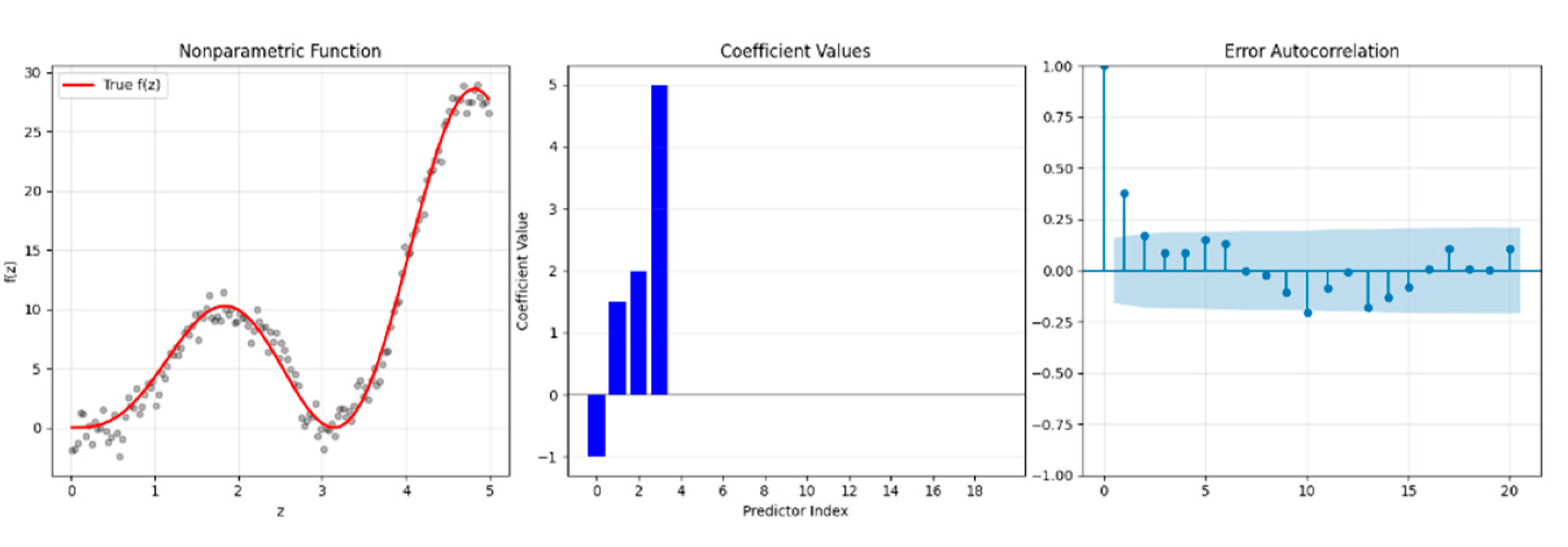
Figure 5.
Autocorrelation functions (acf) for the model error in (5.3): Panel (a) acf plot of original response variable; panel (b) acf plot for difference of the
Figure 5.
Autocorrelation functions (acf) for the model error in (5.3): Panel (a) acf plot of original response variable; panel (b) acf plot for difference of the
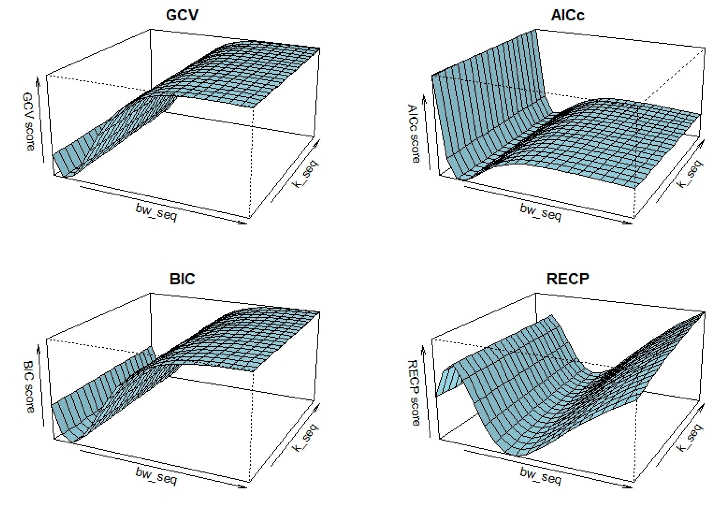
Figure 6.
Informative plots for the Airline Delay dataset.
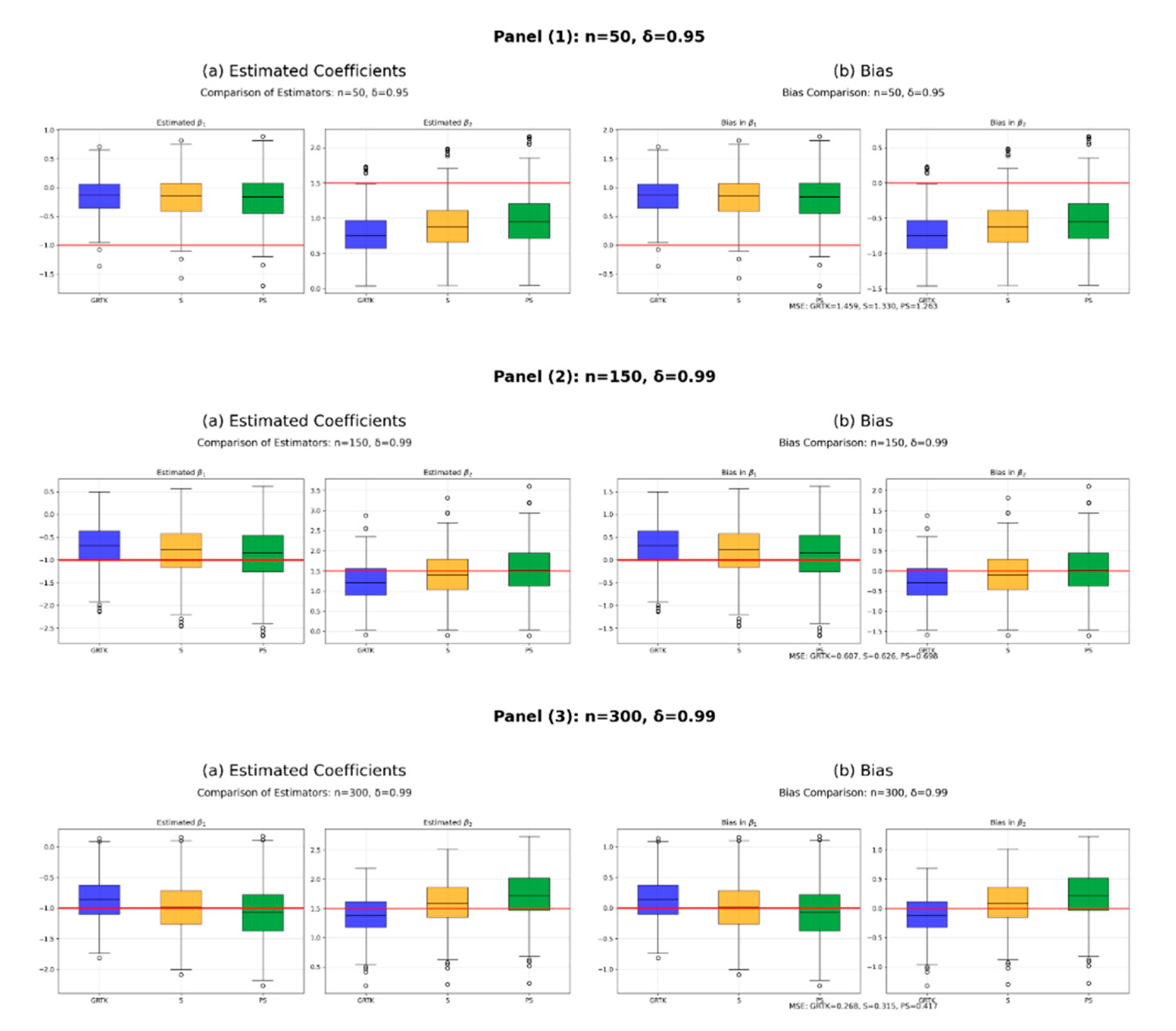
Figure 7.
Selection of
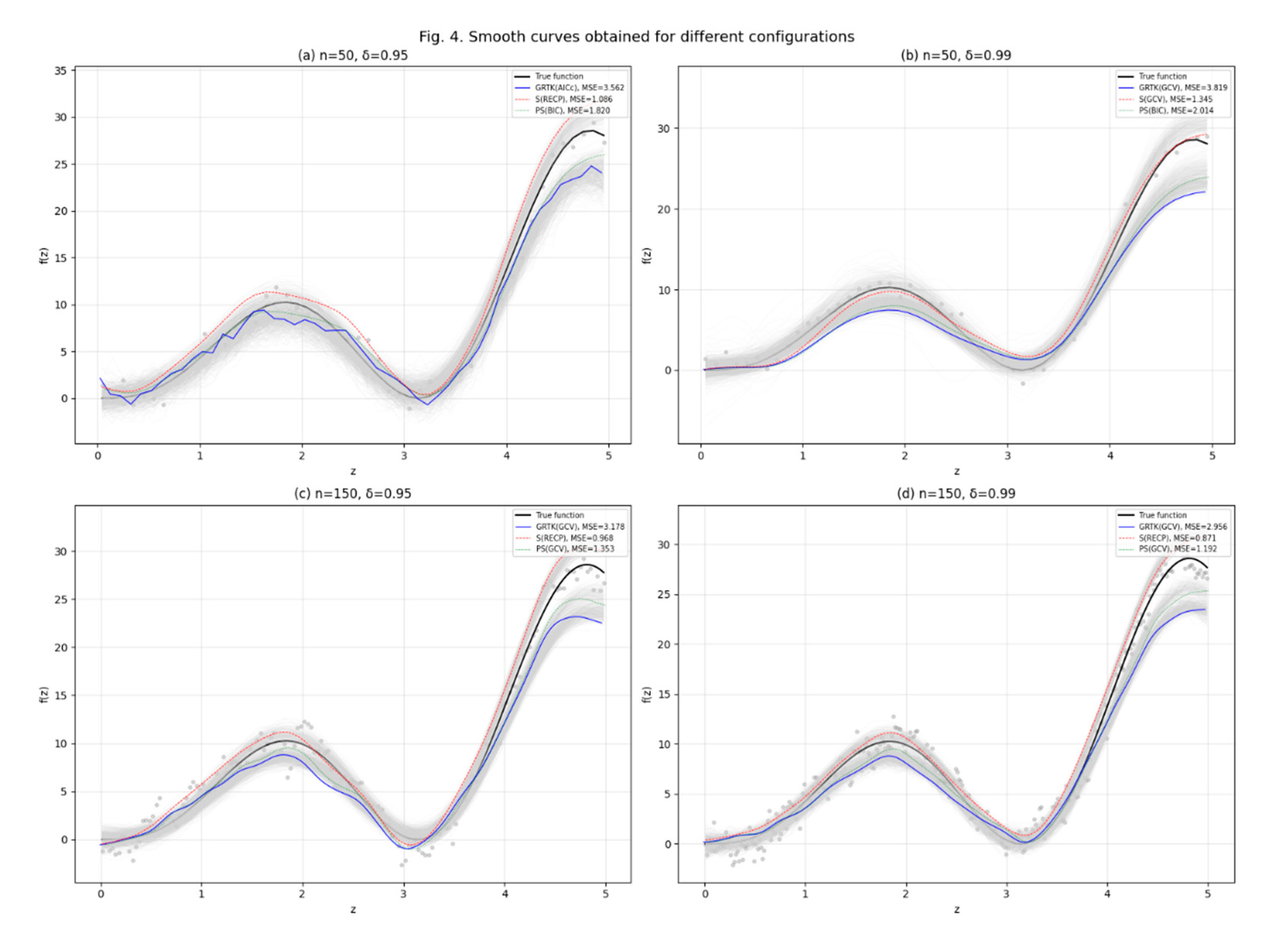
Figure 8.
Residual analysis for the airline delay dataset. In the plots at the top of the figure show the acf plots of residuals obtained for the estimated models based on the corresponding criterion. The plots at the bottom show the scatterplots of the residuals around
Figure 8.
Residual analysis for the airline delay dataset. In the plots at the top of the figure show the acf plots of residuals obtained for the estimated models based on the corresponding criterion. The plots at the bottom show the scatterplots of the residuals around
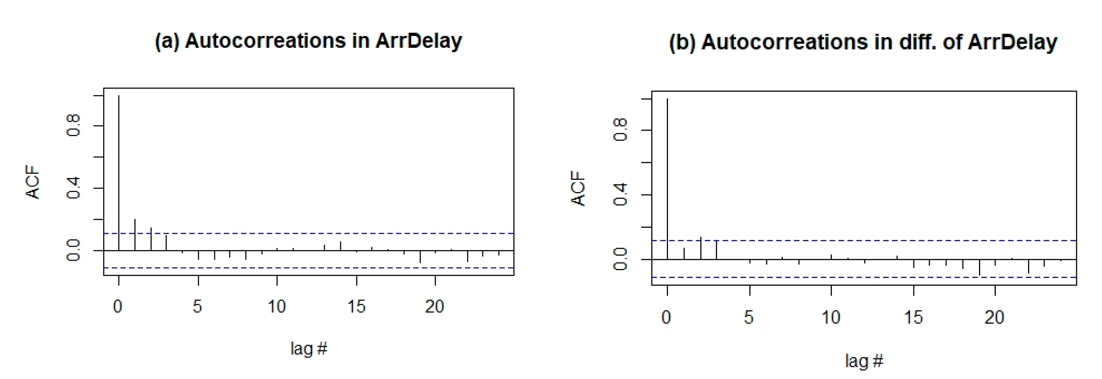
Figure 2.
Selection of
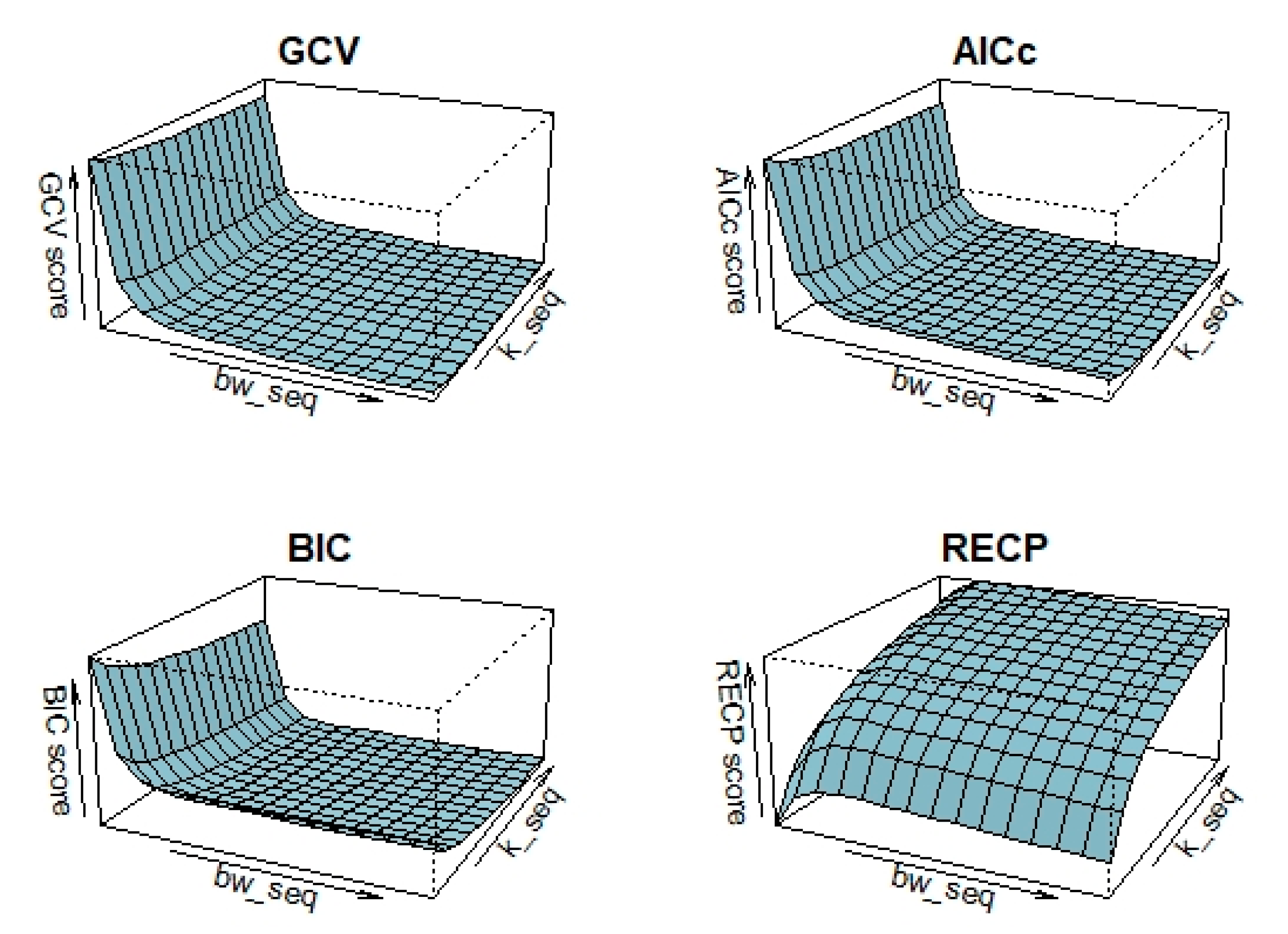
Figure 4.
Smooth curves obtained for different configurations to show effect of the correlation level
Figure 4.
Smooth curves obtained for different configurations to show effect of the correlation level
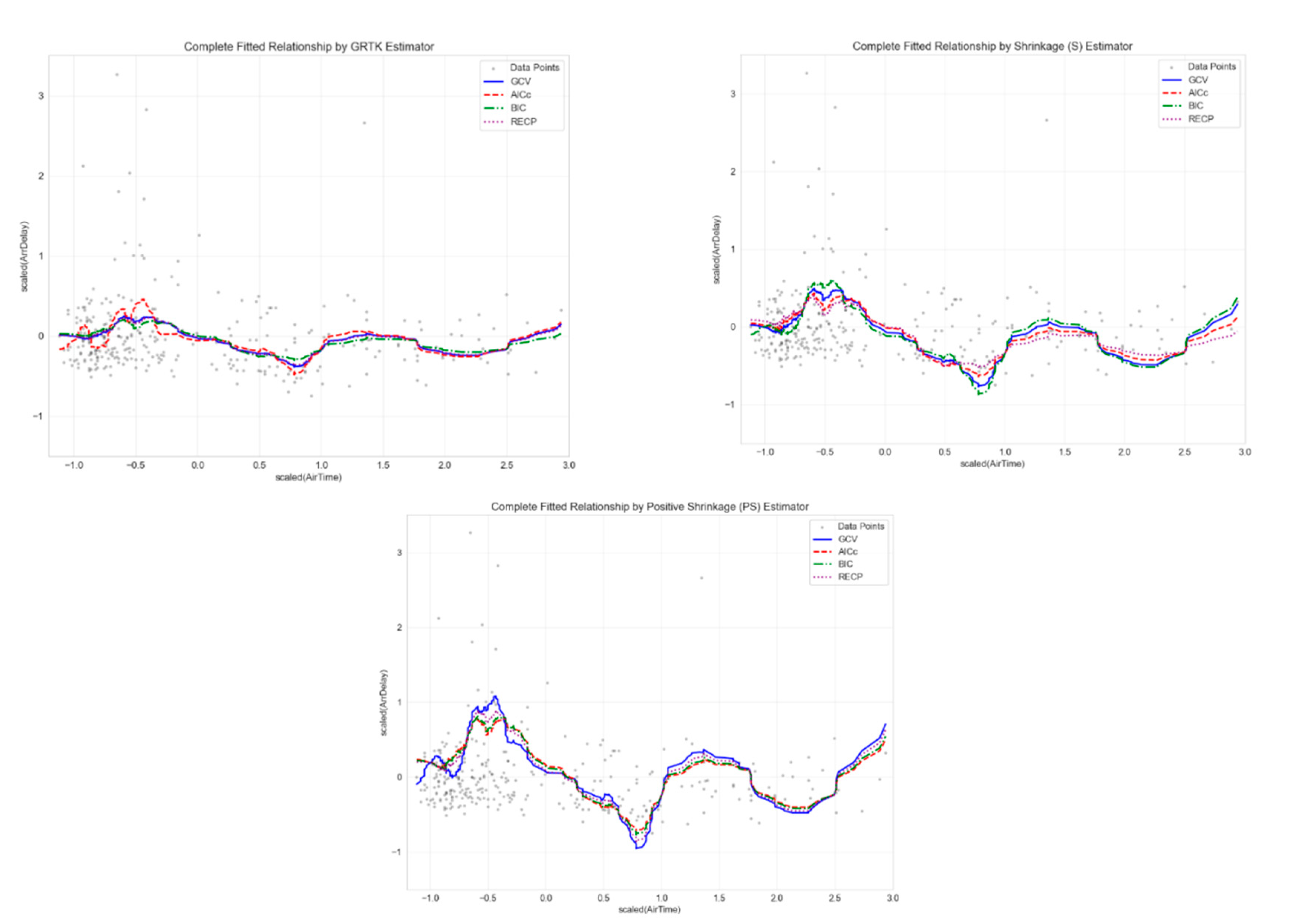
Table 1.
Optimal
Table 2.
Outcomes of simulations with bias, variance and SMSD scores for
Table 4.
Outcomes of simulations with bias, variance and SMSD scores for.
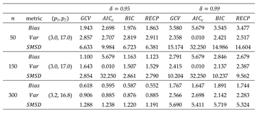 |
Table 5.
MSE values for the estimated nonparametric component f ̂_GRTK for all simulation combinations.
Table 5.
MSE values for the estimated nonparametric component f ̂_GRTK for all simulation combinations.
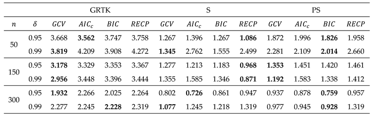 |
Table 6.
Performance of the GRTK estimators for parametric and nonparametric components of the model.
Table 6.
Performance of the GRTK estimators for parametric and nonparametric components of the model.
| Measure/Criterion | ||||
| 0.952 | 0.953 | 0.953 | 0.965 | |
| 0.932 | 0.936 | 0.936 | 0.935 | |
| 0.270 | 0.246 | 0.246 | 0.31 | |
| 0.712 | 0.809 | 0.741 | 0.825 | |
| 0.821 | 0.836 | 0.831 | 0.857 | |
| 0.210 | 0.225 | 0.226 | 0.280 | |
| 0.705 | 0.713 | 0.673 | 0.711 | |
| 0.735 | 0.736 | 0.735 | 0.735 | |
| 0.172 | 0.211 | 0.183 | 0.191 |
Disclaimer/Publisher’s Note: The statements, opinions and data contained in all publications are solely those of the individual author(s) and contributor(s) and not of MDPI and/or the editor(s). MDPI and/or the editor(s) disclaim responsibility for any injury to people or property resulting from any ideas, methods, instructions or products referred to in the content. |
© 2025 by the authors. Licensee MDPI, Basel, Switzerland. This article is an open access article distributed under the terms and conditions of the Creative Commons Attribution (CC BY) license (http://creativecommons.org/licenses/by/4.0/).
Copyright: This open access article is published under a Creative Commons CC BY 4.0 license, which permit the free download, distribution, and reuse, provided that the author and preprint are cited in any reuse.


