
Submitted:
06 October 2025
Posted:
07 October 2025
You are already at the latest version
Abstract
Artificial neural networks (ANNs) achieve remarkable performance but at the unsustainable cost of extreme parameter density. In contrast, biological networks operate with ultra-sparse, highly organized structures, where dendrites play a central role in shaping information integration. Here we introduce the Dendritic Network Model (DNM), a generative framework that bridges this gap by embedding dendritic-inspired connectivity principles into sparse artificial networks. Unlike conventional random initialization, DNM defines connectivity through parametric distributions of dendrites, receptive fields, and synapses, enabling precise control of modularity, hierarchy, and degree heterogeneity. This parametric flexibility allows DNM to generate a wide spectrum of network topologies, from clustered modular architectures to scale-free hierarchies, whose geometry can be characterized and optimized with network-science metrics. Across image classification benchmarks (MNIST, Fashion-MNIST, EMNIST, CIFAR-10), DNM consistently outperforms classical sparse initializations at extreme sparsity (99\%), in both static and dynamic sparse training regimes. Moreover, when integrated into state-of-the-art dynamic sparse training frameworks and applied to Transformer architectures for machine translation, DNM enhances accuracy while preserving efficiency. By aligning neural network initialization with dendritic design principles, DNM demonstrates that sparse bio-inspired network science modelling is a structural advantage in deep learning, offering a principled initialization framework to train scalable and energy-efficient machine intelligence.
Keywords:
artificial intelligence
; dynamic sparse training
; brain network science
; network topology
1. Introduction
Artificial neural networks (ANNs) have demonstrated remarkable potential in various fields; however, their size, often comprising billions of parameters, poses challenges for both economic viability and environmental sustainability. Biological neural networks, in contrast, can efficiently process information using ultra-sparse structures [1,2]. This efficiency arises from the brain’s highly structured and evolutionarily optimized network topology. A central component of this architecture is the dendritic tree, the primary receptive surface of the neuron [3]. Conventional ANNs omit a crucial component of the brain’s efficiency since they traditionally depict neurons as simple point-like integrators, mainly ignoring the computing power inherent in the intricate structure of dendrites.
Research has revealed that dendrites are not passive conductors but active computational units capable of performing sophisticated, nonlinear operations [4,5]. This insight has motivated theoretical frameworks that model a single neuron as a multi-layer network, where dendritic branches act as nonlinear subunits that feed a final integrator at the cell body [6,7]. The model proposed by Poirazi and colleagues, which focuses on non-linear dendritic computation and is conceptually similar to a convolutional model, has been shown to enhance the storage capacity and learning speed of neuron models [7]. Subsequent efforts to translate these principles into artificial systems have identified that dendritic morphology has a significant impact on performance [8,9,10]. These approaches, however, are often limited to fixed structures that mimic the computational non-linearity or direct morphology of biological neurons. Therefore, we identify a critical gap in the field: the lack of a flexible, principled framework for generating and testing dendritic topologies.
To address this, we introduce a dendritic-inspired network science generative model for sparse topology design of neural networks: the Dendritic Network Model (DNM). The novelty of our model lies in the topological organization of the receptive fields on the input layers. Rather than modeling non-linear dendritic computation, we introduce a network science topological initialization model. The DNM is a flexible generative model for creating sparse, biologically-inspired network architectures, constructing a network topology grounded in connectivity principles rather than direct morphological imitation. The model’s parametric approach enables the systematic exploration of the relationship between network structure and computational function. The DNM provides a principled method for generating sparse network initializations that can be integrated into modern deep learning frameworks. We demonstrate that this approach can improve performance over standard sparse initialization techniques and offers a powerful platform for exploring how structural constraints, inspired by biology, can lead to more efficient and capable artificial neural networks.
First, we describe the Dendritic Network Model in detail and analyse its topology and geometric characterization. We evaluate its effectiveness with extensive experiments across multiple architectures and tasks. To assess its basic functionality, we use it to initialize several static and dynamic sparse training (DST) methods on MLPs for image classification on the MNIST [11], EMNIST [12], Fashion MNIST [13], and CIFAR-10 [14] datasets. The results show that DNM clearly outperforms other sparse initialization methods over all training models tested at 99% sparsity. Next, we extend the tests on Transformers [15] for Machine Translation on the Multi30k en-de [16], IWSLT14 en-de [17], and WMT17 en-de [18] benchmarks. On this architecture, DNM outperforms all topological initialization methods at high sparsity levels. These findings underscore the potential of DNM in enabling highly efficient and effective network initialization for large-scale sparse neural network training. By analyzing the best-performing DNM topologies, we can also gain insights into the relationship between network geometry, data structure, and model performance.
2. Related Works
2.1. Sparse Topological Initialization Methods
Dynamic sparse training (DST) trains a neural network with a sparse topology that evolves throughout the learning process. The initial arrangement of the connections is a critical aspect of this framework. This starting structure determines the initial pathways for information flow and acts as the foundational scaffold upon which the network learns and evolves. A well-designed initial topology can significantly improve a model’s final performance and training efficiency, whereas a poor starting point can severely hinder its ability to learn effectively. The principal topological initialization approaches for dynamic sparse training are grounded in network science theory, where three basic generative models for monopartite sparse artificial complex networks are the Erdős-Rényi (ER) model [19], the Watts-Strogatz (WS) model [20], and the Barabási-Albert (BA) model [21]. Since the standard WS and BA models are not directly designed for bipartite networks, they were recently extended into their bipartite counterparts and termed as Bipartite Small-World (BSW) and Bipartite Scale-Free (BSF) [22], respectively. BSW generally outperforms BSF for dynamic sparse training [22]. The Correlated Sparse Topological Initialization (CSTI) [23] is a feature-informed topological initialization method that considers the links with the strongest Pearson correlations between nodes and features in the input layer. SNIP [24] is a data-informed pruning method that identifies important connections based on their saliency scores, calculated using the gradients of the loss function with respect to the weights. Ramanujan graphs [25] are a class of sparse graphs that exhibit optimal spectral properties, making them suitable for initializing neural networks with desirable connectivity patterns. The Bipartite Receptive Field (BRF) network model [26] generates networks with brain-like receptive field connectivity. This is the first attempt to mimic the structure of brain connections in a sparse network initialization model.
3. The Dendritic Network Model
3.1. Biological Inspiration and Principles
The architecture of the Dendritic Network Model (DNM) is inspired by the structure of biological neurons. In the nervous system, neurons process information through complex, branching extensions called dendrites, which act as the primary receivers of synaptic signals. Inspired by this phenomenon, the DNM shapes each sandwich layer (a bipartite subnetwork that links the input nodes of a layer to their output nodes) in a way that output neurons are connected to distinct groups of input neurons with multiple dendritic branches (Figure 1). In the DNM, an output neuron’s connections are organized into distinct clusters called dendrites. Each branch connects the output neuron to a consecutive batch of input neurons. These connected blocks are separated by "inactive spaces", which are groups of input neurons that remain unconnected to that specific output neuron. All of an output neuron’s branches must be formed within a localized receptive window, a predefined segment of the input layer. This method results in a structured and clustered connectivity pattern, moving away from random, unstructured sparsity.
3.2. Parametric Specification
By parametrizing the core biological features of DNM, like the number of dendrites for each output neuron, the size of the receptive windows, the distribution of synapses across dendrites, and the degree distribution across output neurons, the DNM provides a flexible framework for generating network topologies that are sparse, structured, and biologically plausible. Figure A1 shows how the connectivity of an MLP is shaped by the DNM.
Sparsity (s)
The sparsity parameter (s) defines the percentage of potential connections between the input and output layers that are absent, controlling the trade-off between computational cost and representational power.
Dendritic Distribution
The dendritic distribution governs the number of branches that connect each output neuron to the input layer, which can be seen as the number of distinct input regions a neuron integrates information from. The central parameter for this is M, which defines the mean number of dendrites per output neuron. This distribution can be implemented in one of three ways. The simplest is a fixed distribution, where every output neuron has exactly M dendrites. Alternatively, a non-spatial distribution introduces stochasticity by sampling the number of dendrites for each output neuron from a probability distribution (e.g., Gaussian or uniform) with a mean of M. Finally, a spatial distribution makes the number of dendrites for each neuron dependent on its position within the layer. Using a Gaussian or inverted Gaussian profile, this configuration implies that some neurons integrate signals from many distinct input regions (a high dendrite count), while others connect to fewer, more focused regions (a low dendrite count).
Receptive Field Width Distribution
The receptive field width distribution determines the size of the receptive field for each output neuron, mirroring the concept of receptive fields in biology. This process is governed by a mean parameter, , which specifies the average percentage of consecutive input neurons on the input layer from which an output neuron can sample connections. This distribution can be configured in several ways: a fixed distribution assigns an identical window size to all output neurons; a non-spatial distribution introduces variability by drawing each neuron’s window size from a probability distribution (e.g., Gaussian or uniform) centered on ; and a spatial distribution links the window size to the neuron’s position in its layer, allowing for configurations where receptive windows are, for instance, wider at the center and narrower at the edges.
Degree Distribution
The degree distribution samples the number of incoming connections for each output neuron. This can be configured using a fixed distribution, where every output neuron is allocated the same degree. To introduce heterogeneity, a non-spatial distribution can be used to sample the degree for each neuron from a probability distribution. Finally, a spatial distribution allows the degree to vary based on the neuron’s position, for instance, by creating highly connected, hub-like neurons at the center of the layer. The mean degree is set by the layer size and target sparsity.
Synaptic Distribution
Once an output neuron’s total degree is determined, the synaptic distribution allocates these connections among its various dendritic branches. The allocation can be fixed, where each dendrite receives an equal number of synapses. Alternatively, a non-spatial distribution can introduce random variability in synapse counts per dendrite. A spatial distribution can also be applied, making the number of synapses dependent on a dendrite’s topological location, for example by assigning more connections to central branches versus outer ones. This distribution has a mean of , where is the size of the input layer.
Layer Border Wiring Pattern
The DNM includes a setting to control how connections are handled at the boundaries of the input layer. The default behavior is a wrap-around topology, where the input layer is treated as a ring. This means a receptive window for a neuron near one edge can wrap around to connect to neurons on the opposite edge, ensuring all neurons have a similarly structured receptive field. Alternatively, a bounded pattern can be enforced. In this mode, receptive windows are strictly confined within the layer’s physical boundaries. If a receptive field extends beyond the first or last input neuron, it is clamped to the edge. This enforces a more stringent locality, which we analyze further in Appendix H.
3.3. Network Topology and Geometric Characterization
The parametric nature of the DNM allows for the generation of a vast landscape of network topologies.1 In this section, we explore this landscape by systematically varying the model’s key hyperparameters and analyzing the resulting structural changes. We employ both visual analysis and quantitative measures grounded in network science to provide a comprehensive geometric characterization of the generated networks.
Figure 2 illustrates this topological diversity by comparing a baseline random network with several DNM configurations in a 3-layered MLP of dimensions , with sparsity. Each panel displays the network’s coalescent embedding [27] in hyperbolic space, its adjacency matrix, and a direct bipartite graph representation, alongside key network science metrics: characteristic path length (L), modularity (Q), structural consistency (), and the power-law exponent of the degree distribution (). The coalescent embedding method and the metrics adopted are detailed in Appendix A. The baseline random network (Figure 2a) exhibits a lack of clear structure, which is quantified by low modularity and structural consistency (, ). The high value of and the uniform scattering of nodes in the hyperbolic embedding confirm the absence of any scale-free organization. Figure 2b represents a DNM network with , , and all distributions fixed. This model generates highly structured and modular networks, as evidenced by the high modularity () and structural consistency (). Similar measures are found when setting a spatial Gaussian synaptic distribution (Figure 2d, , ), because this configuration does not alter the structure of the network much, as highlighted by the adjacency matrix depicted. A key finding is that by setting a spatial Gaussian degree distribution (Figure 2c), the DNM generates a hierarchical structure. Indeed, the power law exponent yielded () falls within the typical range for scale-free networks (). This property is clearly evidenced by the emergence of a tree-like structure in the hyperbolic embedding.
This analysis shows that DNM is a highly flexible framework that can produce a wide spectrum of network architectures. This ability to controllably generate diverse network geometries is fundamental for analyzing the relationship between network structure and computational function in ANNs.
4. Experiments
4.1. Experimental Setup
To test the basic advantage of DNM over other initialization methods, we evaluate it for static sparse training using MLPs for image classification tasks on the MNIST [11], Fashion MNIST [13], EMNIST [12], and CIFAR10 [14] datasets. To further validate our approach, we replicate the tests on CHTs [26] and CHTss, which are the state-of-the-art dynamic sparse training (DST) methods. We use the SET [28] and RigL [29] dynamic sparse training methods as baselines. Finally, we test DNM for initialization of the CHTs and CHTss methods, on Transformers for machine translation tasks on the Multi30k en-de [16], IWSLT14 en-de [30], and WMT17 [18] datasets. For MLP training, we sparsify all layers except the final layer, as it would lead to disconnected output neurons, and connections in the final layer are relatively fewer compared to the previous layers. For Transformers, we apply DST to all linear layers, excluding the embedding and final generator layer. The hyperparameter settings of the experiments are detailed in Appendix B. Furthermore, we conduct a series of sensitivity tests on the hyperparameters of the DNM in Appendix C.
Baseline methods
We compare the DNM network with the baseline approaches in the literature. On static sparse training, we compare DNM with a randomly initialized network, the Bipartite Small World (BSW) [22], the Bipartite Receptive Field (BRF) [26], and the Ramanujan graph [25] initialization techniques. We use CSTI [23] and SNIP [24] as the baseline models, although this comparison is inherently unfair due to their data-informed nature. For dynamic sparse training, we compare DNM with a random initialization, BRF, BSW, Ramanujan graph, SNIP and CSTI. Finally, for tests on Transformer models, we compare DNM with the BRF initialization.
4.2. MLP for Image Classification
Static sparse training
As an initial evaluation of DNM’s performance, we compare it to other topological initialization methods for static sparse training for image classification tasks. On all benchmarks, DNM outperforms the baseline models, as shown in Table 1. Analyzing the best-performing DNM networks is crucial to understanding the relationship between network topology and task performance. This aspect is assessed in Section 5.
Dynamic sparse training
We first test DNM on the baseline dynamic sparse training methods, SET and RigL. As shown in Table 2 and Table 3, DNM outperforms the other sparse initialization methods of MLPs (99% sparsity) over all the datasets tested. The model’s performance is comparable to the input-informed CSTI and SNIP, highlighting that DNM’s high degree of freedom can match a topology induced by data features.
4.3. Transformer for Machine Translation
We assess the Transformer’s performance on a machine translation task across three datasets. We take the best performance of the model on the validation set and report the BLEU score on the test set. Beam search, with a beam size of 2, is employed to optimize the evaluation process. On the Multi30k and IWSLT datasets, we conduct a thorough hyperparameter search to find the best settings for our DNM model. For the WMT dataset, in contrast, we simply use the best settings found in the previous tests. This approach helps to verify that DNM performs well even without extensive, dataset-specific tuning. DNM markedly improves the performance of the CHTs algorithm (Table 6 and Table 7). However, its impact on CHTss is similar to the BRF baseline. This is expected, as CHTss’s gradual decay mechanism starts from a dense 50% state, where the initial network structure is less critical and the topological advantages of DNM are less pronounced. In Appendix G, we prove this by showing the effect of different initial sparsity levels on the performance of DNM.
5. Results Analysis
To understand which network structures are inherently best suited for specific tasks, we analyze the topologies of the top-performing models from our static sparse training experiments. Static sparse training is ideal for this analysis because its fixed topology allows us to link network structure to task performance directly, isolating it as a variable in a way that is impossible with dynamic methods. Figure 3 shows the adjacency matrices of these models, their direct bipartite graph representations, and their key metrics in network science. For image classification on MNIST and Fashion MNIST, the optimal network’s topology is identical. This network is scale-free () and exhibits a small characteristic path. Also on EMNIST, the best performing network exhibits a power-law degree distribution. Finally, we obtain contrasting results when assessing the network adopted for CIFAR-10 classification. Its high parameter indicates that this network lacks hub nodes, possibly hinting that for more complex datasets like CIFAR-10, a more distributed and less hierarchical connectivity pattern is advantageous. Such a topology might promote the parallel processing of localized features across the input space, which is critical for natural image recognition, where object location and context vary significantly. Appendix C gives a more detailed analysis of the best parameter combinations for each of the tests performed.
Overall, this analysis reveals a compelling relationship between task complexity and optimal network topology. While simpler, more structured datasets like MNIST and EMNIST benefit from scale-free, hierarchical architectures that can efficiently integrate global features through hub neurons, the more complex CIFAR-10 dataset favors a flatter, more distributed architecture. This underscores the potential of the DNM: its parametric flexibility allows it to generate these distinct, task-optimized topologies, moving beyond a one-size-fits-all approach to sparse initialization.
6. Conclusions
In this work, we introduced the Dendritic Network Model (DNM), a novel generative framework for initializing sparse neural networks inspired by the structure of biological dendrites. We have shown that the DNM is a highly flexible tool capable of producing a wide spectrum of network architectures, from modular to hierarchical and scale-free, by systematically adjusting its core parameters.
Our extensive experiments across multiple architectures demonstrate the effectiveness of our approach. At extreme sparsity levels, DNM consistently outperforms alternative topological initialization methods in both static and dynamic sparse training regimes, sometimes exceeding the performance of the data-informed CSTI and SNIP.
Crucially, our studies reveal a compelling link between network topology and task complexity. While simpler datasets benefit from hierarchical, scale-free structures, more complex visual data favors distributed, non-hierarchical connectivity. This finding underscores that the optimal sparse topology is task-dependent and highlights the power of DNM as a principled platform for exploring the relationship between network geometry and function.
Figure A1.
Representations of the network’s topology obtained by varying a DNM parameter while keeping all others fixed.
Figure A1.
Representations of the network’s topology obtained by varying a DNM parameter while keeping all others fixed.
Figure A2.
Representations of the network’s topology obtained by varying a DNM parameter while keeping all others fixed.
Figure A2.
Representations of the network’s topology obtained by varying a DNM parameter while keeping all others fixed.
Appendix A. Glossary of Network Science
In this section, we introduce the basic notions of network science mentioned in this article.
Scale-Free Network
A Scale-Free Network [21] is characterized by a highly uneven distribution of degrees amongst the nodes. A small number of nodes, called hubs, have a very high degree, and a large number of nodes have very few connections. The degree distribution of scale-free networks follows a power law trend , where is a constant smaller than 3. In contrast, nodes in random networks are distributed following a Binomial distribution.
Watts-Strogatz Model and Small-World Network
A Small-World Network [20] is characterized by a small average path length. This property implies that any two nodes can communicate through a short chain of connections. The Watts-Strogatz [20] model is well known for its high clustering and short path lengths. This network is modelled by a parameter between 0 and 1 that can determine its level of clustering. When takes low values (), the WS network is a highly clustered lattice. On the other hand, when approaches 1, the network becomes a random small-world graph. Intermediate values of can generate a clustered network that maintains small-world connectivity.
Formally, a network is small-world when the path of length L between two randomly chosen nodes grows proportionally to the logarithm of the number of nodes (N) in the network, that is:
Structural Consistency
Structural consistency [31] is an index based on the first-order matrix perturbation of the adjacency matrix, which represents the predictability of the network structure. A perturbation set is randomly sampled from the original link set E. Identifying as the links ranked as the top L according to the structural perturbation method [31], with , the structural consistency is calculated as:
Modularity
Modularity [32] quantifies the tendency of nodes in the network to form distinct communities (or clusters). This measure ranges from -1 to 1. A high modularity score (close to 1) hints at the presence of dense connections between nodes within communities, but sparse connections between nodes belonging to different communities. A modularity score close to 0, in contrast, suggests that the network lacks any community organization and the interaction between nodes is essentially uniform. When modularity approaches -1, the network exhibits an anticommunity structure. This means that nodes are strongly connected across the network, and there is little differentiation into separate groups. In other words, a negative modularity represents a cohesive network. The formula to compute the modularity (Q) is:
where A represents the network’s adjacency matrix, and and are the degrees of nodes i and j, respectively. is the Kronecker delta function, which equals one if i and j are in the same community, else it equals 0.
Characteristic path length
The characteristic path length is computed as the average node-pairs length in the network; it is a measure associated with the network’s small-worldness [33]. The characteristic path length (L) is derived by:
where n is the number of nodes in the network, and d(i,j) is the shortest path length between node i and node j.
Coalescent Embedding
Coalescent embedding [34] is a class of machine learning algorithms used for unsupervised dimensionality reduction and embedding complex networks in a geometric space, often hyperbolic. This method maps high-dimensional information on a low-dimensional embedding while maintaining the essential topological features of the network. This embedding reveals latent structures of the system, like hierarchical and scale-free structures. In this article, coalescent embedding maps the networks that have latent hyperbolic geometry onto the two-dimensional hyperbolic space. The approach involves 4 steps: 1) links are pre-weighted with topological rules that approximate the underlying network geometry [33]; 2) non-linear dimensionality reduction; 3) generation of angular coordinates; 4) generation of radial coordinates.
This process is illustrated in Figure 2, which showcases the results of applying a specific coalescent embedding pipeline to four different synthetic networks. The embeddings shown were generated without any initial link pre-weighting (step 1). For the non-linear dimensionality reduction (step 2), the Isomap [35] algorithm was used. Finally, the angular coordinates (step 3) were determined using Equidistant Adjustment (EA), a process that preserves the relative order of the nodes while arranging them at perfectly uniform angular intervals.
Appendix B. Hyperparameter Settings and Implementation Details
Our experimental setup is designed to replicate the conditions in [26]. Configurations are assessed on validation sets before being tested on separate test sets. All reported scores are the average of three runs using different random seeds, presented with their corresponding standard errors.
Appendix B.1. MLP for Image Classification
Models are trained for 100 epochs using Stochastic Gradient Descent (SGD) with a learning rate of 0.025, a batch size of 32, and a weight decay of . All sparse models are trained at a 99% sparsity level. For dynamic methods, we used SET, RigL, CHTs and CHTss. The regrowth strategy for CHTs and CHTss is CH2_L3n [36]. The CHTss model begins with an initial sparsity of 50% and gradually increases to the final 99% target using an s-shaped scheduler. For our DNM, we conduct a grid search over its key hyperparameters. We tested a mean dendrite count (M) of 3, 7, and 21. For the dendritic, degree, receptive field width, and synaptic distributions, we searched across fixed, spatial Gaussian, and spatial inverted Gaussian options. The mean receptive field width () was fixed at 1.0. For the BSW baseline, the rewiring probability is searched in the set {0.0, 0.2, 0.4, 0.6, 0.8, 1.0}. For the BRF baseline, we searched the randomness parameter r over the same set of values, and also tested both fixed and uniform degree distributions.
Appendix B.2. Transformer for Machine Translation
We use a standard 6-layer Transformer architecture with 8 attention heads and a model dimension of 512. The dimension of the feed-forward network is set to 1024 for Multi30k and 2048 for IWSLT14 and WMT17. All models are trained using the Adam optimizer [37] with the noam learning rate schedule. Dataset-specific training parameters are as follows:
- Multi30k: Trained for 5,000 steps with a learning rate of 0.25, 1000 warmup steps, and a batch size of 1024.
- IWSLT14: Trained for 20,000 steps with a learning rate of 2.0, 6000 warmup steps, and a batch size of 10240.
- WMT17: Trained for 80,000 steps with a learning rate of 2.0, 8000 warmup steps, and a batch size of 12000.
We evaluated models at final sparsity levels of 90% and 95%. The CHTss models started from a denser state (50% sparsity) and decayed to the target sparsity. For Multi30k and IWSLT14, we performed a comprehensive hyperparameter search. The search for IWSLT14 included a mean dendrite count and various combinations of fixed and spatial distributions for all DNM parameters. For WMT17, to assess generalization, we did not perform a new search. Instead, we directly applied the best-performing DNM configuration identified from the IWSLT14 experiments. This configuration used M=7 with a fixed dendritic distribution, alongside spatial Gaussian or inverse-Gaussian distributions for degree, receptive field width, and synapses.
Appendix C. Sensitivity Tests
We provide sensitivity tests for DNM hyperparameters. First, we focus on the analysis of CHTs and CHTss on MLPs for image classification at 99% sparsity. Next, we study the parametric configurations for the CHTs and CHTss model on the Multi30k translation task at 90% sparsity. For each task, we vary one parameter at a time, keeping the others fixed to a specific configuration. We calculate the coefficient of variation (CV) of the scores to quantify the sensitivity of the model to each parameter. A low CV indicates that the model’s performance is relatively stable across different settings of that parameter, suggesting low sensitivity. Conversely, a high CV suggests that the model’s performance is more variable and sensitive to changes in that parameter. We average each parameter’s CV across various parametric configurations to obtain a robust measure of sensitivity. Next, we analyse the top 5% best-performing configurations for each task to understand the commonalities in the optimal settings. This method not only helps us understand which parameters are most influential but also guides future configurations for similar tasks.
Dynamic Sparse Training for Image Classification
We analyse the sensitivity of DNM parameters for the initialization of CHTs and CHTss models on MLPs for image classification at 99% sparsity. The analysis is performed over MNIST, Fashion MNIST, EMNIST, and CIFAR-10. The sensitivity analysis, summarized in Table A1, evaluates the impact of DNM initialization parameters for CHTs and CHTss models at 99% sparsity. A key finding is the significantly heightened sensitivity of the CHTss model compared to CHTs, a disparity that amplifies with increasing dataset complexity from MNIST to CIFAR-10. Across all benchmarks, the Degree Distribution consistently emerges as the most critical parameter, highlighting the paramount importance of initial network connectivity. Following in descending order of influence are the Receptive Field Width, Dendritic, and Synaptic distributions. These results underscore that while both architectures show similar robustness on simpler tasks, the effective deployment of the CHTss model on more challenging problems is critically dependent on the precise calibration of its initial topological structure. Analyzing the top 5% best-performing configurations, we observe similar trends across various datasets (Figure A3). The most relevant findings is that a spatial gaussian receptive field width distribution is constantly preferred.
Figure A3.
Sensitivity analysis of the DNM parameters for CHTs initialization over MLPs for image classification on CIFAR-10 at 99% sparsity.
Figure A3.
Sensitivity analysis of the DNM parameters for CHTs initialization over MLPs for image classification on CIFAR-10 at 99% sparsity.

Table A1.
Sensitivity Analysis Results for CHTs and CHTss on MNIST, EMNIST, Fashion MNIST, CIFAR-10 for Image Classification. The table presents the average coefficient of variation (CV) for each DNM parameter across different configurations at 99% sparsity level. A higher CV indicates greater sensitivity of the model’s performance to changes in that parameter.
| MNIST | EMNIST | Fashion MNIST | CIFAR-10 | |||||
|---|---|---|---|---|---|---|---|---|
| Parameter | CHTs | CHTss | CHTs | CHTss | CHTs | CHTss | CHTs | CHTss |
| Degree Dist | 0.001538 | 0.001538 | 0.001419 | 0.009172 | 0.003379 | 0.017639 | 0.017639 | 0.017639 |
| Rec Field Width Dist | 0.000506 | 0.000506 | 0.001585 | 0.006154 | 0.001205 | 0.005381 | 0.005381 | 0.005381 |
| Dendritic Dist | 0.000525 | 0.000525 | 0.001265 | 0.003620 | 0.001136 | 0.004983 | 0.004983 | 0.004983 |
| Synaptic Dist | 0.000464 | 0.000464 | 0.000989 | 0.002538 | 0.000964 | 0.004306 | 0.004306 | 0.004306 |
Dynamic Sparse Training for Machine Translation
We focus on the analysis of DNM for the initialization of the CHTss model on Multi-30k for machine translation. Both at 90% and 95% sparsity, the calculated coefficients of variation do not surpass 0.01. This indicates that the model’s performance is relatively stable across different settings of each parameter, suggesting low sensitivity (Table A2). At both sparsity levels, the dendritic distribution appears to be the most sensitive, whereas M and are the most stable. Analyzing the top 5% best-performing configurations, we observe that spatial distributions generally outperform fixed distributions (Figure A4).
Table A2.
Sensitivity Analysis Results for CHTss on Multi30k for Machine Translation. The table presents the average coefficient of variation (CV) for each DNM parameter across different configurations at 90% and 95% sparsity levels. A higher CV indicates greater sensitivity of the model’s performance to changes in that parameter.
| Parameter | Average Coefficient of Variation (CV) | |
|---|---|---|
| 90% | 95% | |
| Dendritic distribution | 0.010643 | 0.009340 |
| Degree distribution | 0.010270 | 0.008436 |
| Receptive Field Width Distribution | 0.009830 | 0.009103 |
| Synaptic distribution | 0.009663 | 0.009310 |
| M | 0.008959 | 0.007806 |
| 0.008210 | 0.007461 | |
| Note: Higher CV indicates greater impact on performance. | ||
Figure A4.
Sensitivity analysis of the DNM parameters for CHTss initialization over Transformer models for machine translation on Multi30k at 90% sparsity.
Figure A4.
Sensitivity analysis of the DNM parameters for CHTss initialization over Transformer models for machine translation on Multi30k at 90% sparsity.
Appendix D. Modelling Dendritic Networks
The Dendritic Network Model (DNM) generates the sparse connectivity matrix of sandwich layers by iteratively building connections for each output neuron based on the principles of dendritic branching and localized receptive fields. The generation process can be broken down into the following steps:
- Determine the degree of each output neuron in the layer based on one of the three distribution strategies (fixed, non-spatial, spatial). A probabilistic rounding and adjustment mechanism ensures that no output neuron is disconnected and the sampled degrees sum precisely to the target total number of connections of the layer.
- Next, for each output neuron j, define a receptive field. This is done by topologically mapping the output neuron’s position at a central point in the input layer and establishing a receptive window around this center. The size of this window is controlled by the parameter , which determines the fraction of the input layer that the neuron can connect to. itself can be fixed or sampled from a spatial or non-spatial distribution.
- For each output neuron, determine the number of dendritic branches, to be used to connect it to the input layer. Again, is determined based on one of the three configurations (fixed for all neurons, or sampled from a distribution that could depend on the neuron’s position in the layer).
- Place the dendrites as dendritic centers within the neuron’s receptive window, spacing them evenly across the window.
- The neuron’s total degree, obtained from step 1, is distributed across its dendrites according to a synaptic distribution (fixed, spatial, or non-spatial). For each dendrite, connections are formed with the input neurons that are spatially closest to its center.
- Finally, the process ensures connection uniqueness and adherence to the precise degree constraints.
Appendix E. Dynamic Sparse Training (DST)
Appendix E.1. Dynamic Sparse Training
Dynamic sparse training (DST) is a subset of sparse training methodologies that allows for the evolution of the network’s topology during training. Sparse Evolutionary Training (SET) [28] is the pioneering method in this field, which iteratively removes links based on the absolute magnitude of their weights and regrows new connections randomly. Subsequent developments have expanded upon this method by refining the pruning and regrowth steps. One such advancement was proposed by Deep R [38], a method that evolves the network’s topology based on stochastic gradient updates combined with a Bayesian-inspired update rule. RigL [29] advanced the field further by leveraging the gradient information of non-existing links to guide the regrowth of new connections. MEST [39] is a method that exploits information on the gradient and the weight magnitude to selectively remove and randomly regrow new links, similarly to SET. MEST introduces the EM&S technique that gradually decreases the density of the network until it reaches the desired sparsity level. Top-KAST [40] maintains a constant sparsity level through training, iteratively selecting the top K weights based on their magnitude and applying gradients to a broader subset of parameters. To avoid the model being stuck in a suboptimal sparse subset, Top-KAST introduces an auxiliary exploration loss that encourages ongoing adaptation of the mask. A newer version of RigL, sRigL [41], adapts the principles of the original model to semi-structured sparsity, speeding up the training from scratch of vision models. CHT [22] is the state-of-the-art (SOTA) dynamic sparse training framework that adopts a gradient-free regrowth strategy that relies solely on topological information (network shape intelligence). This model suffers from two main drawbacks: it has time complexity (N node network size, d node degree), and it rigidly selects top link prediction scores, which causes suboptimal link removal and regrowth during the early stages of training. For this reason, this model was evolved into CHTs [26], which adopts a flexible strategy to sample connections to remove and regrow, and reduces the time complexity to . The same authors propose a sigmoid-based gradual density decay strategy, namely CHTss [26], which proves to be the state-of-the-art dynamic sparse training method over multiple tasks. CHTs and CHTss can surpass fully connected MLP, Transformer, and LLM models over various tasks using only a small fraction of the networks’ connections.
Appendix F. Baseline Methods
We describe in detail the models compared in our experiments.
Appendix F.1. Sparse Network Initialization
Bipartite Scale-Free (BSF)
The Bipartite Scale-Free network [22] is an extension of the Barabási-Albert (BA) model [21] to bipartite networks. We detail the steps to generate the network. 1) Generate a BA monopartite network consisting of nodes, where m and n are the numbers of nodes of the first and second layer of the bipartite network, respectively. 2) Randomly select m and n nodes to assign to the two layers. 3) Count the number of connections between nodes within the same layer (frustrations). If the two layers have an equal number of frustrations, match each node in layer 1 with a frustration to a node in layer 2 with a frustration, randomly. Apply a single rewiring step using the Maslov-Sneppen randomization (MS) procedure for every matched pair. If the first layer counts more frustrations, randomly sample a subset of layer 1 with the same number of frustrations, and repeat step 1. For each remaining frustration in layer 1, sequentially rewire the connections to the opposite layer using the preferential attachment method from step 1. If the second layer has more frustrations than the first, apply the opposite procedure. The resulting network will be bipartite and exhibit a power-law distribution with exponent .
Bipartite Small-World (BSW)
The Bipartite Small-World network [22] is an extension of the Watts-Strogatz model to bipartite networks. It is modelled as follows: 1) Build a regular ring lattice with a number of nodes , with , where and represent the nodes in the first and second layers of the bipartite network, respectively. 2) Label the N nodes in a way such that for every node positioned in the network, nodes from are placed at each step. Then, at each step, establish a connection between an node and the closest neighbours in the ring lattice. 3) For every node, take every edge connecting it to its rightmost neighbors, and rewire it with a probability , avoiding self-loops and link duplication. When , the generated network corresponds to a random graph.
SNIP
SNIP [24] is a static sparse initialization method that prunes connections based on their sensitivity to the loss function. The sensitivity of a connection is defined as the absolute value of the product of its weight and the gradient of the loss with respect to that weight, evaluated on a small batch of training data. Connections with the lowest sensitivity are pruned until the desired sparsity level is reached. This method allows for the identification of important connections before training begins, enabling the training of sparse networks from scratch.
Ramanujan Graphs
Ramanujan Graphs [42] are a class of optimal expander graphs that exhibit excellent connectivity properties. They are characterized by their spectral gap, which is the difference between the largest and second-largest eigenvalues of their adjacency matrix. A larger spectral gap indicates better expansion properties, meaning that the graph is highly connected and has a small diameter. Ramanujan graphs are constructed using deep mathematical principles from number theory and algebraic geometry. They are known for their optimal expansion properties, making them ideal for applications in network design, error-correcting codes, and computer science. In this article, we use bipartite Ramanujan graphs as a sparse initialization method for neural networks.
In our experiments, we built bipartite Ramanujan graphs as a theoretically-grounded initialization method, following the core principles outlined by [25]. Drawing inspiration from the findings of [43], which prove the existence of bipartite Ramanujan graphs for all degrees and sizes, we constructed these graphs as follows:
- Generate d random permutation matrices, where d is the desired degree of the graph. Each permutation matrix represents a perfect matching, which is a set of edges that connects each node in one layer to exactly one node in the other layer without any overlaps.
- Iteratively combine these matchings. In each step, deterministically decide whether to add or subtract the successive matching to the current adjacency matrix. This decision is made by minimizing a barrier function that ensures that the eigenvalues remain within the Ramanujan bounds.
Bipartite Receptive Field (BRF)
The Bipartite Receptive Field (BRF) [26] is the first sparse topological initialization model that generates brain-network-like receptive field connectivity. The BRF directly generates sparse adjacency matrices with a customized level of spatial-dependent randomness according to a parameter . A low value of r leads to less clustered topologies. As r increases towards 1, the connectivity patterns tend to be generated uniformly at random. Specifically, when r tends to 0, BRF builds adjacency matrices with links near the diagonal (adjacent nodes from the two layers are linked), whereas when r increases 1, this structure tends to break.
Mathematically, consider an bipartite adjacency matrix where M represents the input size and n represents the output size. Each entry of the matrix is set to 1 if node i from the input layer connects to node j of the output layer, and 0 otherwise. Define the scoring function
where
is the distance between the input and output neurons. represents the distance of an entry of the adjacency matrix from the diagonal, raised to the power of . When the parameter r tends to zero, the scoring function becomes more deterministic; when it tends to 1, all scores become more uniform, leading to a more random adjacency matrix.
The model is enriched by the introduction of the degree distribution parameter. The Bipartite Receptive Field with fixed sampling (BRFf) sets the degree of all output neurons to be fixed to a constant value. The Bipartite Receptive Field with uniform sampling, on the other hand, samples the degrees of output nodes from a uniform distribution.
Appendix F.2. Dynamic Sparse Training (DST)
SET [28]
At each training step, SET removes connections based on weight magnitude and randomly regrows new links.
RigL [29]
At each training step, RigL removes connections based on weight magnitude and regrows new links based on gradient information.
CHTs and CHTss [26]
Cannistraci-Hebb Training (CHT)[44] is a brain-inspired gradient-free link regrowth method. It predicts the existence and the likelihood of each nonobserved link in a network. The rationale is that in complex networks that have a local-community structure, nodes within the same community tend to activate simultaneously ("fire together"). This co-activation encourages them to form new connections among themselves ("wire together") because they are topologically isolated. This isolation, caused by minimizing links to outside the community, creates a barrier that reinforces internal signaling. This strengthened signaling, in turn, promotes the creation of new internal links, facilitating learning and plasticity within the community. CHTs enhances this gradient-free regrowth method by incorporating a soft sampling rule and a node-based link-prediction mechanism. CHTss further refines this process by integrating a sigmoid gradual density decay strategy, which lowers the sparsity of a network through epochs.
Appendix G. Impact of initial sparsity on DNM performance
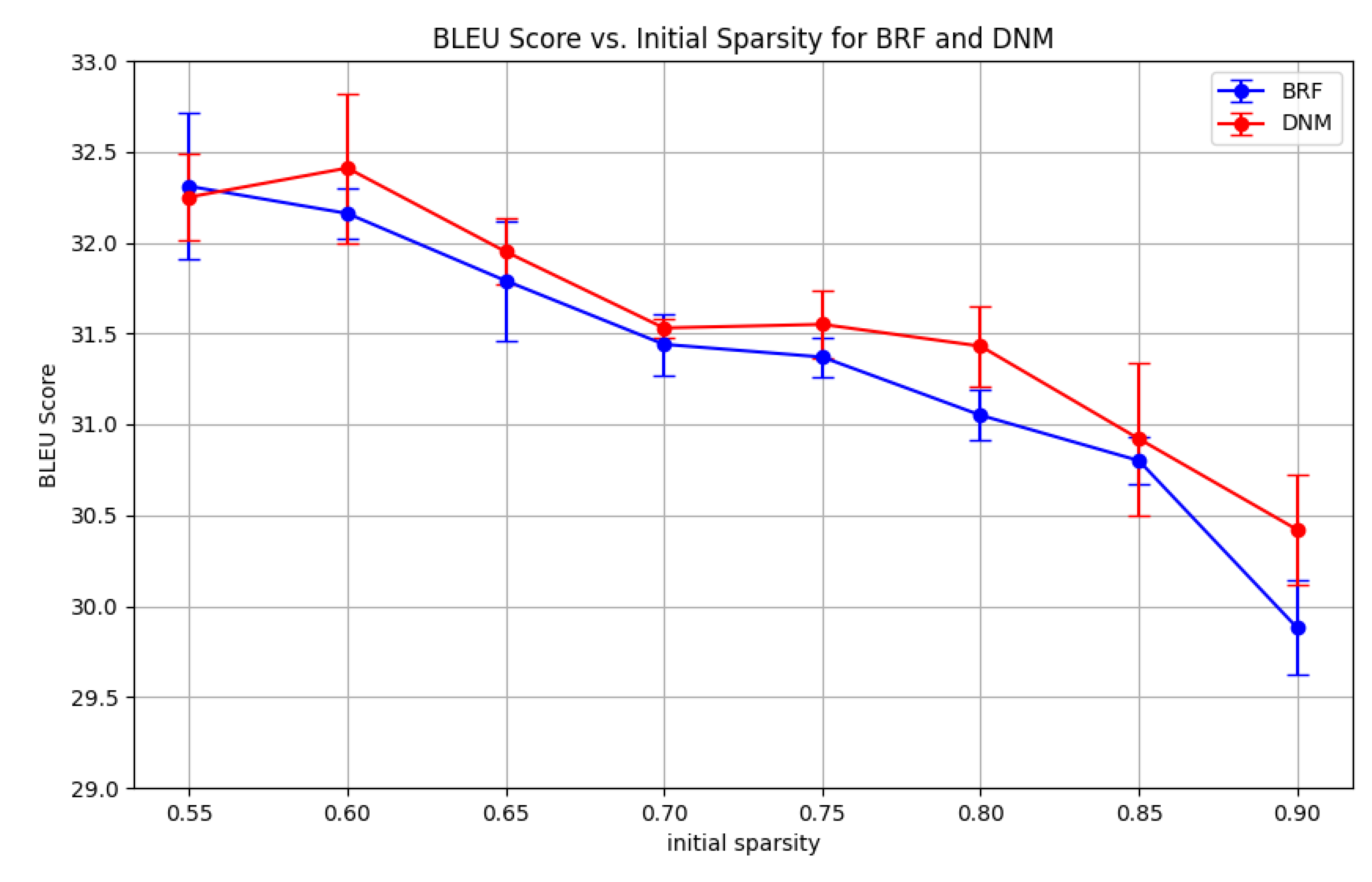
As demonstrated in Subsection 4.3, DNM’s impact on CHTss is similar to the BRF baseline. This is expected, since CHTss’s gradual decay mechanism starts from a dense 50% state, where the initial network structure is less critical and the topological advantages of DNM are less pronounced. To prove that at higher sparsities DNM can largely outperform BRF, we tested both models on the Multi30k translation task at 95% final sparsity and various initial sparsity levels (Table A3, Figure A5). As expected, when starting from a sparser state, DNM outperforms BRF by a larger margin. This suggests that DNM is particularly effective when the initial network structure plays a more significant role in determining performance, as is the case at higher sparsity levels. To further validate this, we fixed DNM’s parametric configuration across initial sparsity levels, using the best performing parametric configuration found from the experiment conducted in Subsection 4.3. The results (Table A4, Figure A6) confirm that DNM consistently outperforms BRF across all tested initial sparsity levels, with the performance gap widening as the initial sparsity increases. This reinforces the conclusion that DNM’s structured approach to sparse connectivity is particularly advantageous in scenarios where the initial network topology is crucial for learning efficacy.
Table A3.
Comparison of DNM and BRF initializations on CHTss for machine translation on the Multi-30k en-de dataset at 95% final sparsity. The results for both DNM and BRF correspond to those of the best performing parametric configurations of the models for each initial sparsity. The initial sparsity level is varied, taking values 0.50, 0.60, 0.75, 0.90. The entries represent the BLEU scores, averaged over 3 seeds ± the standard error.
| With parameter search | ||||
|---|---|---|---|---|
| 0.50 | 0.60 | 0.75 | 0.90 | |
| DNM | 32.71±0.35 | 32.71±0.43 | 32.28±0.29 | 31.45±0.35 |
| BRF | 32.86±0.16 | 32.16±0.14 | 31.20±0.36 | 29.81±0.37 |
Figure A5.
CHTss with varying initial sparsity and fixed DNM parameters. The figure compares the performance of DNM and BRF initializations for CHTss over various initial sparsity levels for machine translation tasks on Multi-30k at 90% final sparsity. The results for both DNM and BRF correspond to those of the best performing parametric configurations of the models for each initial sparsity. The entries represent the BLEU scores, averaged over 3 seeds.
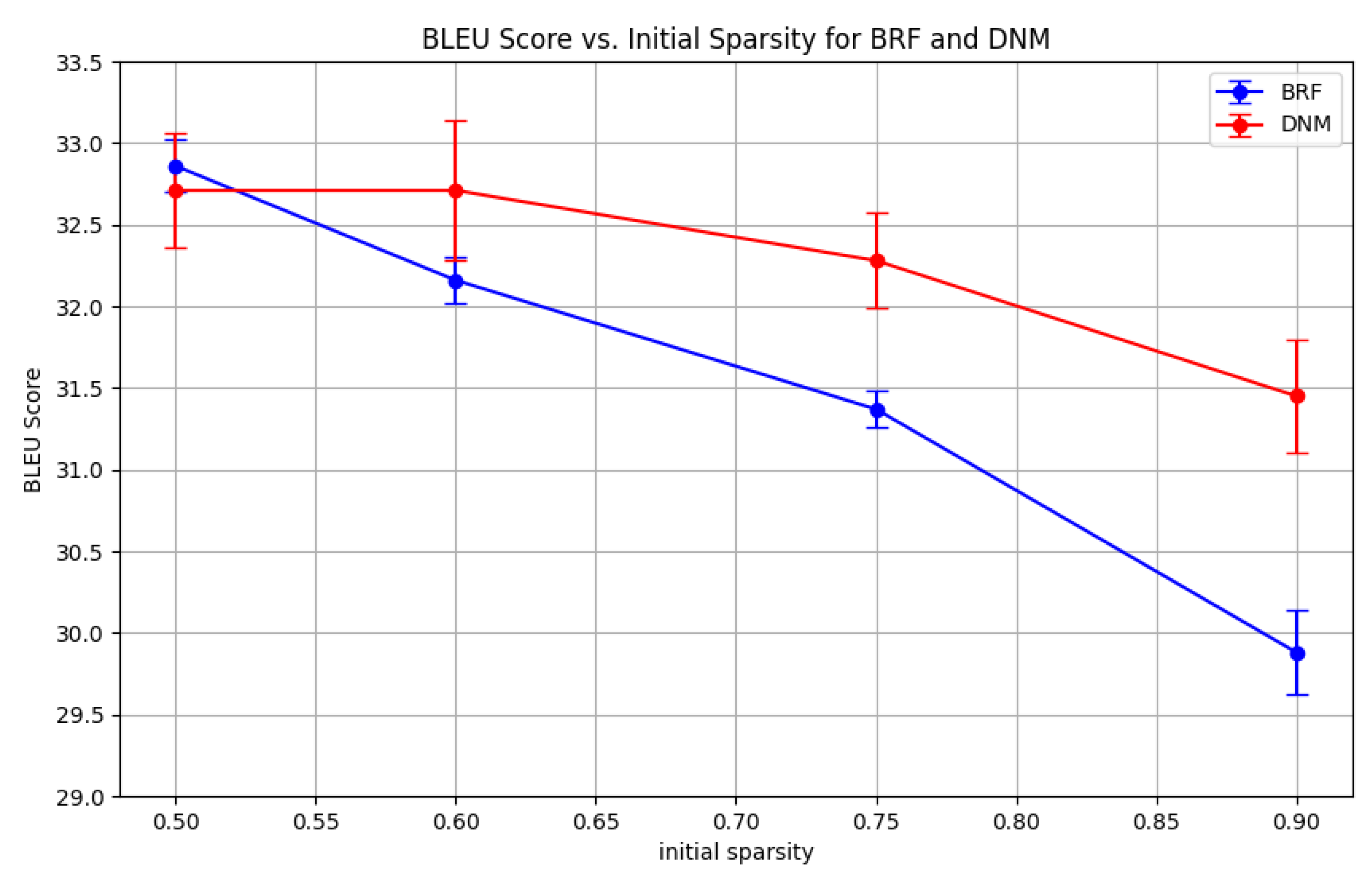
Table A4.
Comparison of DNM and BRF initializations on CHTss for machine translation on the Multi-30k en-de dataset at 95% final sparsity. DNM’s parametric configuration is fixed across initial sparsity levels, using the best performing parametric configuration found from the experiment performed in Subsection 4.3. BRF’s performances are chosen taking the best performing parametric configurations. The initial sparsity level is varied at steps of 0.05 between 0.55 and 0.90. The entries represent the BLEU scores, averaged over 3 seeds.
| No DNM parameter search | ||||||||
|---|---|---|---|---|---|---|---|---|
| 0.55 | 0.60 | 0.65 | 0.70 | 0.75 | 0.80 | 0.85 | 0.90 | |
| DNM | 32.25 | 32.41 | 31.95 | 31.53 | 31.55 | 31.43 | 30.92 | 30.42 |
| BRF | 32.31 | 32.16 | 31.79 | 31.44 | 31.37 | 31.05 | 30.80 | 29.88 |
Figure A6.
CHTss with varying initial sparsity. The figure compares the performance of DNM and BRF initializations for CHTss over various initial sparsity levels for machine translation tasks on Multi-30k at 90% final sparsity. DNM’s parametric configuration is fixed across initial sparsity levels, using the best performing parametric configuration found from the experiment performed in Subsection 4.3. BRF’s performances are chosen taking the best performing parametric configurations. The entries represent the BLEU scores, averaged over 3 seeds.
Appendix H. Analysis of the Bounded Layer Border Wiring Pattern
To investigate the impact of the layer border wiring pattern setting, we compare the default wrap-around topology with the bounded topology. We tested the bounded configuration on the same image classification tasks as the default, at 99% sparsity using static sparse training (Table A5), SET (Table A6), CHTs (Table A7), and CHTss (Table A8). Overall, the performance of the bounded model is comparable to that of the default wrap-around model, with some variations across datasets and training methods. The bounded model outperforms the default on Fashion MNIST and CIFAR10 when using static sparse training and SET, while the default has a slight edge on MNIST and EMNIST. For CHTs and CHTss, the results are mixed, with each model excelling in different datasets. These findings suggest that while strict locality can be beneficial in certain contexts, the flexibility of wrap-around connections may provide advantages in others. The choice of wiring pattern should thus be informed by the specific characteristics of the task and dataset at hand.
Table A5.
Comparison of wrap-around and bounded topology performances for static sparse training of MLPs. The entries represent the accuracy for image classification over different datasets at 99% sparsity, averaged over 3 seeds ± their standard error.
Table A5.
Comparison of wrap-around and bounded topology performances for static sparse training of MLPs. The entries represent the accuracy for image classification over different datasets at 99% sparsity, averaged over 3 seeds ± their standard error.
| Static Sparse Training | ||||
|---|---|---|---|---|
| MNIST | EMNIST | Fashion_MNIST | CIFAR10 | |
| Bounded | 97.64±0.10 | 84.00±0.06 | 89.19±0.01 | 61.63±0.18 |
| Wrap-around | 97.82±0.03 | 84.76±0.13 | 88.47±0.03 | 59.04±0.17 |
Table A6.
Comparison of wrap-around and bounded topology performances for SET initialization on MLPs. The entries represent the accuracy for image classification over different datasets at 99% sparsity, averaged over 3 seeds ± their standard error.
Table A6.
Comparison of wrap-around and bounded topology performances for SET initialization on MLPs. The entries represent the accuracy for image classification over different datasets at 99% sparsity, averaged over 3 seeds ± their standard error.
| SET | ||||
|---|---|---|---|---|
| MNIST | EMNIST | Fashion_MNIST | CIFAR10 | |
| Bounded | 98.40±0.02 | 86.52±0.02 | 89.78±0.09 | 65.67±0.18 |
| Wrap-around | 98.36±0.05 | 86.50±0.06 | 89.75±0.04 | 64.81±0.01 |
Table A7.
Comparison of wrap-around and bounded topology performances for CHTs initialization on MLPs. The entries represent the accuracy for image classification over different datasets at 99% sparsity, averaged over 3 seeds ± their standard error.
Table A7.
Comparison of wrap-around and bounded topology performances for CHTs initialization on MLPs. The entries represent the accuracy for image classification over different datasets at 99% sparsity, averaged over 3 seeds ± their standard error.
| CHTs | ||||
|---|---|---|---|---|
| MNIST | EMNIST | Fashion_MNIST | CIFAR10 | |
| Bounded | 98.66±0.03 | 87.35±0.00 | 90.68±0.09 | 68.03±0.14 |
| Wrap-around | 98.62±0.01 | 87.40±0.04 | 90.62±0.16 | 68.76±0.11 |
Table A8.
Comparison of wrap-around and bounded topology performances for CHTss initialization on MLPs. The entries represent the accuracy for image classification over different datasets at 99% sparsity, averaged over 3 seeds ± their standard error.
Table A8.
Comparison of wrap-around and bounded topology performances for CHTss initialization on MLPs. The entries represent the accuracy for image classification over different datasets at 99% sparsity, averaged over 3 seeds ± their standard error.
| CHTss | ||||
|---|---|---|---|---|
| MNIST | EMNIST | Fashion_MNIST | CIFAR10 | |
| Bounded | 98.66±0.03 | 87.37±0.04 | 90.68±0.09 | 68.03±0.14 |
| Wrap-around | 98.90±0.01 | 87.55±0.01 | 90.88±0.03 | 68.50±0.21 |
Appendix I. Transferability of Optimal Topologies
A critical question for our generative model of network topology is whether its principles are generalizable across different tasks. To investigate this, we conducted a transfer learning experiment to assess if an optimal topology discovered on a simpler task could be effectively applied to more complex ones. This tests the hypothesis that the DNM can capture fundamental structural priors beneficial for a class of problems, such as image classification, thereby reducing the need for extensive hyperparameter searches on every new dataset.
Experimental Design
We identified the best-performing DNM hyperparameter configuration from the static sparse training experiments on the MNIST dataset, as analyzed in Section 5. This configuration, which generates a scale-free, hierarchical network, was then used directly to initialize MLP models for the more challenging EMNIST, Fashion MNIST, and CIFAR-10 datasets. We then compared its performance against the other baseline initialization methods and against the DNM models whose hyperparameters were specifically tuned for each target task ("DNM (Task-Specific Best)").
Results
The results, summarized in Table A9, demonstrate the remarkable effectiveness of the transferred topology. On EMNIST and CIFAR10, the DNM (Transferred) model significantly outperforms the random, BSW, BRF, and Ramanujan initializations. On Fashion MNIST, however, BSW slightly outperforms it. Its performance is only marginally lower than that of the task-specific DNM.
Table A9.
Performance of the transferred DNM topology on static sparse training at 99% sparsity. The "DNM (Transferred)" model uses the single best hyperparameter configuration found on MNIST for all three target tasks. Its performance is compared to baselines and to the best task-specific DNM configuration. Scores are the accuracy averaged over 3 seeds ± standard error. Bold values denote the best performance.
| Static Sparse Training | |||
|---|---|---|---|
| Fashion MNIST | EMNIST | CIFAR10 | |
| FC | 90.88±0.02 | 87.13±0.04 | 62.85±0.16 |
| CSTI | 88.52±0.14 | 84.66±0.13 | 52.64±0.30 |
| SNIP | 87.85±0.22 | 84.08±0.08 | 61.81±0.58 |
| Random | 87.34±0.11 | 82.66±0.08 | 55.28±0.09 |
| BSW | 88.18±0.18 | 82.94±0.06 | 56.54±0.15 |
| BRF | 87.41±0.13 | 82.98±0.02 | 54.73±0.07 |
| Ramanujan | 86.45±0.15 | 81.80±0.13 | 55.05±0.40 |
| DNM (Fine-tuned) | 89.19±0.01 | 84.76±0.13 | 61.63±0.18 |
| DNM (Transferred) | 87.98±0.06 | 83.67±0.06 | 58.70±0.42 |
Discussion
This experiment strongly suggests that the structural principles identified by DNM as optimal for MNIST serve as a powerful and generalizable prior for other image classification tasks. The ability to transfer a high-performing topology with minimal performance loss has significant practical implications, as it can drastically reduce the computational cost associated with architecture search for new applications. This finding reinforces the idea that bio-inspired, structured initialization is not merely a task-specific trick but a robust strategy for building efficient sparse networks.
Appendix J. Reproduction statement
All experiments were conducted on NVIDIA A100 80GB GPUs. MLP and Transformer models were trained using a single GPU. The code to reproduce the experiments will be made publicly available upon publication.
Appendix K. Claim of LLM Usage
The authors declare that Large Language Models (LLMs) were used in the writing process of this manuscript. However, the core idea and principles of the article are entirely original and were not generated by LLMs.
References
- Drachman, D.A. Do we have brain to spare?, 2005.
- Walsh, C.A. Peter Huttenlocher (1931–2013). Nature 2013, 502, 172–172.
- Cuntz, H.; Forstner, F.; Borst, A.; Häusser, M. One rule to grow them all: a general theory of neuronal branching and its practical application. PLoS computational biology 2010, 6, e1000877. [CrossRef]
- London, M.; Häusser, M. Dendritic computation. Annu. Rev. Neurosci. 2005, 28, 503–532. [CrossRef]
- Larkum, M. A cellular mechanism for cortical associations: an organizing principle for the cerebral cortex. Trends in neurosciences 2013, 36, 141–151. [CrossRef]
- Poirazi, P.; Brannon, T.; Mel, B.W. Pyramidal neuron as two-layer neural network. Neuron 2003, 37, 989–999. [CrossRef]
- Lauditi, C.; Malatesta, E.M.; Pittorino, F.; Baldassi, C.; Brunel, N.; Zecchina, R. Impact of Dendritic Nonlinearities on the Computational Capabilities of Neurons. PRX Life 2025, 3, 033003.
- Baek, E.; Song, S.; Baek, C.K.; Rong, Z.; Shi, L.; Cannistraci, C.V. Neuromorphic dendritic network computation with silent synapses for visual motion perception. Nature Electronics 2024, 7, 454–465. [CrossRef]
- Jones, I.S.; Kording, K.P. Might a single neuron solve interesting machine learning problems through successive computations on its dendritic tree? Neural Computation 2021, 33, 1554–1571. [CrossRef]
- Jones, I.S.; Kording, K.P. Do biological constraints impair dendritic computation? Neuroscience 2022, 489, 262–274. [CrossRef]
- LeCun, Y.; Bottou, L.; Bengio, Y.; Haffner, P. Gradient-based learning applied to document recognition. Proceedings of the IEEE 2002, 86, 2278–2324. [CrossRef]
- Cohen, G.; Afshar, S.; Tapson, J.; Van Schaik, A. EMNIST: Extending MNIST to handwritten letters. In Proceedings of the 2017 international joint conference on neural networks (IJCNN). IEEE, 2017, pp. 2921–2926.
- Xiao, H.; Rasul, K.; Vollgraf, R. Fashion-mnist: a novel image dataset for benchmarking machine learning algorithms. arXiv preprint arXiv:1708.07747 2017.
- Krizhevsky, A. Learning Multiple Layers of Features from Tiny Images 2009. pp. 32–33.
- Vaswani, A.; Shazeer, N.; Parmar, N.; Uszkoreit, J.; Jones, L.; Gomez, A.N.; Kaiser, .; Polosukhin, I. Attention is all you need. Advances in neural information processing systems 2017, 30.
- Elliott, D.; Frank, S.; Sima’an, K.; Specia, L. Multi30K: Multilingual English-German Image Descriptions. In Proceedings of the Proceedings of the 5th Workshop on Vision and Language. Association for Computational Linguistics, 2016, pp. 70–74. https://doi.org/10.18653/v1/W16-3210.
- Cettolo, M.; Niehues, J.; Stüker, S.; Bentivogli, L.; Federico, M. Report on the 11th IWSLT evaluation campaign. In Proceedings of the Proceedings of the 11th International Workshop on Spoken Language Translation: Evaluation Campaign; Federico, M.; Stüker, S.; Yvon, F., Eds., Lake Tahoe, California, 4-5 2014; pp. 2–17.
- Bojar, O.; Chatterjee, R.; Federmann, C.; Graham, Y.; Haddow, B.; Huang, S.; Huck, M.; Koehn, P.; Liu, Q.; Logacheva, V.; et al. Findings of the 2017 conference on machine translation (wmt17). Association for Computational Linguistics, 2017.
- Erdős, P.; Rényi, A. On the evolution of random graphs. Publication of the Mathematical Institute of the Hungarian Academy of Sciences 1960, 5, 17–60.
- Watts, D.J.; Strogatz, S.H. Collective dynamics of ’small-world’ networks. Nature 1998, 393, 440–442. [CrossRef]
- Barabási, A.L.; Albert, R. Emergence of scaling in random networks. science 1999, 286, 509–512. [CrossRef]
- Zhang, Y.; Zhao, J.; Wu, W.; Muscoloni, A.; Cannistraci, C.V. Epitopological learning and Cannistraci-Hebb network shape intelligence brain-inspired theory for ultra-sparse advantage in deep learning. In Proceedings of the The Twelfth International Conference on Learning Representations, 2024.
- Zhang, Y.; Zhao, J.; Wu, W.; Muscoloni, A. Epitopological learning and cannistraci-hebb network shape intelligence brain-inspired theory for ultra-sparse advantage in deep learning. In Proceedings of the The Twelfth International Conference on Learning Representations, 2024.
- Lee, N.; Ajanthan, T.; Torr, P.H. Snip: Single-shot network pruning based on connection sensitivity. arXiv preprint arXiv:1810.02340 2018.
- Kalra, S.A.; Biswas, A.; Mitra, P.; Basu, B. Sparse Neural Architectures via Deterministic Ramanujan Graphs. Transactions on Machine Learning Research.
- Zhang, Y.; Cerretti, D.; Zhao, J.; Wu, W.; Liao, Z.; Michieli, U.; Cannistraci, C.V. Brain network science modelling of sparse neural networks enables Transformers and LLMs to perform as fully connected. arXiv preprint arXiv:2501.19107 2025.
- Cacciola, A.; Muscoloni, A.; Narula, V.; Calamuneri, A.; Nigro, S.; Mayer, E.A.; Labus, J.S.; Anastasi, G.; Quattrone, A.; Quartarone, A.; et al. Coalescent embedding in the hyperbolic space unsupervisedly discloses the hidden geometry of the brain. arXiv preprint arXiv:1705.04192 2017.
- Mocanu, D.C.; Mocanu, E.; Stone, P.; Nguyen, P.H.; Gibescu, M.; Liotta, A. Scalable training of artificial neural networks with adaptive sparse connectivity inspired by network science. Nature communications 2018, 9, 2383. [CrossRef]
- Evci, U.; Gale, T.; Menick, J.; Castro, P.S.; Elsen, E. Rigging the lottery: Making all tickets winners. In Proceedings of the International conference on machine learning. PMLR, 2020, pp. 2943–2952.
- Cettolo, M.; Girardi, C.; Federico, M. Wit3: Web inventory of transcribed and translated talks. Proceedings of EAMT 2012, pp. 261–268.
- Lü, L.; Pan, L.; Zhou, T.; Zhang, Y.C.; Stanley, H.E. Toward link predictability of complex networks. Proceedings of the National Academy of Sciences 2015, 112, 2325–2330. [CrossRef]
- Newman, M.E. Modularity and community structure in networks. Proceedings of the national academy of sciences 2006, 103, 8577–8582.
- Cannistraci, C.V.; Muscoloni, A. Geometrical congruence, greedy navigability and myopic transfer in complex networks and brain connectomes. Nature Communications 2022, 13, 7308. [CrossRef]
- Muscoloni, A.; Thomas, J.M.; Ciucci, S.; Bianconi, G.; Cannistraci, C.V. Machine learning meets complex networks via coalescent embedding in the hyperbolic space. Nature communications 2017, 8, 1615. [CrossRef]
- Balasubramanian, M.; Schwartz, E.L. The isomap algorithm and topological stability. Science 2002, 295, 7–7. [CrossRef]
- Muscoloni, A.; Abdelhamid, I.; Cannistraci, C.V. Local-community network automata modelling based on length-three-paths for prediction of complex network structures in protein interactomes, food webs and more. BioRxiv 2018, p. 346916.
- Kingma, D.P.; Ba, J. Adam: A method for stochastic optimization. arXiv preprint arXiv:1412.6980 2014.
- Bellec, G.; Kappel, D.; Maass, W.; Legenstein, R. Deep rewiring: Training very sparse deep networks. arXiv preprint arXiv:1711.05136 2017.
- Yuan, G.; Ma, X.; Niu, W.; Li, Z.; Kong, Z.; Liu, N.; Gong, Y.; Zhan, Z.; He, C.; Jin, Q.; et al. Mest: Accurate and fast memory-economic sparse training framework on the edge. Advances in Neural Information Processing Systems 2021, 34, 20838–20850.
- Jayakumar, S.; Pascanu, R.; Rae, J.; Osindero, S.; Elsen, E. Top-kast: Top-k always sparse training. Advances in Neural Information Processing Systems 2020, 33, 20744–20754.
- Lasby, M.; Golubeva, A.; Evci, U.; Nica, M.; Ioannou, Y. Dynamic sparse training with structured sparsity. arXiv preprint arXiv:2305.02299 2023.
- Lubotzky, A.; Phillips, R.; Sarnak, P. Ramanujan graphs. Combinatorica 1988, 8, 261–277.
- Marcus, A.; Spielman, D.A.; Srivastava, N. Interlacing families I: Bipartite Ramanujan graphs of all degrees. In Proceedings of the 2013 IEEE 54th Annual Symposium on Foundations of computer science. IEEE, 2013, pp. 529–537.
- Muscoloni, A.; Michieli, U.; Zhang, Y.; Cannistraci, C.V. Adaptive network automata modelling of complex networks 2022.
| 1 | To facilitate an intuitive exploration of this landscape, we have developed an interactive web application where readers can adjust the model’s parameters and visualize the resulting network structures. The application is available at: https://dendritic-network-model.streamlit.app/
|
Figure 1.
The Dendritic Network Model. Traditional models (top) treat neurons as simple integrators, ignoring the structure of synaptic inputs. In contrast, our brain-inspired approach (bottom) organizes connections into dendritic branches, creating a structured topology where distinct groups of inputs are processed locally.
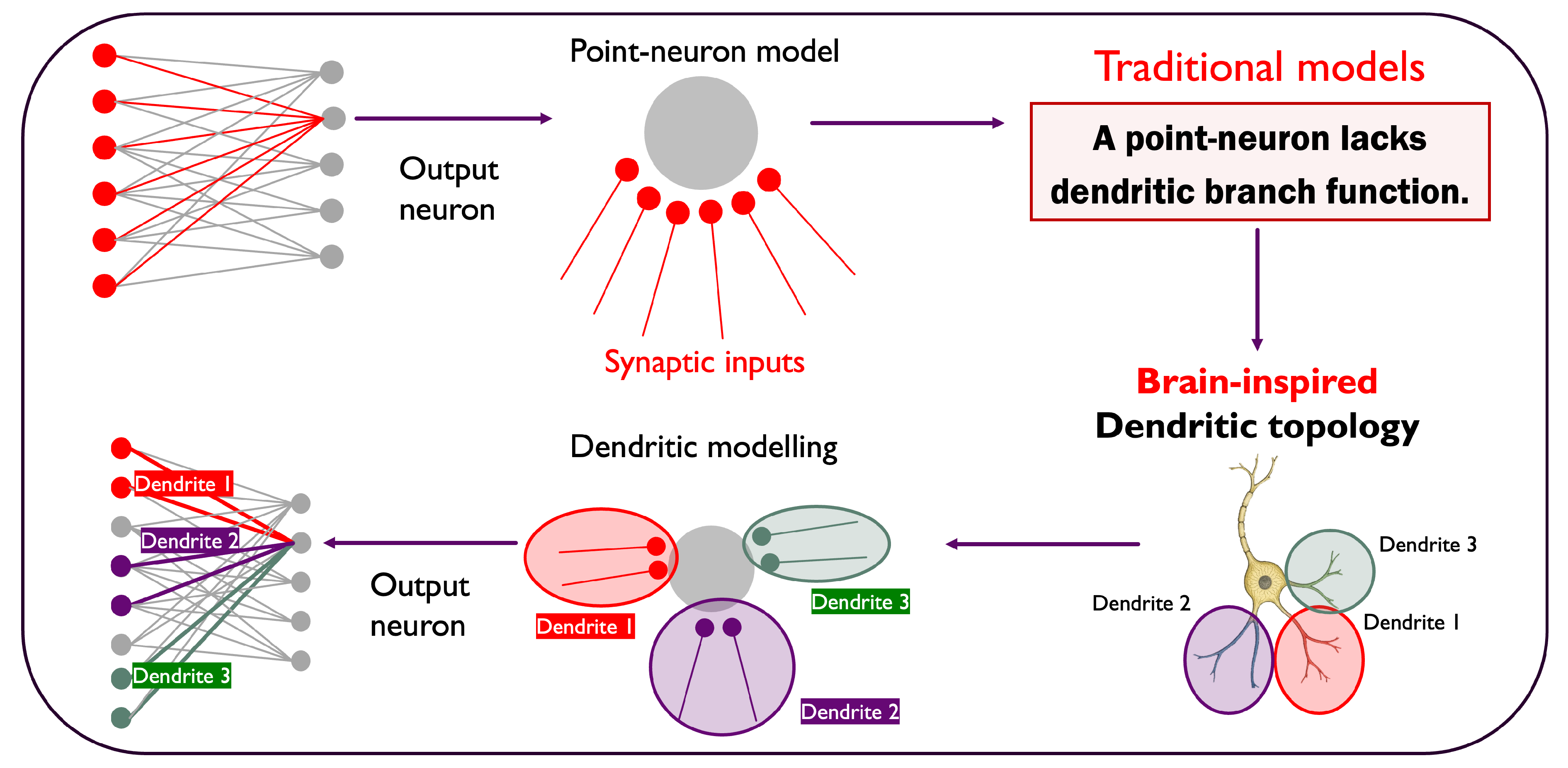
Figure 2.
Geometric and topological characterization of the Dendritic Network Model. The figure compares a baseline random network (a) with various DNM configurations (b-d) for a 3-layered MLP of size with 90% sparsity. Each panel shows a coalescent embedding in hyperbolic space (left), the first layer’s adjacency matrix (top right), a bipartite graph representation (bottom right), and key network science metrics: characteristic path length L, modularity (Q), structural consistency (), and the power law exponent of the degree distribution (). The network in (b) is a standard DNM model, generated using fixed distributions for all parameters, , and . Panels (c-d) modify this standard configuration by switching a single parameter’s distribution to spatial Gaussian: (c) degree distribution, (d) synaptic distribution.
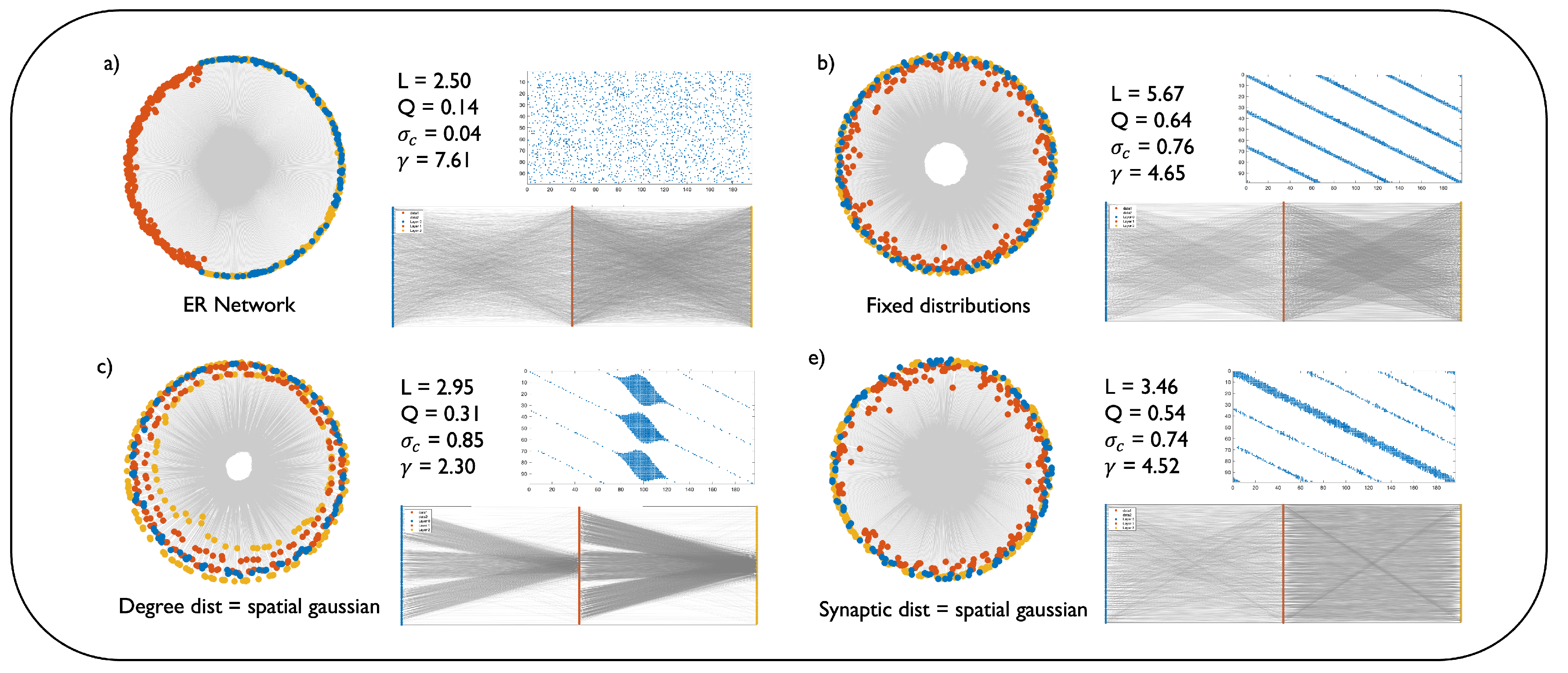
Figure 3.
Representation of the best performing DNM models on image classification. The figure compares the best performing DNM architectures on MNIST and Fashion MNIST (a), EMNIST (b), and CIFAR10 (c). Each panel shows the network’s adjacency matrix (top) and the network’s layerwise representation (bottom). Furthermore, each panel exhibits the network’s topological measures: characteristic path length L, modularity (Q), structural consistency (), and the power law exponent of the degree distribution ().
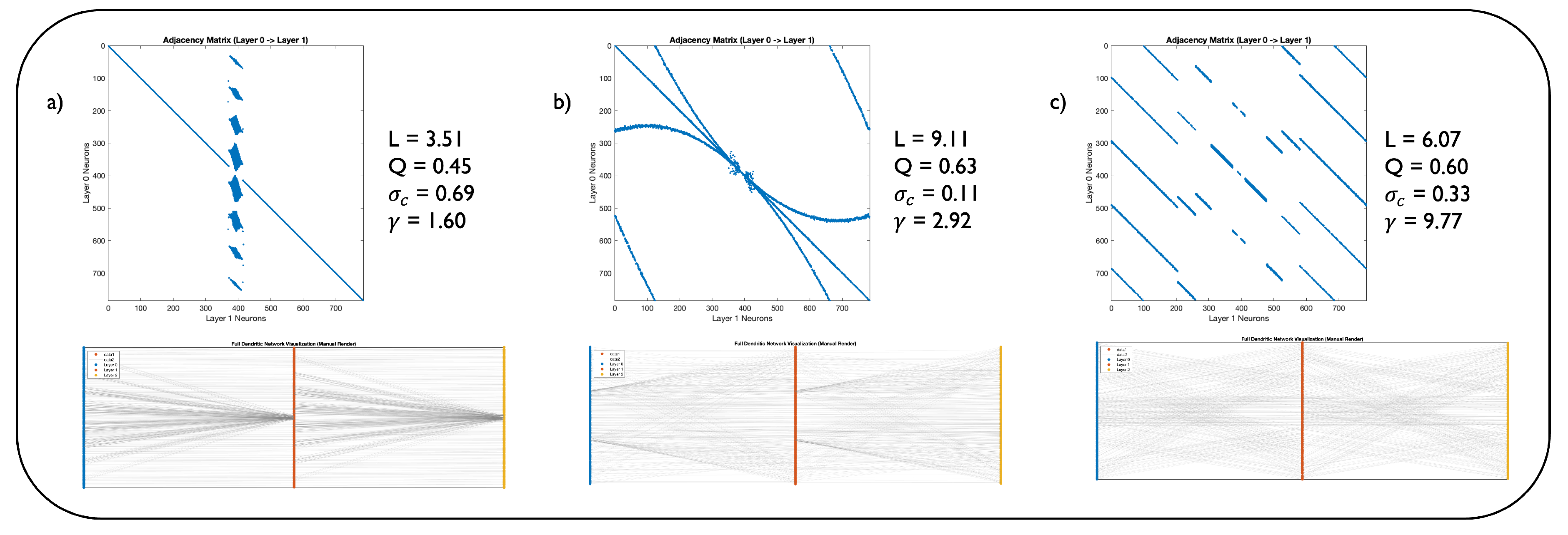
Table 1.
Image classification accuracy of statically trained, 99% sparse MLPs with different initial network topologies, compared to the fully-connected (FC) model. The scores are averaged over 3 seeds ± their standard errors. Bold values denote the best performance amongst initialization methods different from CSTI and SNIP.
| Static Sparse Training | ||||
|---|---|---|---|---|
| MNIST | Fashion MNIST | EMNIST | CIFAR10 | |
| FC | 98.78±0.02 | 90.88±0.02 | 87.13±0.04 | 62.85±0.16 |
| CSTI | 98.07±0.02 | 88.52±0.14 | 84.66±0.13 | 52.64±0.30 |
| SNIP | 97.59±0.08 | 87.85±0.22 | 84.08±0.08 | 61.81±0.58 |
| Random | 96.72±0.04 | 87.34±0.11 | 82.66±0.08 | 55.28±0.09 |
| BSW | 97.32±0.02 | 88.18±0.18 | 82.94±0.06 | 56.54±0.15 |
| BRF | 96.85±0.01 | 87.41±0.13 | 82.98±0.02 | 54.73±0.07 |
| Ramanujan | 96.51±0.17 | 86.45±0.15 | 81.80±0.13 | 55.05±0.40 |
| DNM | 97.82±0.03 | 89.19±0.01 | 84.76±0.13 | 61.63±0.18 |
Table 2.
Image classification on MNIST, Fashion MNIST, EMNIST, and CIFAR-10 of the SET model on MLPs with 99% sparsity over various topological initialization methods, compared to the fully-connected (FC) model. The scores indicate the accuracy of the models, averaged over 3 seeds ± their standard errors. Bold values denote the best performance amongst initialization methods different from CSTI and SNIP. Sparse models that surpass the fully connected network are marked with "*".
| SET | ||||
|---|---|---|---|---|
| MNIST | Fashion MNIST | EMNIST | CIFAR10 | |
| FC | 98.78±0.02 | 90.88±0.02 | 87.13±0.04 | 62.85±0.16 |
| SNIP | 98.31±0.05 | 89.49±0.05 | 86.44±0.09 | 64.26±0.14 |
| CSTI | 98.47±0.02 | 89.91±0.11 | 86.66±0.06 | 65.05±0.14 |
| Random | 98.14±0.02 | 89.00±0.09 | 86.31±0.08 | 62.70±0.11 |
| BSW | 98.25±0.02 | 89.25±0.03 | 86.26±0.08 | 63.66±0.07* |
| BRF | 98.25±0.01 | 89.44±0.01 | 86.20±0.04 | 62.64±0.10 |
| Ramanujan | 97.96±0.05 | 89.16±0.07 | 85.80±0.03 | 62.58±0.20 |
| DNM | 98.40±0.02 | 89.78±0.09 | 86.52±0.02 | 65.67±0.18* |
Table 3.
Image classification on MNIST, Fashion MNIST, EMNIST, and CIFAR-10 of the RigL model on MLPs with 99% sparsity over various topological initialization methods, compared to the fully-connected (FC) model. The scores indicate the accuracy of the models, averaged over 3 seeds ± their standard errors. Bold values denote the best performance amongst initialization methods different from CSTI and SNIP. Sparse models that surpass the fully connected network are marked with "*".
| RigL | ||||
|---|---|---|---|---|
| MNIST | Fashion MNIST | EMNIST | CIFAR10 | |
| FC | 98.78±0.02 | 90.88±0.02 | 87.13±0.04 | 62.85±0.16 |
| SNIP | 98.75±0.04 | 89.89±0.01 | 87.34±0.03 | 63.79±0.23 |
| CSTI | 98.76±0.02 | 90.14±0.10 | 87.41±0.01 | 60.52±0.31 |
| Random | 98.61±0.01 | 89.53±0.04 | 86.99±0.09 | 64.24±0.07* |
| BSW | 98.71±0.06 | 89.85±0.07 | 87.18±0.07* | 65.06±0.19* |
| BRF | 98.65±0.03 | 89.76±0.09 | 87.08±0.05 | 64.33±0.16* |
| Ramanujan | 98.42±0.03 | 89.80±0.07 | 87.09±0.04 | 64.31±0.08* |
| DNM | 98.75±0.04 | 90.08±0.09 | 87.28±0.28* | 65.68±0.01* |
Table 4.
Image classification on CIFAR-10 of the CHTs and CHTss models on MLPs with 99% sparsity, compared to the fully-connected (FC) model. The scores indicate the accuracy of the models, averaged over 3 seeds ± their standard errors. Bold values denote the best performance amongst initialization methods different from CSTI.
| CSTI | Random | BSW | BRF | Ramanujan | DNM | |
|---|---|---|---|---|---|---|
| FC | 62.85±0.16 | |||||
| CHTs | 69.77±0.06 | 66.96±0.24 | 66.96±0.24 | 64.96±0.17 | 67.19±0.17 | 68.76±0.11 |
| CHTss | 71.29±0.14 | 66.89±0.23 | 66.89±0.23 | 64.96±0.17 | 67.37±0.12 | 68.50±0.21 |
Table 5.
Image classification on MNIST, Fashion MNIST, and EMNIST of the CHTs and CHTss models on MLPs with 99% sparsity over various topological initialization methods, compared to the fully-connected (FC) model. The scores indicate the accuracy of the models, averaged over 3 seeds ± their standard errors. Bold values denote the best performance amongst initialization methods different from CSTI. The performances that surpass CSTI are marked with "*".
| MNIST | Fashion MNIST | EMNIST | ||||
|---|---|---|---|---|---|---|
| CHTs | CHTss | CHTs | CHTss | CHTs | CHTss | |
| FC | 98.78±0.02 | 90.88±0.02 | 87.13±0.04 | |||
| CSTI | 98.81±0.04 | 98.83±0.02 | 90.93±0.03 | 90.81±0.11 | 87.82±0.04 | 87.52±0.04 |
| Random | 98.57±0.04 | 98.61±0.03 | 90.42±0.03 | 90.30±0.10 | 87.12±0.13 | 87.20±0.09 |
| BSW | 98.57±0.04 | 98.61±0.04 | 90.46±0.06 | 90.46±0.06 | 87.12±0.13 | 87.20±0.09 |
| BRF | 98.47±0.03 | 98.47±0.03 | 90.04±0.12 | 90.04±0.12 | 87.03±0.07 | 87.03±0.07 |
| Ramnujan | 98.57±0.03 | 98.57±0.03 | 89.82±0.14 | 98.78±0.08 | 87.24±0.08 | 87.24±0.08 |
| DNM | 98.66±0.03 | 98.90±0.01* | 90.68±0.09 | 90.88±0.03* | 87.40±0.04 | 87.55±0.01* |
Table 6.
Performance comparison on Multi30k en-de and IWSLT en-de translation tasks with varying sparsity levels (95% and 90%). BLEU scores (higher is better) are averaged over 3 seeds ± standard error. Bold indicates best performance for given sparsity and initialization; * denotes scores surpassing the fully connected model.
| Multi30k | IWSLT | |||
| 0.95 | 0.90 | 0.95 | 0.90 | |
| FC | 31.38±0.38 | 24.48±0.30 | ||
| CHTsB | 28.94±0.57 | 29.81±0.37 | 21.15±0.10 | 21.92±0.17 |
| CHTsD | 30.54±0.42 | 31.45±0.35* | 22.09±0.14 | 23.52±0.24 |
| CHTssB | 32.03±0.29* | 32.86±0.16* | 24.51±0.02* | 24.31±0.04 |
| CHTssD | 32.62±0.28* | 33.00±0.31* | 24.43±0.14 | 24.20±0.07 |
DDNM initialization. BBRF initialization.
Table 7.
Performance comparison on machine translation tasks across the WMT en-de dataset with varying final sparsity levels (95% and 90%). Contrary to the BRF model, the DNM model’s parameters were transferred from the best-performing combinations of previous tests, avoiding any parameter search. Entries are BLEU scores (higher is better), averaged over 3 seeds ± standard error. Bold values denote the best performance for a given sparsity and initialization.
| Model | WMT | |
| 0.95 | 0.90 | |
| FC | 25.52 | |
| CHTsB | 20.94±0.63 | 22.40±0.06 |
| CHTsD | 21.34±0.20 | 22.56±0.14 |
| CHTssB | 23.73±0.43 | 24.61±0.14 |
| CHTssD | 24.52±0.12 | 24.40±0.15 |
DDNM initialization. BBRF initialization.
Disclaimer/Publisher’s Note: The statements, opinions and data contained in all publications are solely those of the individual author(s) and contributor(s) and not of MDPI and/or the editor(s). MDPI and/or the editor(s) disclaim responsibility for any injury to people or property resulting from any ideas, methods, instructions or products referred to in the content. |
© 1996 by the authors. Licensee MDPI, Basel, Switzerland. This article is an open access article distributed under the terms and conditions of the Creative Commons Attribution (CC BY) license (https://creativecommons.org/licenses/by/4.0/).
Copyright: This open access article is published under a Creative Commons CC BY 4.0 license, which permit the free download, distribution, and reuse, provided that the author and preprint are cited in any reuse.


