Submitted:
14 April 2025
Posted:
15 April 2025
You are already at the latest version
Abstract
In this work, we explore the possibility of using the topology and weight distribution of the connectome of a Drosophila, or fruit fly, as a reservoir. Based on the information taken from the recently released full connectome, we create the connectivity matrix of an Echo State Network. Then, we implement two possible selection criteria to obtain a computationally convenient reservoir: the most connected neurons either preserving or not the relative proportion of different neuron classes, which are also included in the documented connectome. We then investigate the performance of such architectures and compare them to state-of-the-art reservoirs. The results show that the connectome-based architecture is significantly more resilient to overfitting compared to the standard implementation, particularly in cases already prone to overfitting. To further isolate the role of topology and synaptic weights, hybrid reservoirs with the connectome topology but randomized synaptic weights and the connectome weights but random topology are included in the study, demonstrating that both factors play a role in the increased overfitting resilience. Finally, we perform an experiment where the entire connectome is used as a reservoir. Despite the much higher number of trained parameters, the reservoir remains resilient to overfitting and has a lower normalized error (under 2%) at lower regularisation, compared to all other reservoirs trained with higher regularisation.
Keywords:
Reservoir Computing
; Biomimetics
; Drosophila
; Neural Networks
; Bio-inspired Computing
1. Introduction
In the ever-expanding field of machine learning (ML), increasing performance generally involves increasing model complexity, which in turn lengthens learning time [1,2,3]. This is typically achieved in one of two ways: either by adding more tunable parameters in neural networks (NN), such as Transformers, CNNs, or LSTMs [4,5,6,7], or by increasing the number of simulations in reinforcement learning and genetic algorithms [8,9,10].
However, some NN architectures, such as those used in reservoir computing, rely primarily on untrained synapses. Reservoir computing is a neural network paradigm that requires minimal training compared to most advanced ML models [11,12]. In a similar fashion to radial basis functions [13], reservoir computing relies on a nonlinear expansion of the dimensionality of the input data, which can then allow the problem to be solved linearly by a simple fully connected layer known as the readout. A noticeable difference between the two approaches is the recurrent nature of reservoirs, which adds a temporal buffering behavior to the system [14,15].
While the original concept of a reservoir consisted of virtually simulated pools of neurons that act as nonlinear expansions and temporal buffers for time series, physical implementations spanning several scientific fields have already been implemented, with examples including physical reservoir computing [16,17], photonic reservoir computing [18,19], and even memristor reservoir computing [20,21]. Broadly speaking, depending on the neuronal model used as the activation function [22,23], reservoir computing can be subdivided into liquid state machines (using spiking neurons), echo state networks (based on classical firing-rate neuron models), and time-delay reservoirs (introducing a temporal delay to the neuron dynamics).
The standard practice when creating a reservoir involves randomly initializing a desired number of neurons and synapses, adhering to specified sparsity, spectral radius, and distribution of non-zero weights [24,25]. While reservoir size, spectral radius, and sparsity significantly influence performance, other parameters often receive limited attention [26,27].
Despite these standardized practices, we still lack an understanding of what constitutes a good reservoir. Nature, on the other hand, has evolved neuronal systems over millions of years in the form of animal brains with a vast diversity of capacities, functions and specializations [28,29]. The example given by nature is often taken as an inspiration in the field, which in recent years has seen several attempts at bio-inspired and biologically plausible reservoir computing [30], from the imitation of neuronal plasticity [31] to the artificial implementation of the role of both neurons [32] and smaller biomolecules [33]. One study has taken a more drastic approach involving moving away from bio-inspiration and towards biomimicry by mapping the connectivity of connectomes of different species to a reservoir, in an attempt to investigate the performance of the former[34]. However, that study was limited both by the limited range of investigated hyperparameters and by the size of the investigated connectome, as at the time there was no reported case of a complete scan. In particular, whereas the reported result of connectome-based topology and randomized weights seems to imply a performance at best comparable to the standard fully randomized reservoir, the attempt at simulating also the synaptic weights was unsuccessful, further lowering performance for the heterogeneous connectivity case and completely failing for the homogeneous one. Following that study, connectome topologies have been proposed as an additional constraint on top of standard practice [35].
Nevertheless, thanks to the FlyWire project, the complete connectome of a fruit fly brain has been recently published [36]. This represents a huge milestone in neuroscience since it is the first complete scan of a relatively large brain. The only other documented complete scan of a connectome is of the Caenorhabditis elegans, with only 302 neurons [37], which has been investigated as an AI model [38] but contains too few neurons to be used for a thorough investigation with the field of reservoir computing. This recent scientific advancement provides a unique opportunity to analyze the topology and structure, as well as the role of synaptic weights, of an animal’s neural connectivity up to the scale of the entire connectome.
In this work, we explore the possibility of using the topology and synaptic connectivity of the scanned Drosophila connectome as a computational reservoir, comparing its performance to state-of-the-art implementations of reservoir computing. Whereas just the topology of limited parts of the Drosophila connectome, namely the olfactory system [39], has already yielded good preliminary results, to the authors’ knowledge, this is the first reported study that investigates and characterizes the combination of topology and synaptic weights for an entire connectome. To achieve this, we selected a notoriously chaotic and nonlinear time series: the 3-body problem [40]. Not only does it represent a historical milestone in the investigation of Lagrangian determinism, but it is also characterized by a greater challenge than other chaotic time series often used for benchmarking since the network is required to predict three time series simultaneously (the positions of the body). Moreover, it follows the recent interest in generative techniques for the n-body problem [41]. Our results demonstrate that the performance of the fly connectome is noticeably different from that of classical echo-state networks. Notably, reservoirs based on the fly connectome exhibit reduced overfitting in scenarios where overfitting plays a significant role [40].
2. Materials and Methods
2.1. Connectome Extraction
In order to represent the fly connectome as a reservoir, the data of both neurons and synapses are extracted using the CAVE client Python interface provided by the library caveclient. Neurons and neuronal classes are extracted simultaneously, saving the unique ID, the spatial position, and the cell class of every single neuron. For reference, Table 1 showcases all the different classes and their labels, and briefly describes their function. With the extracted information, it is possible to visualize the Drosophila connectome and to group its neurons according to their properties, as shown in Figure 1.
In order to create a reservoir, we retrieve all the synapses that have a given neuron as a pre-synaptic neuron, for every neuron previously collected. Queries of the database return the following information:
- the unique IDs of the pre-synaptic and post-synaptic neuron,
- the Cleft score: a measure of how well-defined the synaptic cleft is,
- the Connection score: a measure of the size of the synapse,
- the probability of the synaptic neurotransmitter being Gamma-Aminobutyric Acid, Acetylcholine, Glutamate, Octopamine, Serotonin, or Dopamine.
A first pre-processing of the data has been performed by applying a synapse quality filter: a simple threshold-based filtering of the synapses. First, synapses in which the post-synaptic neuron is not within the original set of classified neurons are deleted. Then, all synapses with either a Connection score or a Cleft score below a given threshold are also deleted, to avoid false positives. Following the guidelines of the original work [36], we have selected these thresholds to be 50 for the Cleft score and 100 for the Connection score. Whereas there are few synapses with a Connection score as high as , most of them are between and .
In order to transform the biological data into a connectivity matrix suitable for a reservoir, we have to determine the weights of the connections between neurons. Unfortunately, the provided database does not provide physiological, but only anatomical information. Since synaptic strength cannot be inferred from direct measurements, in this work we use the Connection score as an estimate of the strength of each synapse, assuming that larger synapses lead to stronger interactions, as shown for limited neuronal pools in literature [42,43].
Furthermore, information about the synaptic neurotransmitter is used in order to determine the signs of the weights in the connectivity matrix. Among all neurotransmitters, Gamma-aminobutyric acid is considered an inhibitory neurotransmitter, corresponding to a negative weight, and Acetylcholine and Glutamate are considered excitatory, corresponding to positive ones. Conversely, Octopamine, Serotonin, and Dopamine do not directly act as excitatory or inhibitory, but they rather modulate the resting potential of the post-synaptic neuron. Since ESNs feature a firing-rate neuronal model rather than a spiking one, they do not explicitly represent the resting potential, and thus the synapses that utilize modulatory neurotransmitters are not taken into consideration. For each synapse, we determine the neurotransmitter by taking the one with the highest probability in the database.
The result of this extraction process is a graph with 104909 nodes and the associated connectivity matrix. Computationally, a reservoir of such a size is too expensive to run (for comparison, most studies focus on ESNs with to neurons). To obtain a smaller reservoir, we have opted to retain a given number N of connected neurons, where N is arbitrary. To do that, we have implemented two possible selection criteria: ‘most connected’ and ‘proportional’. In the ‘most connected’ case, the N most connected neurons are selected. However, it is important for the fairness of comparison with the control classical reservoir that the selected subset of neurons consists of a single connected graph, in order to form a single reservoir of size N rather than two or more independent smaller ones. Therefore, only the largest connected component is considered, resulting in a reservoir of size . Then, the nearest neighbors are added to obtain the desired size, prioritizing the most connected neurons among all nearest neighbors.
In contrast, the ‘proportional’ criterion attempts to preserve the overall class distribution of the connectome, selecting the N most connected neurons while maintaining the same proportion of each class of neurons with respect to the entire connectome. Then, to obtain a single connected reservoir, the minimum number of nodes needed to connect all selected components is added. The resulting reservoir is of size . Finally, the least connected nodes are pruned from the graph, obtaining the desired reservoir size. Note that due to the requirement of a single connected subgraph, extra extraction steps have been added after the application of the selection criteria. These steps affect the final selected reservoir, which might differ significantly from the original N initially selected neurons.
To characterize the topology of each extracted reservoir, three standard metrics are taken into consideration: neuron degree, clustering coefficient, and shortest path length. The degree of a neuron i is the number of synapses incident to it, and the degree distribution captures the frequency of each across all neurons. The local clustering coefficient of a node i is defined as:
where is the number of edges between the neighbors of neruon i. The shortest path length is the minimum number of synapses traversed to reach neuron j from neuron i; we compute the distribution of all with across the entire reservoir.
2.2. Echo-State Network
The aim of this work is to investigate the Drosophila’s connectome as a reservoir within an ESN framework. Let us consider the equations governing an ESN (Figure 2):
where represents the reservoir state at time step n, is the reservoir weight matrix, is the input weight matrix, is the input signal, and is a scalar between 0 and 1, so that is the leakage rate.
The output readout layer is defined as:
where is the output weight matrix. The objective is to learn such that closely approximates a given target behavior (signal or label) . By organizing all target readouts into a matrix and all reservoir dynamics into a matrix , we obtain
which constitutes an overdetermined system in the unknown . The least squares solution, which minimizes the mean squared error (MSE), is given by:
A regularized solution, obtained via ridge regression [44], which minimizes the MSE along with a penalty on the weight magnitude, is given by:
where is the regularization parameter and is the identity matrix.
2.3. Time Series Generation
ESNs are often used for the classification and regression of time series. In particular, they have been shown to have good performance even when trained on chaotic time series [26]. In this study, ESNs are tested on the prediction of the circularly restricted 3-body problem (CR3BP). CR3BP trajectories have been obtained by propagating a set of initial conditions , where and are the initial positions and velocities, respectively. Those trajectories are then generated through propagation using the heyoka library [45] considering the mass ratio parameter of the earth-moon system and a timestep of of the normalized unit of time. Each resulting trajectory consists of 10000 datapoints and is subdivided into three subsets: washout, training, and test (Figure 3). The washout is used as an input to the reservoir with the sole purpose of nullifying the effect of the randomized initial state of the neurons. Then, the training set is fed to the reservoir to collect the data necessary for the aforementioned one-shot training, and the test set is used to evaluate the performance of the ESN.
2.4. Experimental Protocol
Figure 4 shows the experimental protocol that has been followed to obtain results. The extraction of the connectome, the filtering of the synapse, and the construction of the connectivity matrix are performed according to Section 2.1. According to previous literature [24], the parameter is set to , or the timestep, and the input scaling is fixed at . Note that the x, y, or z time series are presented to distinct subsets of the ESN neurons, which are selected at random before the training with equal probability. As a result, approximately a third of the ESN neurons receive one of the three Cartesian coordinates of the trajectory. In order to evaluate the Drosophila connectome as a reservoir, a comparative study is run with a traditional randomized reservoir through a Monte Carlo simulation. Both the connectome-based ESN and the classical implementation are constructed with the same sparsity, reservoir size N, input scaling, input matrix and initial output matrix prior to training. Specifically, each neuron in the ESN receives one of the three input time series, and all neurons are connected to the readout layer, thus . The parameters that are taken into consideration for the Monte Carlo simulation are the reservoir size N, the selection criteria used to construct the reservoir, the random distribution on the non-zero weights, the values, and the size of the forecast horizon. Note that the weights of the matrices of both reservoirs are scaled appropriately to ensure that they have the same spectral radius. Thus, the specific absolute weights are determined by this constraint and the imposed distribution. Every combination of tested hyperparameters is evaluated on five different trajectories, obtained by a variation of the initial conditions shown in Figure 3 and randomly re-initialized 10 times, resulting in 50 test cases per hyperparameter combination. In total, four different architectures are compared to each other: the control case, the connectome topology with randomized weights, the connectome topology with the connectome weights, and the connectome weights with a random topology. This allows us to isolate the contribution of the connectome topology from that of the synaptic weights. To evaluate the performance of the ESN, the normalized root mean squared error (nRMSE) is computed on both the training and the test set, as follows:
where is the squared Euclidean norm and is the mean of .
3. Results
3.1. Selection Criteria
First, it is important to investigate which subgraph of the entire connectome is taken into consideration, and how its characteristics, in terms of the nature of selected neurons and topology of the subgraph itself, are affected by the considered size N. As mentioned in Section 2.4, we have investigated two possible criteria: the most connected neurons, either regardless of the classes or proportional to the total class distribution shown in Figure 1. Figure 5 shows the general results regarding the sparsity and the non-zero weight distribution for the selection criteria as a function of N.
Starting from the sparsity at , we can observe that the subgraph selected with the ‘most connected’ criterion has a much lower sparsity than the ‘proportional’ criterion, as expected (see Figure 5 (A)). Moreover, the ‘most connected’ criterion leads to monotonically increasing sparsity, which is also likely. However, the sparsity of the ‘proportional’ criterion quickly drops as soon as and remains lower than the ‘most connected’ as N increases, showcasing similar asymptotic trends but at lower values. Therefore, it is clear that as N increases, the N most connected neurons do not form the most connected subgraph.
Concerning the distribution of extracted weights, Figure 5 (B) shows it as a function of N, whereas Figure 5 (C-D) show the probability density function (PDF) of the extracted weights in the case of ‘most connected’ and ‘proportional’ criteria, respectively. Noticeably, both criteria result in bimodal distributions, with steeper peaks as N increases, confirmed by the monotonically decreasing variance. According to recent comparisons for connectivity matrix extraction for connectomes [46], the extracted PDF highlights a significant amount of both positive and negative synapses, which is a fundamental requirement for achieving higher learning performance. Moreover, the presence of long tails in the distribution has been previously documented as a positive contribution to the reservoir’s performance [47]. However, note that in our results the two criteria differ in which peak is prevalent: the ‘most connected’ criterion is characterized by a higher presence of excitatory, or positive, synapses, whereas the ‘proportional’ criterion showcases a relatively higher number of inhibitory, or negative ones.
For a better insight into the selected networks, Figure 6 shows the scatterplots and the class distribution for a few of the selected reservoirs, namely both criteria and . Compared with the full connectome (see Figure 1), it is obvious that there are major differences. In the case of the ‘most connected’ criterion, is shown to include a very limited number of classes, with three overwhelmingly represented: ME, LO, and bilateral. This trend continues at , but the ME class eventually overcomes the others, representing close to half of the subgraph for . Moreover, as N increases, it is possible to observe a slightly larger number of different classes, but still far from the total number of classes.
Conversely, the proportion selection shows a much higher number of different classes already at . However, note that the distribution is not exactly proportional to the one shown in Figure 1 due to the constraint of imposed full connectivity (see Section 2.1). As N increases, it can be seen that first ME and later ME>LO start to be more and more represented. Although these two classes are the most represented in the entire connectome, they are still over-represented in the selected subgraph. This inevitably leads to the suppression of the other classes but still maintains a more diverse distribution than the ‘most connected’ criterion.
Finally, the two criteria largely differ in the locations of the selected neurons within the brain. As N increases, the ‘most connected’ criterion tends to produce a more symmetrical network, adding neurons almost equally from both hemispheres. In contrast, the ‘proportional’ criterion primarily selects neurons from a single hemisphere, with higher values of N corresponding to an ever more decentralized subgraph. This can be justified by the criterion trying to include all classes, even the ones that are absent in the more central cluster selected by the previous criterion, thus reaching the further layers. However, the limitation of a fixed N prevents the criterion from selecting a sufficient number of sensory neurons symmetrically, thus forcing it to primarily select from a single hemisphere.
As a last remark, the prevalence of ME and ME>LO neurons is hardly surprising. Firstly, the ME neurons represent the second processing stage of the optic lobe, which is known to process visual information, detect edges and motion, and be involved in contrast and color vision. Then, the ME>LO pathway relays information to the higher, more abstract visual areas, contributing to object recognition and image processing. These classes are not only the most abundant in the connectome of an animal that mainly deals with large quantities of visual inputs and processing, but they also represent the middle stages of this processing pipeline, being connected to both the sensory input neurons and the higher processing areas. Thus, these neurons are both the ‘most connected’ and the most over-represented when enforcing the connectedness of the constructed reservoir.
To have a deeper insight into the topology of the selected reservoir, Figure 7 shows the degree distribution, clustering coefficient distributions, and shortest path distribution, computed as described in Section 2.1. Moreover, it shows such metrics for both selection criteria and and , together with a random permutation of the selected reservoirs. Random permutations are obtained by taking the selected reservoir and randomly rearranging, or shuffling, the synapses. This allows us to investigate random topologies of the same sparsity and size of the selected networks.
The results clearly show that the extracted reservoirs have two topological characteristics that drastically differ from their randomized counterparts: the presence of a few highly connected neurons and more degrees of separation between any two given neurons. Shuffled topologies show a much more homogeneous configuration, with low clustering coefficients, a lower inter-neuron shortest path on average, and a Gaussian degree distribution. Whereas these properties are expected in a random graph [48], they are radically different from what we can observe in the case of the extracted topologies, both for and . Such topologies showcase a much higher clustering coefficient as shown in Figure 7 (C-D), possibly due to a few super-connected neurons (see Figure 7 (A-B)) and the presence of more separated areas, leading to the results of Figure 7 (E-F). It should also be noticed that such observations are valid for both reported sizes, indicating that the topological properties observed here seem to be intrinsic to any subset of the Drosophila connectome.
3.2. Single Simulation
As discussed in Section 2.2, the extracted reservoir is then included in an ESN, which is used for the prediction of multiple CR3BP trajectories. An important step in implementing an ESN is the washout, in which an initial set of points in the time series is used as input to the ESN in order to overwrite the initial random state of the neurons. Figure 8 (A-B) show the state of six random neurons during the washout in the case of the classical implementation and the connectome-extracted reservoir, respectively. It can be seen that neurons have a wide range of different behaviors, while the connectome-based architecture displays slightly reduced dynamics, never reaching the boundaries of the state.
To illustrate how these factors can impact the performance of the ESN, Figure 8 (C-J) shows the performance of the ESN as a predictor of a single CR3BP trajectory. Note that these results are specific for , , and a classical implementation obtained with a uniform distribution. Figure 8 (C-D) show that in the case of 1-timestep prediction, corresponding to 2.7 days, both architectures show good performance, ever so slightly in favor of the connectome-based reservoir. As expected, both architectures see a decrease in performance as the required prediction changes to 3, 7, and then 10 timesteps, which corresponds to 8.1, 18.9, and 27 days, respectively. However, the classical implementation shows a more rapid and more drastic deterioration of the performance, with significantly larger loops and greater errors, at least concerning the part of the trajectory around the larger body. However, this single case cannot justify a generalization to the remaining results.
As a more detailed illustration of the origin of the observed difference in performance, Figure 9 shows the same results as in Figure 8 but tested over five different trajectories, 10 trials per trajectory, and comparing the connectome-based reservoir both to a reservoir with non-zero weights sampled from either a uniform or Gaussian distribution, as described in Section 2.4. With this methodology, both architectures are re-initialized for each trial: in the case of the classic implementation, all architecture parameters are randomized, including topology, input connections, synaptic weights, and neuronal biases. Conversely, the connectome-based architecture maintains the same topology and synaptic weights, and only the input connections and biases are randomized. Note that the connectivity matrices of all cases are created with the same sparsity, which is imposed by the topology of the selected connectome subgraph, and they are rescaled to have the same spectral radius, which is restricted to be less than 1 in order to satisfy the echo state property, as indicated in the literature [24].
It is clear from the plots that the classic control reservoir tends to overfit the training, achieving a much lower nRMSE when tested on the training set. Conversely, the connectome-based reservoir shows a higher error on the training, but a consistently lower error on the test. However, both reservoirs show signs of overfitting. This can be explained by the fully connected readout, corresponding to , meaning that all of the reservoir’s neurons are connected to the ridge regression layers. This results in a large number of trainable parameters, which can cause overfitting, especially if paired with lower values of the regularization parameter .
3.3. Monte Carlo Simulations
To fully characterize the connectome-based reservoir both in terms of its topology and the distribution of non-zero weights, a comparative study has been performed according to Section 2.4. It is important to note, as previously discussed, that the hyperparameters involved in this investigation are the size of the selected reservoir N, the type of distribution used for the selection of random variables (either uniform or Gaussian), the prediction horizon, and the selection criterion used to extract the connectome-based reservoir from the full connectome. All other hyperparameters are kept constant across the tested cases, and every combination has been tested 10 times per trajectory over five different trajectories. The four different architectures which are part of the comparative study are:
- Random topology and random weight distribution, which is the standard way to create ESNs and it represents the control group.
- Connectome-based topology and extracted weight distribution, utilizing all the data extracted from the Drosophila connectome.
- Connectome-based topology and random weight distribution, to isolate solely the contribution of the topology of the connectome.
- Random topology and extracted weight distribution, to isolate solely the contribution of the weight distribution of the connectome.
Figure 10 and Figure 11 show the results of the Monte Carlo simulation for the ‘most connected’ and ‘proportional’ selection criteria, respectively.
Note that the results at confirm the insight given by the previous observations (see Figure 9), showing a decrease in performance of the classical implementation with respect to the other three. Moreover, it can be seen that such a difference increases as N increases. As expected, as the prediction horizon increases, there is a drop in performance (as shown in Figure 8). However, for all tested prediction horizons, the architecture with both connectome topology and connectome weights distribution does not show a decrease in performance for any tested N. In the case of the hybrid architectures, with connectome topology and random weights or vice-versa, the results show that their performance lies between that of the connectome-inspired architecture and the control one. This seems to indicate that both the non-zero weight distribution and the topology play an effective role in counteracting overfitting, given the improvement achieved just with the connectome topology or with its weight distribution. Moreover, the relative performance of the four tested cases is consistent across different conditions, with random topology and connectome-extracted weights always performing better than connectome topology and random weights, but worse than the fully biomimetic architecture, for large N. This result confirms that both the distribution of weights and the topology play a role in the increase in performance, but the effect of the distribution of weights is stronger.
Next, in the cases with lower regularization (i.e. ), it can be observed that the relative performance of all tested architectures is largely unchanged. Nevertheless, even the connectome topology and connectome weights case starts to show overfitting for larger N. Noticeably, this phenomenon appears earlier for short prediction horizons (Figure 10 (A-D) and Figure 11 (A-D)) than for longer horizons (Figure 10 (E-H) and Figure 11 (E-H)). This behavior can be explained by the lower regularization, which naturally makes the ESN more prone to overfitting. Moreover, these results indicate that ESNs with random Gaussian weight distribution are more resilient to overfitting compared to ones initialized with a uniform distribution, with smaller differences in performance between the four tested architectures as N increases. Similarly to the previous case, the distribution of weights taken from the connectome shows a stronger effect on the error reduction than the topology when considered in isolation, and the fully biomimetic architecture, despite starting to show a decrease in performance as N increases, is still the most resilient.
Conversely, the ESN behavior at shows drastically different trends. On one hand, there is no decrease in performance as N, and thus the number of trained degrees of freedom, increases. This result reinforces the conclusion that overfitting is the origin of the decrease in performance since higher values specifically counteract overfitting. On the other hand, the connectome topology and connectome weights architecture show the highest error almost consistently among different conditions. However, the connectome topology with random weight initialization still closely matches the performance of the classical implementation, and larger reservoirs with a uniform weight distribution eventually outperform the control architecture with random topology and random weights.
Comparing the corresponding subfigures in Figure 10 and Figure 11, the results are extremely similar, despite the differences in the topology of the selected connectome subgraphs that constitute the reservoirs (see Section 2.4). The most noticeable difference between the two Monte Carlo simulations is that the results corresponding to the architecture with connectome topology and random weights are closer to those for the control architecture in the case of ‘proportional’ selection. Moreover, this combination of topology and weight distribution is closer in performance to the control case than the architecture with connectome weights and random topology, which in turn is closer to the complete connectome-inspired architecture. This indicates that the contribution of the topology towards the mitigation of overfitting is present but small, and the observed bimodal distribution of non-zero weights (see Figure 6) plays a bigger role.
All investigated conditions seem to lead to the conclusion that both synaptic weights and reservoir topology play a role, albeit of different magnitude, in preventing overfitting as N increases, within a certain range of the regularization parameter . This phenomenon can be overshadowed by large values, and its effectiveness seems to be lower for very low values of . However, the effect of has not been investigated as the performance of the ESNs at already shows high nRMSE for relatively small N.
3.4. Entire Connectome Simulations
The results investigated up to this section are all obtained using a relatively small reservoir, up to . Whilst the tested sizes are coherent with state-of-the-art reservoir computing, it is several orders of magnitudes smaller than the size of the actual brain. Since the purpose of this work is to investigate the connectome as a reservoir, a final study using the entire connectome has been performed. As mentioned in Section 2.1, the entire connectome, after the quality filter, consists of 104909 neurons forming a single connected graph. Therefore, it is not computationally possible to keep all neurons connected to the readout layer, namely , as the single-shot training needed by ridge regression (see Equation (6)) relies on the inversion of the matrix , which is a matrix, where n is the number of non-zero elements in . As a solution, we have limited both the neurons connected to the output and the ones receiving the data from the input, according to Table 2 and based on the Drosophila’s neurophysiology.
Neurons belonging to the input classes receive the input signal, whereas the ones belonging to an output class are connected to the readout layer. The proposed rough classification is loosely based on the Drosophila’s neurophysiology [49] and it is used solely to reduce the computational complexity of the training process. Moreover, only for this part of the investigation, each trajectory has been tested 3 times instead of 10, to compensate for the large computational time required due to the dimensionality of the matrices involved. Similarly, only 1-timestep prediction has been attempted. Figure 12 shows a comparison between ESN architectures with random topology and random weight distribution on one hand and connectome-based topology and extracted weight distribution on the other.
The results confirm the trends that have been already observed in the Monte Carlo simulations. On one hand, when , it can be seen that the control architecture outperforms the connectome-based one on both the training and the test sets. On the other hand, the results for are drastically different, demonstrating the connectome-based architecture’s resilience to overfitting. The connectome-based architecture achieves this despite the large number of trainable parameters (there are over 7000 neurons connected to the readout layer), which increases the chance of overfitting. An interesting result is that the connectome-based architecture with not only outperforms the control case for the same but also outperforms both architectures when , with a nRMSE. Once more, the connectome-based reservoir shows much higher resilience to overfitting, as indicated by the small difference in performance between the training and test phases.
4. Conclusion
In this work, the possibility of using the scanned connectome of a Drosophila as a reservoir for an ESN is investigated, and its performance is characterized through a comparative study. As per state-of-the-art guidelines [24], the proposed and control architectures are compared while enforcing the same spectral radius, reservoir size, number of neurons that receive the input, input scaling, and number of neurons that are connected to the readout layer. The two main features of the architecture that are investigated are the topology of the reservoir itself and the distribution of non-zero weights. In the control case, the topology is randomized, and the non-zero weight distribution is either Gaussian or uniform. To further isolate the role of the topology, hybrid architectures are also added to the study: one with the topology based on the connectome and a Gaussian or uniform distribution of non-zero weights, and one with a randomized topology and the weights that have been extracted from the connectome.
In order to consider reservoir sizes similar to previous literature, two possible selection criteria are adopted. Noticeably, the two criteria lead to different neurons being selected to participate in the connectome-based ESN, where the neurons differ in terms of their biological class and their position within the brain. Although the ‘most connected’ criterion results in a more symmetric selection while the ‘proportional’ criterion primarily selects neurons from the right hemisphere, the results show that the performance is not affected by the selection criterion. This supports a possible generalization of the results of this study: despite working on a significantly smaller reservoir than the size of the entire brain, the results are consistent across different connectome regions, indicating that the investigated properties are not localized but rather extend across the connectome.
Concerning the main results of the study, Monte Carlo simulations are run to span over a wide range of parameters, including the regularization of the readout layer, the considered ESN size, the size of the prediction horizon, and the random distribution governing the control architecture. The outcome indicates that the connectome-based reservoir is significantly more resilient to overfitting than a standard implementation. Weaker readout normalization, which potentially allows for more pronounced overfitting, was found to have a much smaller effect on the connectome-based ESN than the control one. Specifically, the fully biomimetic ESN with both topology and weights extracted from the connectome, was significantly less prone to overfitting with increasing reservoir size compared to the other studied architectures. The only case in which the connectome-based reservoir shows the worst performance is for high values of the regularization parameter, in which case overfitting is much less likely to happen in the first place.
Additionally, the performance of the ESN with connectome topology and random non-zero weights is almost always within the range defined by the performance of the other two architectures, indicating that both topology and extracted weights play a role in the observed resilience to overfitting. The exception is the case of high regularization (), in which the hybrid architecture occasionally shows the best performance for higher reservoir sizes (i.e. 1300 and 1500).
An investigation has also been conducted using the entire connectome as a reservoir. Given the large number of trainable parameters, overfitting is to be expected, and such is the case of the control architecture. Conversely, the connectome-based architecture is characterized by minimal overfitting, with similar errors over the training and test sets. Moreover, the connectome-based ESN shows a slightly better performance with lower regularization, with an error when also lower than both tested architectures at . This further supports the link between the properties of the reservoir and its resilience to overfitting, especially for larger reservoirs.
This study is an attempt to understand the computing capabilities of biological brains within the framework of AI and neural networks. We acknowledge the limitations of the investigation regarding the tested conditions, application tasks, and size of the study itself. Thus, we encourage future work aimed at the expansion and generalization of the results hereby showcased, starting with a comparison with other classical implementations featuring heavy-tailed distributions. Moreover, additional future work can focus on alternative biologically plausible selection criteria, in order to unveil additional properties that might be tightly related to a particular subsection of the connectome. Lastly, a study on other animals’ full connectomes, as soon as complete scans are available, is clearly the key to understanding if the observed resilience to overfitting is a property of biological brains in general, as we are hypothesizing, or if it is specifically a property of the brain of Drosophila.
In summary, this study has demonstrated that, in the framework of reservoir computing, both the topology and the synaptic weights of a real biological brain have an edge with respect to state-of-the-art implementation with respect to overfitting. On one hand, this result can be used to improve the performance of reservoir computing by simply implementing bimodal non-zero weight distributions and biomimetic topologies. On the other hand, it exposes a peculiar property of the brains of Drosophila and potentially other animals. We conjecture that, considering the complex nature of animals, and the vast range of tasks that their bodies need to accomplish and any given time, overfitting to a specific task would lead to a drop in other functions.
Author Contributions
Conceptualization, All Authors; methodology, LC., A.H. D.I.; software, L.C. and D.I; validation, L.C.; formal analysis, L.C.; investigation, L.C.; resources, L.C. and D.I..; data curation, L.C.; writing—original draft preparation, L.C.; writing—review and editing, All authors; visualization, L.C.; supervision, D.I..; project administration, D.I.; funding acquisition, D.I.. All authors have read and agreed to the published version of the manuscript.
Funding
This research received no external funding.
Data Availability Statement
The source code used to run the simulations and obtained results can be found at https://gitlab.com/EuropeanSpaceAgency/fly_connectome.
Conflicts of Interest
The authors declare no conflicts of interest.
References
- Narayanan, D.; Shoeybi, M.; Casper, J.; LeGresley, P.; Patwary, M.; Korthikanti, V.; Vainbrand, D.; Kashinkunti, P.; Bernauer, J.; Catanzaro, B.; et al. Efficient large-scale language model training on gpu clusters using megatron-lm. In Proceedings of the Proceedings of the International Conference for High Performance Computing, Networking, Storage and Analysis, 2021, pp. 1–15.
- Kaplan, J.; McCandlish, S.; Henighan, T.; Brown, T.B.; Chess, B.; Child, R.; Gray, S.; Radford, A.; Wu, J.; Amodei, D. Scaling laws for neural language models. arXiv 2020, arXiv:2001.08361. [Google Scholar]
- Henighan, T.; Kaplan, J.; Katz, M.; Chen, M.; Hesse, C.; Jackson, J.; Jun, H.; Brown, T.B.; Dhariwal, P.; Gray, S.; et al. Scaling laws for autoregressive generative modeling. arXiv 2020, arXiv:2010.14701. [Google Scholar]
- Lin, T.; Wang, Y.; Liu, X.; Qiu, X. A survey of transformers. AI open 2022, 3, 111–132. [Google Scholar] [CrossRef]
- Khan, S.; Naseer, M.; Hayat, M.; Zamir, S.W.; Khan, F.S.; Shah, M. Transformers in vision: A survey. ACM computing surveys (CSUR) 2022, 54, 1–41. [Google Scholar] [CrossRef]
- Alzubaidi, L.; Zhang, J.; Humaidi, A.J.; Al-Dujaili, A.; Duan, Y.; Al-Shamma, O.; Santamaría, J.; Fadhel, M.A.; Al-Amidie, M.; Farhan, L. Review of deep learning: concepts, CNN architectures, challenges, applications, future directions. Journal of big Data 2021, 8, 1–74. [Google Scholar] [CrossRef]
- Yu, Y.; Si, X.; Hu, C.; Zhang, J. A review of recurrent neural networks: LSTM cells and network architectures. Neural computation 2019, 31, 1235–1270. [Google Scholar] [CrossRef]
- Shakya, A.K.; Pillai, G.; Chakrabarty, S. Reinforcement learning algorithms: A brief survey. Expert Systems with Applications 2023, 231, 120495. [Google Scholar] [CrossRef]
- Katoch, S.; Chauhan, S.S.; Kumar, V. A review on genetic algorithm: past, present, and future. Multimedia tools and applications 2021, 80, 8091–8126. [Google Scholar] [CrossRef]
- Nian, R.; Liu, J.; Huang, B. A review on reinforcement learning: Introduction and applications in industrial process control. Computers & Chemical Engineering 2020, 139, 106886. [Google Scholar]
- Lukoševičius, M.; Jaeger, H. Reservoir computing approaches to recurrent neural network training. Computer science review 2009, 3, 127–149. [Google Scholar] [CrossRef]
- Schrauwen, B.; Verstraeten, D.; Van Campenhout, J. An overview of reservoir computing: theory, applications and implementations. In Proceedings of the Proceedings of the 15th european symposium on artificial neural networks. p. 471-482 2007, 2007, pp. 471–482.
- Cressie, N.; Sainsbury-Dale, M.; Zammit-Mangion, A. Basis-function models in spatial statistics. Annual Review of Statistics and Its Application 2022, 9, 373–400. [Google Scholar] [CrossRef]
- Abdi, G.; Mazur, T.; Szaciłowski, K. An organized view of reservoir computing: a perspective on theory and technology development. Japanese Journal of Applied Physics 2024, 63, 050803. [Google Scholar] [CrossRef]
- Cucchi, M.; Abreu, S.; Ciccone, G.; Brunner, D.; Kleemann, H. Hands-on reservoir computing: a tutorial for practical implementation. Neuromorphic Computing and Engineering 2022, 2, 032002. [Google Scholar] [CrossRef]
- Hauser, H.; Fuechslin, R.M.; Nakajima, K. Morphological computation: The body as a computational resource. In Opinions and Outlooks on Morphological Computation; Self-published, 2014; pp. 226–244.
- Nakajima, K.; Hauser, H.; Li, T.; Pfeifer, R. Information processing via physical soft body. Scientific reports 2015, 5, 10487. [Google Scholar] [CrossRef]
- Hülser, T.; Köster, F.; Jaurigue, L.; Lüdge, K. Role of delay-times in delay-based photonic reservoir computing. Optical Materials Express 2022, 12, 1214–1231. [Google Scholar] [CrossRef]
- Yan, M.; Huang, C.; Bienstman, P.; Tino, P.; Lin, W.; Sun, J. Emerging opportunities and challenges for the future of reservoir computing. Nature Communications 2024, 15, 2056. [Google Scholar] [CrossRef] [PubMed]
- Zhong, Y.; Tang, J.; Li, X.; Liang, X.; Liu, Z.; Li, Y.; Xi, Y.; Yao, P.; Hao, Z.; Gao, B.; et al. A memristor-based analogue reservoir computing system for real-time and power-efficient signal processing. Nature Electronics 2022, 5, 672–681. [Google Scholar] [CrossRef]
- Chen, Z.; Renda, F.; Le Gall, A.; Mocellin, L.; Bernabei, M.; Dangel, T.; Ciuti, G.; Cianchetti, M.; Stefanini, C. Data-driven methods applied to soft robot modeling and control: A review. IEEE Transactions on Automation Science and Engineering 2024. [Google Scholar] [CrossRef]
- Margin, D.A.; Ivanciu, I.A.; Dobrota, V. Deep reservoir computing using echo state networks and liquid state machine. In Proceedings of the 2022 IEEE International Black Sea Conference on Communications and Networking (BlackSeaCom). IEEE, 2022, pp. 208–213.
- Soures, N.; Merkel, C.; Kudithipudi, D.; Thiem, C.; McDonald, N. Reservoir computing in embedded systems: Three variants of the reservoir algorithm. IEEE Consumer Electronics Magazine 2017, 6, 67–73. [Google Scholar] [CrossRef]
- Lukoševičius, M. A practical guide to applying echo state networks. In Neural Networks: Tricks of the Trade: Second Edition; Springer, 2012; pp. 659–686.
- Rodan, A.; Tino, P. Minimum complexity echo state network. IEEE transactions on neural networks 2010, 22, 131–144. [Google Scholar] [CrossRef]
- Viehweg, J.; Worthmann, K.; Mäder, P. Parameterizing echo state networks for multi-step time series prediction. Neurocomputing 2023, 522, 214–228. [Google Scholar] [CrossRef]
- Gallicchio, C.; Micheli, A. Deep echo state network (deepesn): A brief survey. arXiv 2017, arXiv:1712.04323. [Google Scholar]
- Moroz, L.L. On the independent origins of complex brains and neurons. Brain Behavior and Evolution 2009, 74, 177–190. [Google Scholar] [CrossRef]
- Marder, E.; Goaillard, J.M. Variability, compensation and homeostasis in neuron and network function. Nature Reviews Neuroscience 2006, 7, 563–574. [Google Scholar] [CrossRef]
- Schöfmann, C.M.; Fasli, M.; Barros, M. Biologically Plausible Neural Networks for Reservoir Computing Solutions. Authorea Preprints 2024. [Google Scholar]
- Armendarez, N.X.; Mohamed, A.S.; Dhungel, A.; Hossain, M.R.; Hasan, M.S.; Najem, J.S. Brain-inspired reservoir computing using memristors with tunable dynamics and short-term plasticity. ACS Applied Materials & Interfaces 2024, 16, 6176–6188. [Google Scholar]
- Sumi, T.; Yamamoto, H.; Katori, Y.; Ito, K.; Moriya, S.; Konno, T.; Sato, S.; Hirano-Iwata, A. Biological neurons act as generalization filters in reservoir computing. Proceedings of the National Academy of Sciences 2023, 120, e2217008120. [Google Scholar] [CrossRef] [PubMed]
- Liu, X.; Parhi, K.K. Reservoir computing using DNA oscillators. ACS Synthetic Biology 2022, 11, 780–787. [Google Scholar] [CrossRef]
- Damicelli, F.; Hilgetag, C.C.; Goulas, A. Brain connectivity meets reservoir computing. PLoS Computational Biology 2022, 18, e1010639. [Google Scholar] [CrossRef]
- Morra, J.; Daley, M. Using connectome features to constrain echo state networks. In Proceedings of the 2023 International Joint Conference on Neural Networks (IJCNN). IEEE, 2023, pp. 1–8.
- Schlegel, P.; Yin, Y.; Bates, A.S.; Dorkenwald, S.; Eichler, K.; Brooks, P.; Han, D.S.; Gkantia, M.; Dos Santos, M.; Munnelly, E.J.; et al. Whole-brain annotation and multi-connectome cell typing of Drosophila. Nature 2024, 634, 139–152. [Google Scholar] [CrossRef]
- White, J.G.; Southgate, E.; Thomson, J.N.; Brenner, S.; et al. The structure of the nervous system of the nematode Caenorhabditis elegans. Philos Trans R Soc Lond B Biol Sci 1986, 314, 1–340. [Google Scholar]
- Bardozzo, F.; Terlizzi, A.; Simoncini, C.; Lió, P.; Tagliaferri, R. Elegans-AI: How the connectome of a living organism could model artificial neural networks. Neurocomputing 2024, 584, 127598. [Google Scholar] [CrossRef]
- Morra, J.; Daley, M. Imposing Connectome-Derived topology on an echo state network. In Proceedings of the 2022 International Joint Conference on Neural Networks (IJCNN). IEEE, 2022, pp. 1–6.
- Wie, B. Space vehicle dynamics and control; Aiaa, 1998.
- Perraudin, N.; Srivastava, A.; Lucchi, A.; Kacprzak, T.; Hofmann, T.; Réfrégier, A. Cosmological N-body simulations: a challenge for scalable generative models. Computational Astrophysics and Cosmology 2019, 6, 1–17. [Google Scholar] [CrossRef]
- Nudell, B.M.; Grinnell, A.D. Regulation of synaptic position, size, and strength in anuran skeletal muscle. Journal of Neuroscience 1983, 3, 161–176. [Google Scholar] [CrossRef] [PubMed]
- Holler, S.; Köstinger, G.; Martin, K.A.; Schuhknecht, G.F.; Stratford, K.J. Structure and function of a neocortical synapse. Nature 2021, 591, 111–116. [Google Scholar] [CrossRef] [PubMed]
- McDonald, G.C. Ridge regression. Wiley Interdisciplinary Reviews: Computational Statistics 2009, 1, 93–100. [Google Scholar] [CrossRef]
- Biscani, F.; Izzo, D. heyoka: High-precision Taylor integration of ordinary differential equations, 2025. Accessed: 2025-03-23.
- Nishimura, R.; Fukushima, M. Comparing Connectivity-To-Reservoir Conversion Methods for Connectome-Based Reservoir Computing. In Proceedings of the 2024 International Joint Conference on Neural Networks (IJCNN). IEEE, 2024, pp. 1–8.
- Matsumoto, I.; Nobukawa, S.; Kurikawa, T.; Wagatsuma, N.; Sakemi, Y.; Kanamaru, T.; Sviridova, N.; Aihara, K. Optimal excitatory and inhibitory balance for high learning performance in spiking neural networks with long-tailed synaptic weight distributions. In Proceedings of the 2023 International Joint Conference on Neural Networks (IJCNN). IEEE, 2023, pp. 1–8.
- Blass, A.; Harary, F. Properties of almost all graphs and complexes. Journal of Graph Theory 1979, 3, 225–240. [Google Scholar] [CrossRef]
- Scheffer, L.K.; Xu, C.S.; Januszewski, M.; et al. A Connectome and Analysis of the Adult Drosophila Central Brain. eLife 2020, 9. [Google Scholar] [CrossRef]
Figure 1.
(A) 3D scatterplot of the entire connectome and (B) pie chart of the class division within the connectome itself.
Figure 1.
(A) 3D scatterplot of the entire connectome and (B) pie chart of the class division within the connectome itself.
Figure 2.
Diagram of an ESN in which a subset of neurons in the reservoir (green) receive the input signal from the input neurons (blue). The readout layer (red), which is usually a fully connected linear layer, extracts activations from another subset of neurons and produces the output.
Figure 2.
Diagram of an ESN in which a subset of neurons in the reservoir (green) receive the input signal from the input neurons (blue). The readout layer (red), which is usually a fully connected linear layer, extracts activations from another subset of neurons and produces the output.
Figure 3.
(A) Wash out, (B) train, and (C) test of the CR3BP trajectory considering =[-0.80, 0.0, 0.0] and =[0, -0.63, 0.08].
Figure 3.
(A) Wash out, (B) train, and (C) test of the CR3BP trajectory considering =[-0.80, 0.0, 0.0] and =[0, -0.63, 0.08].
Figure 4.
Flow chart of the experimental protocol. The raw data are extracted from the database and filtered, and the connectivity matrix of the connectome is computed. Then, 1 of 2 possible selection criteria is used to extract a reservoir of size N, and both the connectome-inspired and the control reservoir are generated, with the same size, same input scaling, same and same initial , prior to training. To evaluate the ESN, 5 trajectories are created and used to train and test the generated ESNs. A grid search is run over the values of N, values, the random distribution on the non-zero weight, and how many timesteps into the future the ESN is trying to predict.
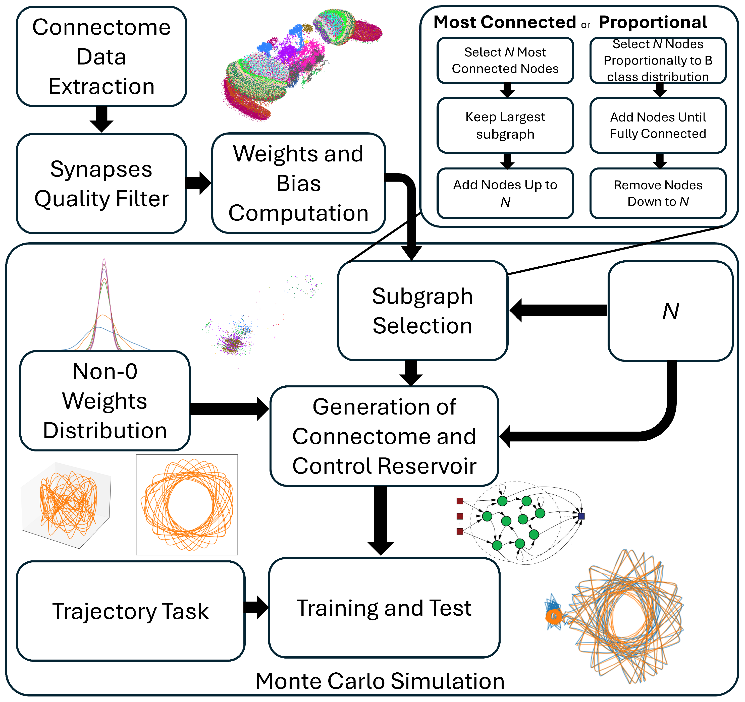
Figure 5.
(A) Sparsity and (B) variance of the non-zero weights as a function of the number of neurons selected in the reservoir. The probability density function of the extracted weight in the case of (C) the ‘most connected’ criterion and (D) the ‘proportional’ criterion.
Figure 5.
(A) Sparsity and (B) variance of the non-zero weights as a function of the number of neurons selected in the reservoir. The probability density function of the extracted weight in the case of (C) the ‘most connected’ criterion and (D) the ‘proportional’ criterion.
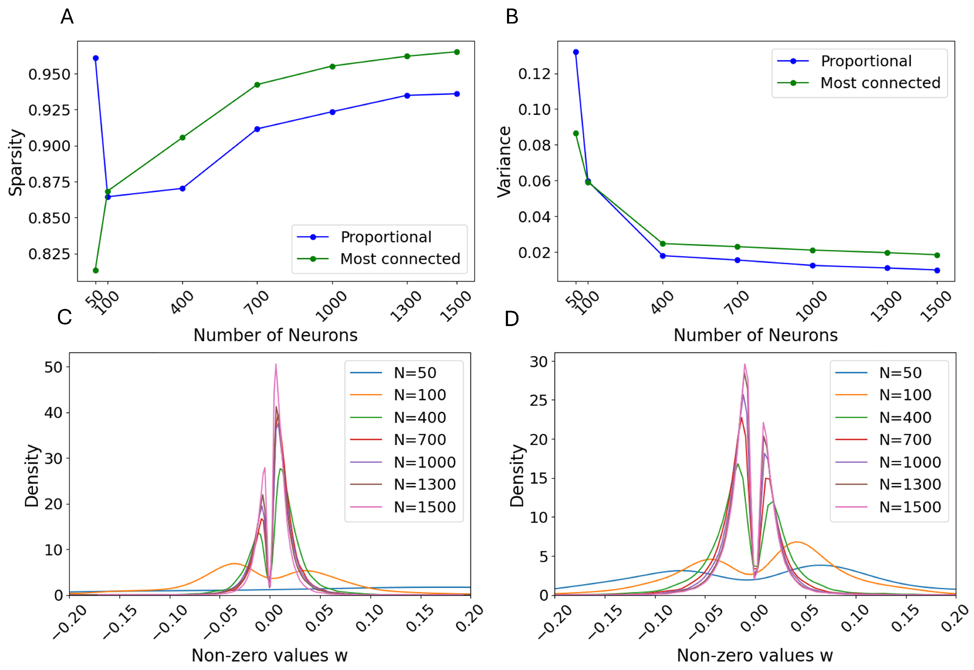
Figure 6.
3D scatterplot of selected reservoir and pie chart of the class division within such a reservoir in the case of: (A) ‘most connected’ criterion and , (B) ‘proportional’ criterion and , (C) ‘most connected’ criterion and , (D) ‘proportional’ criterion and , (E) ‘most connected’ criterion and , (F) ‘proportional’ criterion and , (G) ‘most connected’ criterion and , and (H) ‘proportional’ criterion and .
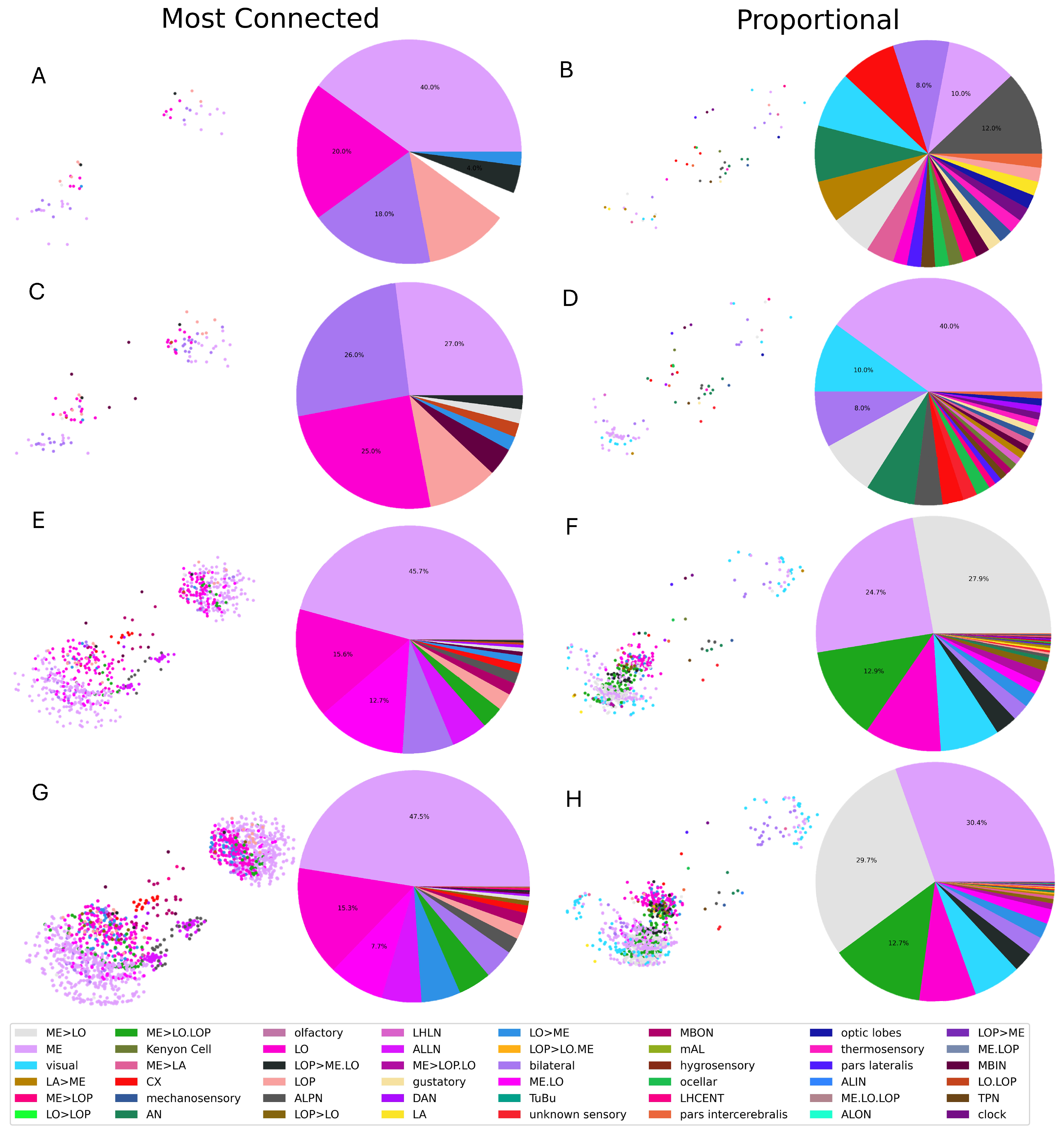
Figure 7.
Tology metrics of the selected reservoirs: (A) degree distribution for , (B) clustering coefficient distribution for , (C) shortest path distribution for , (D) degree distribution for , (E) clustering coefficient distribution for , (F) shortest path distribution for .
Figure 7.
Tology metrics of the selected reservoirs: (A) degree distribution for , (B) clustering coefficient distribution for , (C) shortest path distribution for , (D) degree distribution for , (E) clustering coefficient distribution for , (F) shortest path distribution for .
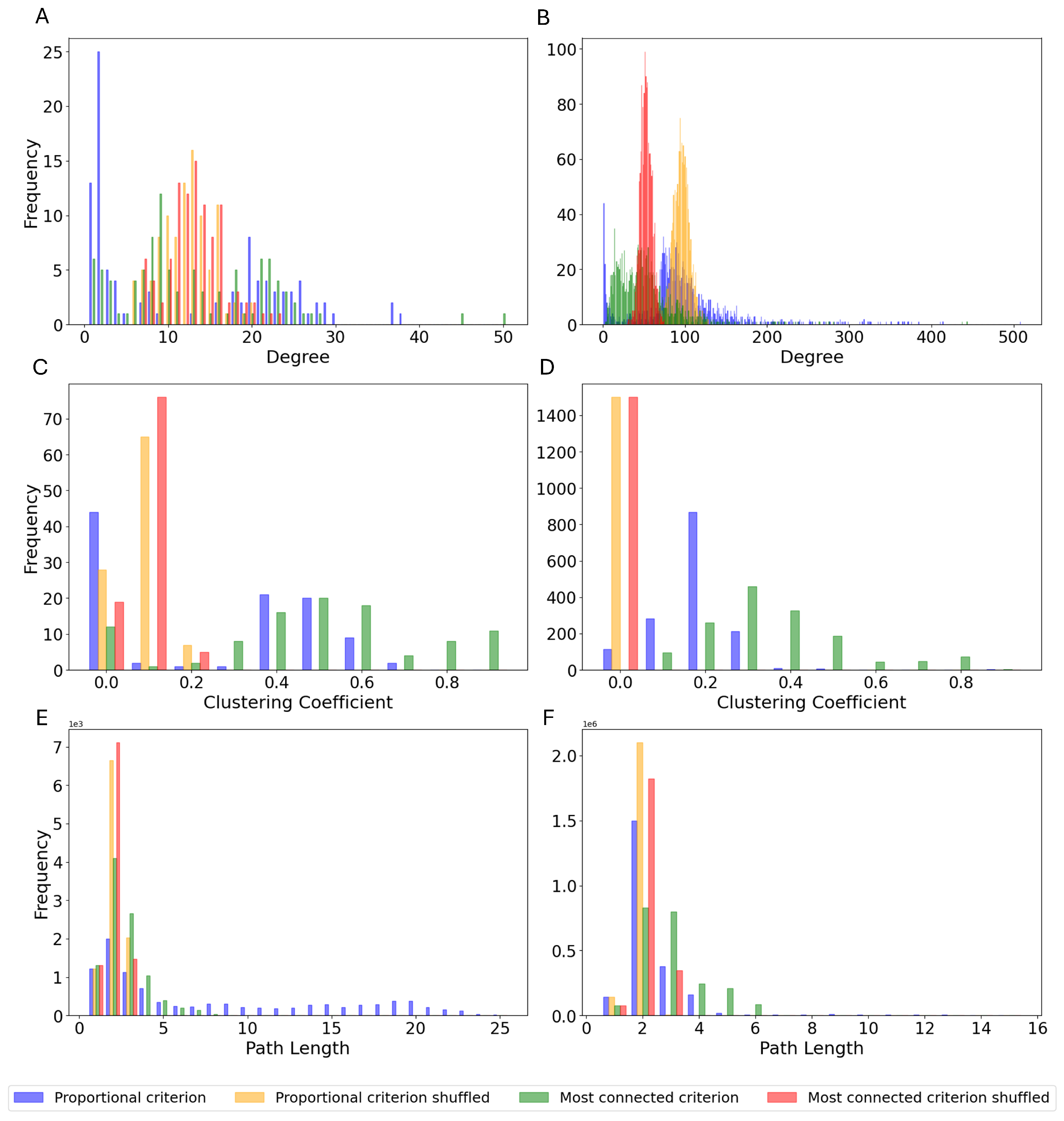
Figure 8.
The neuronal activation state of six random neurons during the washout in the case of (A) a classical reservoir with uniform non-zero weight distribution and (B) the reservoir extracted from the connectome. Example of the performance of the ESN on a single test trajectory in the case of , and a classical implementation obtained with a uniform distribution in the case of: (C) classical and (D) connectome-based reservoir and a 1-timestep prediction. (E) classical and (F) connectome-based reservoir and a 3-timestep prediction. (G) classical and (H) connectome-based reservoir and a 7-timestep prediction. (I) classical and (J) connectome-based reservoir and a 10-timestep prediction.
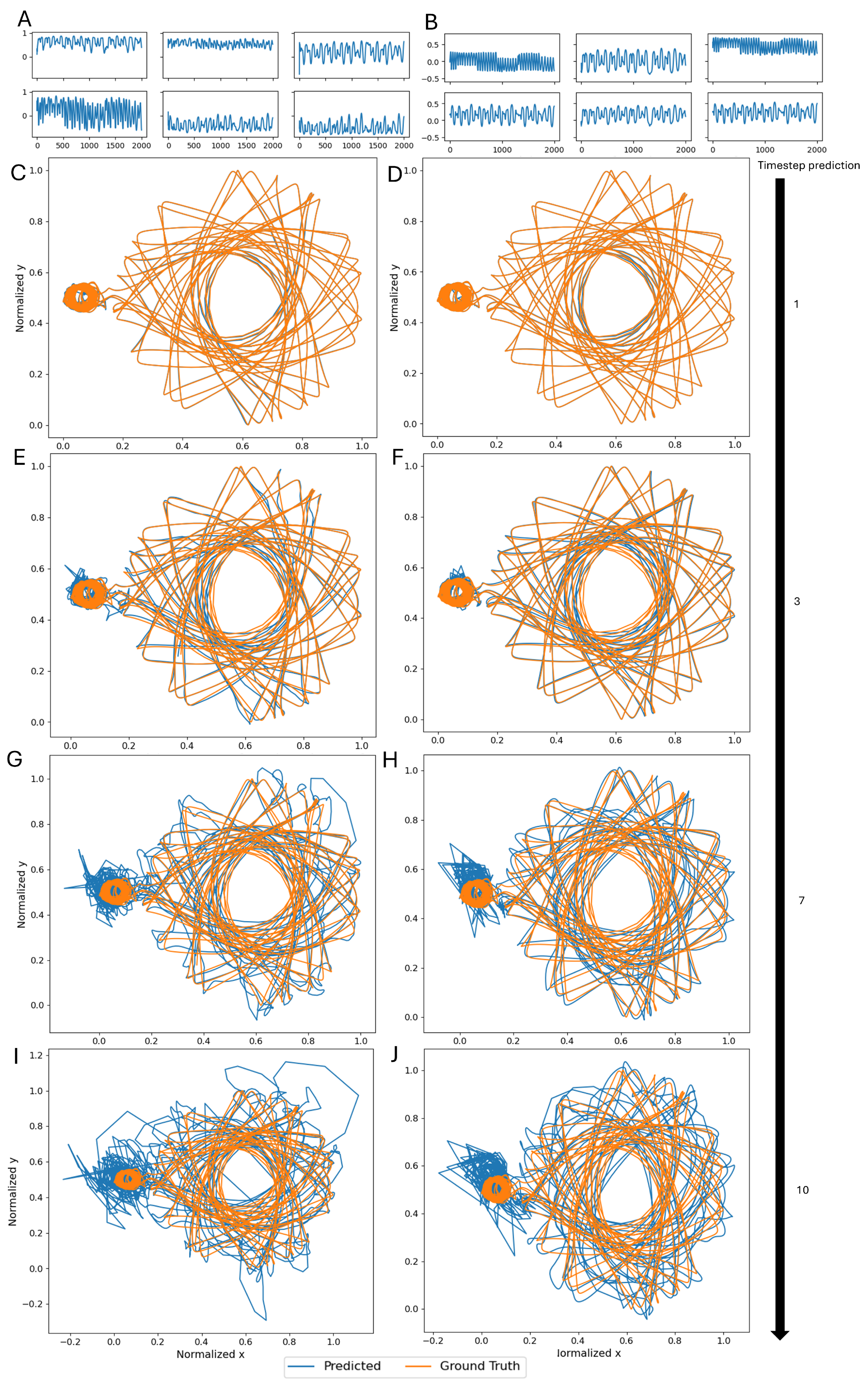
Figure 9.
Comparative results of ESN performance of train and test sets in the case of and . Connectome and classic refer to the connectome-based and random reservoirs, respectively. The selection criterion used for the extraction of neurons for the connectome-based ESN is ‘most connected’. Simulations have been performed for the following cases: (A) Gaussian and (B) uniform non-zero weight distribution with 1-timestep prediction for the classic reservoir, (C) Gaussian and (D) uniform non-zero weight distribution with 3-timestep prediction for the classic reservoir, (E) Gaussian and (F) uniform non-zero weight distribution with 7-timestep prediction for the classic reservoir, and (G) Gaussian and (H) uniform non-zero weight distribution with 10-timestep prediction for the classic reservoir.
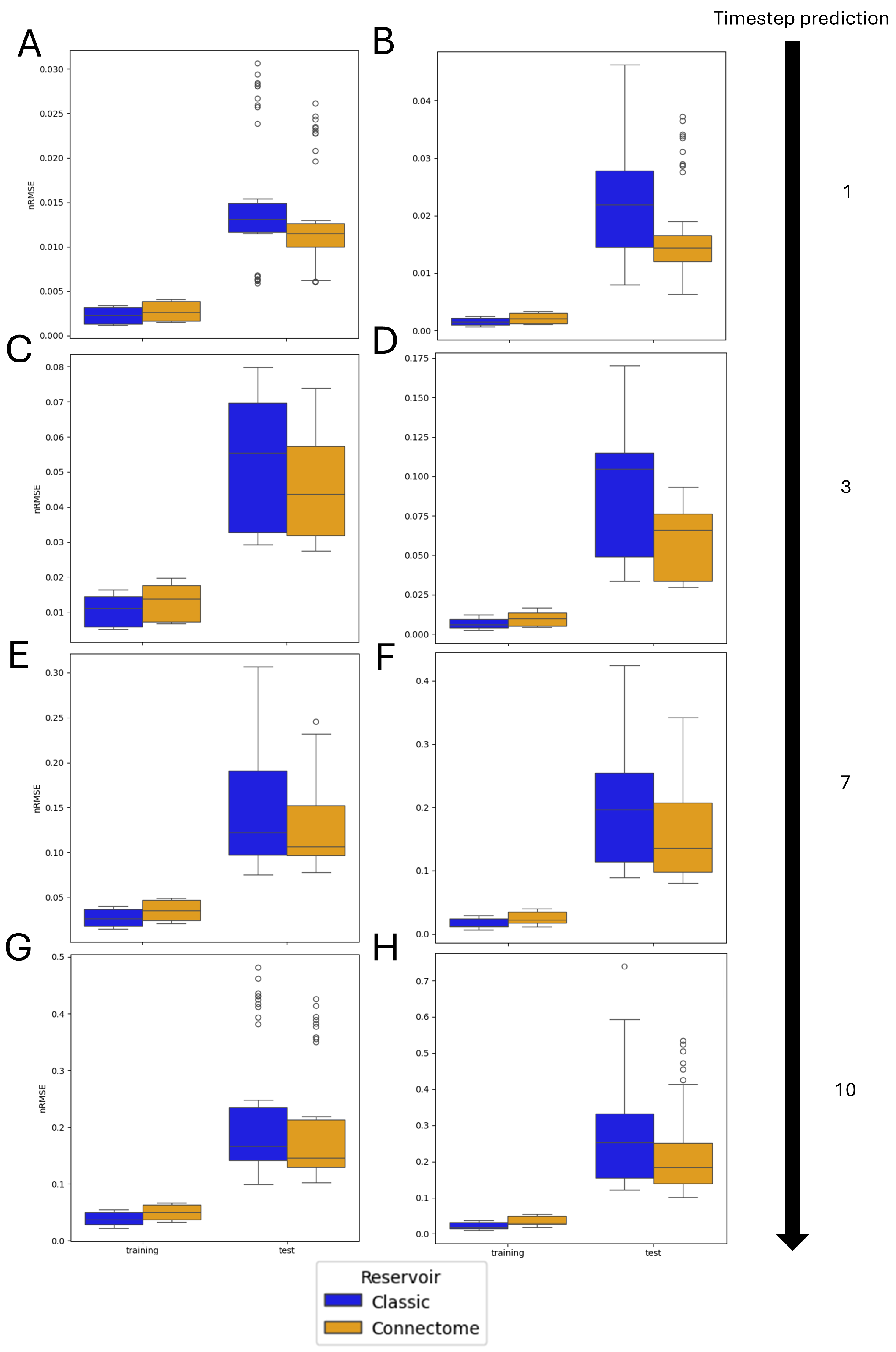
Figure 10.
Results on the test set as a function of reservoir size N and normalization factor using the ‘most connected’ selection criterion. Simulations have been performed for the following cases: (A) Gaussian and (B) uniform non-zero weight distribution for the classic reservoir with 1-timestep prediction, (C) Gaussian and (D) uniform non-zero weight distribution for the classic reservoir with 3-timestep prediction, (E) Gaussian and (F) uniform non-zero weight distribution for the classic reservoir with 7-timestep prediction, and (G) Gaussian and (H) uniform non-zero weight distribution for the classic reservoir with 10-timestep prediction. Error bars display the mean’s standard deviation. Statistically significant differences () under the Mann–Whitney–Wilcoxon test are indicated by the marker *, and no significance by the marker ∘ as follows: the control case of random topology and random weight has been tested against connectome-based topology and random weights distribution (left marker), connectome-based topology and extracted weights distribution (central marker), and random topology and extracted weights distribution (right marker).
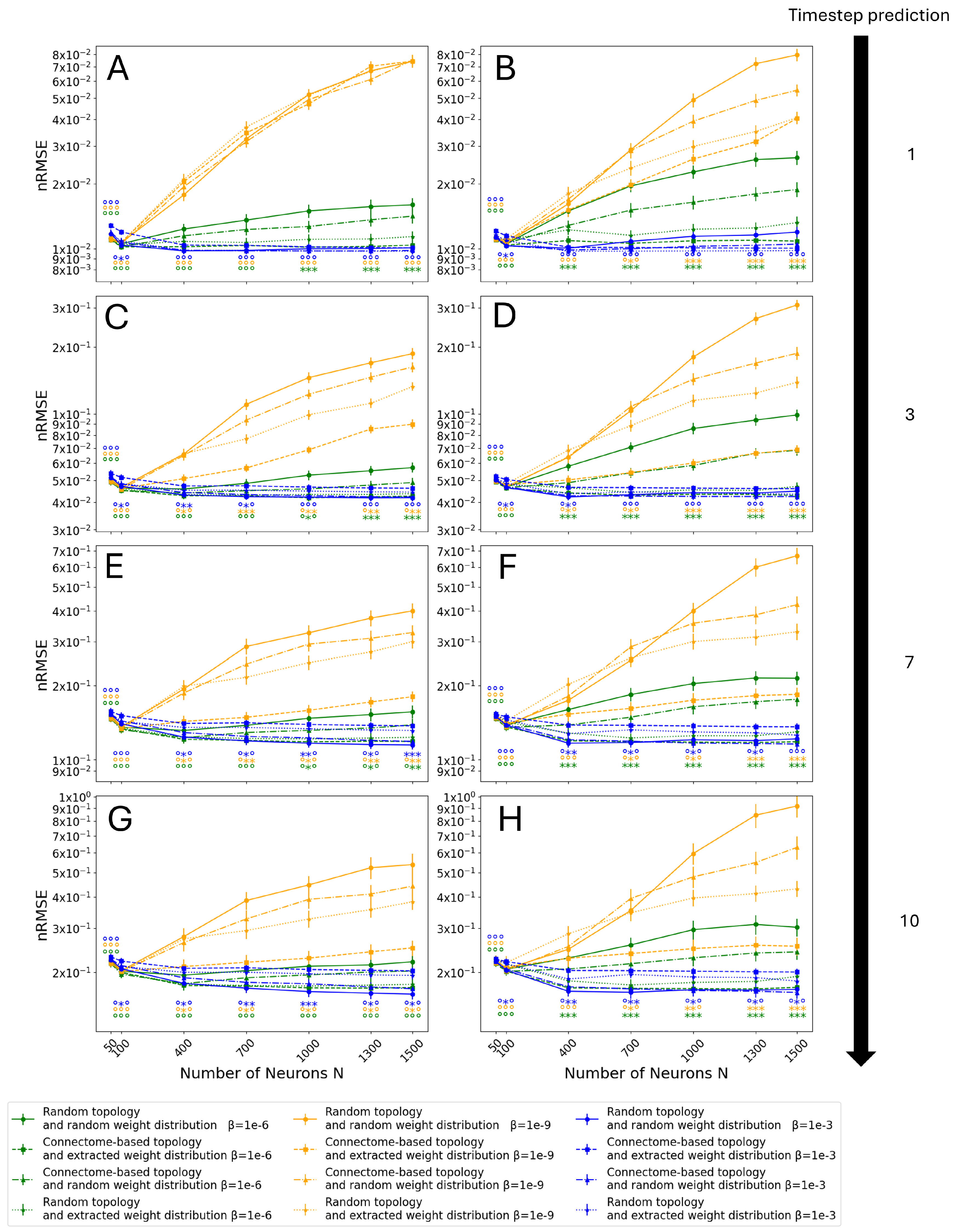
Figure 11.
Results on the test set as a function of reservoir size N and normalization factor using the ‘proportional’ selection criterion. Simulations have been performed for the following cases: (A) Gaussian and (B) uniform non-zero weight distribution for the classic reservoir with 1-timestep prediction, (C) Gaussian and (D) uniform non-zero weight distribution for the classic reservoir with 3-timestep prediction, (E) Gaussian and (F) uniform non-zero weight distribution for the classic reservoir with 7-timestep prediction, and (G) Gaussian and (H) uniform non-zero weight distribution for the classic reservoir with 10-timestep prediction. Error bars display the mean’s standard deviation. Statistically significant differences () under the Mann–Whitney–Wilcoxon test are indicated by the marker *, and no significance by the marker ∘ as follows: the control case of random topology and random weight has been tested against connectome-based topology and random weights distribution (left marker), connectome-based topology and extracted weights distribution (central marker), and random topology and extracted weights distribution (right marker).
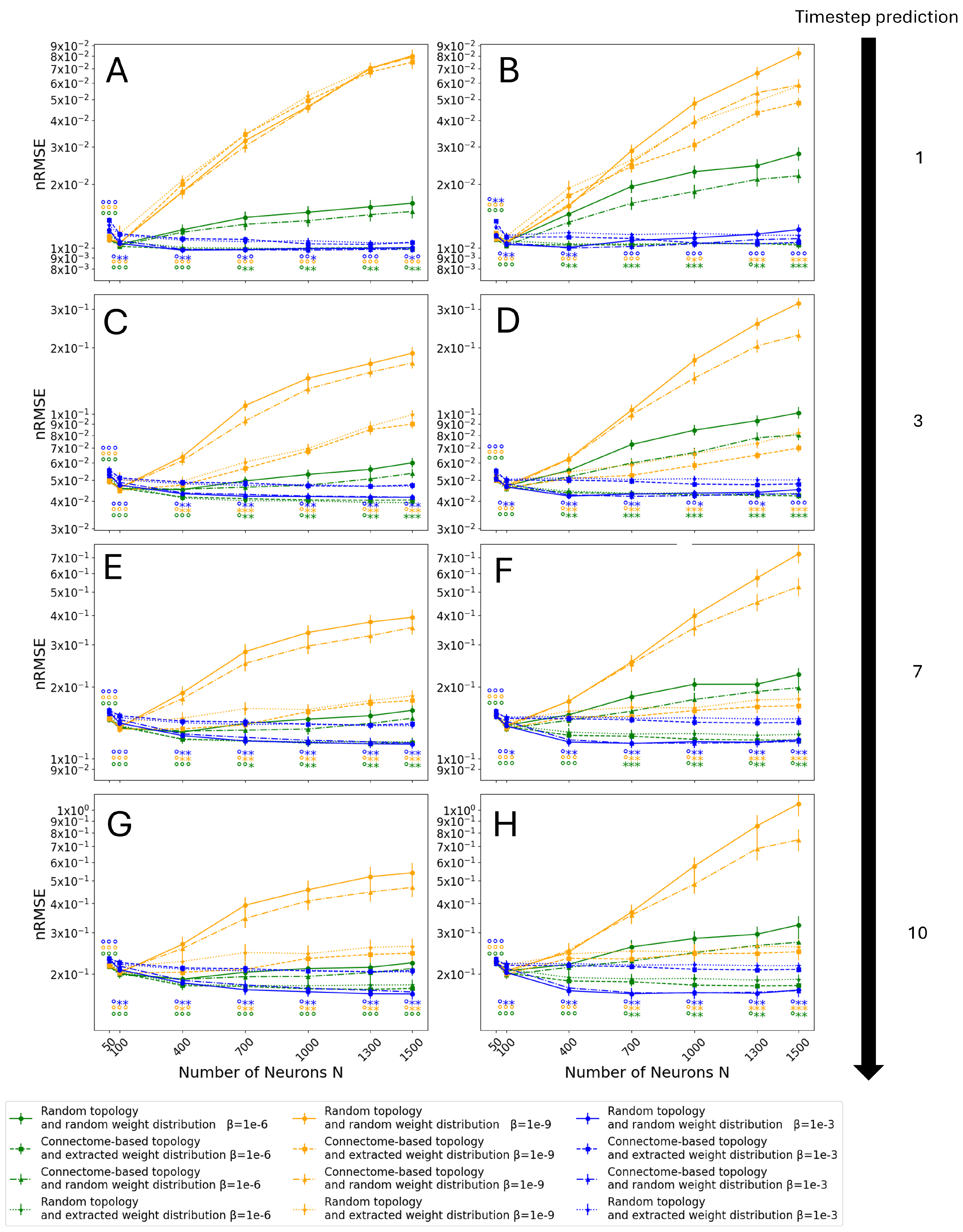
Figure 12.
Comparative results of ESN performance of training and test sets in the case of the whole connectome predicting one timestep into the future. The control architecture uses a uniform distribution of non-zero weights. Connectome and classic refer to the connectome-based and manually constructed reservoirs, respectively. The study has been performed in the following cases: (A) and (B) .
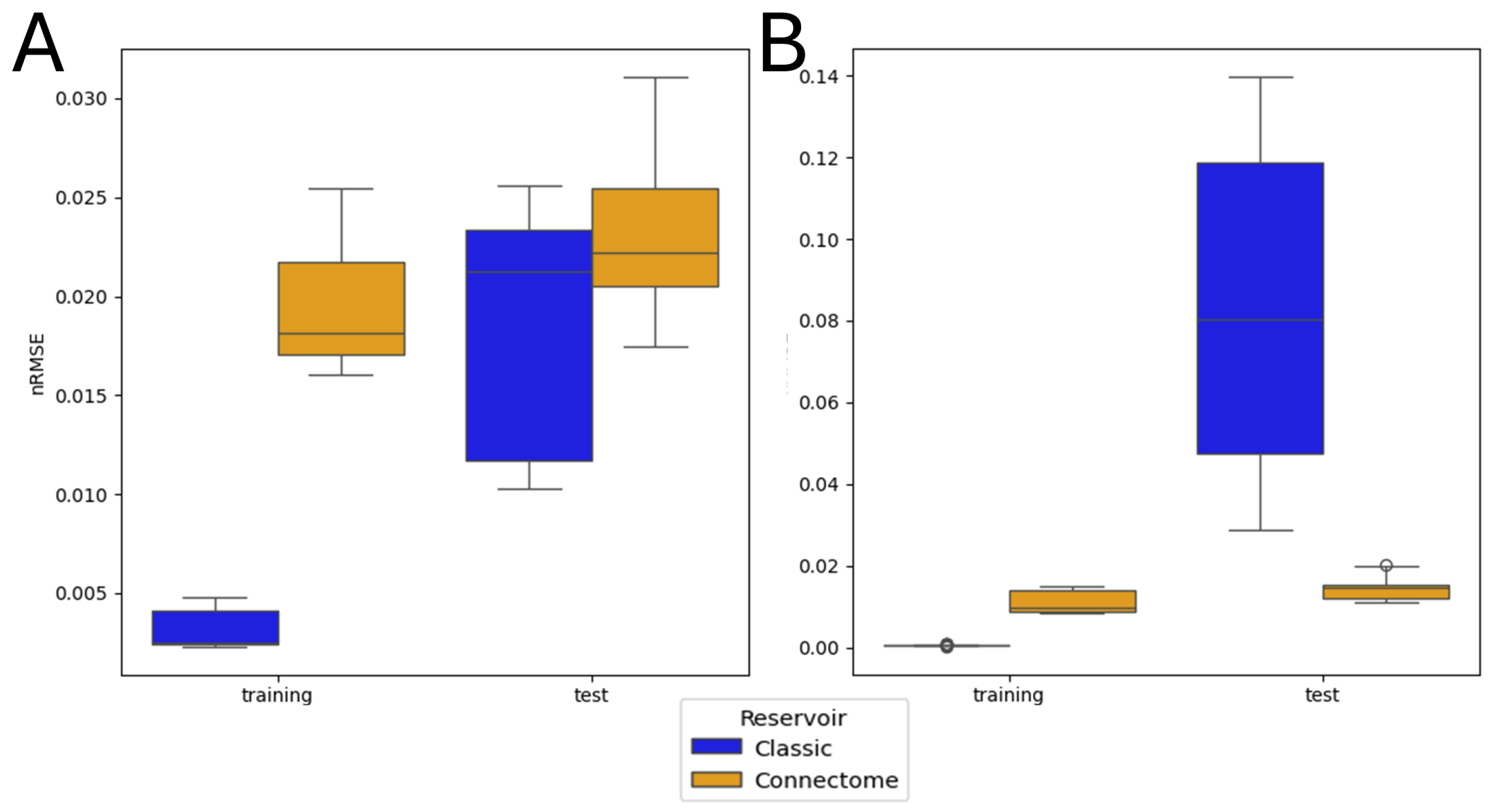

Table 1.
Neuronal class abbreviation, complete name, and brief function description for all classes present in the connectome.
Table 1.
Neuronal class abbreviation, complete name, and brief function description for all classes present in the connectome.
| Neuron Class | Full Name | Function | Neuron Class | Full Name | Function |
|---|---|---|---|---|---|
| CX | Central Complex | Motor control, navigation | Kenyon Cell | Kenyon Cell | Learning and memory |
| ALPN | Antennal Lobe Projection Neuron | Olfactory signal relay | LO | Lamina Output Neuron | Early visual processing |
| bilateral | Bilateral Neuron | Cross-hemisphere connections | ME | Medulla Neuron | Visual processing |
| ME>LOP | Medulla to Lobula Plate | Motion detection | ME>LO | Medulla to Lobula | Higher-order vision |
| LO>LOP | Lobula to Lobula Plate | Object motion detection | ME>LA | Medulla to Lamina | Visual contrast enhancement |
| LA>ME | Lamina to Medulla | Photoreceptor signal relay | ME>LO.LOP | Medulla to Lobula and Lobula Plate | Motion and feature integration |
| ALLN | Allatotropinergic Neuron | Hormonal regulation | olfactory | Olfactory Neuron | Detects airborne stimuli |
| DAN | Dopaminergic Neuron | Learning, reward, motivation | MBON | Mushroom Body Output Neuron | Readout of learned behaviors |
| ME>LOP.LO | Medulla to Lobula Plate and Lobula | Visual integration | LOP>ME.LO | Lobula Plate to Medulla and Lobula | Motion-sensitive feedback |
| LOP | Lobula Plate Neuron | Optic flow detection | LOP>LO.ME | Lobula Plate to Lobula and Medulla | Visual-motor integration |
| LOP>LO | Lobula Plate to Lobula | Motion-sensitive projection | LA | Lamina Neuron | First visual synaptic layer |
| AN | Antennal Neuron | Mechanosensory and olfactory processing | visual | Visual Neuron | General vision processing |
| TuBu | Tubercle Bulb Neuron | Connects brain to vision | LHCENT | Lateral Horn Centroid | Odor valence processing |
| ALIN | Antennal Lobe Interneuron | Olfactory modulation | mAL | Mushroom Body-associated Antennal Lobe Neuron | Olfactory-learning link |
| LHLN | Lateral Horn Local Neuron | Innate odor-driven behavior | ME.LO | Medulla and Lobula Neuron | General vision processing |
| mechanosensory | Mechanosensory Neuron | Touch, vibration detection | ME.LO.LOP | Medulla, Lobula, and Lobula Plate Neuron | Multi-layer vision processing |
| LO>ME | Lobula to Medulla | Visual feedback | hygrosensory | Hygrosensory Neuron | Detects humidity |
| pars lateralis | Pars Lateralis Neuron | Hormonal/circadian regulation | unknown sensory | Unknown Sensory Neuron | Uncharacterized sensory function |
| LO.LOP | Lobula and Lobula Plate Neuron | Motion and space awareness | ocellar | Ocellar Neuron | Light intensity detection |
| optic lobes | Optic Lobe Neuron | General vision processing | pars intercerebralis | Pars Intercerebralis Neuron | Hormonal regulation |
| ME.LOP | Medulla and Lobula Plate Neuron | Motion and edge detection | gustatory | Gustatory Neuron | Taste processing |
| ALON | Antennal Lobe Olfactory Neuron | Olfactory cue processing | MBIN | Mushroom Body Input Neuron | Learning circuit modulation |
| thermosensory | Thermosensory Neuron | Temperature sensing | clock | Clock Neuron | Circadian rhythm control |
| LOP>ME | Lobula Plate to Medulla | Motion-sensitive feedback | TPN | Transmedullary Projection Neuron | Optic lobes to brain |
Table 2.
Classification of neuron classes into input, intermediate, and output categories. The input neurons receive the input signal, whereas the output neurons are connected to the readout.
Table 2.
Classification of neuron classes into input, intermediate, and output categories. The input neurons receive the input signal, whereas the output neurons are connected to the readout.
| Type | Neuron Classes |
|---|---|
| Input | olfactory, visual, mechanosensory, hygrosensory, thermosensory, gustatory, ocellar, unknown sensory |
| Intermediate | CX, ALPN, LO, bilateral, ME, ME>LOP, ME>LO, LO>LOP, ME>LA, LA>ME, ME>LO.LOP, ALLN, LOP>ME.LO, LOP>LO.ME, LA, AN, ALIN, mAL, LHLN, ME.LO, ME.LO.LOP, LO>ME, optic lobes, ME.LOP, TPN |
| Output | MBON, DAN, LHCENT, clock, pars intercerebralis, pars lateralis, Kenyon Cell, ALON, LOP>ME, LOP>LO.ME, LOP>LO, LOP, TuBu |
Disclaimer/Publisher’s Note: The statements, opinions and data contained in all publications are solely those of the individual author(s) and contributor(s) and not of MDPI and/or the editor(s). MDPI and/or the editor(s) disclaim responsibility for any injury to people or property resulting from any ideas, methods, instructions or products referred to in the content. |
© 2025 by the authors. Licensee MDPI, Basel, Switzerland. This article is an open access article distributed under the terms and conditions of the Creative Commons Attribution (CC BY) license (http://creativecommons.org/licenses/by/4.0/).
Copyright: This open access article is published under a Creative Commons CC BY 4.0 license, which permit the free download, distribution, and reuse, provided that the author and preprint are cited in any reuse.


