Assessment of Anesthetic Depth Through EEG Mode Decomposition Using Singular Spectrum Analysis

1. Introduction

In patients under general anesthesia (GA), electroencephalography (EEG) results change significantly due to the hypnotic effects of anesthetic drugs, causing these patients to transition from an awake state to a state of unconsciousness [3,4,5,6]. As a result, monitoring and quantifying these changes in EEG results has facilitated the development of technologies to assess the depth of anesthesia, aiding in its management [7,8,9]. Since the late 1990s, commercial devices such as the bispectral index (BIS) monitor (Medtronic, Dublin, Ireland) and SEDLine (Masimo, Irvine, USA), which enable spectral analysis of EEG results, have become available. These devices use fast Fourier transform technology to detect changes in the frequency components of EEG results, calculate parameters related to the depth of anesthesia, and visualize the hypnotic effects of general anesthetics through changes in the power spectrum presented as density spectral array color maps. However, techniques that analyze changes in the frequency components of electroencephalographic signals during general anesthesia and translate them into quantitative assessments of anesthetic depth are still not fully established, as they are influenced by variables such as the type of anesthetic agent and patient age, and thus remain an area with considerable potential for further development.

While the Fourier transform is a powerful tool for analyzing stationary signals, it falls short for non-stationary signals. In such cases, the discrete wavelet transform is often used. This method, like the Fourier transform, decomposes data based on a basis set and is used in multi-resolution analysis [10]. However, with wavelet transforms, the time and frequency resolution changes depending on the scale of the basis function, and it is necessary to appropriately choose the type of wavelet and parameters (such as the number of scales and the range of analysis); this often requires experience and extensive trial and error, making this a significant drawback in EEG analysis.

Recently, techniques combining modal decomposition and the Hilbert transform have been investigated as new alternatives to the fast Fourier transform. EEG is considered to show the collection of micro-electrical activities of neuronal groups in the cerebral cortex. Mode decomposition methods appropriately decompose these electrical activities, capturing them as the activity of virtual functional groups of cells and observing their modes. On the other hand, the Hilbert transform is a signal processing technique in the complex domain that shifts the phase by 90 degrees to obtain the instantaneous amplitude (IA) and frequency (IF). The Hilbert–Huang Transform, which combines empirical mode decomposition (EMD) with the Hilbert transform, has been reported to be effective for analyzing non-stationary time series and impulse data [11]. We have also published research in which we applied the Hilbert–Huang Transform to EEGs during propofol-induced GA [2]. Furthermore, we have evaluated the usefulness of various modal decomposition methods for EEG analysis during sevoflurane total anesthesia, including variational mode decomposition (VMD) [2,12], which decomposes EEGs into narrow-band mode functions, and the empirical wavelet transform (EWT), which uses Meyer wavelets to decompose into narrow frequency bands and assess them as precise band-pass filters for EEG decomposition [13,14].

In this study, we introduce a novel method for mode decomposition of time series data using singular spectrum analysis (SSA) [15,16]. This method is particularly suitable for non-stationary signals and does not require the pre-specification of bases. SSA involves transforming one-dimensional time series data into a matrix via a one-to-one mapping, then applying singular value decomposition (SVD) to the matrix [17]. SSA extends the spectral decomposition, which involves eigenvalues and eigenspectra of Hermitian matrices in linear algebra, to arbitrary rectangular matrices. It involves the use of SVD to extract trends, periodic components, and noise from data, such as time series, demonstrating its strength in analyzing non-stationary signals. In this research, we combine modal decomposition via SSA with the Hilbert transform for frequency analysis to investigate its utility for extracting EEG characteristics during GA with inhalational sevoflurane.

2. Theoretical background, methods, and materials

2.1. Algorithm for SVD

2.1.1. Singular values, singular vectors, and SVD of a rectangular matrix

Let $\mathit{M}$ be a matrix over ${\mathit{K}}^{m\times n}$. The adjoint matrix of $\mathit{M}$ is denoted by ${\mathit{M}}^{\mathrm{*}}$. For a matrix $\mathit{M}$ of size $m\times n$ with complex numbers as its elements, ${\mathit{M}}^{\mathrm{*}}$ is the $n\times m$ matrix obtained by transposing $\mathit{M}$ and taking the complex conjugate of its elements. If $\mathit{M}$ consists entirely of real numbers, finding the adjoint of $\mathit{M}$ is equivalent to finding its transpose.

When there exists a pair of unit vectors $\mathit{u}$ in ${\mathit{K}}^m$ and $\mathit{v}$ in ${\mathit{K}}^n$ that satisfy the conditions

$$\mathit{M}\mathit{v}=\mathit{\sigma }\mathit{u} \mathrm{and} {\mathit{M}}^{\mathit{*}}\mathit{u}=\mathit{\sigma }\mathit{v}$$

(1)

for some non-negative real number $\mathit{\sigma }$, this real number $\mathit{\sigma }$ is called the singular value of matrix $\mathit{M}$ (corresponding to vectors $\mathit{u}$ and $\mathit{v}$). Furthermore, vectors $\mathit{u}$ and $\mathit{v}$ are called the left singular vector and right singular vector of $\mathit{M}$, respectively.

In the decomposition

$$\mathit{M}=\mathit{U}{\sum \mathit{V}}^{\mathrm{*}}$$

(2)

the diagonal components of $\sum$ are equal to the singular values of $\mathit{M}$, and the column vectors of the unitary matrices $\mathit{U}$ and $\mathit{V}$ consist of the left singular vectors and right singular vectors of matrix $\mathit{M}$, respectively. Here, a unitary matrix is defined as a complex square matrix $\mathit{U}$ that satisfies

$${\mathit{U}}^{\mathrm{*}}\mathit{U}=\mathit{U}{\mathit{U}}^{\mathrm{*}}=\mathit{I}$$

(3)

where $\mathit{I}$ is the identity matrix, and ${\mathit{U}}^{\mathrm{*}}$ is the adjoint matrix of $\mathit{U}$ (${\mathit{U}}^{\mathrm{*}}={\mathit{U}}^{\mathrm{T}}$ for real matrices).

Thus, for real matrices, the adjoint is simply the transpose, and the real unitary matrices are equivalent to orthogonal matrices. When extended to the complex number field, these become unitary matrices. Accordingly, an $m\times n$ matrix $\mathit{M}$ has at least one and at most $d=min(m, n)$ distinct singular values. There always exists a unitary basis in ${\mathit{K}}^{\mathrm{m}}$ consisting of the left singular vectors of $\mathit{M}$, and there always exists a unitary basis in ${\mathit{K}}^{\mathrm{n}}$ consisting of the right singular vectors of $\mathit{M}$.

2.1.2. SVD of EEG

Consider the time series of EEG voltage (in microvolts) sampled at 128 Hz for 3 seconds (N + 1 = 384), denoted by

$${\mathit{F}=\{x}_0,x_1,x_2,\dots \dots ,x_{N-1}\}$$

(4)

To apply SSA to the EEG time series data, first, set the window length to $K=256$ (corresponding to 2 seconds of data) and extract 128 columns (L = 128) of time series data by sliding the window. Then, construct a matrix known as a Hankel matrix in the following form:

$$\mathbf{X}=\left(\begin{array}{cccc}{x}_0& x_1& \dots & x_{K-1}\\ x_1& x_2& ⋮& x_K\\ ⋮& ⋮& \ddots & ⋮\\ x_{L-1}& x_L& \dots & x_{N-1}\end{array}\right)$$

(5)

The first row consists of $K$ data points from $x_0$ to $x_{K-1}$, the second row consists of K data points from $x_1$ to $x_K$, the third row consists of $K=256$ data points from $x_2$ to $x_{K+1}$, and so on, until the right end of the sliding window reaches the last data point of the EEG time series, $x_{N-1}$. This process is repeated 128 times ($L=N-K+1$, 128 = 383 – 256 $+ 1$). In the trajectory matrix, the same components appear from the top right to the bottom left, which is a characteristic of a Hankel matrix. The columns of X are called L-lagged vectors, and the rows are called K-lagged vectors.

In the second step, the trajectory matrix is decomposed using SVD.

$$\mathit{X}=\mathit{U}{\sum \mathit{V}}^{\mathrm{T}}$$

(6)

Here, $\mathit{U}$ is an $L\times L$ unitary matrix (i.e., $\mathit{U}{\mathit{U}}^{\mathrm{*}}=\mathit{I}$) containing an orthonormal set of left singular vectors of $\mathit{X}$. $\sum$ is an $L\times K$ rectangular diagonal matrix that contains the d (where $d=min(K, L)$) singular values of $\mathit{X}$ in descending order. $\mathit{V}$ is a $K\times K$ unitary matrix containing an orthonormal set of right singular vectors of $\mathit{X}$.

Since $\sum$ has nonzero entries only on its diagonal, the matrix product $\mathit{U}{\sum \mathit{V}}^{\mathrm{T}}$ can be expanded as a sum of rank-one matrices. Then, $\mathit{X}$ can be decomposed as

$$\mathit{X}={\sigma }_0{\mathit{u}}_0{\mathit{v}}_0^{\mathrm{T}}+{\sigma }_1{\mathit{u}}_1{\mathit{v}}_1^{\mathrm{T}}+\dots ..+{\sigma }_{d-1}{\mathit{u}}_{d-1}{\mathit{v}}_{d-1}^{\mathrm{T}}$$

(7)

In this decomposition, the weights corresponding to the singular values determine the contribution of each basis, and the magnitude of the singular values indicates the relative importance of each basis. Equivalently, using summation notation, this decomposition can be expressed as follows:

$$\mathit{X}=\sum _{i=0}^{d-1}{\mathsf{\sigma }}_i{\mathit{u}}_i {\mathit{v}}_i^{\mathrm{T}} \equiv \sum _{i=0}^{d-1}{\mathit{X}}_i$$

(8)

Here, the parameter $d(\le L)$ is the rank of the trajectory matrix, ${\mathsf{\sigma }}_i$ denotes the i-th singular value of $\mathit{X}$, and ${\mathit{u}}_i$ and ${\mathit{v}}_i$ are the corresponding left and right singular vectors, given by the i-th columns of $\mathit{U}$ and $\mathit{V}$, respectively. The set {${\mathit{u}}_i$, ${\sigma }_i$, ${\mathit{v}}_i$} is called the $i$-th eigentriple of the SVD. In this way, applying SVD to the trajectory matrix decomposes it into d matrices ${\mathit{X}}_i={\mathsf{\sigma }}_i{\mathit{u}}_i{\mathit{v}}_i^{\mathrm{T}}$, where the significant components have larger singular values ${\sigma }_{\mathrm{i}}$.

In the case of dimensionality reduction, only the components that need to be retained are kept and used for reconstruction. For example, in noise reduction, one can look at the singular values and retain only those above a certain threshold. In the case of EEG analysis, grouping all components into several categories can be used for feature extraction.

2.1.3. Time series component separation and grouping

Up to this point, the EEG time series $\mathit{F}$ has been embedded into a sequence of $L$-lagged vectors, thereby forming the trajectory matrix of $\mathit{F}$. SVD is then applied to this matrix, resulting in a set of elementary matrices whose sum reconstructs the original trajectory matrix. In an ideal scenario, the time series $\mathit{F}$ can be decomposed into a sum of mutually separable components, $\mathit{F}=\sum _{\mathit{j}}{\mathit{F}}^{\left(j\right)}$. By appropriately grouping the corresponding elementary matrices ${\mathit{X}}_i$, the trajectory matrix can be expressed as

$$\mathit{X}=\sum _{k\in \mathrm{S}}{\mathit{X}}_k+\sum _{l\in \mathrm{T}}{\mathit{X}}_l+\dots =\sum _j{\mathit{X}}^{\left(j\right)}$$

(9)

where $S$ and $T$ are mutually exclusive index sets, and ${\mathit{X}}^{\left(j\right)}$ represents the trajectory matrix corresponding to the component ${\mathit{F}}^{\left(j\right)}$. Each ${\mathit{X}}^{\left(j\right)}$ preserves the Hankel structure of the original trajectory matrix. The reconstructed time series ${\mathit{F}}^{\left(\tilde{j}\right)}$ is then obtained via diagonal averaging, in which the elements of ${\mathit{X}}^{\left(j\right)}$ are averaged along anti-diagonals extending from the upper right to the lower left of the matrix.

The element ${\tilde{\mathit{x}}}_{(p,q)}$ of the reconstructed matrix ${\tilde{\mathit{X}}}^{\left(j\right)}$, with $s=p+q$, $K=256\ge L=128$, and $s=0, 1, \dots ,N-1,$ is defined by the diagonal averaging operation as follows:

$${{\mathit{F}}_{\mathit{S}}}^{\left(j\right)}\equiv {\tilde{\mathit{x}}}_{(p,q)}=\left\{\begin{array}{c}{\displaystyle \frac{1}{s+1}}{\sum }_{p=0}^s{{\tilde{\mathit{x}}}^{\left(j\right)}}_{(p, s-p)} (0\le s\le L-2)\\ {\displaystyle \frac{1}{L}}{\sum }_{p=0}^{L-1}{{\tilde{\mathit{x}}}^{\left(j\right)}}_{\left(p, s-p\right)} \left(L-2\le s\le K-1\right)\\ {\displaystyle \frac{1}{L+K-s-1}}{\sum }_{p=s-K+1}^{L-1}{{\tilde{\mathit{x}}}^{\left(j\right)}}_{(p, s-p)} (K\le s\le K + L - 2)\end{array}\right.$$

(10)

Each grouped time series, obtained by summing selected elementary components, is treated as an intrinsic mode function (IMF), to which the Hilbert transform is applied.

2.1.4. Computer Programming for SVD

A sample program for matrix calculations for SVD is provided in Appendix A. The Python program code for SVD is shown in Table A1 (Additional file 1), and the Java program code is shown in Table A2 (Additional file 2).

2.1.5. Hilbert transform

The Hilbert transform is applied to the IMF components, denoted by $imf\left(t\right)$, and the analytic signal $z\left(t\right)$ is obtained as follows [1,2,11,18,19,20,21]:

$\mathbf{A}\mathbf{n}\mathbf{a}\mathbf{l}\mathbf{y}\mathbf{t}\mathbf{i}\mathbf{c} \mathbf{s}\mathbf{i}\mathbf{g}\mathbf{n}\mathbf{a}\mathbf{l} z\left(t\right)=imf\left(t\right)+iH\left[imf\left(t\right)\right]=a\left(t\right)e^{i\int \mathit{\omega }\left(t\right)dt}$		(11)
in which $a\left(t\right)=\sqrt{{imf\left(t\right)}^2+{H\left[imf\left(t\right)\right]}^2}$	Instantaneous amplitude (IA)	(12)
$\omega \left(t\right)={{\displaystyle \frac{t}{dt}}[tan}^{-1}\left({\displaystyle \frac{\mathrm{H}\left[imf\right(t)}{imf\left(t\right)}}\right)]$	Instantaneous frequency (IF)	(13)
$h\left(\mathit{\omega }\right)=\int H(\omega , t)dt$	Marginal Hilbert spectrum	(14)

where $\omega \left(t\right)$ and $a\left(t\right)$ are the IF and the IA of the IMF used to obtain a time–frequency distribution for signal $imf\left(t\right)$and the Hilbert amplitude spectrum $H(\omega ,t)$.

2.3. Anesthesia Management and Data Acquisition

This study used a previously reported [2] and publicly available dataset of EEG data from patients under sevoflurane GA (ten minutes until awakening in ten cases of GA, https://github.com/teijisw/EEG_DataSet/tree/master/general_anesth_sevoflurane) (Additional File 3). The original data acquisition was performed using EEG Analyzer software [22] (EEG Analyzer ver. 54_GP, http://anesth-kpum.org/blog_ts/?p=3169) linked to a VISTA A-3000 BIS monitor with a BIS Quatro sensor [22]. For more details on patient information, anesthesia management, and data acquisition, such as the raw EEG, BIS, 95% spectral edge frequency (SEF₉₅), total power (TP), and absolute power derived from electromyography in the 70–110 Hz range (EMG_low), please refer to our previous report [2].

2.4. Data Processing and Statistics

The changes in the various EEG parameters between two time points were compared statistically by conducting Kruskal‒Wallis tests with SPSS Statistics (28.0.1.0, IBM Corp., Armonk, NY, USA), and p-values < 0.05 were considered statistically significant. Multiple linear regression (MLR) analysis of the BIS and IMF parameters was performed using the scikit-learn [17] and StatsModels libraries in Python (ver. 3.8), as in our recent reports [23,24].

3. Results

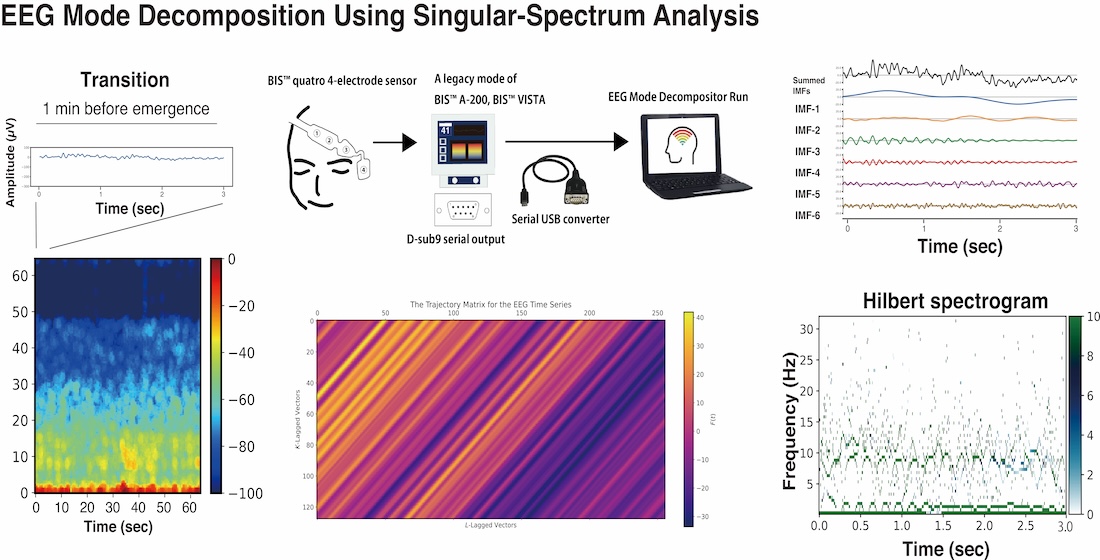
Using an EEG dataset from 10 cases of general anesthesia with sevoflurane, mode decomposition was performed using SAA. This dataset consisted of single-channel frontal EEG recordings from a BIS monitor, spanning 10 minutes from the maintenance phase of general anesthesia to the emergence phase.

3.1. Case Analysis of SSA Application

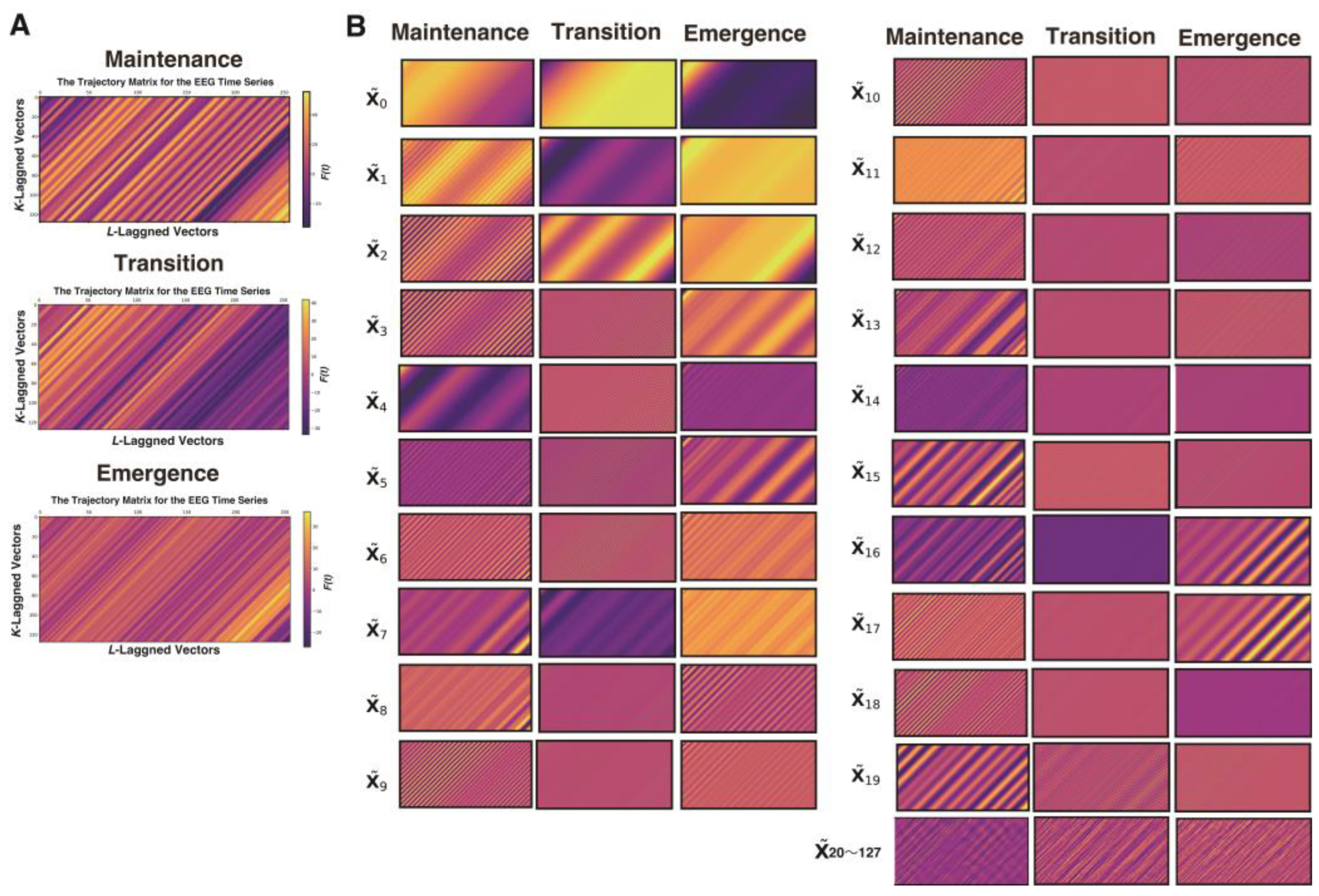
First, we present the SAA that was conducted using the EEG data acquired from Patient #1 (a 54-year-old female who was diagnosed with IgA nephropathy and underwent palatine tonsillectomy) [2] anesthetized with sevoflurane. We analyzed 3 s long epochs of EEG data that were recorded at 128 Hz during three distinct phases of GA up to the point of emergence: the maintenance (10 min before emergence), transition (1 min before emergence), and emergence phases. From each 3-second segment containing 384 data points, a trajectory matrix of 128 rows × 256 columns was constructed using a 2-second window (256 data points), shifted by 1 data point at a time. Then, a process was applied to group the elementary matrices into several component sets and subsequently reconstruct each set into a time series (Figure 1).

A process was applied to convert each elementary matrix into a Hankel matrix and subsequently reconstruct it into a time series. The color visualization of the trajectory matrix of the EEG time series highlights the characteristics of the elementary matrices. For example, ${\mathit{X}}_0^{~}$ and ${\mathit{X}}_1^{~}$ changed very gradually throughout the entire time series and can be interpreted as trend components. ${\mathit{X}}_2^{~}$ and ${\mathit{X}}_3^{~}$ also often exhibited slow periodicity. In the range from approximately ${\mathbf{X}}_4^{~}$ to ${\mathbf{X}}_9^{~}$, periodicity was frequently visible, whereas from ${\mathit{X}}_{10}^{~}$ onward, the components consisted of fine waves with high frequencies.

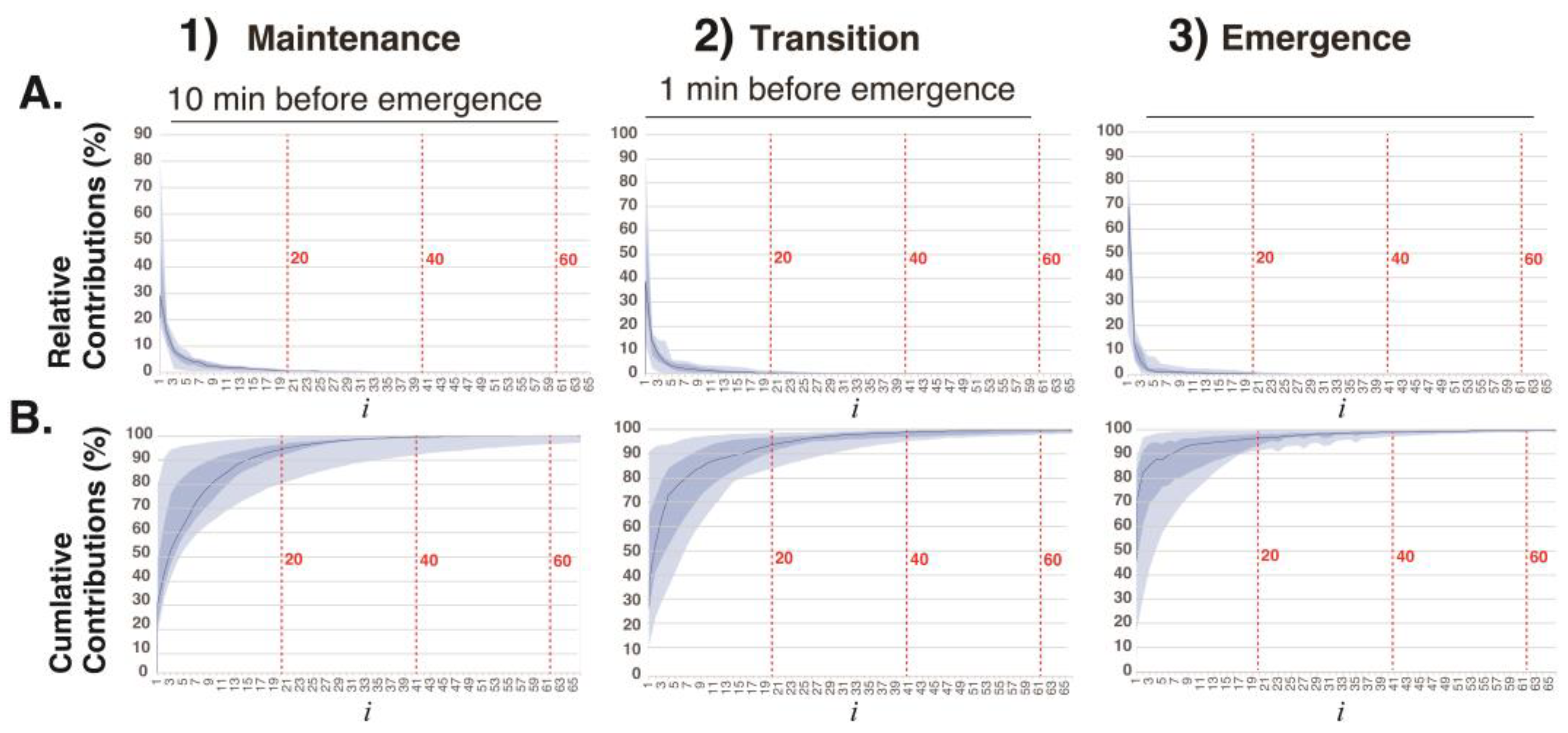
The relative contributions

$${\displaystyle \frac{{\sigma }_i^2}{\sum _{k=0}^{d-1}{\sigma }_k^2}}$$

(15)

and cumulative contributions

$${\displaystyle \frac{\sum _{j=0}^i{\sigma }_j^2}{\sum _{k=0}^{d-1}{\sigma }_k^2}}$$

(16)

of the first 64 elementary matrices ${\mathit{X}}_i$in the decomposition $\mathit{X}$=$\sum _{i=0}^{d-1}{\mathit{X}}_i$ obtained via SVD of 3-second EEG segments in the three phases of general anesthesia (Figure 2). The elementary matrices ${\mathit{X}}_0$ and ${\mathit{X}}_1$ contributed 22% and 21%, respectively, to the overall decomposition of $\mathrm{X}$. The first 20 elementary matrices together accounted for 97% of the total contribution. In this study, the 128 matrices obtained via SAA were grouped into six sets: 0–1, 2–3, 4–6, 7–9, 10–19, and 20–127. The matrices within each group were summed:

$${\tilde{\mathit{X}}}_0〜{\tilde{\mathit{X}}}_1, {\tilde{\mathit{X}}}_2〜{\tilde{\mathit{X}}}_3, {\tilde{\mathit{X}}}_4〜{\tilde{\mathit{X}}}_6, {\tilde{\mathit{X}}}_7〜{\tilde{\mathit{X}}}_9, {\tilde{\mathit{X}}}_{10}〜{\tilde{\mathit{X}}}_{19}, {\tilde{\mathit{X}}}_{20}〜{\tilde{\mathit{X}}}_{127}$$

(17)

$${\tilde{\mathit{X}}}^{(\mathrm{I}\mathrm{M}\mathrm{F}-1)}={\tilde{\mathit{X}}}_0+{\tilde{\mathit{X}}}_1\Rightarrow {\tilde{\mathit{F}}}^{(\mathrm{I}\mathrm{M}\mathrm{F}-1)}={\tilde{\mathit{F}}}_0+{\tilde{\mathit{F}}}_1$$

(18)

$${\tilde{\mathit{X}}}^{(\mathrm{I}\mathrm{M}\mathrm{F}-2)}={\tilde{\mathit{X}}}_2+{\tilde{\mathit{X}}}_3\Rightarrow {\tilde{\mathit{F}}}^{(\mathrm{I}\mathrm{M}\mathrm{F}-2)}={\tilde{\mathit{F}}}_2+{\tilde{\mathit{F}}}_3$$

(19)

$${\tilde{\mathit{X}}}^{(\mathrm{I}\mathrm{M}\mathrm{F}-3)}={\tilde{\mathit{X}}}_4+{\tilde{\mathit{X}}}_5+{\tilde{\mathit{X}}}_6\Rightarrow {\tilde{\mathit{F}}}^{(\mathrm{I}\mathrm{M}\mathrm{F}-3)}={\tilde{\mathit{F}}}_4+{\tilde{\mathit{F}}}_5+{\tilde{\mathit{F}}}_6$$

(20)

$${\tilde{\mathit{X}}}^{(\mathrm{I}\mathrm{M}\mathrm{F}-4)}={\tilde{\mathit{X}}}_7+{\tilde{\mathit{X}}}_8+{\tilde{\mathit{X}}}_9\Rightarrow {\tilde{\mathit{F}}}^{(\mathrm{I}\mathrm{M}\mathrm{F}-4)}={\tilde{\mathit{F}}}_7+{\tilde{\mathit{F}}}_8+{\tilde{\mathit{F}}}_9$$

(21)

$${\tilde{\mathit{X}}}^{(\mathrm{I}\mathrm{M}\mathrm{F}-5)}={\tilde{\mathit{X}}}_{10}+\cdots +{\tilde{\mathit{X}}}_{19}\Rightarrow {\tilde{\mathit{F}}}^{\left(\mathrm{I}\mathrm{M}\mathrm{F}-5\right)}={\tilde{\mathit{F}}}_{10}+\cdots +{\tilde{\mathit{F}}}_{19}$$

(22)

$${\tilde{\mathit{X}}}^{(\mathrm{I}\mathrm{M}\mathrm{F}-6)}={\tilde{\mathit{X}}}_{20}+\cdots +{\tilde{\mathit{X}}}_{127}\Rightarrow {\tilde{\mathit{F}}}^{\left(\mathrm{I}\mathrm{M}\mathrm{F}-6\right)}={\tilde{\mathit{F}}}_{20}+\cdots +{\tilde{\mathit{F}}}_{127}$$

(23)

where ${\tilde{\mathit{F}}}^{(\mathrm{I}\mathrm{M}\mathrm{F}-i)}$ is an IMF time series.

Using SAA, each 3-second EEG signal was decomposed into six intrinsic mode functions (IMFs) according to the above classification. According to the rules of mode decomposition, the original EEG waveform can be reconstructed by aligning the time axes and summing the voltage values of the six IMFs. The Hilbert transform was then applied to each IMF to obtain the Hilbert spectrum.

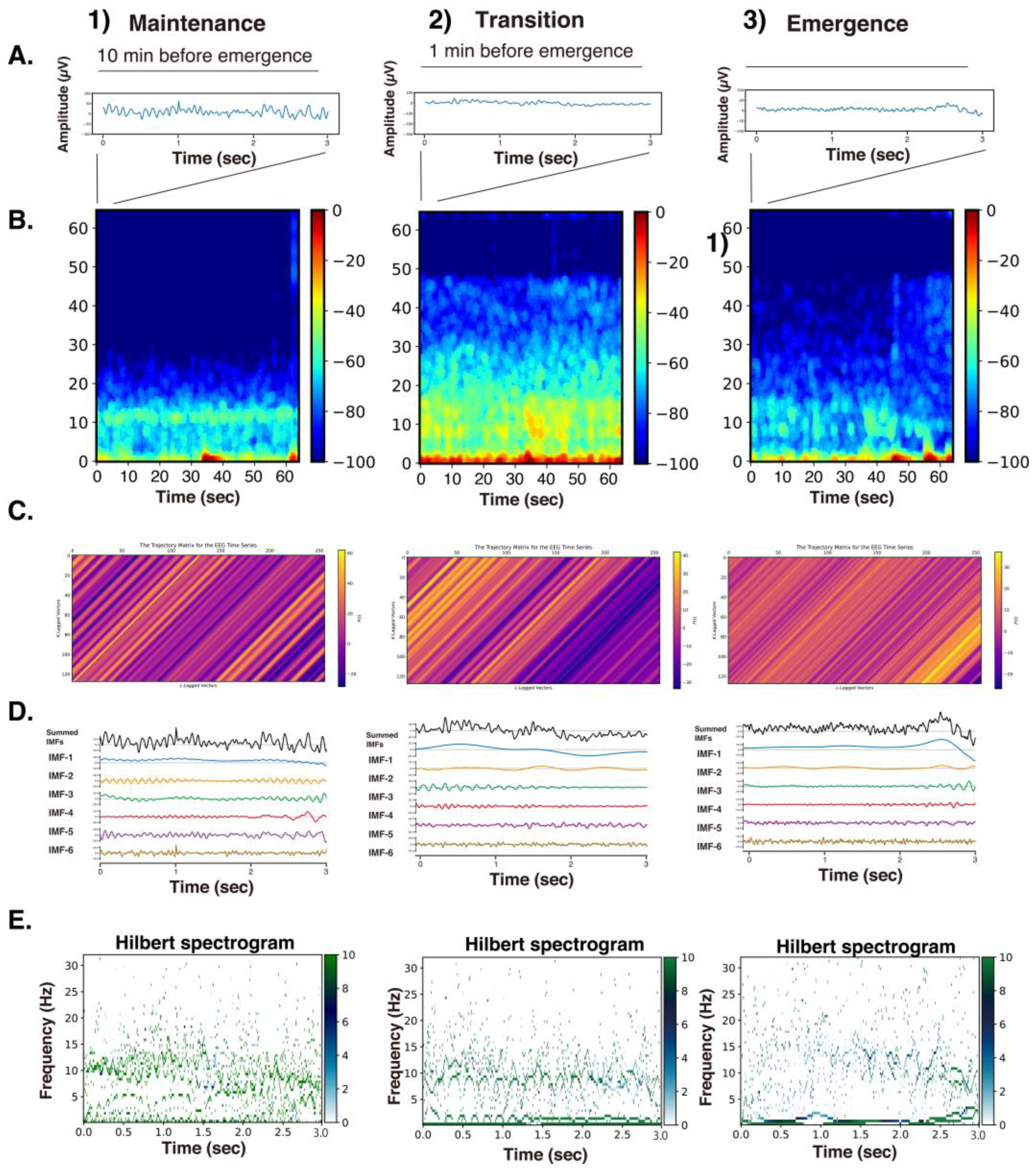
Figure 3 presents the raw EEG data (3 s), density spectral arrays (DSAs) (64 s, starting with a 3 s long segment of raw EEG data), trajectory matrix images of EEG time series, IMFs obtained over 3 s via the SSA method, and Hilbert spectrograms across these GA phases for Patient #1 (54-year-old woman, Yamada et al., 2023 [2]). During the maintenance phase of anesthesia, IMFs 1-4 were predominantly in the frequency range of around 15 Hz or lower. In the DSA during the maintenance phase, an enhancement of α waves characteristic of sevoflurane general anesthesia was observed, with increased power around 12 Hz. Correspondingly, spindle waves, indicative of α wave enhancement, were visible in the EEG waveform. In the DSA during the transitional phase, while the α enhancement persisted, there was an additional increase in higher-frequency components between 15 and 47 Hz. Compared to that for the maintenance phase, the EEG waveform showed reduced amplitude and the emergence of fast-frequency components.

In the awakening phase, the α wave enhancement disappeared, and although the fast-frequency components persisted, an overall reduction in power was observed. The EEG waveform during this phase was predominantly composed of low-amplitude β wave activity. When the trajectory matrices were compared across the three phases, the maintenance and transitional phases exhibited coarser diagonal striations indicative of periodicity, whereas the awakening phase showed finer diagonal patterns. The middle panels of Figure 3 display the six IMFs of the EEG signals, obtained through SAA. In the maintenance phase, IMF-2 and IMF-3 captured the spindle waves associated with enhanced α activity. In the transitional phase, the spindle wave in IMF-2 disappeared. In the awakening phase, IMF-1 through IMF-3 presented nearly flat waveforms, while IMF-5 and IMF-6 predominantly exhibited fast wave activity. The bottom panels of Figure 3 show the Hilbert spectrograms for each IMF over a 3-second interval, depicting the time series relationship between IA and IF obtained via Hilbert transform. In the maintenance phase, a characteristic band around 10 Hz was evident. This feature was also present around 8–10 Hz during the transitional phase. However, in the awakening phase, these characteristic bands disappeared.

3.2. Hilbert Spectrograms of the IMFs in the SSA Method

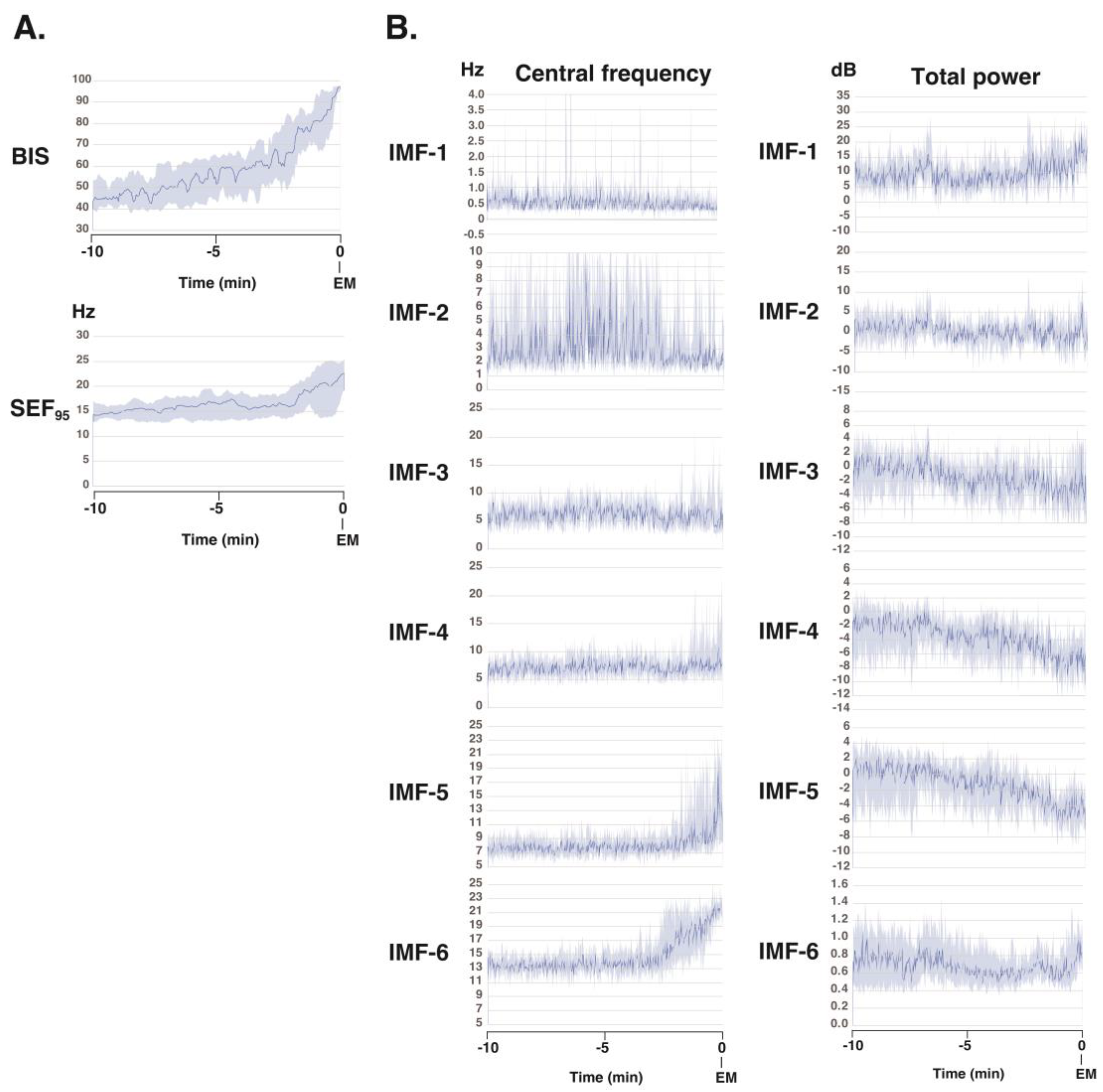
To gain further understanding of the frequency characteristics of each IMF produced via SSA across the 10-minute phase before emergence, a Hilbert spectral analysis of the IMFs was performed. This analysis assessed variations in the IF and IA values derived from the Hilbert transforms of the IMFs across each phase for all 10 patients (Figure 4). Video images (Additional files 4-13) present the analysis screens (the Hilbert spectrograms for each IMF obtained via the SSA method, the summed IMF (IMF-all, which corresponds to the original EEG data), and the DSAs for 30 min until emergence) for the 30-minute period up to the awakening phase in these 10 cases. During the 10-minute period from the maintenance phase of general anesthesia to the awakening phase, the BIS value gradually increased from approximately 45 to 95. The SEF₉₅ began to rise two minutes prior to awakening, increasing from around 14 Hz to approximately 23 Hz at the time of awakening. Using SAA, the EEG was decomposed into six IMFs, and the changes in IF for each IMF were analyzed. IMF-1 showed a mild, gradual decrease; IMF-2 exhibited significant variability; IMF-3 and -4 remained relatively stable; IMF-5 began to increase two minutes before awakening; and IMF-6 began to increase three minutes before awakening. Regarding the changes in IA of each IMF, IMF-1 showed a mild, gradual increase, while IMF-2 through -5 demonstrated a gradual decrease.

3.4. Multiple Linear Regression Models to Predict the BIS

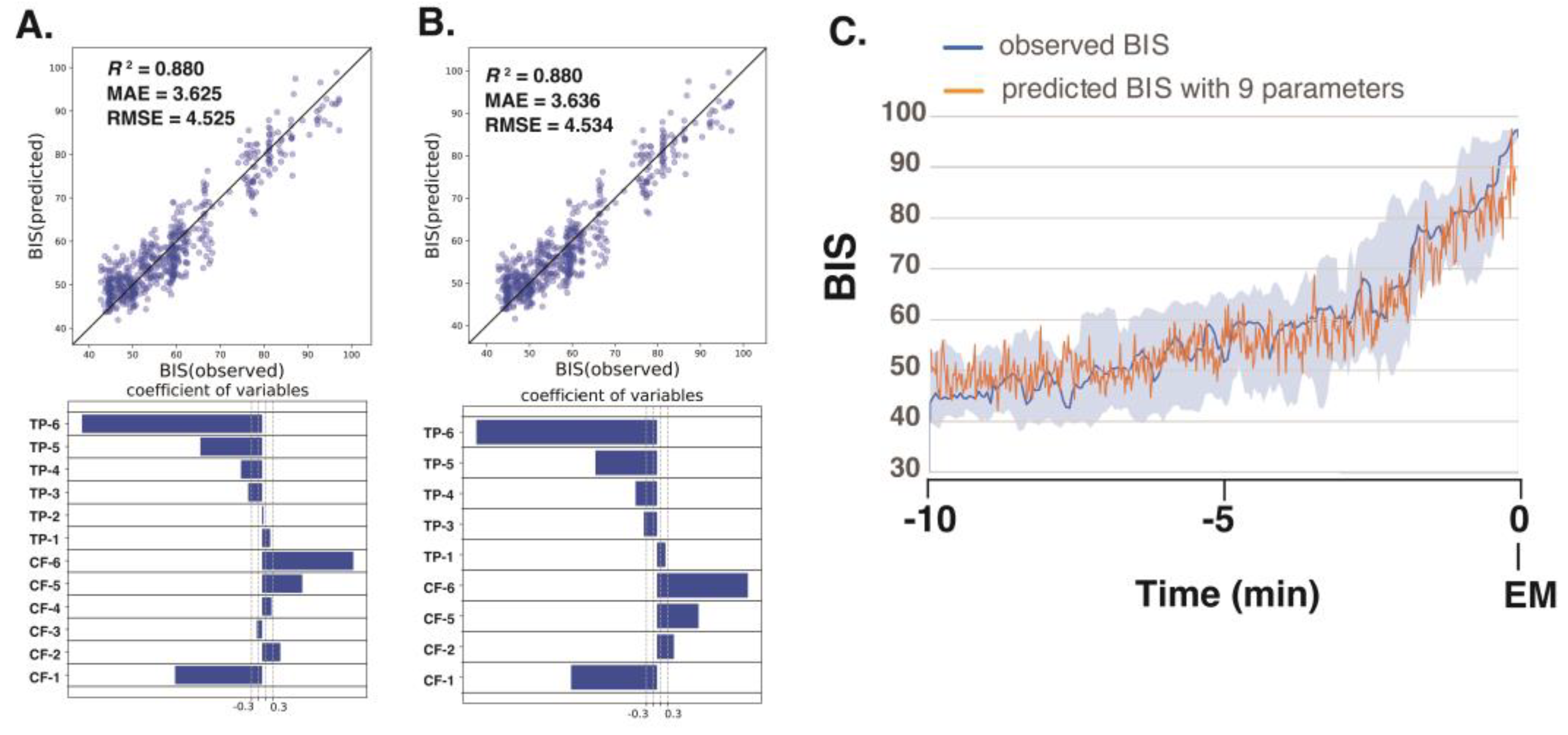
Next, we analyzed the processed EEG data, sampled every 8 s, acquired 10 min before emergence from 10 patients who had been administered sevoflurane GA. We explored the relationship between the BIS (a clinical gauge of the depth of anesthesia) and the IMF parameters, including the center frequency (i.e., the average of the Hilbert spectrum) and TP, which were converted from power in P(µV²) to decibels (dB) using dB = 10 · log10P. Multiple linear regression (MLR) models were developed using IMF parameters to predict the BIS using the Data_EME10s dataset. The comprehensive MLR formula included individual terms for the center frequencies and the TPs of the six IMFs, yielding a model with 12 explanatory variables.

The analysis yielded robust correlations, with the SSA-based MLR model using all 12 parameters (6 center frequencies and 6 TPs) demonstrating the strongest correlation (R²=0.880) and the lowest errors (mean absolute error: MAE = 3.625; root-mean-squared error: RMSE = 4.525) among the four models examined; the results are detailed in Table 1. Notably, in the SAA approach, the center frequencies of IMF-1, IMF-2, IMF-5, and IMF-6 and the TPs of IMF-1, IMF-3, IMF-4, IMF-5, and IMF-6 were identified as significant predictors. For a more targeted approach, we evaluated an MLR model using only nine IMF parameters (IMF-1_freq, IMF-2_freq, IMF-5_freq, IMF-6_freq, IMF-1_TP, IMF-3_TP, IMF-4_TP, IMF-5_TP, and IMF-6_TP) that presented significant p-values (less than 0.05), and the model still presented excellent fit metrics (R²=0.880, MAE = 3.636, RMSE = 04.534) (Figure 5). This finding indicates that SAA effectively captures narrow-band changes in IMF parameters correlated with shifts in the BIS during emergence from GA, thereby demonstrating superior sensitivity for monitoring changes in the depth of anesthesia. The multiple linear regression equation derived from these nine significant parameters was used to predict BIS values over the 10-minute period leading up to awakening, and the predicted values accurately reflected the actual changes in the measured BIS values.

4. Discussion

Monitoring the depth of general anesthesia using EEG remains a complex challenge, largely due to variability in anesthetic agents and patient-specific factors such as age-related neurophysiological differences in pediatric and geriatric populations. Although EEG-based depth indices provided by commercially available monitors have proven useful [7] [9], they are primarily calibrated for intravenous agents like propofol and volatile anesthetics such as sevoflurane. This narrow optimization limits their generalizability to other anesthetic agents and patient groups. To improve depth-of-anesthesia monitoring, a more robust approach grounded in physiologically informed, scientifically validated algorithms is needed.

Quantitative analysis of these EEG spectral dynamics is essential for developing mathematical models that accurately capture the relationship between anesthetic pharmacodynamics and the depth of anesthesia. Such models could substantially enhance the precision and universality of depth-of-anesthesia assessments across diverse clinical scenarios. Frontal EEG signals recorded during GA exhibit characteristic changes in response to anesthetic-induced modulation of neurophysiological activity. Specifically, there is a marked suppression of higher-frequency β and γ activity—typically associated with alertness—while the power of slower-frequency components, such as δ and θ waves, increases, reflecting deeper hypnotic states [4,5,6]. Additionally, a pronounced rise in α activity, often associated with sleep spindles, is observed as anesthesia deepens.

To more effectively extract such EEG features, our recent study examined the use of mode decomposition techniques—EMD, VMD, and EWT—combined with the Hilbert transform, which offers a higher temporal resolution than conventional Fourier-based approaches [2,14]. While both VMD and EWT effectively capture frequency dynamics, they exhibit inconsistencies in assigning narrow-band components across successive epochs, limiting their reliability for continuous depth-of-anesthesia assessment. On the other hand, wavelet mode decomposition (WMD), which we previously reported as an application of EWT, can stabilize the central frequency and TP of the IMFs by using predefined frequency bands [14]. This method demonstrated a strong correlation with BIS values, particularly during the critical 10-minute period from maintenance to emergence from anesthesia. Multiple regression analysis revealed that specific central frequencies and TP values of WMD-derived IMFs were significantly associated with changes in the depth of anesthesia. However, decomposing EEG signals into fixed frequency bands is conceptually equivalent to applying bandpass filters. Although this strategy is useful when the frequency bands of interest are well defined, it carries the inherent risk of missing characteristic changes that span multiple frequency bands, particularly when the relevant spectral features are not clearly established.

To address these limitations, we applied SSA for the first time to extract frequency features from EEG signals recorded during general anesthesia. EEG signals under general anesthesia exhibit time-varying, nonlinear, and non-stationary characteristics. SSA enables the decomposition of such complex signals while preserving their intrinsic statistical structure [25]. Unlike linear approaches such as the Fourier transform, SSA provides high-fidelity separation of trends, periodic components, and noise, making it a promising method for characterizing EEG dynamics under anesthesia. The elementary components derived from SSA capture distinct rhythmic activities such as α (8–13 Hz) and θ (4–7 Hz) waves, which are modulated by anesthetic agents. These components change in proportion to the depth of anesthesia and can be used to extract quantitative, phase-preserving indicators of anesthetic depth. Trajectory matrices and singular vectors obtained via SSA effectively visualize and quantify dynamic changes in EEG across the different anesthetic phases—maintenance, transition, and emergence. This approach offers potential as a real-time analytic framework for assessing state transitions under general anesthesia. EEG decomposition via SSA, when integrated with deep learning and state-space modeling, holds promise for advancing precision anesthesia—individualized anesthetic management tailored to patient-specific neurophysiological responses. Such innovations may enhance patient safety and reduce the risk of over-anesthesia.

In contrast to the Fourier transform, which decomposes signals into frequency components to generate spectrograms, the combined application of mode decomposition and the Hilbert transform offers a more refined approach to feature extraction. This method enables the calculation of the IF and IA at each data point, producing high-resolution spectrograms that more accurately reflect the signal’s dynamic characteristics. By comparison, Fourier-based power spectral analysis—for instance, using 0.25 Hz frequency bins for a 128 Hz EEG sampling rate—requires at least 512 data points (equivalent to 4 seconds of EEG) and only achieves a temporal resolution of 2 seconds under a 50% window overlap. In this context, decomposing EEG signals into narrow-band intrinsic mode functions (IMFs) significantly improves the temporal resolution and enhances the granularity of time–frequency representations. The resulting Hilbert spectrogram allows for more detailed and precise analysis of non-stationary EEG signals.

The limitations of this study are inherently linked to a fundamental and unresolved question: What precisely constitutes the depth of anesthesia? [26] Currently, commercially available monitors rely on indices such as the BIS and patient state index (PSi) as surrogate markers for anesthetic depth. However, the proprietary nature of the algorithms underlying these indices renders their validity difficult to verify through direct comparison. In this study, we examined the relationship between BIS values and parameters derived from the Hilbert spectra of IMFs obtained via mode decomposition. Although the algorithm used to calculate the BIS has not been fully disclosed, this study demonstrated the potential for capturing changes in the frequency components of EEG signals during general anesthesia using singular spectrum analysis, a linear-algebra-based approach, and to translate these findings into a technique for assessing the depth of anesthesia.

5. Conclusions

This study demonstrated that SSA combined with the Hilbert transform enables high-resolution, physiologically meaningful decomposition of EEG signals from patients under general anesthesia. SSA effectively extracted time-varying features associated with anesthetic depth transitions, offering superior temporal precision. Multiple regression models using SSA-derived features accurately predicted BIS values, highlighting SSA’s potential for improving real-time anesthesia monitoring.

References

- Yamada, T.; Obata, Y.; Sudo, K.; Kinoshita, M.; Naito, Y.; Sawa, T. Changes in EEG frequency characteristics during sevoflurane general anesthesia: feature extraction by variational mode decomposition. J Clin Monit Comput 2023, 37, 1179–92. [Google Scholar] [CrossRef]
- Obata, Y.; Yamada, T.; Akiyama, K.; Sawa, T. Time-trend analysis of the center frequency of the intrinsic mode function from the Hilbert-Huang transform of electroencephalography during general anesthesia: a retrospective observational study. BMC Anesthesiol 2023, 23, 125. [Google Scholar] [CrossRef]
- Purdon, P. L.; Sampson, A.; Pavone, K. J.; Brown, E. N. Clinical electroencephalography for anesthesiologists: part I: background and basic signatures. Anesthesiology 2015, 123, 937–60. [Google Scholar] [CrossRef]
- Supp, G. G.; Siegel, M.; Hipp, J. F.; Engel, A. K. Cortical hypersynchrony predicts breakdown of sensory processing during loss of consciousness. Curr Biol 2011, 21, 1988–93. [Google Scholar] [CrossRef] [PubMed]
- Ching, S.; Cimenser, A.; Purdon, P. L.; Brown, E. N.; Kopell, N. J. Thalamocortical model for a propofol-induced alpha-rhythm associated with loss of consciousness. Proc Natl Acad Sci U S A 2010, 107, 22665–70. [Google Scholar] [CrossRef]
- Flores, F. J.; Hartnack, K. E.; Fath, A. B.; Kim, S. E.; Wilson, M. A.; Brown, E. N.; Purdon, P. L. Thalamocortical synchronization during induction and emergence from propofol-induced unconsciousness. Proc Natl Acad Sci U S A 2017, 114, E6660–E6668. [Google Scholar] [CrossRef] [PubMed]
- Roche, D.; Mahon, P. Depth of Anesthesia Monitoring. Anesthesiol Clin 2021, 39, 477–492. [Google Scholar] [CrossRef] [PubMed]
- Brook, K.; Agarwala, A. V.; Li, F.; Purdon, P. L. Depth of anesthesia monitoring: an argument for its use for patient safety. Curr Opin Anaesthesiol 2024, 37, 689–696. [Google Scholar] [CrossRef]
- Brook, K.; Ferraton, M.; Dreher, L.; Lambert, D. H.; Feldman, J. M.; Connor, C. W. Electroencephalographic Depth-of-Anesthesia Monitoring. A A Pract 2025, 19, e01895. [Google Scholar] [CrossRef]
- Nguyen-Ky, T.; Wen, P.; Li, Y.; Malan, M. Measuring the hypnotic depth of anaesthesia based on the EEG signal using combined wavelet transform, eigenvector and normalisation techniques. Comput Biol Med 2012, 42, 680–91. [Google Scholar] [CrossRef]
- Huang, N. E.; Shen, Z.; Long, S. R.; Wu, M. C.; Shih, H. H.; Zheng, Q.; Yen, N.-C.; Tung, C. C.; Liu, H. H. The empirical mode decomposition and the Hilbert spectrum for nonlinear and non-stationary time series analysis. Proceedings: Mathematical, Physical and Engineering Sciences 1998, 454, 903–5. [Google Scholar] [CrossRef]
- Dragomiretskiy, K.; Zosso, D. Variational mode decomposition. IEEE Transactions on Signal Processing 2014, 62, 531–4. [Google Scholar] [CrossRef]
- Gilles, J. Empirical wavelet transform. IEEE Trans Signal Process 2013, 61, 3999–4010. [Google Scholar] [CrossRef]
- Yamochi, S.; Yamada, T.; Obata, Y.; Sudo, K.; Kinoshita, M.; Akiyama, K.; Sawa, T. Wavelet transform-based mode decomposition for EEG signals under general anesthesia. PeerJ 2024, 12, e18518. [Google Scholar] [CrossRef]
- D'ARCY, J. Introducing SSA for Time Series Decomposition. https://www.kaggle.com/code/jdarcy/introducing-ssa-for-time-series-decomposition (Dec 12, 2025).
- Singular spectrum analysis. https://en.wikipedia.org/wiki/Singular_spectrum_analysis (Dec 12, 2025).
- scikit-learn. Machine Learning in Python. https://scikit-learn.org/stable/ (Dec 13, 20205).
- Kortelainen, J.; Vayrynen, E. Assessing EEG slow wave activity during anesthesia using Hilbert-Huang Transform. Annu Int Conf IEEE Eng Med Biol Soc 2015, 2015, 117–20. [Google Scholar]
- Liu, Q.; Ma, L.; Fan, S. Z.; Abbod, M. F.; Ai, Q.; Chen, K.; Shieh, J. S. Frontal EEG temporal and spectral dynamics similarity analysis between propofol and desflurane induced anesthesia using Hilbert-Huang transform. Biomed Res Int 2018, 2018, 4939480. [Google Scholar] [CrossRef] [PubMed]
- Li, X.; Li, D.; Liang, Z.; Voss, L. J.; Sleigh, J. W. Analysis of depth of anesthesia with Hilbert-Huang spectral entropy. Clin Neurophysiol 2008, 119, 2465–75. [Google Scholar] [CrossRef]
- Shalbaf, R.; Behnam, H.; Sleigh, J. W.; Voss, L. J. Using the Hilbert-Huang transform to measure the electroencephalographic effect of propofol. Physiol Meas 2012, 33, 271–85. [Google Scholar] [CrossRef]
- Hayase, K.; Kainuma, A.; Akiyama, K.; Kinoshita, M.; Shibasaki, M.; Sawa, T. Poincare plot area of gamma-band EEG as a measure of emergence from inhalational general anesthesia. Front Physiol 2021, 12, 627088. [Google Scholar] [CrossRef]
- Statsmodels. https://www.statsmodels.org/stable/index.html (Dec 13, 2025).
- Sawa, T.; Yamada, T.; Obata, Y. Power spectrum and spectrogram of EEG analysis during general anesthesia: Python-based computer programming analysis. J Clin Monit Comput 2022, 36, 609–1. [Google Scholar] [CrossRef] [PubMed]
- Hassani, H. A Brief Introduction to Singular Spectrum Analysis. https://ssa.cf.ac.uk/ssa2010/a_brief_introduction_to_ssa.pdf (Dec 13, 2025).
- Sleigh, J. W. Depth of anesthesia: perhaps the patient isn't a submarine. Anesthesiology 2011, 115, 1149–50. [Google Scholar] [CrossRef] [PubMed]