
Submitted:
08 July 2025
Posted:
09 July 2025
You are already at the latest version
Abstract
Background/Objectives: Autism Spectrum Disorder (ASD) diagnosis is challenging due to the complexity of Electroencephalogram (EEG) signals. This study aims to enhance the accuracy of ASD diagnosis by combining Fisher Linear Discriminant Analysis (FLDA) and Stationary Wavelet Transform (SWT) for effective classification of EEG signals. Methods: EEG signals were filtered and decomposed into frequency bands using SWT. Level 3 (gamma), level 4 (beta), and level 6 (theta) components were extracted. FLDA was used to lower dimensionality and enhance class separation between ASD and normal EEG. Classification accuracy was evaluated using a confusion matrix. Results: The combined approach of FLDA and SWT achieved a classification accuracy exceeding 90%, with 96% accuracy in classifying level 6 (theta) components in the normal class, demonstrating the method's potential to enhance early detection of ASD. Conclusions: Integrating FLDA and SWT in EEG analysis offers a novel and effective approach to enhancing ASD diagnosis accuracy and efficiency. The method offers a reliable tool for supporting early ASD diagnosis in clinical settings.
Keywords:
autism spectrum disorder (ASD)
; electroencephalogram (EEG)
; fisher linear discriminant analysis (FLDA)
; stationary wavelet transform (SWT)
; confusion matrix
1. Introduction
The Neurodevelopmental Autism Spectrum Disorder (ASD) is a complex cranial nerve disorder that significantly impacts the growth and behavioral development of affected children [1]. This syndrome is characterized by repetitive behavioral patterns [2]. Based on research, many children with autism remain undiagnosed or do not receive appropriate treatment, largely due to environmental factors and the inadequacy of diagnostic equipment [3]. With advances in technology, especially in the use of an electroencephalogram (EEG) [4,5], detecting autism in children is potentially becoming easier. This can be achieved by recording brain signals via a Brain-Computer Interface (BCI) with a collection of electrodes placed on the scalp [6]. However, with complex EEG signals, this research requires a Machine Learning (ML) scheme to analyze signal patterns that are difficult to analyze. ML technique effectively utilizes real-time processing methods for EEG signals [7]. Automation of the detection method reduces reliance on manual inspection by highly specialized experts, leading to quicker responses and potentially enhancing the overall outcomes of classification management [8].
The integration of ML in biomedical fields is not only revolutionizing diagnostics but also optimizing operations across various industries, including manufacturing, where it has proven effective in cost estimation [9] (Ma'ruf et al., 2024). The potential of ML to enhance the accuracy of autism predictions is significant, potentially saving time and resources in clinical settings [10].
Recent studies have demonstrated the effectiveness of ML in detecting brain abnormalities through EEG. For instance, Grossi et al. established a predictive model differentiating between autism and neurotypical development, achieving an accuracy of 93.2% using the k-Nearest Neighbor (kNN) algorithm [11]. Further advancements by Aljalal et al. employed Variational Mode Decomposition (VMD) in conjunction with k-Nearest Neighbors (kNN) to detect Mild Cognitive Impairment (MCI), achieving a remarkable accuracy of 99.81% [12]. Similarly, Al-Jumaili et al. demonstrated the utility of various ML algorithms with feature extraction methods for detecting epileptic seizures, obtaining an accuracy of 96% with Support Vector Machine (SVM) [13]. In the context of autism detection, Melinda et al. utilized SVM combined with Continuous Wavelet Transform (CWT) to achieve a 95% classification accuracy for autistic children [14]. Chaddad et al. provided a comprehensive analysis of various EEG signal classification techniques, underscoring the potential of ML algorithms to achieve high accuracy [15].
Among the various ML methods, Fisher Linear Discriminant Analysis (FLDA) is particularly notable for its application in statistics and pattern recognition. This technique effectively classifies data while maximizing class separation, making it an ideal choice for our study [16,17]. This method was chosen because it can produce good accuracy and improve system performance [18,19]. FLDA is a supervised learning technique that is used to reduce dimensions while classifying data by maximizing the distance between classes [20]. This method will be combined with the Stationary Wavelet Transform (SWT) method to filter and extract signals at certain frequencies. This research builds upon a previous journal article that utilized the Discrete Wavelet Transform (DWT) extraction and Linear Discriminant Analysis (LDA) in processing EEG data from individuals with autism and those without [18]. The difference lies in the component extraction method used, which utilizes only one detailed component, represented by a beta signal. The results of this follow-up research include the classification of three-component extractions and the accuracy of implementing FLDA on autistic and normal EEG signals.
Stationary Wavelet Transform (SWT) is a digital signal processing technique that simultaneously filters and extracts signals to certain frequencies through Low-Pass Filter (LPF) and High-Pass Filter (HPF) processes [21]. SWT extraction will produce three attributes in the form of levels 3, 4, and 6 components, which are gamma, beta, and theta signals, respectively. This component is a feature chosen to test the performance of the FLDA system in classifying signals. The use of this wavelet technique can also help increase noise suppression in EEG signals through denoising techniques [15]. The advantage of using the SWT technique is that it does not require down-sampling or up-sampling. In this case, the number of coefficients and diffusion levels remains constant, or the length of the transformation signal at each level is fixed [22].
The objective of this study is to develop a robust classification system for EEG signals from autistic and typically developing children by combining FLDA with SWT. This approach aims to enhance signal extraction and noise suppression, thereby facilitating more accurate classification of ASD and typical EEG data. The study's major contributions can be summarized as follows. This research presents a novel approach that integrates Fisher Linear Discriminant Analysis (FLDA) with the Stationary Wavelet Transform (SWT) for classifying EEG signals from autistic and normal children. The study offers an in-depth evaluation of the system's performance based on confusion matrix metrics, including accuracy, precision, recall, and F1-score. A comparative analysis of FLDA's effectiveness in classifying multiple EEG components (gamma, beta, and theta signals) extracted through SWT highlights the method's versatility.
The research aims to enhance clinical diagnostics and improve early intervention strategies for children with autism by providing a reliable and automated detection method for ASD through EEG analysis.
2. Materials and Methods
This study applies the SWT and FLDA methods to process the data (see Figure 1). SWT is used to denoise signals and extract signals into several different frequencies. The results of SWT extraction will be presented in the form of three frequency attributes, corresponding to levels 3, 4, and 6 components, which represent gamma, beta, and theta signals, respectively. The denoising or noise suppression process in SWT utilizes the thresholding feature. The three levels of filtering and decomposition results will later be used as features for FLDA classification testing. Meanwhile, FLDA is used to classify signals in autistic and normal syndromes. This research aims to compare the accuracy results of EEG classification for autistic and normal individuals using the FLDA technique, based on head condition in terms of frequencies at each level.
2.1. Datasets
This study used an EEG dataset provided by King Abdulaziz University (KAU), Jeddah, Saudi Arabia [23]. This dataset comprises 16 EEG signals, including 8 EEG samples from autistic children and 8 EEG samples from typically developing children, recorded using the BCI2000 viewer in a .dat format with a 16 x 16 (trial x channel) resolution and a frequency of 100 Hz. Each sample contains 16 channels consisting of FP1, F3, F7, T3, T5, O1, C4, FP2, FZ, F4, F8, C3, CZ, PZ, OZ, and O2. The dataset ensures the confidentiality of all participants by excluding any personal identification information. The recorded EEG signals represent a diverse demographic, including eight subjects with ASD (5 males and 3 females, aged 6 to 20 years) and eight control subjects (all males, aged 9 to 13 years). This inclusion of a range of ages and both genders among the ASD participants increases the validity and generalizability of the research findings. The EEG recordings were captured using Ag/AgCl electrodes in conjunction with a g.tec EEG device and a g.tec USB amplifier while the subjects were in a relaxed state. For researchers interested in accessing this dataset, inquiries can be directed to Dr. Mohammed Jaffer Alhaddad via email at malhaddad@kau.edu.sa.
2.2. Data Input Preprocessing
In this section, EEG datasets were input with a frequency of 256 Hz. At the data import stage, the function type used is BCI2000. This is because the EEG signal recording format has an output in ".dat" format. Then, to obtain information from the signal, import event information from each recorded channel, namely 16 events per data sample. This process produces a data length of 16,000 for 16 EEG samples, with each sample cut every 4 seconds. Then, the data is exported in double (number) form to produce a signal output in .txt data format.
2.3. Stationary Wavelet Transform (SWT)
Feature extraction and selection techniques significantly contribute to improving BCI capabilities across various applications, including cognitive enhancement and neuroprosthetics [24]. This research utilizes SWT to decompose and filter signals into smaller dimensions through the Low-Pass Filter (LPF) process, which filters low-frequency signals, and the High-Pass Filter (HPF) process, which filters high-frequency signals. SWT is a modified method of the Discrete Wavelet Transform (DWT), also known as Undecimate Wavelet Transform. SWT does not have down-sampling or up-sampling, so the number of coefficients and decomposition levels remains constant at each level, resulting in faster computation. The filtering process produces subsample results as described in the formula [25].
where is the mother wavelet, a is a scale parameter, b is a shift parameter, and ψ*(t) is the complex conjugate of the mother wavelet. The discrete values and shift parameters are a = 2j and b = 2j k.
SWT utilizes a thresholding function to remove noise by setting small-amplitude wavelet coefficients (representing noise) to zero or a specified threshold value [26]. The choice of threshold value must be optimal. A threshold value that is too small can leave noise, while one that is too large can erase valid signal information. Therefore, selecting an optimal threshold value is crucial to minimize the Mean Squared Error (MSE) [27]. There are two basic wavelet Shrinkage functions, namely, hard threshold and soft threshold [28].
2.4. Hard Threshold
A hard threshold is a linear function that removes coefficients below a threshold value determined by the noise variance. The hard threshold filter coefficient is obtained from:
This wavelet is known as a "keep or kill" procedure. Thresholding is better known because the thresholding function has a discontinuity; therefore, x values above the lambda threshold are not affected. Conversely, if they are below the lambda threshold, they will be changed to 0.
2.5. Soft Threshold
The soft thresholding function is typically used because it remains continuous, ensuring that x values above the λ threshold are included in the estimation process. The soft threshold filter can be stated as follows:
where is the signal to be analyzed, λ is a threshold parameter, and x is a discrete parameter. The primary difference between the hard and soft threshold functions is that the coefficient below the threshold is set to zero in the hard threshold. Thus, this will weaken the signal oscillations, and the reconstructed signal will have poor smoothness [29]. Based on the graph, the signal created will follow the shape of the original signal; however, if the coefficient is less than or equal to the threshold value, it will be set to zero, which can compromise the interpretation of the data. Meanwhile, with soft thresholding, the graph created will follow the shape of the signal without destroying the data. The following is an SWT chart for decomposing and extracting signals into smaller frequencies.
Based on Figure 2, the EEG signal will be extracted, decomposed, and filtered into 6 levels through a High-Pass Filter (detail component) and Low-Pass Filter (approximation component) process. The mother wavelet filter used is Daubechies type 4 (Db-4). This wavelet has proven to be very suitable for processing raw EEG signals and has been proven to produce the best signal filtering [30]. Next, these three detailed components are utilized, which are produced in the form of signals at levels 3, 4, and 6, corresponding to gamma, beta, and theta signals, respectively. These three levels were chosen because they can represent the conditions of autistic and normal children when they are sleeping, active, and focused.
The denoising process is carried out by utilizing threshold and sampling functions through the Low-Pass Filter and High-Pass Filter processes. This type of soft thresholding was chosen to eliminate noise because it can smooth the reconstructed signal without distorting it, thereby preserving the signal integrity [21]. Therefore, the resulting signal graph will retain the same information as the original signal graph.
2.6. Fisher Linear Discriminant Analysis (FLDA)
Fisher Linear Discriminant Analysis (FLDA) is an efficient method for disaggregating data and making predictions, reducing the risk of overfitting and excessive computation. FLDA focuses on maximizing the distance between classes while minimizing the distance within classes (Sw) and maximizing the distance between classes (Sb). This method is included in ML by using labeled data to predict new data labels [31]. FLDA uses the hyperplane function to differentiate data from various classes [32,33,34]. A hyperplane is a function that allows data classification based on distinguishing features between classes. The classification steps using FLDA are as follows [34,35]:
Convert a two-dimensional matrix to one dimension by converting it into row or column vector form.
The training data obtained is then grouped into a matrix of several classes ().
Calculate the mean for each class () based on the orientation of the training data vector: row or column, according to the vector used. The mean number of dimensions will be the same as the dimensions of one training data point, not the entire dataset.
is the number of class samples of the i-th, is the average vector of the i-th class, and x is the class sample.
Calculate the total mean value of all classes () with the following equation:
is a sample in class of the i-th, and It is a sample in class C.
Calculating the between-class scatter matrix (Sb) and the within-class scatter matrix (Sw).
Sb is the spread matrix between classes, and Sw is the spread. Matrix in the class, is the total number of classes, sample in the j-th class, is a vector of means of the number of samples, and is the transpose function.
Calculate the covariance matrix value () by using the value of (Sb) and (Sw) as follows:
where is the covariance matrix.
Calculate eigenvalues () and eigenvectors () with the following equation:
where is an eigenvalue function, and is an eigenvector function.
Choose eigenvectors with eigenvalue , and express them with a matrix .
Calculate the data projection with the selected eigenvector using the equation:
is a function, and the projection is vector eigen transpose, and It is a scatter.
As shown in Figure 3, the data is divided into training data (70%) and testing data (30%) for FLDA performance testing. Predictions on testing data use a model trained with input in the form of SWT extraction results. FLDA's effectiveness is measured using the Confusion Matrix, which provides metrics such as Accuracy, Precision, Recall, and F1-Score.
3. Results
There are discussion results from the methods used by SWT and FLDA to classify autistic and normal EEG by producing the best accuracy.
3.1. Data Input Preprocessing Results
In processing normal and autistic EEG data, only 15 of the 16 active channels were read, namely FP1, F3, F7, T3, T5, O1, C4, FP2, FZ, F4, F8, C3, CZ, PZ, and OZ. Channel O2 is not read because it is considered a grounding channel. The input process involved 16 iterations for 16 patients with 15 channels, a total of 240,000 features. The dataset comprises 16,000 data points, divided into 8,000 normal EEG data points and 8,000 autistic EEG data points. Labels on EEG channels indicate electrode positions on the head, such as F (Frontal), Fp (Frontopolar), C (Central), O (Occipital), and T (Temporal).
3.2. Stationary Wavelet Transform (SWT) Result
In this study, SWT is used to extract and filter signals to certain frequencies using Daubechies 4 (db-4) as the mother wavelet. Extraction yields three detailed components, namely levels 3, 4, and 6, which represent the gamma signal, beta, and theta, respectively. The results obtained from feature extraction and denoising for the normal and ASD classes are presented in Table 1, Table 2, Table 3, Table 4, Table 5 and Table 6 below.
The results of the SWT data in the frequency range of 32–64 Hz (level 3) indicate that the patient's brain activity is in a focused state (Table 1 and Table 4). The frequency range of 16–32 Hz (level 4) shows normal brain activity (Table 2 and Table 5). The frequency range of 4–8 Hz (level 6) shows brain activity in sleep (Table 3 and Table 6). From the results obtained, the normal EEG is predominantly higher and more stable compared to the autistic EEG. The electrical activity of normal children experiences greater fluctuations, meaning that the channels in the normal EEG are more active. Meanwhile, frequency fluctuations produced by autistic children experience inconsistent up-and-down changes and tend to be smaller. These conditions can affect the accuracy of FLDA classification performance.
3.3. Fisher Linear Discriminant Analysis (FLDA) Result
FLDA's primary goal is to effectively separate different features by transforming data into a lower-dimensional space, maximizing the distance between classes, and minimizing the distance within the same classes. FLDA takes normal and autistic EEG datasets, each of which has 15 active channel parameters, and converts them into one representative value. FLDA creates new axes based on data characteristics, which reduces variance and maximizes the distance between classes. The results of normal and autistic EEG classification show good separation based on each feature, as shown in Figure 4
Figure 4 visualizes the results of normal and autistic EEG classification using the FLDA algorithm, with three components: level 3 (red) represents gamma, level 4 (green) represents beta, and level 6 (blue) represents theta. The normal EEG classification results show good separation. At the same time, the autistic EEG data exhibit some overlap due to non-linear data characteristics; however, this does not affect the performance of the FLDA system, as documented in Table 7.
The results of calculating the normal EEG confusion matrix are in Table 7. The length of normal EEG data is 8,000. The TP value is 2,975, the FP value is 119, the FN value is 50, and the TN value is 4,856. The correctly predicted TP is 2,975 data, the incorrectly predicted FP is 119 data, the incorrectly predicted FN is 50 data, and the correctly predicted TN is 4,856 data.
Based on Table 8, Level 3 has a Precision of 96%, a recall of 98%, and an F1-score of 97%. Level 4 has a Precision of 96%, a recall of 94%, and an F1-score of 95%. Level 6 has a Precision of 91%, a recall of 92%, and an F1-score of 91%. The overall accuracy of FLDA classification for normal EEG was 96%, which falls into the excellent category.
Table 9 shows the results of the confusion matrix calculations for autism EEG. The dataset consists of 8,000 data points. The TP value is 1,862, FP is 196, FN is 329, and TN is 5,613. TP that was predicted correctly was 1,862 data, FP that was predicted incorrectly was 196 data, FN that was predicted incorrectly was 329 data, and TN that was predicted incorrectly was 5,613 data.
Lastly, Table 10 shows the results of calculating the confusion matrix parameters for autism EEG. At level 3, precision is 90%, recall is 85%, and F1-Score is 88%. Level 4 obtains a Precision of 94%, a Recall of 96%, and an F1-score of 95%. Meanwhile, level 6 obtained a precision of 73%, a Recall of 78%, and an F1-score of 76%. Overall, the classification accuracy of FLDA on autism EEG was 93%, which is in the very good category.
4. Discussion
This study aims to evaluate the application of the FLDA system in classifying EEG signals from individuals with autism and those without autism, based on accuracy. This classification system separates signals based on detailed components at each level. The results show an accuracy of above 90%, indicating a high level of classification accuracy. FLDA is a suitable choice for ML techniques on autistic and normal EEG signals. However, the accuracy of FLDA on normal EEG is higher than that on autistic EEG, which is caused by the non-linear data characteristics of autistic EEG.
This study also combines the FLDA method, which can reduce dimensions and classify data correctly, with SWT, which is effective in extracting features from EEG signals. This study compared different methods for identifying neurological disorders, especially ASD, alongside previous research. M. N. A. Tawhid et al. proposed a spectrogram and Time-Fourier Transform (STFT) based approach, which achieved an accuracy of 95.25% [36]. Melinda et al. (2023) achieved 99% accuracy using LDA and DWT. F. A. Alturki et al. utilized the Common Spatial Pattern (CSP) and Local Binary Pattern (LBP) methods, achieving 98.46% accuracy [37].
Our study builds on existing research in the field of EEG-based classification, which aims to improve ASD detection. Several recent studies related to this topic have identified advantages and drawbacks, which can be compared with the findings of this study. Compared with previous studies, which focused on various feature extraction methods and classifiers, our approach uses SWT for feature extraction and FLDA for classification. This combination offers several advantages, including effective dimensionality reduction of EEG data and accurate ASD classification. By utilizing SWT, important features can be extracted from EEG signals, thereby enabling a better representation of ASD-related brain activity patterns. However, this approach may have some drawbacks, including the use of relatively small datasets and limited FLDA capabilities. Despite these challenges, this study makes a significant contribution to the classification of ASD EEG signals with competitive accuracy while also emphasizing the efficiency of the simpler FLDA method compared to several other complex techniques used in previous studies. This research supports the development of effective and efficient automated diagnosis systems in the context of neurological disorders such as ASD.
5. Conclusions
This study demonstrates that the combination of SWT and FLDA methods significantly enhances the accuracy of EEG signal processing for both autistic and typically developing subjects, achieving an accuracy rate of over 90%. The key classification parameters include gamma signals (32–64 Hz) at level 3, representing focused brain activity, beta signals (16–32 Hz) at level 4, indicating normal brain activity, and theta signals (4–8 Hz) at level 6, corresponding to brain activity during sleep. These parameters were extracted through SWT using the Daubechies 4 (db-4) mother wavelet, along with soft thresholding for effective filtering. The system demonstrated high accuracy in classifying normal EEG signals at 96%, while the classification accuracy for autistic EEG signals reached 93%, with the slight decrease attributed to overlapping scatter in the data. These results were validated using the confusion matrix method during training and testing. The findings of this research can be applied in practical scenarios, particularly in improving the early detection and classification of autism through EEG analysis.
Additionally, this framework can be extended to more complex brain signal analyses in other neurological disorders [4,5,6,7,8,9,10,11,12,13,14,15,16,17,18,19,20,21,22,23,24,25,26,27,28,29,30,31,32,33,34,35,36,37,38,39,40], with potential wearable applications [41]. However, there are limitations, including the overlap of certain EEG patterns in autistic subjects, which slightly reduces accuracy. Future research could explore more advanced filtering techniques or a larger, more diverse dataset to address this challenge. Further exploration into more sophisticated classification algorithms may also yield higher accuracy and more robust results.
Author Contributions
Conceptualization, F.F. and M.M.; methodology, M.M.; software, F.F.; validation, F.F., M.M. and P.D.P.; formal analysis, F.F. and E.E.; data curation, M.M.; writing—original draft preparation, M.M.; writing—review and editing, F.F. and E.E. ; funding acquisition, F.F., M.M. and P.D.P. All authors have read and agreed to the published version of the manuscript.
Funding
This research was funded by the Ministry of Higher Education, Research and Development of Indonesia, through the RKI 2025 scheme of Universitas Sumatera Utara, Universitas Syiah Kuala, and Universitas Indonesia, grant number 28/UN5.4.10.K/PT.01.03/RKI/2025 dated April 14, 2025.
Institutional Review Board Statement
Not applicable.
Informed Consent Statement
Not applicable.
Data Availability Statement
EEG dataset provided by King Abdulaziz University (KAU), Jeddah, Saudi Arabia. KACST, 8-NAN106-3.
Acknowledgments
None.
Conflicts of Interest
The authors declare no conflicts of interest.
Abbreviations
The following abbreviations are used in this manuscript:
| ASD | Autism Spectrum Disorder |
| EEG | Electroencephalography |
| SWT | Stationary Wavelet Transform |
| FLDA | Fisher Linear Discriminant Analysis |
References
- N. A. Spinazzi, A. B. Velasco, D. J. Wodecki, and L. Patel, “Autism Spectrum Disorder in Down Syndrome: Experiences from Caregivers,” J. Autism Dev. Disord., vol. 54, no. 3, pp. 1171–1180, 2024. [CrossRef]
- M. Derbali, M. Jarrah, and P. Randhawa, “Autism Spectrum Disorder Detection: Video Games based Facial Expression Diagnosis using Deep Learning,” Int. J. Adv. Comput. Sci. Appl., vol. 14, no. 1, pp. 110–119, 2023. [CrossRef]
- J. Zeidan et al., “Global prevalence of autism: A systematic review update,” Autism Res., vol. 15, no. 5, pp. 778–790, 2022. [CrossRef]
- M. Yazid et al., “Simple Detection of Epilepsy from EEG Signal Using Local Binary Pattern Transition Histogram,” IEEE Access, vol. 9, pp. 150252–150267, 2021. [CrossRef]
- S. Firdaus, M. Nasution, and F. Fahmi, “Initial Design For Utilizing Machine Learning In Identifying Diseases In Palm Oil Plant,” Proceeding - ELTICOM 2023 7th Int. Conf. Electr. Telecommun. Comput. Eng. Sustain. Resilient Communities with Smart Technol., pp. 95–99, 2023. [CrossRef]
- A.F. Nurfirdausi, R. A. Apsari, S. K. Wijaya, P. Prajitno, and N. Ibrahim, “Wavelet Decomposition and Feedforward Neural Network for Classification of Acute Ischemic Stroke based on Electroencephalography,” Int. J. Technol., vol. 13, no. 8, pp. 1745–1754, 2022. [CrossRef]
- P. Kumar, S. Chauhan, and L. K. Awasthi, “Artificial Intelligence in Healthcare: Review, Ethics, Trust Challenges & Future Research Directions,” Engineering Applications of Artificial Intelligence, vol. 120. p. 105894, 2023. [CrossRef]
- S. Golla and M. Suman, “Automated Seizure Detection in Neonatal EEG using Signal Processing Algorithms,” J. Adv. Res. Appl. Sci. Eng. Technol., vol. 31, no. 3, pp. 220–227, 2023. [CrossRef]
- Ma’ruf, A. A. R. Nasution, and R. A. C. Leuveano, “Machine Learning Approach for Early Assembly Design Cost Estimation: A Case from Make-to-Order Manufacturing Industry,” Int. J. Technol., vol. 15, no. 4, pp. 1037–1047, 2024. [CrossRef]
- M. S. Farooq, R. Tehseen, M. Sabir, and Z. Atal, “Detection of autism spectrum disorder (ASD) in children and adults using machine learning,” Sci. Rep., vol. 13, no. 1, pp. 1–13, 2023. [CrossRef]
- E. Grossi, R. White, and R. J. Swatzyna, “A Simple Preprocessing Method Enhances Machine Learning Application to EEG Data for Differential Diagnosis of Autism,” Qeios, pp. 1–15, 2024. [CrossRef]
- M. Aljalal, M. Molinas, S. A. Aldosari, K. AlSharabi, A. M. Abdurraqeeb, and F. A. Alturki, “Mild cognitive impairment detection with optimally selected EEG channels based on variational mode decomposition and supervised machine learning,” Biomed. Signal Process. Control, vol. 87, p. 105462, 2024. [CrossRef]
- S. Al-Jumaili, A. D. Duru, A. A. Ibrahim, and O. N. Uçan, “Investigation of Epileptic Seizure Signatures Classification in EEG Using Supervised Machine Learning Algorithms,” Trait. du Signal, vol. 40, no. 1, pp. 43–54, 2023. [CrossRef]
- M. Melinda, F. H. Juwono, I. K. A. Enriko, M. Oktiana, S. Mulyani, and K. Saddami, “Application of Continuous Wavelet Transform and Support Vector Machine for Autism Spectrum Disorder Electroencephalography Signal Classification,” Radioelectron. Comput. Syst., no. 3(107), pp. 73–90, 2023. [CrossRef]
- Chaddad, Y. Wu, R. Kateb, and A. Bouridane, “Electroencephalography Signal Processing: A Comprehensive Review and Analysis of Methods and Techniques,” Sensors, vol. 23, no. 14, pp. 1–27, 2023. [CrossRef]
- D. Chen, “Improved empirical mode decomposition bagging RCSP combined with Fisher discriminant method for EEG feature extraction and classification,” Heliyon, vol. 10, no. 7, p. e28235, 2024. [CrossRef]
- H. Helm, A. De Silva, J. T. Vogelstein, C. E. Priebe, and W. Yang, “Approximately Optimal Domain Adaptation with Fisher ’ s Linear Discriminant,” pp. 1–20, 2024.
- M. Melinda, M. Oktiana, Y. Yunidar, N. H. Nabila, and I. K. A. Enriko, “Classification of EEG Signal using Independent Component Analysis and Discrete Wavelet Transform based on Linear Discriminant Analysis,” JOIV Int. J. Informatics Vis., vol. 7, no. 3, pp. 830–838, 2023. [CrossRef]
- B. Mabrouk, A. Ben Hamida, N. Mabrouki, N. Bouzidi, and C. Mhiri, “A Novel Approach to Perform Linear Discriminant Analyses for a 4-way Alzheimer ’ s Disease Diagnosis Based on an Integration of Pearson ’ s Correlation Coe cients and Empirical Cumulative Distribution Function,” Multimed. Tools Appl., vol. 83, pp. 76687–76703, 2024. [CrossRef]
- F. Kächele and N. Schneider, “Cluster Validation Based on Fisher’s Linear Discriminant Analysis,” J. Classif., 2024. [CrossRef]
- Hermawan, N. Sevani, A. F. Abka, and W. Jatmiko, “Denoising Ambulatory Electrocardiogram Signal Using Interval- Dependent Thresholds-based Stationary Wavelet Transform,” Int. J. Informatics Vis., vol. 8, no. 2, pp. 742–750, 2024. [CrossRef]
- X. Geng, D. Li, H. Chen, P. Yu, H. Yan, and M. Yue, “An improved feature extraction algorithms of EEG signals based on motor imagery brain-computer interface,” Alexandria Eng. J., vol. 61, no. 6, pp. 4807–4820, 2022. [CrossRef]
- M. J. Alhaddad et al., “Diagnosis autism by Fisher Linear Discriminant Analysis FLDA via EEG,” Int. J. Bio-Science Bio-Technology, vol. 4, no. 2, pp. 45–54, 2012.
- Z. Talha, N. S. Eissa, and M. I. Shapiai, “Applications of Brain Computer Interface for Motor Imagery Using Deep Learning: Review on Recent Trends,” J. Adv. Res. Appl. Sci. Eng. Technol., vol. 40, no. 2, pp. 96–116, 2024. [CrossRef]
- H. Elshekhidris, M. B. MohamedAmien, and A. Fragoon, “Wavelet Transforms for EEG Signal Denoising and Decomposition,” Int. J. Adv. Signal Image Sci., vol. 9, no. 2, pp. 11–28, 2023. [CrossRef]
- S. Aburakhia, A. Shami, and G. K. Karagiannidis, “On the Intersection of Signal Processing and Machine Learning: A Use Case-Driven Analysis Approach,” pp. 1–50, 2024. [CrossRef]
- F. Ming and H. Long, “Partial discharge denoising based on hybrid particle swarm optimization SWT adaptive threshold,” IEEE Access, pp. 1–1, 2023. [CrossRef]
- Hagiwara, “Bridging between Soft and Hard Thresholding by Scaling,” IEICE Trans. Inf. Syst., vol. 105, no. 9, pp. 1529–1536, 2022. [CrossRef]
- C. Li, H. Deng, S. Yin, C. Wang, and Y. Zhu, “sEMG signal filtering study using synchrosqueezing wavelet transform with differential evolution optimized threshold,” Results Eng., vol. 18, p. 101150, 2023. [CrossRef]
- S. Y. Shah, H. Larijani, R. M. Gibson, and D. Liarokapis, “Epileptic Seizure Classification Based on Random Neural Networks Using Discrete Wavelet Transform for Electroencephalogram Signal Decomposition,” Appl. Sci., vol. 14, no. 2, p. 599, 2024. [CrossRef]
- Azizan, “Global Insights : A Bibliometric Analysis of Artificial Intelligence Applications in Rehabilitation Worldwide,” pp. 1–16, 2024.
- G. Brihadiswaran, D. Haputhanthri, S. Gunathilaka, D. Meedeniya, and S. Jayarathna, “EEG-based processing and classification methodologies for autism spectrum disorder: A review,” J. Comput. Sci., vol. 15, no. 8, pp. 1161–1183, 2019. [CrossRef]
- F. A. Alturki, K. Alsharabi, A. M. Abdurraqeeb, and M. Aljalal, “EEG signal analysis for diagnosing neurological disorders using discrete wavelet transform and intelligent techniques†,” Sensors (Switzerland), vol. 20, no. 9, 2020. [CrossRef]
- C.-C. Chang, “Fisher’s Linear Discriminant Analysis With Space-Folding Operations,” IEEE Trans. Pattern Anal. Mach. Intell., vol. 45, no. 7, pp. 9233–9240, 2023. [CrossRef]
- Tharwat, “Independent component analysis: An introduction,” Appl. Comput. Informatics, vol. 17, no. 2, pp. 222–249, 2018. [CrossRef]
- M. N. A. Tawhid, S. Siuly, and H. Wang, “Diagnosis of autism spectrum disorder from EEG using a time-frequency spectrogram image-based approach,” Electron. Lett., vol. 56, no. 25, pp. 1372–1375, 2020. [CrossRef]
- F. A. Alturki, M. Aljalal, A. M. Abdurraqeeb, K. Alsharabi, and A. A. Al-Shamma’a, “Common Spatial Pattern Technique with EEG Signals for Diagnosis of Autism and Epilepsy Disorders,” IEEE Access, vol. 9, pp. 24334–24349, 2021. [CrossRef]
- B. Siregar, G. Florence, Seniman, Fahmi, and N. Mubarakah, “Classification of Human Concentration Levels Based on Electroencephalography Signals,” Int. J. Informatics Vis., vol. 8, no. 2, pp. 923–930, 2024. [CrossRef]
- E. Sutanto, T. W. Purwanto, F. Fahmi, M. Yazid, W. Shalannanda, and M. Aziz, “Implementation of Closing Eyes Detection with Ear Sensor of Muse EEG Headband using Support Vector Machine Learning,” Int. J. Intell. Eng. Syst., vol. 16, no. 1, pp. 460–473, 2023. [CrossRef]
- F. Fahmi, V. Aprianti, B. Siregar, and M. Aziz, “Design of Classification of Human Stress Levels Based on Brain Wave Observation Using EEG with K-NN Algorithm,” Proceeding - ELTICOM 2022 6th Int. Conf. Electr. Telecommun. Comput. Eng. 2022, pp. 200–205, 2022. [CrossRef]
- G. M. Silitonga, M. Melinda, P. D. Purnamasari, E. Sinulingga, A. R. Nasution, and F. Fahmi, “Wearable Microstrip Patch Antenna to Develop Wireless Body Area Network for Electroencephalogram (EEG) Application,” Proc. - ELTICOM 2024 8th Int. Conf. Electr. Telecommun. Comput. Eng. Tech-Driven Innov. Glob. Organ. Resil., pp. 193–199, 2024. [CrossRef]
Figure 1.
The proposed framework.
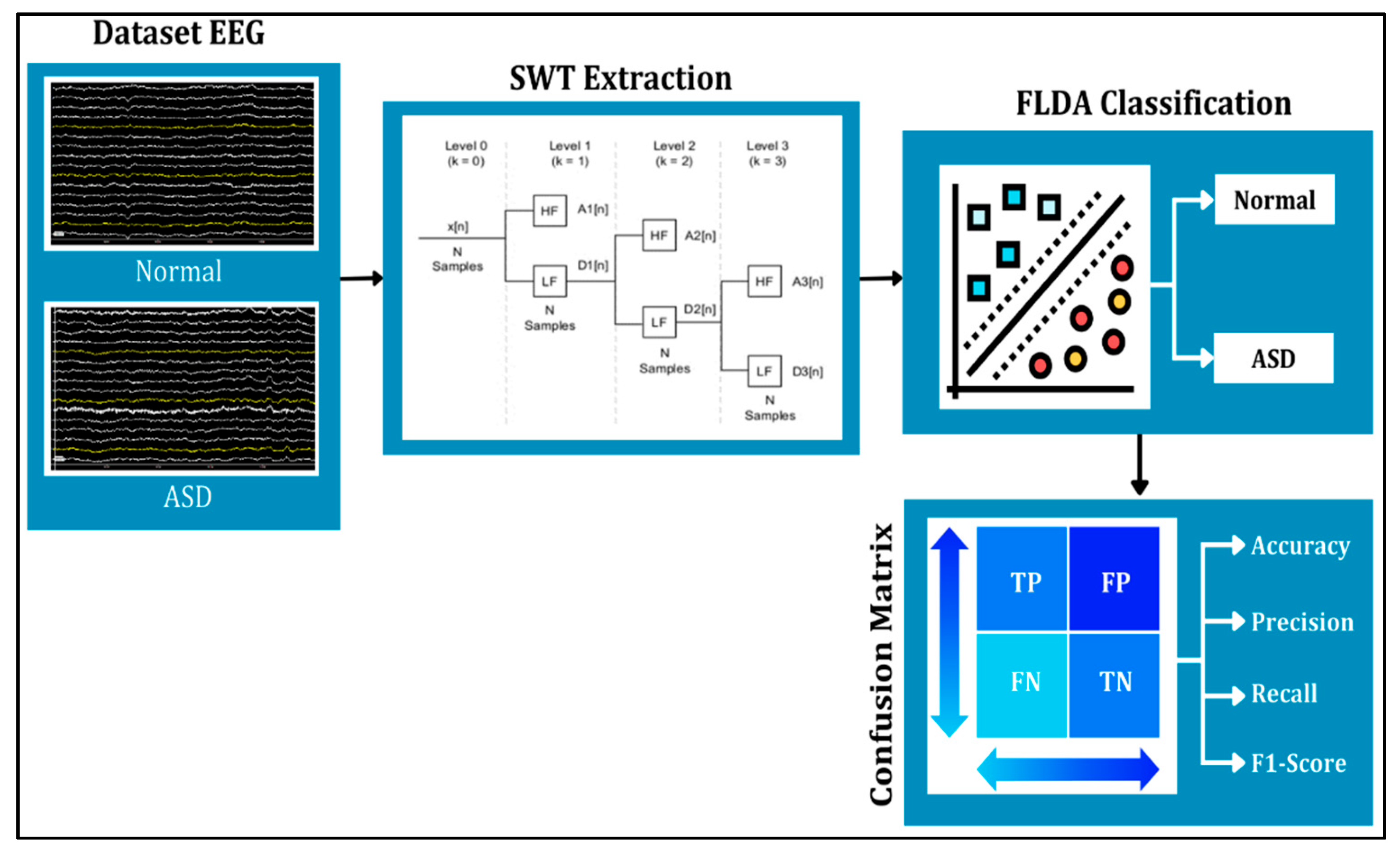
Figure 2.
SWT Processing Method.
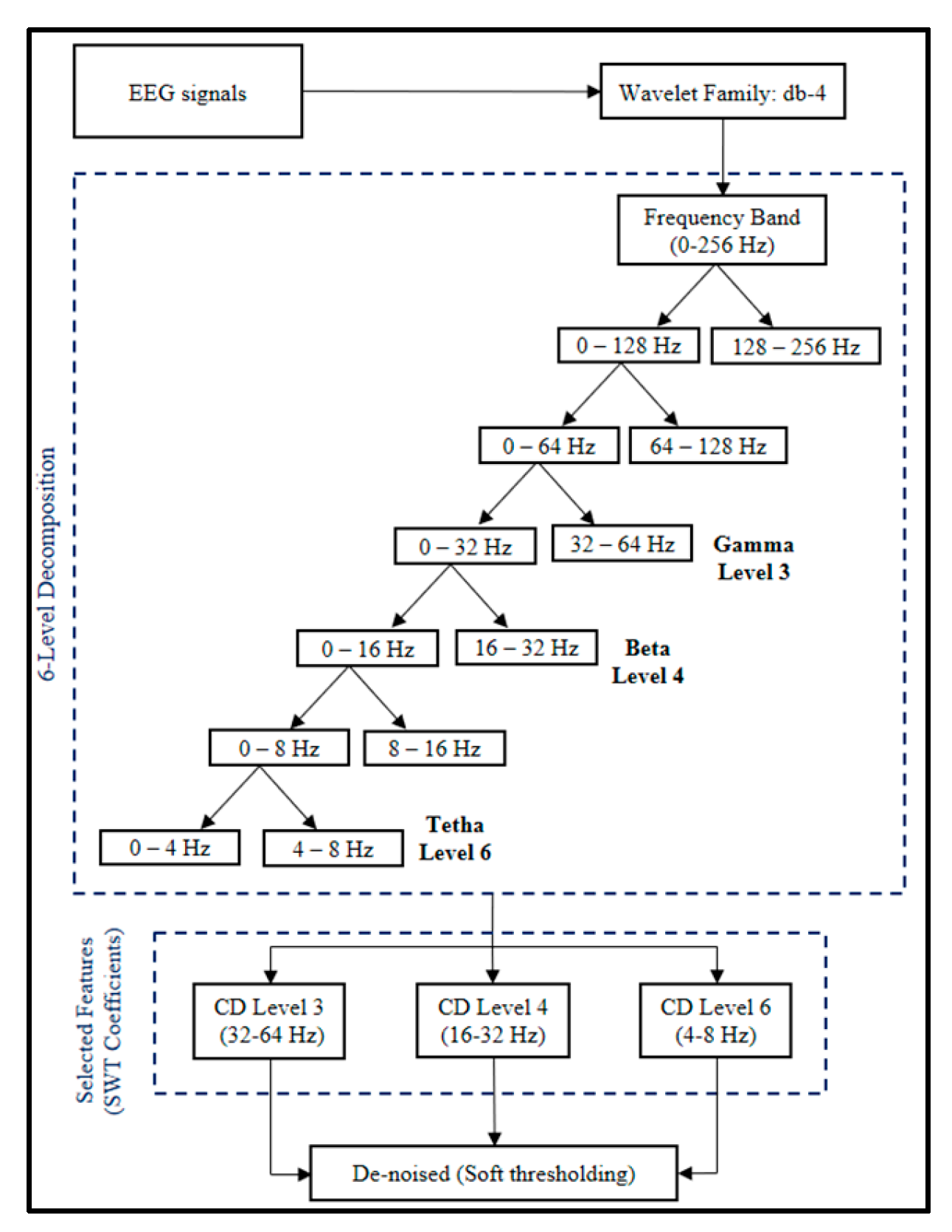
Figure 3.
FLDA System Performance Setting.
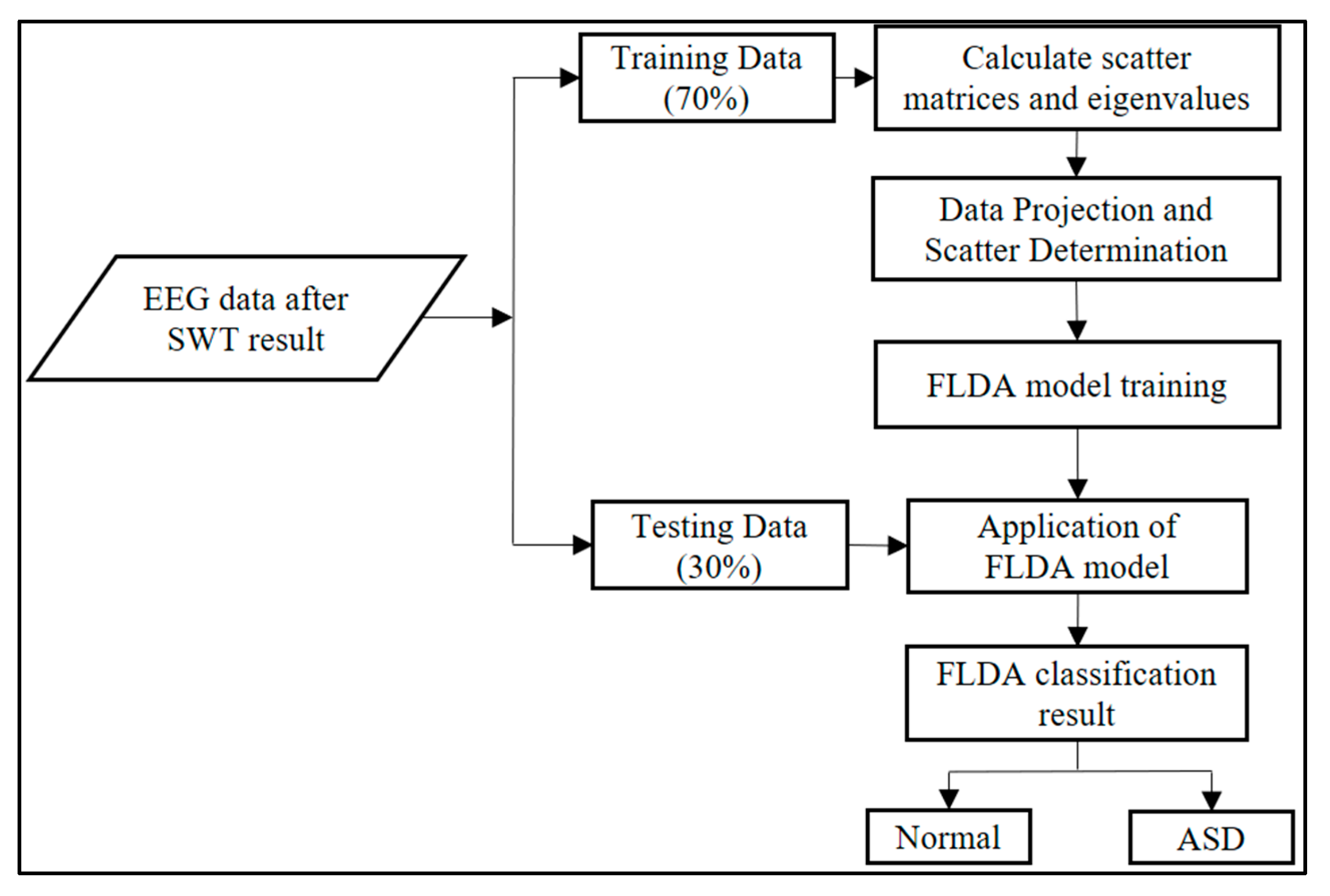
Figure 4.
Result of FLDA classifications: (a) normal class and (b) autism class.
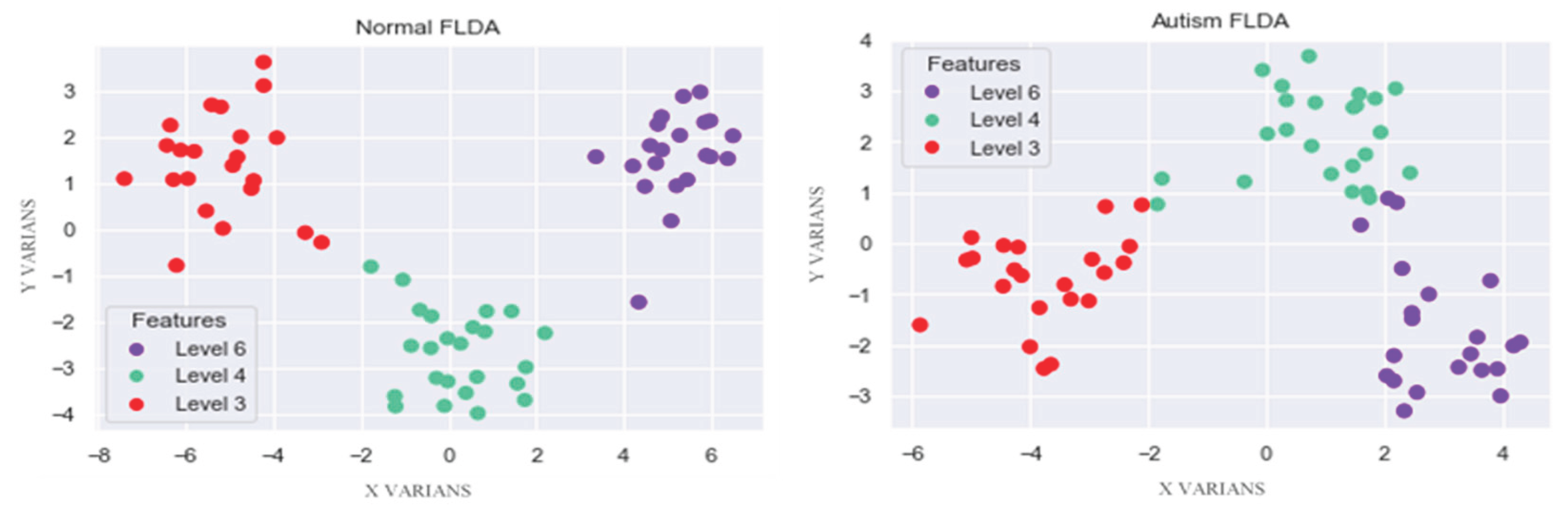

Table 1.
Extraction and denoising result of normal EEG features at Level 3.
| Data | FP1 (Hz) | F3 (Hz) | F7 (Hz) | T3 (Hz) | … | OZ (Hz) | Class |
|---|---|---|---|---|---|---|---|
| 1 | 20.70515 | 21.71104 | 20.39143 | 6.959006 | … | -10.174 | Normal |
| 2 | 22.19637 | 24.09438 | 22.9614 | 12.63111 | … | -15.6247 | Normal |
| 3 | 24.53501 | 25.39331 | 24.71271 | 16.85653 | … | -17.9162 | Normal |
| … | … | … | … | … | … | … | … |
| 8.000 | 25.94938 | 26.05881 | 24.2168 | 12.1017 | … | -15.0655 | Normal |
Table 2.
Extraction and denoising result of normal EEG features at Level 4.
| Data | FP1 (Hz) | F3 (Hz) | F7 (Hz) | T3 (Hz) | … | OZ (Hz) | Class |
|---|---|---|---|---|---|---|---|
| 1 | 20.17439 | 21.08247 | 19.67696 | 7.651534 | … | -10.0963 | Normal |
| 2 | 21.38831 | 23.34116 | 21.87948 | 13.52822 | … | -15.165 | Normal |
| 3 | 23.45923 | 24.5291 | 23.34335 | 17.9128 | … | -17.1389 | Normal |
| … | … | … | … | … | … | … | … |
| 8000 | 24.60603 | 25.12293 | 22.6783 | 13.30784 | … | -13.937 | Normal |
Table 3.
Extraction and denoising result of normal EEG features at Level 6.
| Data | FP1 (Hz) | F3 (Hz) | F7 (Hz) | T3 (Hz) | … | OZ (Hz) | Class |
|---|---|---|---|---|---|---|---|
| 1 | 20.29084 | 20.7321 | 19.22691 | 7.560314 | … | -9.21138 | Normal |
| 2 | 21.54138 | 22.65318 | 21.23181 | 13.1909 | … | -13.8999 | Normal |
| 3 | 23.58845 | 23.79831 | 22.53498 | 17.41969 | … | -15.6655 | Normal |
| … | … | … | … | … | … | … | … |
| 8.000 | 24.09664 | 24.48455 | 21.55254 | 12.73626 | … | -12.8648 | Normal |
Table 4.
Extraction and denoising result of ASD EEG features at Level 3.
| Data | FP1 (Hz) | F3 (Hz) | F7 (Hz) | T3 (Hz) | … | OZ (Hz) | Class |
|---|---|---|---|---|---|---|---|
| 1 | 6.332813 | -22.1256 | -12.8341 | 7.169845 | … | 19.57307 | ASD |
| 2 | 0.626899 | -21.0605 | -12.1656 | 3.108195 | … | 12.88358 | ASD |
| 3 | -0.77898 | -17.5857 | -17.161 | 3.075867 | … | 15.92139 | ASD |
| … | … | … | … | … | … | … | … |
| 8.000 | 14.84071 | -6.8033 | -7.82897 | 6.833994 | … | 16.34017 | ASD |
Table 5.
Extraction and denoising result of ASD EEG features at Level 4.
| Data | FP1 (Hz) | F3 (Hz) | F7 (Hz) | T3 (Hz) | … | OZ (Hz) | Class |
|---|---|---|---|---|---|---|---|
| 1 | 6.586297 | -22.0628 | -12.5653 | 8.17759 | … | 19.45576 | ASD |
| 2 | 1.226708 | -21.3885 | -11.5433 | 4.327005 | … | 13.16418 | ASD |
| 3 | 0.124645 | -18.2795 | -16.2514 | 4.390527 | … | 16.547 | ASD |
| … | … | … | … | … | … | … | … |
| 8.000 | 16.14102 | -8.07165 | -6.58169 | 7.992751 | … | 17.45375 | ASD |
Table 6.
Extraction and denoising result of ASD EEG features at Level 6.
| Data | FP1 (Hz) | F3 (Hz) | F7 (Hz) | T3 (Hz) | … | OZ (Hz) | Class |
|---|---|---|---|---|---|---|---|
| 1 | 6.57135 | -22.081 | -12.5781 | 7.771396 | … | 19.67485 | ASD |
| 2 | 1.582899 | -21.7472 | -11.0373 | 4.023141 | … | 13.54433 | ASD |
| 3 | 0.970091 | -18.8331 | -14.6427 | 4.929182 | … | 17.00702 | ASD |
| … | … | … | … | … | … | … | … |
| 8.000 | 17.42998 | -8.73002 | -5.08022 | 9.285977 | … | -18.1207 | ASD |
Table 7.
Result of the confusion matrix calculation for normal EEG.
| EEG Normal | Prediction | |||
|---|---|---|---|---|
| Level 3 | Level 4 | Level 6 | ||
| Actual | Level 3 | 2,975 | 50 | 0 |
| Level 4 | 119 | 3,685 | 101 | |
| Level 6 | 0 | 87 | 983 | |
Table 8.
Extraction and denoising result of ASD EEG features at Level 6.
| Class | SWT | Precision | Recall | F1-Score | Accuracy |
|---|---|---|---|---|---|
| Normal | Level 3 | 0.96 | 0.98 | 0.97 |
96% |
| Level 4 | 0.96 | 0.94 | 0.95 | ||
| Level 6 | 0.91 | 0.92 | 0.91 |
Table 9.
Result of the confusion matrix calculation for ASD EEG.
| ASD EEG | Prediction | |||
|---|---|---|---|---|
| Level 3 | Level 4 | Level 6 | ||
| Actual | Level 3 | 1,862 | 261 | 68 |
| Level 4 | 196 | 5,363 | 3 | |
| Level 6 | 0 | 54 | 193 | |
Table 10.
The result of the confusion matrix for ASD EEG.
| Class | SWT | Precision | Recall | F1-Score | Accuracy |
|---|---|---|---|---|---|
| Autism | Level 3 | 0.90 | 0.85 | 0.88 | 93% |
| Level 4 | 0.94 | 0.96 | 0.95 | ||
| Level 6 | 0.73 | 0.78 | 0.76 |
Disclaimer/Publisher’s Note: The statements, opinions and data contained in all publications are solely those of the individual author(s) and contributor(s) and not of MDPI and/or the editor(s). MDPI and/or the editor(s) disclaim responsibility for any injury to people or property resulting from any ideas, methods, instructions or products referred to in the content. |
© 2025 by the authors. Licensee MDPI, Basel, Switzerland. This article is an open access article distributed under the terms and conditions of the Creative Commons Attribution (CC BY) license (http://creativecommons.org/licenses/by/4.0/).
Copyright: This open access article is published under a Creative Commons CC BY 4.0 license, which permit the free download, distribution, and reuse, provided that the author and preprint are cited in any reuse.


