
Submitted:
21 August 2024
Posted:
21 August 2024
You are already at the latest version
Abstract
We used numerical methods to define the normative structure of the different stages of sleep and wake (W) in a pilot study of 19 subjects without pathology (18–64 years old) using a double-banana bipolar montage. Artefact-free 120–240 s epoch lengths were visually identified and divided into 1 s windows with a 10% overlap. Differential channels were grouped into frontal, parieto-occipital, and temporal lobes. For every channel, the power spectrum (PS) was calculated via fast Fourier transform and used to compute the areas for the delta (0–4 Hz), theta (4–8 Hz), alpha (8–13 Hz), and beta (13–30 Hz) bands, which were log-transformed. Furthermore, Pearson’s correlation coefficient and coherence by bands were computed. Differences in logPS and synchronization from the whole scalp were observed between the sexes for specific stages. However, these differences vanished when specific lobes were considered. Considering the location and stages, the logPS and synchronization vary highly and specifically in a complex manner. Furthermore, the average spectra for every channel and stage were very well defined, with phase-specific features (e.g., the sigma band during N2 and N3, or the occipital alpha component during wakefulness), although the slow alpha component (8.0–8.5 Hz) persisted during NREM and REM sleep. The average spectra were symmetric between hemispheres. The properties of K-complexes and the sigma band (mainly due to sleep spindles – SSs) were deeply analysed during the NREM N2 stage. The properties of the sigma band are directly related to the density of SSs. The average frequency of SSs in the frontal lobe was lower than that in the occipital lobe. In approximately 30% of patients, SSs showed bimodal components in anterior regions. qEEG can be easily and reliably used to study sleep in healthy subjects and patients.
Keywords:
bipolar montage
; coherence
; fast Fourier transform
; K-complex
; Pearson’s correlation coefficient
; Polysomnography
; power spectra
; qEEG
; sleep spindles
; sleep staging.
1. Introduction
Sleep in humans is a behavioural state that alternates with waking, relative to which it is characterized by attenuation of motor output, an increased threshold to sensory input, typical changes in central and peripheral physiology, stereotypic postures, relatively easy reversibility (distinguishing it from coma) and diminished conscious awareness, although some kind of consciousness can be obtained during the rapid eye movement state (REM), in which dreaming takes place [1,2].
However, sleep is not a uniform state. In contrast, it is composed of different well-coordinated stages and is regulated by different brain structures located at the brainstem, diencephalon, thalamus and cerebral cortex. In fact, this is an active state promoted by complex neural networks that are finely tuned. Normal human sleep comprises two distinct states: nonrapid eye movement (NREM) and REM sleep. In turn, NREM sleep is composed of three different stages: stage 1 NREM (N1), stage 2 NREM (N2), and stage 3 NREM (N3). Overall, NREM sleep accounts for 75–80% of sleep time. N1 sleep comprises 3–8% of sleep time. This phase occurs most frequently in the transition from wakefulness to sleep stages or following arousals. In stage N1 sleep, alpha activity diminishes, and a low-voltage, mixed-frequency pattern appears. Vertex sharp waves (VSW, 50–200 ms) are prominent towards the end of this phase. The N2 stage comprises 45–55% of the total sleep time. The typical findings include sleep spindles (SSs) and K-complexes (KCs). An SS is a 12–14 Hz waveform lasting at least 0.5 s, having a wax and waning appearance with a main location generalized with a maximum at fronto-central regions, and it is generated within thalamic reticular neurons that produce inhibitory sequences on thalamocortical cells [3,4]. A KC is a waveform with two components (a negative wave followed by a positive wave), both of which last more than 0.5 s and are generated intracortically [5]. KCs are generalized with a maximum at the vertex [6]. Delta waves (1–4 Hz) in the EEG may first appear at N2 sleep but in small amounts. Stage N3 accounts for 15–20% of the total sleep time and constitutes slow-wave sleep, characterized by moderate to large amounts of high-amplitude, slow-wave activity. Finally, REM sleep accounts for 20–25% of sleep time. EEG tracings are characterized by low-voltage, mixed-frequency activity with slow alpha (defined as 1–2 Hz slower than wake alpha) and theta waves. REM sleep can be divided into tonic (desynchronized EEG, atonia and suppression of reflexes) and phasic sleep, characterized by rapid eye movements in all directions [5,7]. Moreover, transient changes in heart rate, tongue movements, myoclonic twitching of the chin and limb muscles, and penis and clitoris erection are observed. Sawtooth waves, with a frequency in the theta range, involve the appearance of teeth on the cutting edge of a saw blade and often occur in conjunction with rapid eye movements.
The transitions from wakefulness to NREM sleep and from NREM to REM sleep are regulated by brain-stem, hypothalamus and diencephalic structures [1,2,5,7,8], and although brain-stem nuclei are involved in eye-ball movements and muscle tone, it is important to note that the latter can be considered epiphenomena and do not regulate the state of sleep.
Polysomnography (PSG) is the gold standard method for evaluating sleep in humans [9]. The minimum number of EEG channels recommended by the American Academy of Sleep Medicine is three, i.e., F4-M1, C4-M1 and O2-M1, although backup electrodes should be placed at F3-M2, C3-M2 and O1-M2. Other acceptable montages should be Fz-Cz and Cz-Oz with backup electrodes at Fpz, C3, O1 and M1. All the electrodes were placed according to the 10-20 International System. Additional electrodes are used to identify eye movements (electro-oculogram, EOG) and are placed approximately 1 cm from the edge of the eye and chin electrodes to record electromyography (EMG) [10]. Accessory electrodes help to stage sleep, but this is likely because the interpretation of EOG and EMG signals is simpler than that of EEG recordings collected from 19 channels.
In the literature, numerous papers have described numerical methods of diverse difficulty in describing partial aspects of sleep, such as KCs or SSs [11,12], transitions between phases [14,15,16], or those featuring pathologies [17,18], but few of them have been devoted to the sleep stage [19,20]. To the best of our knowledge, no comprehensive description of frequency composition, synchronization features and typical waveform properties in a whole scalp approach has been provided. Similar papers describing the spectral power structure in healthy humans date back more than 40 years [21,22].
In this work, we assessed two complementary goals: i) the numerical characterization of the wake and sleep stages across the whole scalp, including the power spectra structure and synchronization, and ii) revisiting the properties of KCs and SSs, in both cases, using the most common montage used in clinical practice (i.e., bipolar double banana). Therefore, our goal is not to test the suitability of staging sleep with a new method but rather to describe the numerical properties of physiological sleep and assess the discriminability of spectral and synchronization properties across all sleep phases. A positive and clear definition of physiological sleep is needed for subsequent studies on pathologies.
The abbreviations used are listed at the end of the manuscript.
2. Materials and Methods
2.1. Patients
The Materials and Methods should be described with sufficient details to allow others to replicate and build on the published results. Please note that the publication of your manuscript implicates that you must make all materials, data, computer code, and protocols associated with the publication available to readers. Please disclose at the submission stage any restrictions on the availability of materials or information. New methods and protocols should be described in detail while well-established methods can be briefly described and appropriately cited.
Research manuscripts reporting large datasets that are deposited in a publicly available database should specify where the data have been deposited and provide the relevant accession numbers. If the accession numbers have not yet been obtained at the time of submission, please state that they will be provided during review. They must be provided prior to publication.
Interventionary studies involving animals or humans, and other studies that require ethical approval, must list the authority that provided approval and the corresponding ethical approval code.
In this study, we retrospectively analysed the recordings obtained from 9 men (33.4 ± 3.9 years old) and 10 women (31.3 ± 5.1 years old) referred for video-electroencephalography (vEEG) at the National Reference Unit for the Treatment of Refractory Epilepsy, University Hospital La Princesa (Spain), from 2018 to 2023. From a total of 494 patients evaluated, we selected those patients whose results were obtained via physiological recording. These patients, without organic pathology, were referred for the assessment of possible paroxysmal events, i.e., epilepsy, nonepileptic psychogenic seizures or cardiovascular events [23]. No epilepsy, encephalopathy, focal slowing or any other anomalous waveforms were observed. Therefore, the resting state, active awake state and all the sleep stages presented physiological properties. The experimental procedure was approved by the medical ethical review board of the Hospital Universitario de La Princesa (ref 5548) and was deemed “care as usual”. Under these circumstances, written informed consent was not needed.
2.2. EEG Recording and Sleep Staging
vEEG was performed via a 64-channel digital VEEG system (EMU64, NeuroWorks. XLTEK®, Oakville, Canada) with 19 scalp stainless steel electrodes fixed with collodion according to the 10–20 international system; electrocardiography (ECG) and simultaneous video images were recorded continuously for 24 h. If needed, one or two EMGs in the limbs/shoulders were also added. Electrodes F7 and F8 were used for EOG recording and were referred to A1 for the sleep stage. No chin EMG was used.
Recordings were performed at a 512 Hz sampling rate with a 0.5–70 Hz bandwidth for EEG and EOG, with a 50 Hz notch on. The EMG bandwidth was 1.5–200 Hz, notch on, and the ECG bandwidth was 1.5–30 Hz, notch on. The impedance for EEG was under 25 kΩ. Artefact-free periods of at least 4 min were selected for analysis, except for the N1 stage, where the minimum period of analysis was 2 min.
Wake (W): physiological eye-closed resting-state EEG (rsEEG; [24]) with antero-posterior gradient and occipital wax and waning alpha rhythm.
N1 stage: alpha activity diminishes, and a low-voltage, mixed-frequency pattern appears. Vertex sharp waves (50–200 ms) are prominent towards the end of this phase.
N2 stage: no antero-posterior gradient, moderate amplitude mixed frequencies with the presence of SSs described as a 12–14 Hz waveform (the frequency band between 10 and 16 Hz is denoted as the sigma band) lasting at least 0.5 s, having a waxing and waning appearance with a main location generalized with a maximum at central derivations [10], and KCs, a waveform with two components (a negative wave followed by a positive one), both lasting more than 0.5 s, generalized through the scalp with a maximum at the forehead.
N3 stage: This stage involves slow-wave sleep and is characterized by moderate to large amounts of high-amplitude, slow-wave activity at 1 Hz.
REM sleep stage: Tracings are characterized by low-voltage, mixed-frequency activity with slow alpha (defined as 1–2 Hz slower than wake alpha) and theta waves. REM sleep can be divided into tonic (desynchronized EEG, atonia and suppression of reflexes) and phasic (characterized by rapid eye movements in all directions) phases. Moreover, transient changes in heart rate are observed. Sawtooth waves, with a frequency in the theta range, involve the appearance of teeth on the cutting edge of a saw blade.
2.3. Numerical Analysis
The numerical method used for qEEG has been previously described in detail [24,25,26]. Briefly, different lengths of raw records were exported from the EEG device to the ASCII file. Artefacts were excluded by the export of several artefact-free chunks, which were later combined for analysis. Although the raw recordings were digitized at 512 Hz, we downsampled them to 256 Hz. Exported files were digitally filtered by a sixth-order Butterworth digital filter between 0.5 and 30 Hz.
A differential EEG double-banana montage was reconstructed. The topographic placement of channels was defined on the scalp as the midpoint between the electrode pairs defining the channel, e.g., the Fp1–F3 channel would be placed at the midpoint of the geodesic between the Fp1 and F3 electrodes.
All recordings were divided into 1 second moving windows with 10% overlap. The total length used during the fast Fourier transform (FFT) is directly related to the frequency precision in the power spectrum (PS). Overlap was used to minimize the effect produced by windowing. These features give rise to a maximum frequency sensitivity of 0.5 Hz.
For each window and frequency, we computed the discrete FFT of the voltage obtained from every channel to obtain the PS (in µV2/Hz). We also computed Shannon’s spectral entropy (SSE).
We used the classical segmentation of EEG bands (in Hz), delta (δ): 0.5-4, theta (θ): 4-8, alpha (α): 8-13 and beta (β): 13-30. Special attention was given to the so-called sigma band (σ): 10-15.
The different EEG bands are rooted in different neural systems; therefore, the synchronization of different bands can offer specific information. Linear synchronization in the time domain was assessed by Pearson’s correlation coefficient (ρ). A very useful method to assess specific band synchronization in the frequency domain is coherence (Coh) [27,28].
The mean values of all windows for ρ and Coh were computed, and the mean correlation and coherence matrices were obtained. The mean values of synchronization for hemispheres and lobes were computed as the average of all pairs () of channels (), according to this expression , for hemispheres.
The spectral and synchronization variables were topographically grouped into hemispheres and lobes. In the case of the left hemisphere (shown as an example), we grouped for frontal , parieto-occipital , and temporal . For the whole left hemisphere, we used the expression . Channels from the right hemisphere were grouped accordingly.
Numerical analysis of the EEG recordings was performed with custom-made MATLAB® software (MathWorks, Natick, MA, USA).
2.4. Analysis of Typical Waveforms of Sleep
The features of a transient waveform are the number of phases, amplitude, duration and scalp location. These properties are easily measured for KCs but are more difficult for SSs because the start and end are difficult to identify, as is the amplitude.
To define the properties of sleep waveforms, we visually identified, by a clinical neurophysiologist with more than 20 years of experience, a minimum of 25 (sometimes up to 35) well-defined instances during the characteristic stages of appearance. We exported periods of 12 seconds centred at the maximum amplitude of the KCs. We then average all the elements marked to obtain an average KC (aKC; see Appendix, Figure A1A). We measured the amplitude (; in µV) and duration ( of both phases (Figure 1A) of this aKC. In the case of SSs, instead of measuring times and amplitudes on an averaged SS, which could be difficult because of the absence of a clearly defined and constant amplitude and temporal limits, we computed the average PS (aPS) of 30 instances (5 s in length) to identify the maximum power (mP) and peak frequency (pF) for the σ component (Figure A1B).
2.5. Differences between the Mean Spectra
To compare the aPSs of the channels, we normalized all the PSs to the area of the PS obtained for the Cz-Pz channel during wakefulness. Therefore, the proportion between spectra for different phases was maintained, but absolute values were removed.
We had a total of 5 aPSs for every channel (e.g., W, N1, N2, N3 and REM). Every aPS can be considered a function; then, we have five functions . We computed the absolute difference between all the functions for every channel () according to the following equation:
where the domain is the frequency .
2.6. Numerical Model of the Density of Sleep Spindles
To assess an estimation of the SS density and its relationship with the σ component, we performed a numerical simulation with a controlled density of SSs, measured as the percentage of SSs over a defined period. We exported 50 chunks (2 s each) of the N2 stage without SSs and another 50 periods, including a well-defined SS. We randomly selected different proportions of SSs, namely, 0, 25, 50, 75 and 100%. We computed the aPS for these periods of 100 s and later measured the pF and mP for the σ band at channels Fp1-F3/Fp2-F4 (fronto-polar) and Fz-Cz (anterior midline).
2.7. Statistics
Evidently, the absolute values of the PS are quite different from patient to patient; therefore, it is not useful to compare the raw values. Therefore, we used a log transform (Pastor 2023 [24,29]) for the PS measures (logPS). The synchronization measures and SSE were compared in terms of their raw values.
Statistical comparisons between groups were performed via Student’s t test or ANOVA for normally distributed data. Normality was evaluated via the Kolmogorov–Smirnov test. The Mann–Whitney rank sum test or Kruskal‒Wallis one-way analysis of variance on ranks was used when normality failed. In the last case, the Tukey test was used for all pairwise post hoc comparisons of the mean ranks of the treatment groups. Comparisons between the same lobes from different stages were assessed through paired Student’s t tests. SigmaStat® 3.5 software (SigmaStat, Point Richmond, CA, USA) and MATLAB® were used for statistical analysis.
Descriptive statistics are presented as the mean ± SEM (for Gaussian distributions) or median (Med), and the interpercentile range IP25-75 (percentile 25, percentile 75) for non-Gaussian distributions.
Quadratic nonlinear regression was performed via the least-square method, and r was used to study the dependence between variables. Statistical significance was evaluated via a contrast hypothesis against the null hypothesis ρ = 0 via the following formula:
This describes a one-tailed t-Student distribution with n − 2 degrees of freedom [30].
SigmaStat® 3.5 software (SigmaStat, Point Richmond, CA, USA) and MATLAB® were used for statistical analysis.
The significance level was set at p = 0.05.
3. Results
3.1. Sleep Staging
3.2. Sex Dependence and Symmetry between Hemispheres
Before analysing the changes in variables between sleep phases, we addressed the general properties for both sexes because it has been shown that females present higher absolute spectral densities [31]. In Table 1, we present the whole-scalp logPS, Coh (including in the same stage δ, θ, α and β) and ρ for both sexes.
The whole-scalp average for logPS was lower for the W stage and greater for the N3 and REM stages, whereas the whole-scalp average for Coh (computed for all the bands) was lower for women at the W, N1 and N2 stages. No differences in whole-scalp averages for ρ were observed.
Despite the differences observed for global magnitudes, when we compared the same regions and stages between men and women, as shown in Figure 2, neither differences for any sleep phase nor for any frequency, SSE or synchronization between males and females were observed.
Figure 2 shows that frontal power tends to be lower in the theta, alpha and beta bands than in the other lobes of the same band.
Considering the absence of differences in paired lobes between males and females, we combined values from both sexes.
We also compared the symmetry between the same lobes on both sides (right and left). All of these data are presented in Appendix B, Table B1. No differences between paired lobes were observed. Therefore, the values from the right and left hemispheres were grouped for subsequent analysis.
3.3. Comparison of the Average logPS by Phase and Lobe
Figure 3 shows the power of all the bands (δ, θ, α and β) for the different lobes (F, PO and T) through the stages from the wake (W; Figure 3A) to the REM sleep stage (Figure 3E). We compared the differences for the same band over the entire scalp (horizontal lines) and the different configurations at the same lobe of all the bands (e.g., from δ to β in the F lobe), the statistical significance of which is indicated by pairs of asterisks. Each band is indicated in a specific colour (black = δ; red = θ; blue = α and green = β), the coloured lines indicate differences between a pair of lobes of the same band, and the asterisks indicate significant differences between pairs of bands in the same lobe.
Interestingly, the differences between bands for the same stage were greater during the W (θ, α and β) and N1 (θ and α) phases, although no differences between the PO and T lobes were observed. These differences vanished during the N2 stage, where only a difference between the F and PO lobes for the θ band was observed. The N3 sleep stage was the more homogeneous phase because all the lobes had the same power, which was obviously dominated by the δ band, although the remaining bands were equally similar between the scalp areas. The REM stage ultimately revealed a difference between the F and PO and the F and T lobes for the α band as well as a difference between the F and PO lobes for the θ band. These significant differences can be clearly understood from the power spectra shown in the right column of Appendix Figure 2A. Figure 3F shows that the theta bands in the W and REM stages were the same but completely different in the alpha band.
Considering every phase, the pairs of significant differences followed the next order, from highest to lowest: N3 > REM > N2 > N1 = W.
Regarding differences between bands measured at the same stage and lobe, it is clear that the lower differences were for T lobes, probably because the dispersion was greater in this region. For each lobe, there is a maximum of 6 pairs of different bands (i.e., δ/θ, δ/α,…α/β) and 5 stages (from W to REM); therefore, the maximum number of different pairs is 6 × 5 = 30. The differences are shown in Table 2.
Considering all the stages, the differences were greater for F lobes, followed by PO and finally T. For the F lobe, all the combinations, including the δ band, were different from the rest of the bands for all the stages and very similar for the PO and T lobes. The δ band was obviously the most variable across the dynamics of wake-sleep. However, the less different pair of bands was α/β, which was significant mainly for the F lobe (60% of cases), and nothing at all for the T lobe.
3.4. Comparison of Synchronization by Phases and Lobes
In addition, PS changes for every stage in terms of both the power of the bands and the scalp distribution. We addressed the changes in the two linear measurements of synchronization used. In this case, synchronization was measured not only for every lobe but also for all the channels of the same hemisphere. Figure 4 shows the synchronization measured through Coh of all the bands and lobes through the stages, considering the global coherence (Figure 4A) and the distribution across the scalp from wake (Figure 4B) to REM sleep stages (Figure 4E). We compared the differences for the same band over the entire scalp (horizontal lines) and the different configurations at the same lobe of all the bands (e.g., from δ to β in the F lobe), the statistical significance of which is indicated in pairs of coloured asterisks.
Figure 4A shows that there was a difference between N3 and the W as well as N1 and REM stages for the δ, θ and α bands (3 pairs on 10 possibilities). Therefore, the global coherence was similar for W, N1 and N2, and for N2 and N3. The coherence of the β band was quite similar for all the phases. No difference between δ and θ coherence was observed for any phase, but all the stages showed a difference between the δ/α and δ/β θ/α pairs. The β band showed the lowest global coherence for all the phases.
Next, we analysed the structure of coherence across the scalp and for all the phases. Interestingly, the differences between bands for the same stage were greater during the N2 (all four bands) and N3 (all four bands) phases, with differences between F and PO and between T and PO but not between F and T. The REM sleep phase also presented differences for all four bands but no difference between the F and PO lobes for the α band. The W stage was the most homogeneous phase, and only differences for the F and PO as well as PO and T lobes for the beta band were observed.
Considering every phase, the pairs of significant differences followed the same order observed for logPS, which, from highest to lowest, was N3 > REM > N2 > N1 = W.
Regarding differences between bands measured at the same stage and lobe, it is clear that the lower differences are for T lobes, probably because the dispersion is greater in this region, as we observed for the PS (Figure 3). The differences are shown in Table 3.
Considering all the stages, the differences were greater for F lobes, followed by PO and finally T. For the F lobe, all the combinations, including the β band, were different from the rest of the bands for all the stages. The β band was obviously the most variable across the dynamics of wake-sleep. However, the less different pair of bands was δ/θ.
Although they share some common features, the structures of logPS and coherence clearly differ, indicating that both properties are independent across the different stages of sleep.
Coherence is a measure in the dominance of frequency, but in the dominance of time, the measure used was ρ. We analysed its properties in Figure 5.
Figure 5A shows that the difference between phases was greater than that for coherence. In fact, ρ detected differences in 6/10 pairs of phases, instead of the 3/10 detected by coherence. We observed differences between W/N2, W/N3, N1/N2, N1/N3, N2/N3 and N3/REM; therefore, the stage with the greatest difference was N3, whereas REM differed only once, with N3.
Additionally, the correlation by phases and across the scalp was addressed. Interestingly, the differences between the bands for all the sleep stages were similar between F/PO and PO/T but not for F/T. Conversely, no difference was observed across the scalp during the W phase. Globally, sleep is characterized by a decrease in the correlation between the PO lobe and an increase in the variability in the T lobe. However, obviously, the magnitude of correlation could change for every lobe along the phases. To evaluate this possibility, we plotted the magnitude of correlation for every lobe and for all the phases (Figure 6). For the F lobe, we obtained 4 pairs that were significantly different: only 2 pairs for the PO lobe and another 2 pairs for the T lobe. Interestingly, the N1/N3 pair was different for all three lobes. Interestingly, the dynamics across the phases were similar for the F and T lobes (with greater variance in the last lobe) but completely different for the PO lobe.
In summary, the structure of synchronization, measured by ρ and coherence, is highly complex, changing from phase to phase and from lobe to lobe. In both cases, the maximum value of synchronization was achieved during the N3 sleep stage.
3.5. Mean Power Spectra across the Scalp
We computed the aPS normalized to the channel Cz-Pz at the W state, computed as a grand average from all the patients. The global structure (i.e., the relationship between bands for every channel and through channels) was completely similar between both hemispheres. Figure 7 shows that the aPSs were completely different between the phases. We can observe how the posterior dominant rhythm (peaked at 10 Hz) decreases and slows during the N1 sleep stage, with a peak at 8.0 Hz, while maintaining a 10 Hz component only in the occipital lobes. During the N2 stage, a prominent delta band appears, which is even greater for the N3 stage. During the N2 stage, the σ power reached a maximum at approximately 13 Hz, and the θ component was lower at 7.5 Hz. During the N3 phase, the σ power was also evident but was slower than that in N2, with a mean peak at approximately 12.0 Hz (slow SS), and the theta 7.5 Hz component practically disappeared. Finally, during REM sleep, a small alpha component at 8.0–8.5 Hz (slow alpha) can be observed with the absence of the σ band.
We computed the maximum difference (maxΔh) between pairs of normalized PSs (see Equation (1)). In this way, we could identify the region of the scalp where the difference was higher and lower for all the sleep and W phases (Figure 8).
We did not find differences between hemispheres; although we observed a nonsignificant tendency for higher values in the left channel (p = 0.442; for the Mann‒Whitney rank sum test), we observed great symmetry between the lobes. In fact, the linear regression between the left and right hemispheres fit very well to a straight function (r = 0.9839; p < 10-4, Student’s t test). We computed the average of the paired channels (e.g., (Fp1-F3+Fp2-F4)/2)) to compare with the midline channels. From these values, we observed that there were two different regions in the scalp: one with values of maxΔh > 50, including the channels Cz-Pz (76.74), P3-O1/P4-O2 (74.79), T3-T5/T4-T6 (71.37) and F7-T3/F8-T4 (69.61), and the rest of the scalp, with values maxΔh < 40, with the lowest values at F3-C3/F4-C4 (25.64), C3-P3 (30.69) and T5-O1/T6-O2 (35.72).
3.6. KC and SS Distributions across the Scalp
We analysed the properties of the KCs and SSs across the scalp. Figure 9A shows an aKC (obtained from 32 individual KCs). The amplitude is frontal regions and lower in the occipital lobe. The amplitude from the aKC for both phases is shown in Figure 9B. The error bars are the confidence intervals (CIs); therefore, taking into account that the distribution fit well to a Gaussian distribution, the amplitude was significant when the CI did not cross the 0 level. Interestingly, (Figure 9B), the aKC did not reach statistical significance at frontopolar regions (Fp1-F3/Fp2-F4), with the maximum amplitude at frontal lobes (F3-C3/F4-C4, 58.0 ± 3.8 and 55.3 ± 3.8 µV, respectively, peak-to-peak) and the lower amplitude at parieto-occipital channels (P3-O1/P4-O2, 26.2 ± 2.7 and 22.4 ± 2.1 µV, respectively, statistically significant). However, the KCs not only showed an antero-posterior gradient in the parasagittal region but also on the lateral side. In this case, the highest value was observed in the frontopolar lateral region (Fp1-F7/Fp2-F8, 65.0 ± 4.6 and 62.5 ± 3.6 µV, respectively), with the lowest value in the temporo-occipital region (T5-O1/T6-O2, 7.4 ± 1.4 and 11.7 ± 1.5 µV, respectively, both statistically significant). At the midline, the gradient was not as evident, with practically the same value in the frontal as in the parietal regions (61.6 ± 5.0 for Fz-Cz and 56.0 ± 3.8 for Cz-Pz). The total duration (d1 + d2) of aKC (Figure 9C) was similar to the amplitude, with a maximum duration in the lateral fronto-polar regions (Fp1-F7/Fp2-F8, 0.92 ± 0.07 and 0.95 ± 0.04 s, respectively), with a minimum duration in the temporo-occipital channels (T5-O1/T6-O2, 0.30 ± 0.04 and 0.48 ± 0.05 s, respectively). The correlations between both phases were highly significant (Student’s t test), as can be observed for V1/V2 (Figure 9D; r = 0.965, p < 10-4), d1/d2 (Figure 9E; r = 0.898, p < 10-4), V1/d1 (Figure 10F; r = 0.675, p = 0.002) and V2/d2 (Figure 10G; r = 0.753, p = 0.0003).
From Figure 9D and Figure 9E, we can obtain the constitutive equations describing the canonical structure of the KCs. The equation relating the amplitude of both components can be described as , and for the durations, . These properties can be useful for identifying whether a waveform is a true KC.
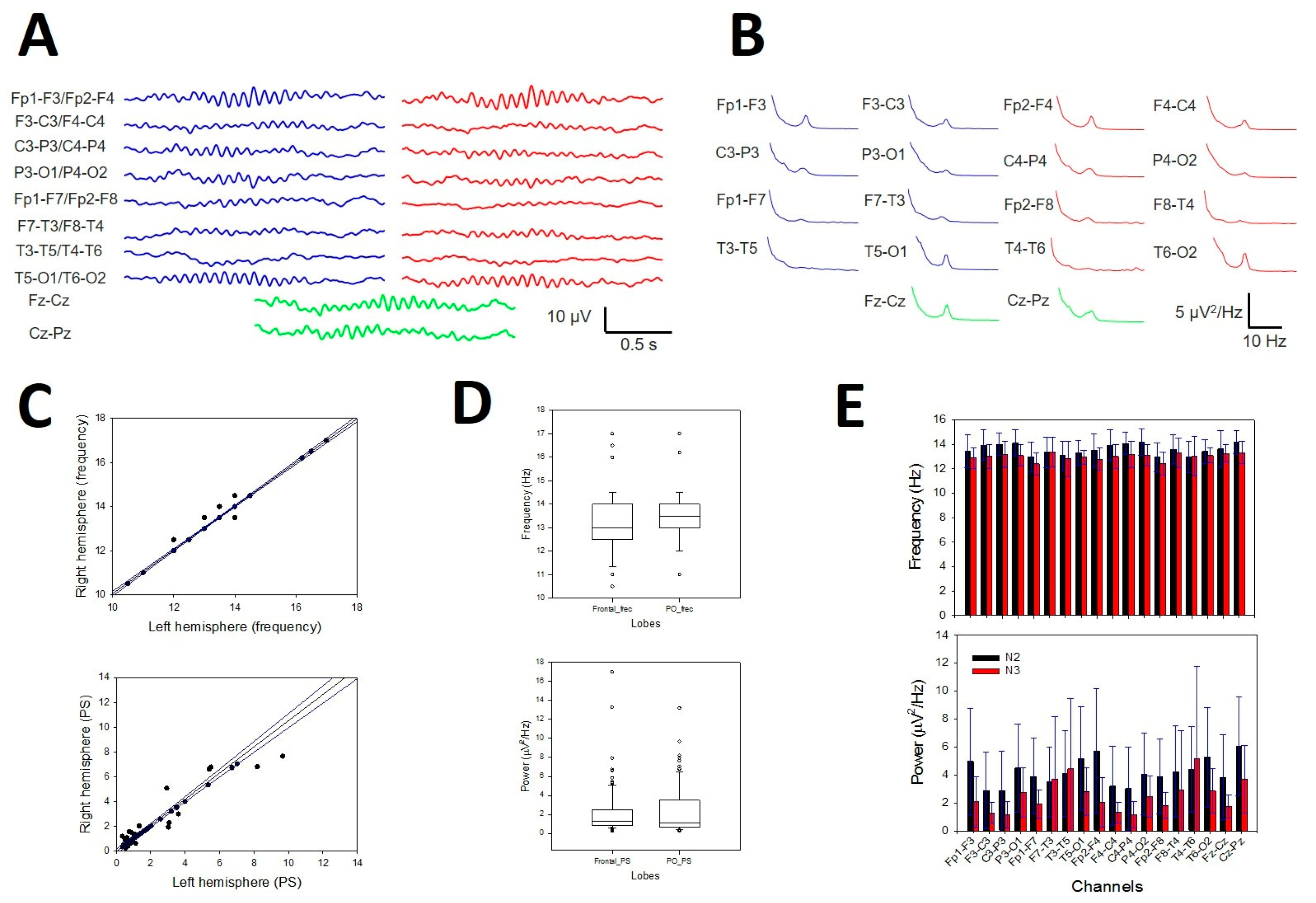
Sleep spindles were distributed across the entire scalp (Figure 10A), but in some channels, they were difficult to distinguish from the background. Nevertheless, the presence of SSs (i.e., the σ band) can be easily identified in the PS by a well-defined σ component at approximately 13 Hz (Figure 10B). These are the reasons why we choose to analyse their distribution and properties instead of measuring durations and amplitudes. We did not observe any difference in the symmetric channels between the right and left hemispheres for pF (Figure 11C, upper row) or mP (Figure 10C, lower row). The σ component was always present in the frontopolar region (Fp1-F3/Fp2-F4, 19/19 patients), followed by the occipital region (P3-O1/P4-O2 and T5-O1/T6-O2, 18/19), while the midtemporal areas presented a lower σ band (F7-T3/F8-T4 13/19 and T3-T5/T4-T6 12/19). We addressed the average value at the N2 sleep stage for pF and mP at the F, PO and T lobes (considering both hemispheres). We obtained a lower value (Med and 25–75 interpercentile range) for the F lobe (13.0, [12.5, 14.0] Hz and 1.05, [0.77, 1.62] µV2/Hz, respectively) and a higher value for the PO lobe (13.5, [13.0, 14.0] Hz and 1.07, [0.63, 3.47] µV2/Hz, respectively). The difference between the two regions was statistically significant for frequency (p = 0.020, for the Mann‒Whitney Rank sum test; for pF Figure 10D, upper row). No differences were observed regarding either the T lobe or the average mP (1.30, [0.83, 2.47] for F and 1.07 [0.63, 3.47] for PO, p = 0.566 for the Mann‒Whitney Rank sum test; see Figure 10D, lower row). Finally, we addressed the average pF and mP for the N2 and N3 sleep stages (Figure 10E). The frequency was statistically lower during the N3 stage than during the N2 stage (12.9 [12.7, 13.2] and 13.5 [13.3, 14.0] Hz, respectively, p < 0.001 for the Mann‒Whitney rank sum test), and a similar result was obtained for the average mP, which was lower for N3 than for N2 (2.5 ± 0.3 and 4.2 ± 0.2 µV2/Hz, respectively, p < 0.001 for the Student-t test).
Figure 10.
Numerical properties of SSs. A) Example of SSs from a patient. B) aPS for all the channels in the same patient. A prominent peak 13 Hz (σ band) is clearly observed in 14 graphs; blue lines = left hemisphere, red lines = right hemisphere and green lines = midline. C) Upper row. Linear regression ± 95% confidence band for the average frequency of symmetric channels in both hemispheres (r = 0.9961; p < 10-4, function ). Lower row. Linear regression ± 95% confidence band for the average power of symmetric channels of both hemispheres (r = 0.9924; p < 10-4, function ) D) Bar graph for the frequency (upper row) and the power for all the channels at the N2 and N3 sleep stages. Black = N2 stage, red = N3 stage. The error bars are the CIs.
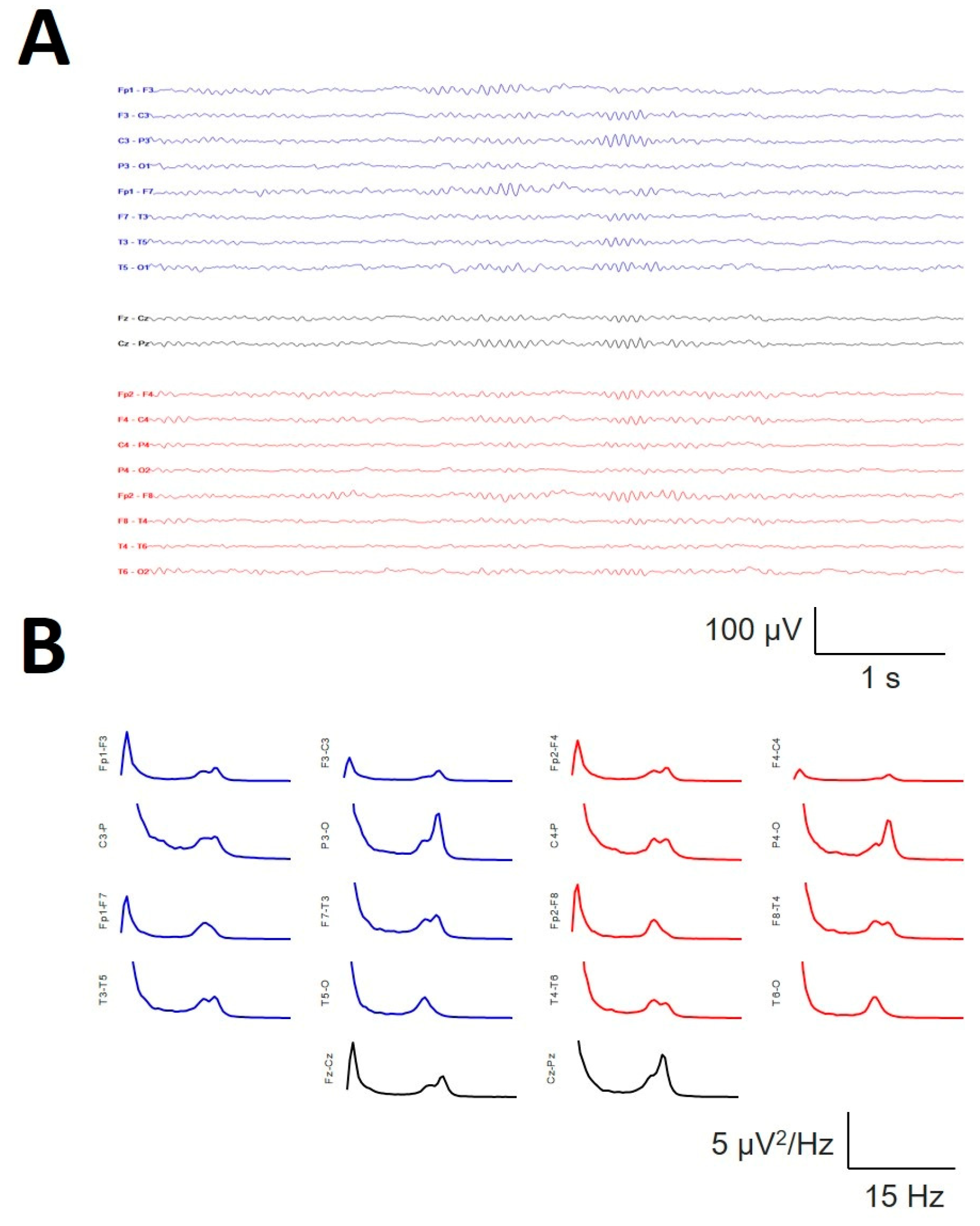
In a subset of 6/19 patients, the presence of the σ band of well-defined bimodal components during the N2 sleep stage was observed, as shown in Figure 11, where bimodal distributions at 12.5 and 14.5 Hz can be observed at several channels, e.g., Fp1-F3/Fp2-F4, F7-T3/F8-T4 or Fz-Cz. All of these bimodal σ components were obtained during the N2 sleep stage and therefore cannot be confused with the slow SS.
Figure 11.
Example of a bimodal σ band in the same patient during the N2 sleep stage. A) Raw trace showing the coexistence of SSs at two different frequencies (12.5 and 14.5 Hz). B) Average spectra for all the channels.
Figure 11.
Example of a bimodal σ band in the same patient during the N2 sleep stage. A) Raw trace showing the coexistence of SSs at two different frequencies (12.5 and 14.5 Hz). B) Average spectra for all the channels.
Finally, we addressed the relationship between the amplitude of the σ band and the density of SSs in a numerical simulation of the well-controlled percentage of SSs (Figure 12A). The average PS in the anterior regions showed an easily identifiable σ band (Figure 12B), from nearly zero (0% SSs) to a maximum when all the reconstructions included SSs (Figure 12A, lower row). The linear regression between the frontopolar (Figure 12C) and anterior midline channels (Figure 12D) was essentially one (r = 0.9964 and r = 0.9949, respectively). Therefore, there was a linear relationship between the density of SSs and the amplitude of the σ band in the anterior region.
4. Discussion
In this work, we revisited the spectral and synchronization properties of the wake and sleep stages for the whole scalp via double banana bipolar recordings in subjects without organic pathology. We have described these numerical properties for all electrodes of the international 10-20 system and not for the reduced number of electrodes commonly used in PSG studies. We have shown that both the structure for band composition and synchronization are highly complex and change throughout all phases of sleep. The numerical properties of KCs and SSs have also been described.
Usually, the PSG description of the sleep stages includes channels that do not acquire cerebral activity, such as EOG or EMG [5,10]. Although the brainstem and diencephalic structures that regulate the sleep stages project and modify the nuclei involved in muscle tone or eye movements, they do not receive feedback from the latter structures in a regulatory way. Therefore, all circadian states, from the awake state through different sleep stages, are products of the neural interactions of the brainstem, thalamus, hypothalamus and cortex; consequently, brain cortex activity is sufficient to define and differentiate all of these states [2,7,8]. This is a remarkable point because although EMGs or EOGs can be helpful for identifying different stages, they are not needed to stage sleep and wake, which are defined by EEG activity. In fact, previous studies have indicated that spectral analysis could serve as a method for sleep staging [22]. Although staging was not our goal, we have shown that the properties of the different phases of sleep and W are easy to identify and can be numerically described to implement these properties in automatic methods for sleep staging.
It has been shown that women present NREMS EEG spectra with higher absolute spectral densities than age-matched males [31,32]. Our data are not exactly the same. In fact, we did not find differences for N1 and N3 for the grand averages of logPS between men and women but for stages N3 and REM. Most likely, the different configurations of the EEG recordings (referential, instead of bipolar) and the widest coverage in our work, including all the IS 10-20 electrodes, could explain this discrepancy. Every EEG montage has pros and cons, and this is even more relevant for the qEEG. In fact, it was shown that a reference montage seriously biases the EEG power and coherence spectra, confounding the interpretation of the results [33]. Consequently, PS and logPS values can differ for referential and bipolar montages. Nevertheless, the global Coh for the whole band and all the scalps presented lower values for women at the W, N1 and N2 stages. No differences were observed between the sexes for ρ. However, considering not grand averages but topographical localizations, no statistically significant differences were observed between the sexes. This fact allowed us to group the values from males and females during topographical analysis.
Differences in average PS and synchronization throughout all phases of sleep and across spectra have been described [22]. Our results are partially superimposed on the previous results. We have shown that slow activity increased from W to N3, with a maximum for the entire scalp. A homogeneous state is characterized by a uniform structure or composition throughout. The most inhomogeneous state was W, where the F, PO and T lobes presented the greatest differences. However, homogeneity increased throughout sleep until the most homogeneous state was reached at N3. During the REM stage, inhomogeneity returned to the N1 level. Notably, no differences between the PO and T lobes were observed for any of the stages analysed. There is a significant similarity between the PO and T lobes in terms of the analytical method used. The differences between the definite lobes and phases were also remarkable. These differences were greater for F lobes, where all the combinations, including the δ band, were different from the rest of the bands, followed by PO and finally T. The δ band was obviously the most variable across the dynamics of wake–sleep. In contrast, the less different pair of bands was α/β, which was significant mainly for the F lobe (60% of cases), and nothing at all for the T lobe.
Coherence between two channels is the ratio between the square of the absolute value of the cross-spectrum and the average autospectra of both [22,24] used a measure that included only the numerator. Consequently, considering that the measurements were performed mainly between hemispheres, their measurements obviously cannot be similar to ours. Considering the band coherence for all the stages, we have shown that there is a difference between N3 and the W, N1 and REM stages but not between N2 and any other stage. The Coh of the β band was quite similar for all the phases. No difference between δ and θ coherence was observed for any phase, but all the stages showed a difference between the δ/α and δ/β θ/α pairs. The β band showed the lowest global coherence for all the phases. The analysis of the coherence structure for all the N2 phases revealed the greatest difference between the lobes. The most homogeneous phase was W, although differences between F and PO and PO and T lobes were observed for the β band. The pairs of significant differences followed the same order observed for logPS. Globally considered, all the phases presented the lowest values of all the bands for the PO lobes and, systematically, for the β band. Regarding differences between bands measured at the same stage and lobe, it is clear that the lower differences are for T lobes, probably because the dispersion is greater in this region, biasing the statistical significance.
Although they share some common features, the structures of logPS and Coh clearly differ from phase to phase, indicating that both properties are independent across the different stages of sleep.
The variable ρ is also a measure of linear synchronization widely used in qEEG in the voltage domain [34,35]. The structure of the synchronization determined by ρ was different from that determined by means of coherence. Globally, the structure of ρ across the phases reflects coherence for bands δ to α but not β. The scalp structure for every stage is also similar to the structure of the different bands of coherence, with a minimum value for PO lobes and a greater dispersion at T lobes. In terms of coherence, the W stage exhibited the most homogenous state.
The grand average PS reveals great differences between the different phases of sleep through the scalp. Obviously, the presence of the alpha band at 10 Hz was notoriously observed in posterior regions during W. This component slowed down and moved to anterior regions during N1. During all the phases of sleep, in both NREM and REM sleep, a slower alpha component was easily observed at approximately 8 H [22].
The maximum amplitude of KCs has sometimes been described at the vertex [6], although the majority of authors have described the maximum amplitude at the prefrontal and frontal regions [36,37]. This distribution is in good agreement with our results, where we observed a more frontal location, with the maximum at F3-C3/F4-C4, and even more anterior at frontopolar temporal sides (Fp1-F7/Fp2-F8). This lateral maximum for KCs was not previously described because most of the articles use a reduced number of electrodes instead of the 10-20 completed system used here. Some authors reported extremely variable morphology [38,39]; however, we obtained highly robust morphology across the subjects, except for the fronto-polar channels Fp1-F3/Fp2-F4, which showed great variability. In fact, we have not only observed a systematic anterior‒posterior gradient for amplitude but also observed in the case of the duration with the maximum duration in the lateral fronto-polar regions (nearly 1 second duration) and the shortest duration in the temporo‒occipital regions (below the 0.5 second duration of the KC definition). Therefore, although KCs can be recorded through the scalp, it has a nonuniform amplitude and duration; in contrast, the anterior regions have the highest and longest waveforms, whereas in the occipital regions, the amplitude and duration are lower.
The definition of the AASM for an SS in an adult human is that of a “train of distinct waves with frequency 11–16 Hz (most commonly 12–14 Hz) with a duration ≥ 0.5 s, usually maximal in amplitude using central derivations [10]. The reliability of visual detection between experts is generally considered to be >80% and improves further once the number of included expert scorers increases [40]. The intraspindle frequency reported is 13.3 ± 1 Hz [41,42]. We observed a Gaussian distribution with a value of 13.4 ± 1.2, which fits well with these previously published values.
SS dynamics and quantity can be measured by the mean power values in the σ band [41], and this has been the approach followed in this work. Two types of SSs (i.e., the σ band) have been described, depending on the sleep phase. During the N2 stage, the faster σ component is prominent, with a pF ≥ 12.5 Hz; meanwhile, during the N3 stage, a slower component can be observed, with a pF < 12.5 Hz [43,44,45]. We observed this fact, with a σ component at 13 Hz for N2 and a slower component at approximately 12 Hz during N3. However, we are not aware of previous reports showing the presence of bimodal components of the sigma band in the same state. We observed the presence of SSs and σ components at two frequencies during the N2 phase. We excluded the mixture of N2+N3 sleep stages because of the relatively small component of the delta band in the PS.
We have not addressed the different scalp locations for slow and fast SSs, although differences between the two types of SSs have been described [45,46,47]. However, we identified a pattern with two maxima in the fronto-polar and occipital regions. Surprisingly, the average pF at fronto-polar regions was slower than that at the occipital lobe, which has not been previously described. This difference in pF was not associated with differences in mP. Therefore, if, as we argue, mP is an estimate of spindle density (see below), this implies that spindle density was not modified along the fronto-occipital axis, although pF was.
Finally, the SSs are related to the macrostructure of sleep and the underlying oscillation associated with 0.02 Hz, defining phases of continuity and fragility of sleep [41,48,49,50]. Alterations in SS regulation can be associated with changes in microstates, such as cyclic alternating periods, which are associated with periodic leg movements or bruxism [51], or even with pathologies, such as Alzheimer’s disease [52,53]. The magnitude of the σ band can be an easy and straightforward way to estimate the density and mean frequency of SSs and could be useful in sleep medicine.
In summary, we have comprehensively and deeply described the properties of PS and synchronization structures in humans without pathology, which is the most common recording method for EEG and video-EEG recordings in clinical practice [24]. The clear definition of normative values is the first step in identifying sleep pathologies. We are aware that the number of subjects is not too high; however, the results obtained, such as the PS, as the synchronization of logPS values, have been very robust. Another limitation is that these subjects were not healthy volunteers; in fact, some of them experienced psychological alterations, although not pathologies such as epilepsy or other structural illnesses. However, these situations, as well as the first-night effect, are more related to alterations in the hypnogram, which has not been estimated, than to the spectral or synchronization properties of the sleep states.
5. Conclusions
The spectral and synchronization structure is very complex and evolves throughout the different phases of sleep, although not necessarily in parallel. The average power spectra have been found to be highly specific for each of the sleep phases and could therefore be used (or band values) as a simple and reliable method for sleep staging. The high specificity of the spectral patterns of the different phases makes the use of accessory channels for sleep staging, such as EMG or EOG, unnecessary, as the difference between them is sufficiently clear.
We have observed that the distribution of KCs has a more peripheral distribution than assumed, with a well-defined anterior‒posterior gradient. SSs have fronto-polar and occipital maxima but with differences in the average frequency, which is lower in the frontal region. Another fact not previously described is the presence of bimodal spindles in a percentage of the subjects. Finally, we observed that sigma band amplitude correlates very well with spindle density, so this method could easily be used for the study of sleep pathologies.
Author Contributions
JP was responsible for the idea. PGZ and JP participated in data collection. JP developed the analytical methods; PGZ and LV-Z participated in analysis and interpretation and JP was responsible for manuscript preparation. All authors approved the submitted version of this manuscript.
Funding
this work was financed by a grant from the Instituto de Salud Carlos III (ISCIII) PI23/00393 and was partially supported by FEDER (Fonds Europeen de Development Economique et Regional).
Institutional Review Board Statement
The experimental procedure was approved by the medical ethical review board of the Hospital Universitario de La Princesa (ref 5548).
Informed Consent Statement
Patient consent was waived due to was deemed “care as usual”.
Conflicts of Interest
The authors declare no conflict of interest.
Abbreviations
| aKC | average K-complex. |
| aPS | average power-spectrum. |
| CI | confidence interval. |
| Coh | coherence. |
| EEG | electroencephalography. |
| ECG | electrocardiography. |
| EMG | electromyography. |
| EOG | electrooculogram. |
| F | frontal. |
| FFT | fast Fourier transform. |
| H | hemispheric. |
| KC | K-complexes. |
| logPS | logarithm transform of PS. |
| maxΔh | absolute difference between all the aPS for every channel. |
| mP | maximum power. |
| N1 | NREM stage 1. |
| N2 | NREM stage 2. |
| N3 | NREM stage 3. |
| NREM | non-rapid eye movement sleep state. |
| pF | peak frequency. |
| PO | parieto-occipital. |
| PSG | polysomnography. |
| REM | rapid eye movement sleep state. |
| rsEEG | resting-state EEG. |
| SS | sleep spindles. |
| SSE | Shannon’s spectral entropy. |
| T | temporal. |
| vEEG | video-electroencephalography. |
| VSW | vertex sharp waves. |
| α | alpha band. |
| β | beta band. |
| δ | delta band. |
| θ | theta band. |
| ρ | Pearson’s correlation coefficient. |
| σ | sigma band. |
Appendix A
Figure A1.
Analysis of typical waveforms of sleep. A). SS and B). K-complex.
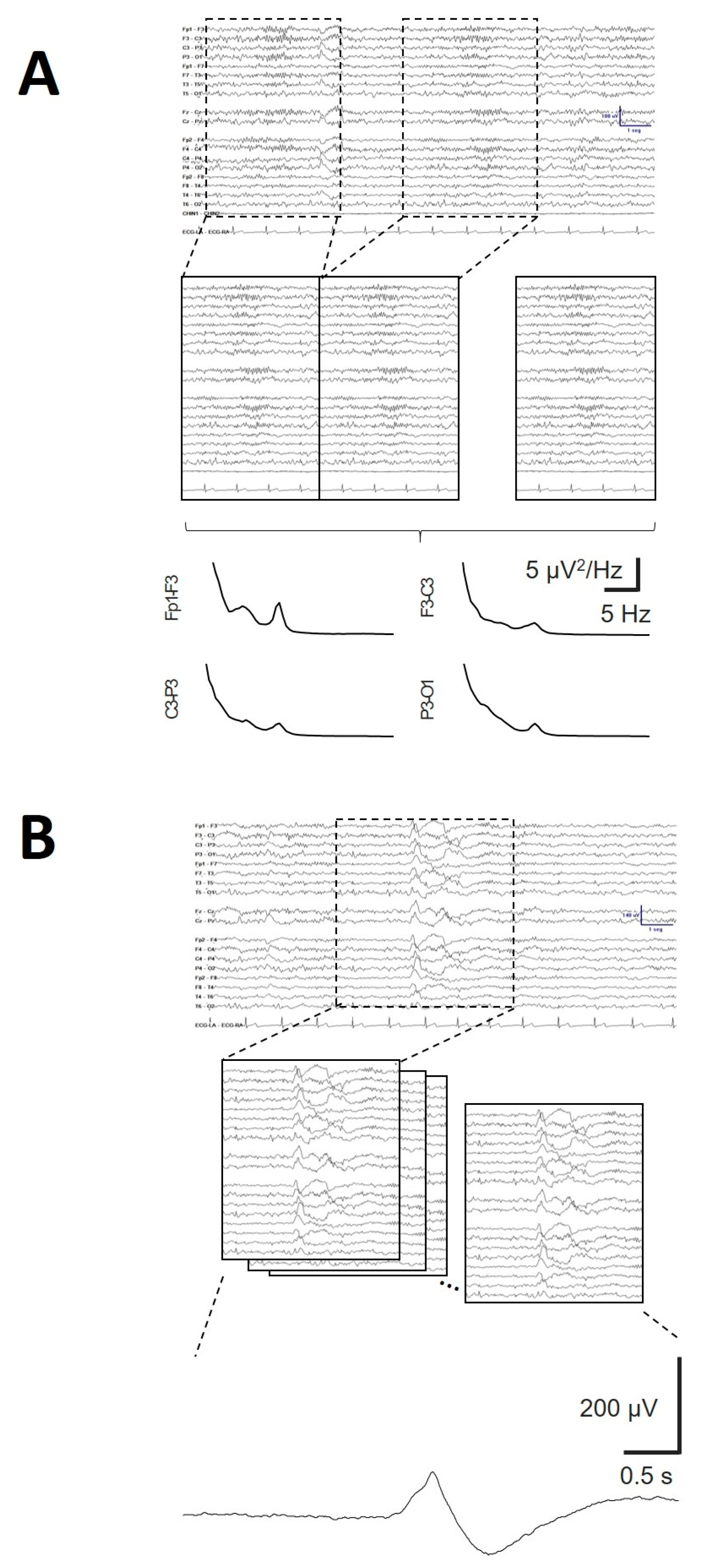
Figure A2.
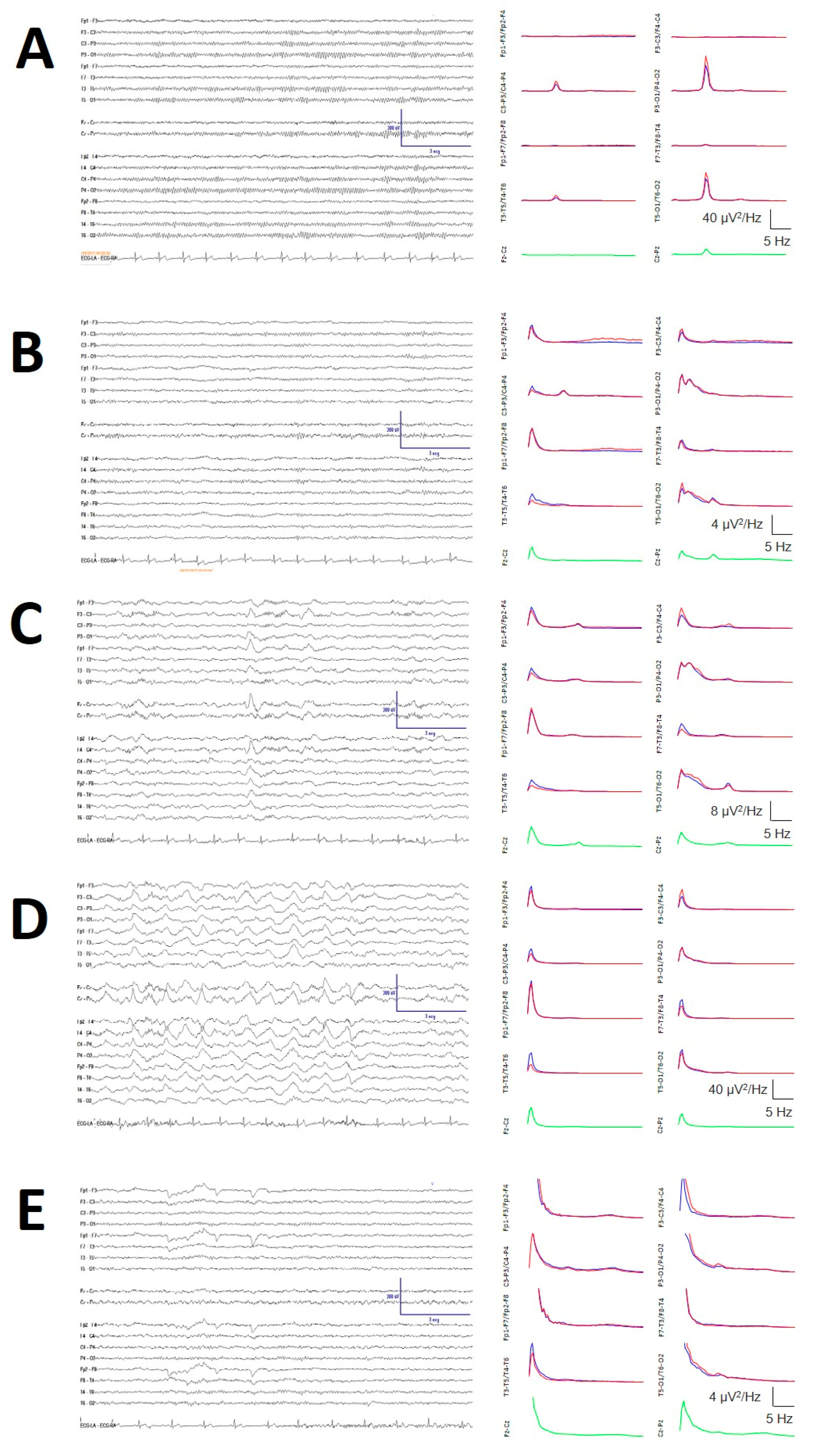
Sleep staging. The left column shows the bipolar raw traces, and the right column shows the mean PS for channels (indicated at y-labels) for the left (blue), right (red) and sagittal channels (green). A) Wake stage, showing a prominent occipital alpha component at 10 Hz. B) N1 stage, with a slower occipital component and an increase in the delta frequency. C) N2 stage with the presence of SSs and KCs in the left column and a high-amplitude delta component and a small 14 Hz component, indicating the presence of SSs. D) N3 stage: the highest delta component (note the y-axis calibration). E) REM stage, clearly visible by the presence of vertical and horizontal eye movements with a slower 8.5 Hz alpha component and absence of an SS component.
Figure A2.
Sleep staging. The left column shows the bipolar raw traces, and the right column shows the mean PS for channels (indicated at y-labels) for the left (blue), right (red) and sagittal channels (green). A) Wake stage, showing a prominent occipital alpha component at 10 Hz. B) N1 stage, with a slower occipital component and an increase in the delta frequency. C) N2 stage with the presence of SSs and KCs in the left column and a high-amplitude delta component and a small 14 Hz component, indicating the presence of SSs. D) N3 stage: the highest delta component (note the y-axis calibration). E) REM stage, clearly visible by the presence of vertical and horizontal eye movements with a slower 8.5 Hz alpha component and absence of an SS component.
Appendix B

Table A1.
Average logPS by lobes and different phases of wake and sleep comparing left and right sides. Neither of the paired lobes resulted different for any sleep phase.
Table A1.
Average logPS by lobes and different phases of wake and sleep comparing left and right sides. Neither of the paired lobes resulted different for any sleep phase.
| Band | Lobe | W | N1 | N2 | N3 | REM | |||||
|---|---|---|---|---|---|---|---|---|---|---|---|
| Delta | lF | 4.34 | ±0.18 | 2.73 | ±0.35 | 2.46 | ±0.19 | 2.85 | ±0.19 | 3.27 | ±0.11 |
| rF | 4.32 | ±0.20 | 2.72 | ±0.40 | 2.49 | ±0.19 | 2.84 | ±0.20 | 3.30 | ±0.12 | |
| lPO | 4.37 | ±0.21 | 2.70 | ±0.29 | 2.58 | ±0.22 | 2.72 | ±0.23 | 3.32 | ±0.19 | |
| rPO | 3.70 | ±0.22 | 2.43 | ±0.29 | 2.37 | ±0.22 | 2.58 | ±0.24 | 3.02 | ±0.19 | |
| lT | 4.63 | ±0.24 | 3.00 | ±0.34 | 2.88 | ±0.30 | 3.09 | ±0.27 | 3.53 | ±0.22 | |
| rT | 3.84 | ±0.24 | 2.75 | ±0.33 | 2.70 | ±0.30 | 2.72 | ±0.27 | 3.11 | ±0.22 | |
| Theta | lF | 2.19 | ±0.02 | 1.29 | ±0.19 | 1.36 | ±0.02 | 1.35 | ±0.02 | 1.78 | ±0.02 |
| rF | 2.04 | ±0.19 | 1.30 | ±0.19 | 1.47 | ±0.16 | 1.39 | ±0.16 | 1.70 | ±0.14 | |
| lPO | 2.46 | ±0.17 | 1.64 | ±0.23 | 1.89 | ±0.16 | 1.69 | ±0.16 | 2.12 | ±0.14 | |
| rPO | 2.70 | ±0.24 | 1.93 | ±0.34 | 2.41 | ±0.18 | 2.02 | ±0.18 | 2.35 | ±0.16 | |
| lT | 2.56 | ±0.23 | 1.73 | ±0.29 | 1.95 | ±0.17 | 1.87 | ±0.18 | 2.22 | ±0.17 | |
| rT | 2.56 | ±0.26 | 1.73 | ±0.29 | 1.95 | ±0.23 | 1.87 | ±0.22 | 2.22 | ±0.22 | |
| Alpha | lF | 1.62 | ±0.02 | ±0.71 | ±0.22 | 1.39 | ±0.02 | 1.06 | ±0.02 | 1.32 | ±0.02 |
| rF | 1.64 | ±0.19 | ±0.69 | ±0.21 | 1.42 | ±0.14 | 1.09 | ±0.14 | 1.35 | ±0.14 | |
| lPO | 1.90 | ±0.17 | 1.37 | ±0.29 | 2.51 | ±0.13 | 1.70 | ±0.14 | 1.68 | ±0.13 | |
| rPO | 1.94 | ±0.27 | 1.40 | ±0.30 | 2.52 | ±0.16 | 1.73 | ±0.17 | 1.71 | ±0.17 | |
| lT | 1.94 | ±0.27 | 1.36 | ±0.33 | 2.31 | ±0.15 | 1.73 | ±0.18 | 1.78 | ±0.17 | |
| rT | 1.94 | ±0.24 | 1.36 | ±0.33 | 2.31 | ±0.23 | 1.73 | ±0.24 | 1.78 | ±0.22 | |
| Beta | lF | 1.17 | ±0.03 | ±0.99 | ±0.17 | 1.26 | ±0.02 | 1.24 | ±0.01 | 1.07 | ±0.02 |
| rF | 1.14 | ±0.17 | 1.07 | ±0.19 | 1.38 | ±0.13 | 1.39 | ±0.15 | 1.17 | ±0.12 | |
| lPO | 1.22 | ±0.18 | 1.14 | ±0.20 | 1.73 | ±0.14 | 1.38 | ±0.14 | 1.27 | ±0.13 | |
| rPO | 1.25 | ±0.18 | 1.21 | ±0.22 | 1.74 | ±0.16 | 1.45 | ±0.17 | 1.36 | ±0.15 | |
| lT | 1.38 | ±0.19 | 1.24 | ±0.26 | 1.89 | ±0.17 | 1.59 | ±0.18 | 1.42 | ±0.16 | |
| rT | 1.38 | ±0.16 | 1.24 | ±0.26 | 1.89 | ±0.21 | 1.59 | ±0.22 | 1.42 | ±0.20 | |
| SSE | lF | 3.29 | ±0.02 | 3.93 | ±0.33 | 4.01 | ±0.01 | 3.91 | ±0.01 | 3.75 | ±0.01 |
| rF | 3.30 | ±0.09 | 3.96 | ±0.33 | 4.07 | ±0.07 | 4.00 | ±0.06 | 3.77 | ±0.06 | |
| lPO | 3.30 | ±0.08 | 4.04 | ±0.33 | 3.99 | ±0.08 | 4.05 | ±0.07 | 3.85 | ±0.06 | |
| rPO | 3.33 | ±0.09 | 4.04 | ±0.33 | 3.96 | ±0.07 | 4.05 | ±0.07 | 3.86 | ±0.05 | |
| lT | 3.23 | ±0.08 | 3.96 | ±0.33 | 4.11 | ±0.07 | 4.01 | ±0.07 | 3.83 | ±0.05 | |
| rT | 3.23 | ±0.10 | 3.96 | ±0.33 | 4.11 | ±0.08 | 4.01 | ±0.07 | 3.83 | ±0.05 | |
lF = left frontal; rF = right frontal; lPO = left parieto-occipital; rPO = right parieto-occipital; lT= left temporal; rT = right temporal.
References
- Pace-Schott, E.F. Sleep architecture. In The Neuroscience of Sleep; Stickgold, R., Walker, M.P., Eds.; Academic Press: London, UK, 2009; pp. 11–17. ISBN 9780123750730. [Google Scholar]
- Rechtschaffen, A.; Siegel, J.M. Sleep and Dreaming. In Principles of Neuroscience, 4th ed.; Kandel, E.R., Schwartz, J.H., Jessel, T.M., Eds.; McGraw-Hill: New York, 2000; pp. 936–947. [Google Scholar]
- Steriade, M.; Nunez, A.; Amzica, F.A. Novel slow (<1 Hz) oscillation of neocortical neurons in vivo: depolarizing and hyperpolarizing components. J Neurosci 1993, 13, 3252–3265. [Google Scholar] [CrossRef]
- Steriade, M.; Contreras, D.; Dossi, R.C.; Nunez, A. The slow (<1 Hz) oscillation in reticular thalamic and thalamocortical neurons: scenario of sleep rhythm generation in interacting thalamic and neocortical networks. J Neurosci 1993, 13, 3284–3299. [Google Scholar] [CrossRef]
- Rama, A.N.; Cho, S.C.; Kushida, C.A. Normal Human Sleep. In Sleep: a comprehensive handboock; Lee-Chiong, T., Ed.; John Wiley and Son, 2006; pp. 3–10. ISBN 978-0-471-68371-1. [Google Scholar]
- Shneerson, J.M. Sleep medicine: a guide to sleep and its disorders, 2nd ed.; Blackwell Publishing Ltd.: Oxford OX4 2DQ, UK, 2005; ISBN 978-1-4051-2393-8. [Google Scholar]
- Carskado, W.C.; Dement, M.A. Normal human sleep an overview. In Principles and practice of sleep medicine, 5th ed.; Kryger, M.H., Roht, T., Dement, W.C., Eds.; Elsevier, 2011. [Google Scholar]
- McCormick, D.A. Sleep and Wakefulness. In Neuroscience, 3rd ed.; Purves, D., Augustine, G.J., Fitzpatrick, D., Hall, W.C., LaMantia, A.S., McNamara, J.O., Williams, S.M., Eds.; Sinauer Associates: Massachusetts, USA, 2004; ISBN 0-87893-725-0. [Google Scholar]
- Kryger, M.H.; Roth, T.; Dement, W.C. Principles and practice of sleep medicine, 5th ed.; Kryger, M.H., Roth, T., Dement, W.C., Eds.; Elsevier: St. Louis, 2011; ISBN 978-1-4160-6645-3. [Google Scholar]
- American Academy of Sleep Medicine. AASM Manual for the Scoring of Sleep and Associated Events: Rules, Terminology and Technical Specifications (Version 3). 2023. [Google Scholar]
- Oliveir, G.H.B.S.; Coutinho, L.R.; da Silva, J.C.; Pinto, I.J.P.; Ferreira, J.M.S.; Silva, F.J.S.; Pinto, I.J.P.; Ferreira, J.M.S.; Silva, F.J.S.; Santos, D.V.; Teles, A.S. Multitaper-based method for automatic k-complex detection in human sleep EEG. Expert Syst Appl 2020, 151, 113331. [Google Scholar] [CrossRef]
- Camilleri, T.A.; Camilleri, K.P.; Simon, G.; Fabri, S.G. Automatic detection of spindles and K-complexes in sleep EEG using switching multiple models. Biomedical Signal Processing and Control 2014, 117–127. [Google Scholar] [CrossRef]
- Perumalsamy, V.; Sankaranarayanan, S.; Rajamony, S. Sleep spindles detection from human sleep EEG signals using autoregressive (AR) model: a surrogate data approach. J Biomed Sci Eng 2009, 02, 294–303. [Google Scholar] [CrossRef]
- Ogilvie, R.D.; Simons, I.A.; Kuderian, R.H.; Macdonald, T.; Rustenburg, J. Behavioral. event-related potential and EEG/FFT changes at sleep onset. Psychophysiology 1991, 28, 54–64. [Google Scholar] [CrossRef] [PubMed]
- Hadjiyannakis, K.; Ogilvie, R.D.; Alloway, C.E.D.; Shapiro, C. FFT analysis of EEG during stage 2-to-REM transitions in narcoleptic patients and normal sleepers. Electroen Clin Neuro 1997, 103, 543–553. [Google Scholar] [CrossRef]
- Krishnan, P.; Yaacob, S.; Krishnan, A.P.; Rizon, M.; Ang, C.K. EEG based drowsiness detection using relative band power and short-time Fourier transform. J Robot Netw Artif L 2020, 7, 147–151. [Google Scholar] [CrossRef]
- Kang, J.M.; Cho, S.E.; Na, K.S.; Kang, S.G. Spectral power analysis of sleep electroencephalography in subjects with different severities of obstructive sleep apnea and healthy controls. Nat Sci Sleep 2021, 13, 477–486. [Google Scholar] [CrossRef] [PubMed]
- Aydin, S.; Tunga, M.A.; Yetkin, S. Mutual information analysis of sleep EEG in detecting psycho-physiological insomnia. J Med Syst 2015, 39, 43. [Google Scholar] [CrossRef] [PubMed]
- Bajaj, V.; Pachori, R.B. Automatic classification of sleep stages based on the time-frequency image of EEG signals. Comput Meth Prog Bio 2013, 112, 320–328. [Google Scholar] [CrossRef] [PubMed]
- Huang, H.; Zhang, J.; Zhu, L.; Tang, J.; Lin, G.; Kong, W.; Lei, X.; Zhu, L. EEG-Based Sleep Staging Analysis with Functional Connectivity. Sensors 2021, 21, 1988. [Google Scholar] [CrossRef] [PubMed]
- Johnson, L.; Lubin, A.; Naitoh, P.; Nute, C.; Austin, M. Spectral analysis of the EEG of dominant and non-dominant alpha subjects during waking and sleeping. Electroencephalogr Clin Neurophysiol 1969, 26, 361–337. [Google Scholar] [CrossRef]
- Dumermuth, G.; Lange, B.; Lehmann, D.; Meier, C.A.; Dinkelmann, R.; Molinari, L. Spectral analysis of all-night sleep EEG in healthy adults. Eur Neurol 1983, 22, 322–339. [Google Scholar] [CrossRef]
- Cortés, D.; Vega-Zelaya, L.; Lopez, L.; Toledo, M.; Pastor, J. Utility of video-electroencephalography monitoring for diagnosis of epilepsy and non-epileptic paroxysmal events. Archives of Women Health and Care 2020, 3, 1–6. [Google Scholar]
- Pastor, J.; Vega-Zelaya, L. Normative Structure of Resting-State EEG in Bipolar Derivations for Daily Clinical Practice: A Pilot Study. Brain Sci 2023, 13, 167. [Google Scholar] [CrossRef]
- Vega-Zelaya, L.; Martín Abad, E.; Pastor, J. Quantified EEG for the characterization of epileptic seizures versus periodic activity in critically ill patients. Brain Sci 2020, 10, 158. [Google Scholar] [CrossRef] [PubMed]
- Pastor, J.; Vega-Zelaya, L.; Martin Abad, E. Specific EEG encephalopathic pattern in SARS-CoV-2 patients. J. Clin. Med. 2020, 9, 1545. [Google Scholar] [CrossRef]
- Ruchkin, D. EEG coherence. Int J Psychophysiol 2005, 57, 83–85. [Google Scholar] [CrossRef]
- Coben, R.; Clarke, A.R.; Hudspeth, W.; Barry, R.J. EEG power and coherence in autistic spectrum disorder. Clin Neurophysiol 2008, 119, 1002–1009. [Google Scholar] [CrossRef]
- Smulders, F.T.Y.; ten Oever, S.; Donkers, F.C.L.; Quaedflieg, C.W.E.M.; van de Ven, V. Single-trial log transformation is optimal in frequency analysis of resting EEG alpha. Eur J Neurosci 2018, 48, 2585–2598. [Google Scholar] [CrossRef]
- Spiegel, M.R. Teoría de la correlación. In Spiegel MR: Estadística Madrid; McGraw-Hill Interamericana: Madrid, 1991; pp. 322–356. [Google Scholar]
- Carrier, J.; Land, S.; Buysse, D.J.; Kupfer, D.J.; Monk, T.H. The effects of age and gender on sleep EEG power spectral density in the middle years of life (ages 20-60 years old). Psychophysiology 2001, 38, 232–242. [Google Scholar] [CrossRef] [PubMed]
- Dijk, D.J.; Beersma, D.G.; van den Hoofdakker, R.H. All night spectral analysis of EEG sleep in young adult and middle-aged male subjects. Neurobiol Aging 1989, 10, 677–682. [Google Scholar] [CrossRef] [PubMed]
- Yao, D. A method to standardize a reference of scalp EEG recordings to a point at infinity. Physiol. Meas. 2001, 22, 693–711. [Google Scholar] [CrossRef] [PubMed]
- Ortega, G.J.; Menéndez de la Prida, L.; Sola, R.G.; Pastor, J. Synchronization clusters of interictal activity in the lateral temporal cortex of epileptic patients: intracranial analysis. Epilepsia 2008, 49, 269–280. [Google Scholar] [CrossRef]
- Palmigiano, A.; Pastor, J.; García de Sola, R.; Ortega, G.J. Stability of synchronization clusters and seizurability in temporal lobe epilepsy. PLoS One 2012, 7, e41799. [Google Scholar] [CrossRef] [PubMed] [PubMed Central]
- McCormic, L.; Nielsen, T.; Nicolas, A.; Ptito, M.; Montplaisir, J. Topographical distribution of spindles and K-complexes in normal subjects. Sleep 1997, 20, 939–941. [Google Scholar] [CrossRef] [PubMed]
- Colrain, I.M. The K-complex: a 7-decade history. Sleep 2005, 28, 255–273. [Google Scholar] [CrossRef] [PubMed]
- Ujszàszi, J.; Halász, P. Late component variants of single auditory evoked responses during NREM sleep stage 2 in man. Electroencephalogr Clin Neurophysiol 1986, 64, 260–268. [Google Scholar] [CrossRef]
- Da Rosa, A.C.; Kemp, B.; Paiva, T.; Lopes da Silva, F.H.; Mamphuisen, H.A. A model-based detector of vertex vawes and K complex in sleep electroencephalogram. Electroencephalogr Clin Neurophysiol 1991, 78, 71–79. [Google Scholar] [CrossRef]
- Wendt, S.L.; Welinder, P.; Sorensen, H.B.; Peppard, P.E.; Jennum, P.; Perona, P.; Mignot, E.; Warby, S.C. Inter-expert and intra-expert reliability in sleep spindle scoring. Clin Neurophysiol 2015, 126, 1548–1556. [Google Scholar] [CrossRef]
- Fernandez, L.M.J.; Lüthi, A. Sleep spindles: mechanisms and functions. Physiol Rev 2020, 100, 805–868. [Google Scholar] [CrossRef]
- Warby, S.C.; Wendt, S.L.; Welinder, P.; Munk, E.G.; Carrillo, O.; Sorensen, H.B.; Jennum, P.; Peppard, P.E.; Perona, P.; Mignot, E. Sleep-spindle detection: crowdsourcing and evaluating performance of experts, non-experts and automated methods. Nat Methods 2014, 11, 385–392. [Google Scholar] [CrossRef]
- De Gennaro, L.; Ferrara, M.; Vecchio, F.; Curcio, G.; Bertini, M. An electroencephalographic fingerprint of human sleep. Neuroimage 2005, 26, 114–122. [Google Scholar] [CrossRef] [PubMed]
- Mölle, M.; Bergmann, T.O.; Marshall, L.; Born, J. Fast and slow spindles during the sleep slow oscillation: disparate coalescence and engagement in memory processing. Sleep 2011, 34, 1411–1421. [Google Scholar] [CrossRef] [PubMed] [PubMed Central]
- Cox, R.; Schapiro, A.C.; Manoach, D.S.; Stickgold, R. Individual differences in frequency and topography of slow and fast sleep spindles. Front Hum Neurosci 2017, 11, 433. [Google Scholar] [CrossRef]
- De Gennaro, L.; Ferrara, M. Sleep spindles: an overview. Sleep Med Rev 2003, 7, 423–440. [Google Scholar] [CrossRef] [PubMed]
- Nakamura, M.; Uchida, S.; Maehara, T.; Kawai, K.; Hirai, N.; Nakabayashi, T.; Arakaki, H.; Okubo, Y.; Nishikawa, T.; Shimizu, H. Sleep spindles in human prefrontal cortex: an electrocorticographic study. Neurosci Res 2003, 45, 419–427. [Google Scholar] [CrossRef]
- Ehrhart, J.; Ehrhart, M.; Muzet, A.; Schieber, J.P.; Naitoh, P. K-complexes and sleep spindles before transient activation during sleep. Sleep 1981, 4, 400–407. [Google Scholar] [PubMed]
- Naitoh, P.; Antony-Baas, V.; Muzet, A.; Ehrhart, J. Dynamic relation of sleep spindles and K-complexes to spontaneous phasic arousal in sleeping human subjects. Sleep 1982, 5, 58–72. [Google Scholar] [CrossRef] [PubMed]
- Cardis, R.; Lecci, S.; Lüthi, A. The 0.02 Hz-oscillation in sigma power times spontaneous transitions from non-REM sleep. J Sleep Res 2018, 27, 226. [Google Scholar] [CrossRef]
- Manconi, M.; Silvani, A.; Ferri, R. Commentary: Coordinated infraslow neural and cardiac oscillations mark fragility and offline periods in mammalian sleep. Front Physiol 2017, 8, 847. [Google Scholar] [CrossRef] [PubMed] [PubMed Central]
- Gorgoni, M.; Lauri, G.; Truglia, I.; Cordone, S.; Sarasso, S.; Scarpelli, S.; Mangiaruga, A.; D’Atri, A.; Tempesta, D.; Ferrara, M.; Marra, C.; Rossini, P.M.; De Gennaro, L. Parietal fast sleep spindle density decrease in Alzheimer’s disease and amnesic mild cognitive impairment. Neural Plast 2016, 2016, 8376108. [Google Scholar] [CrossRef] [PubMed]
- Rauchs, G.; Schabus, M.; Parapatics, S.; Bertran, F.; Clochon, P.; Hot, P.; Denise, P.; Desgranges, B.; Eustache, F.; Gruber, G.; Anderer, P. Is there a link between sleep changes and memory in Alzheimer’s disease? Neuroreport 2008, 19, 1159–1162. [Google Scholar] [CrossRef] [PubMed]
Figure 1.
Typical waveforms of sleep. A) Average K-complex (aKC) and B) average PS showing the SS component. V1 = amplitude of the first component, d1 = duration of the first component; V2 = amplitude of the second component, d2 = duration of the second component; mP = maximum power; pF = peak frequency.
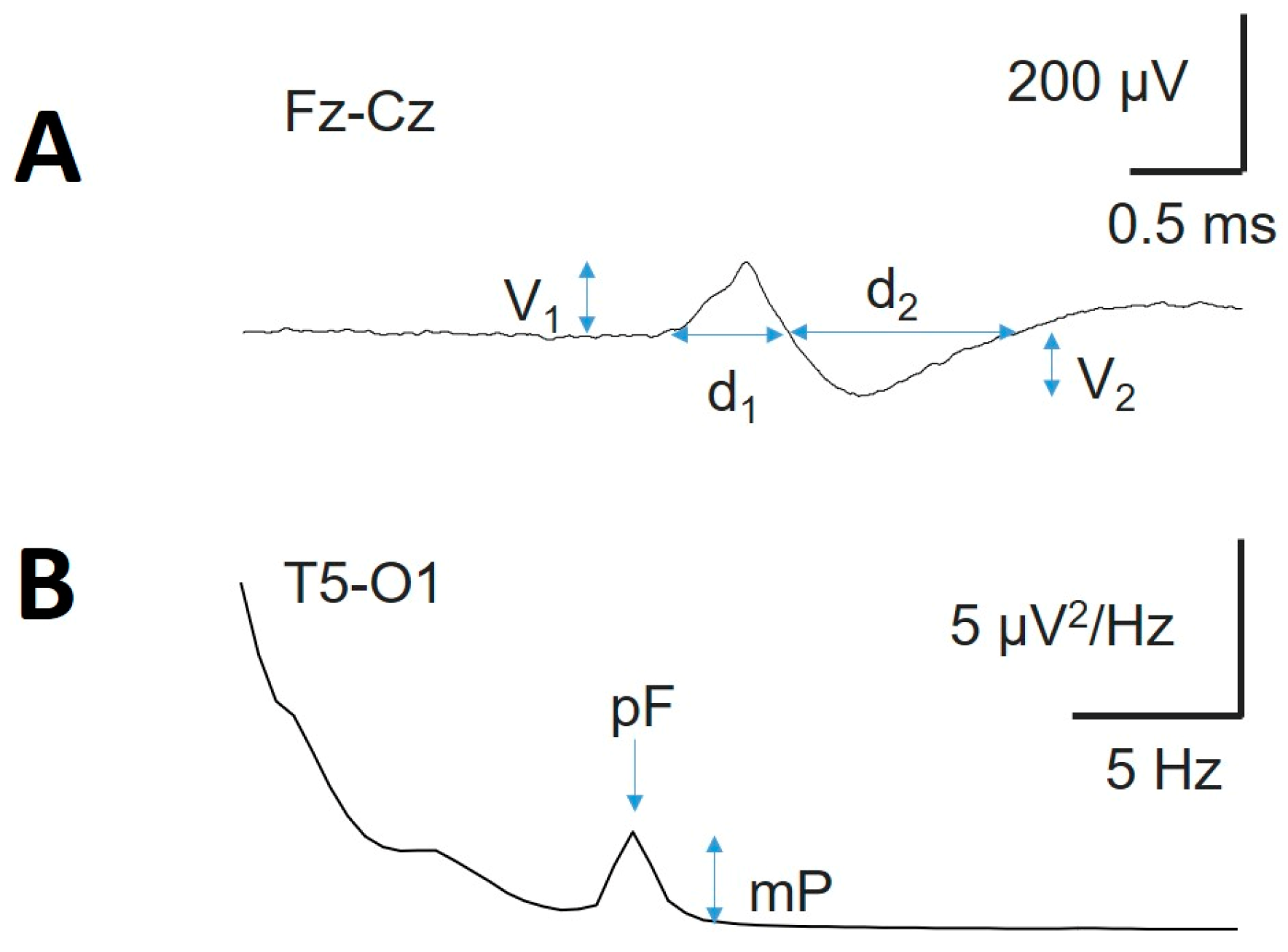
Figure 2.
Comparison between males (red) and females (blue). The left column shows the logPS for all the bands and SSE. Right column: synchronized measurements. A) Wake, B) N1, C) N2, D) N3, and E) REM. L_H = left hemisphere; R_H = right hemisphere, L_F = left frontal; R_F = right frontal, L_PO = left parieto-occipital; R_PO = right parieto-occipital; L_T = left temporal; R_T = right temporal.
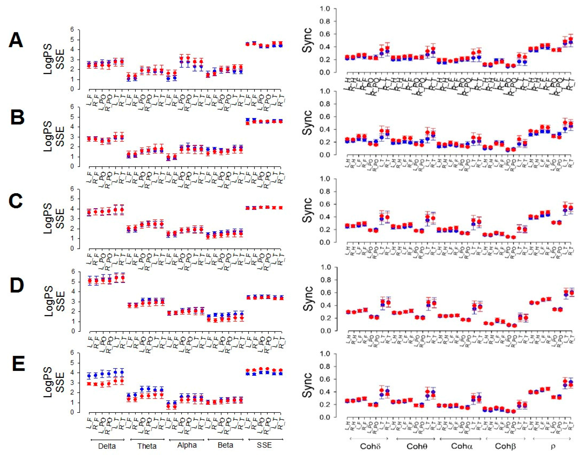
Figure 3.
Box plot for the logPS for the different bands and lobes for the A) wake stage; B) N1; C) N2; D) N3 and E) REM sleep stages. F) δ (upper row) and α (lower row) logPS values during the W stage (dashed box) and REM stage (empty box). *** p < 0.001 for paired Student’s t test. Delta band (δ) = black, theta band (θ) = red, alpha band (α) = blue, and beta band (β) = green. Horizontal lines indicate significant differences between pairs of lobes for the same band; pairs of coloured asterisks (representing the specific bands) indicate significant differences between different bands of the same lobe for Kruskal‒Wallis one-way analysis of variance on ranks and Tukey post hoc tests.
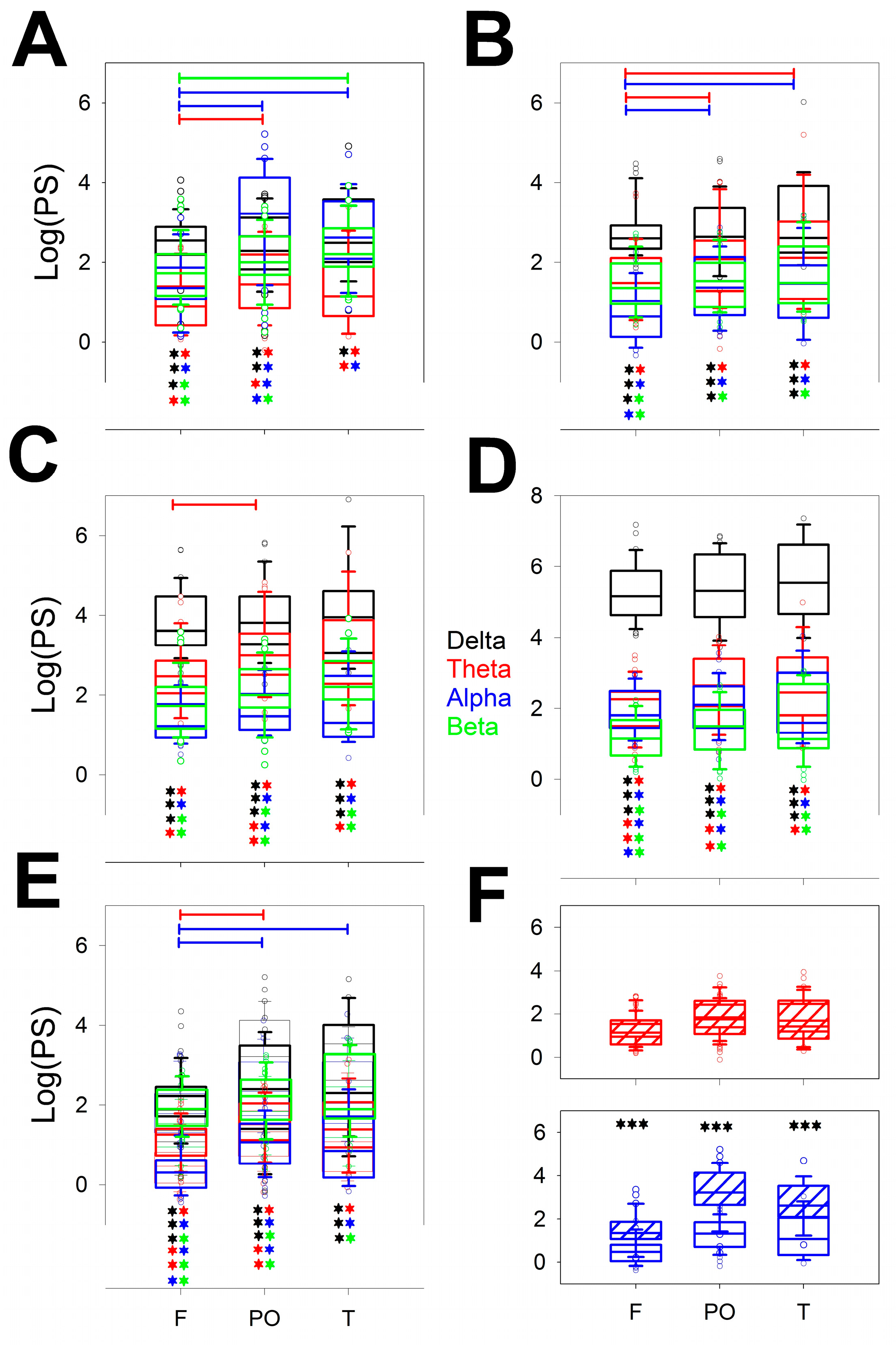
Figure 4.
Box plot for the coherence for the different bands, whole the scalp and lobes for A) different measurements of coherence averaged for the entire scalp; B) coherence during W; C) N1; D) N2; and E) N3 and F) REM sleep stages. Delta band (δ) = black, theta band (θ) = red, alpha band (α) = blue, and beta band (β) = green. Horizontal lines indicate statistical significance between pairs of phases (A) or lobes for the same band; pairs of coloured asterisks (representing the specific bands) indicate significant differences between different bands of the same lobe for Kruskal‒Wallis one-way analysis of variance on ranks and Tukey post hoc tests.
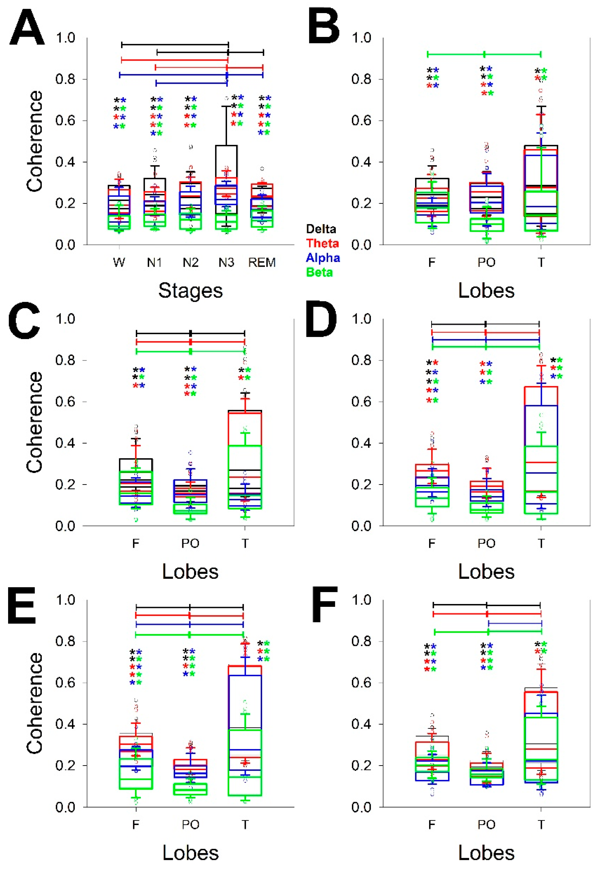
Figure 5.
Box plot for the ρ for the different bands, whole scalp and lobes for A) different measurements of ρ averaged for the entire scalp; B) correlation during W; C) N1; D) N2; E) N3; and F) REM sleep stages. Horizontal lines indicate significant differences between pairs of phases (A) or lobes for the same band for Kruskal‒Wallis one-way analysis of variance on ranks, Tukey post hoc tests.
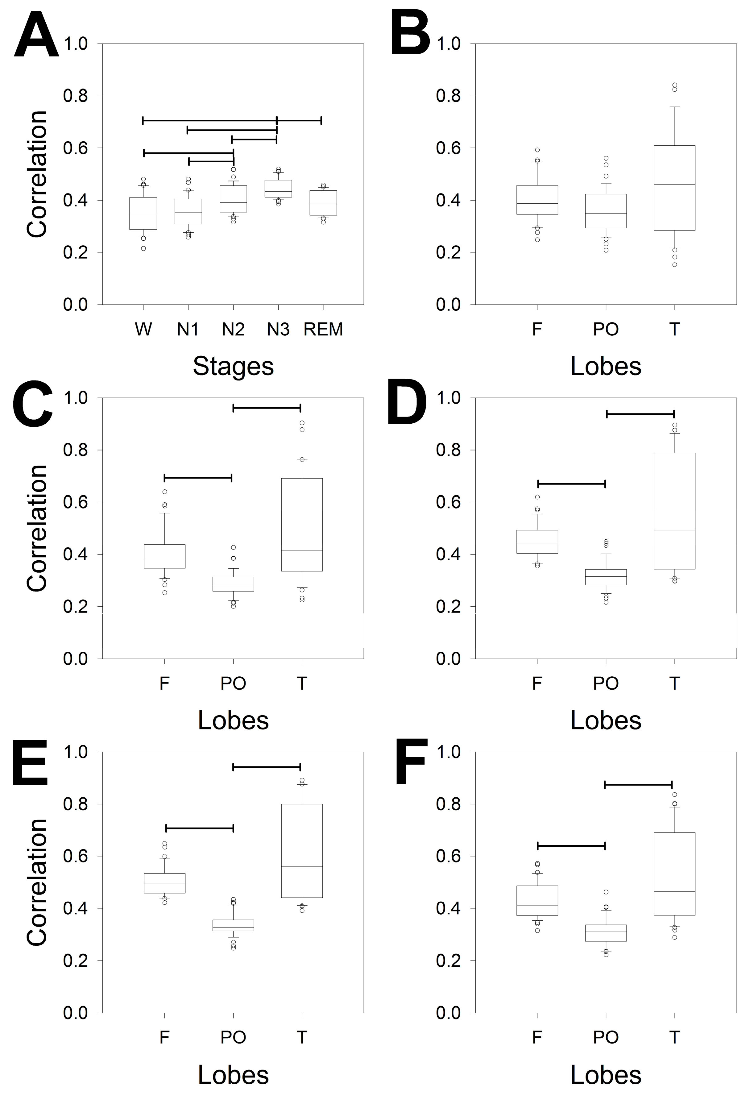
Figure 6.
Box plot for the ρ for the different phases in specific lobes. A) Frontal, B) parieto-occipital and C) temporal lobes. The horizontal lines indicate significant differences between pairs of phases for the Kruskal‒Wallis one-way analysis of variance on ranks and Tukey post hoc tests.
Figure 6.
Box plot for the ρ for the different phases in specific lobes. A) Frontal, B) parieto-occipital and C) temporal lobes. The horizontal lines indicate significant differences between pairs of phases for the Kruskal‒Wallis one-way analysis of variance on ranks and Tukey post hoc tests.
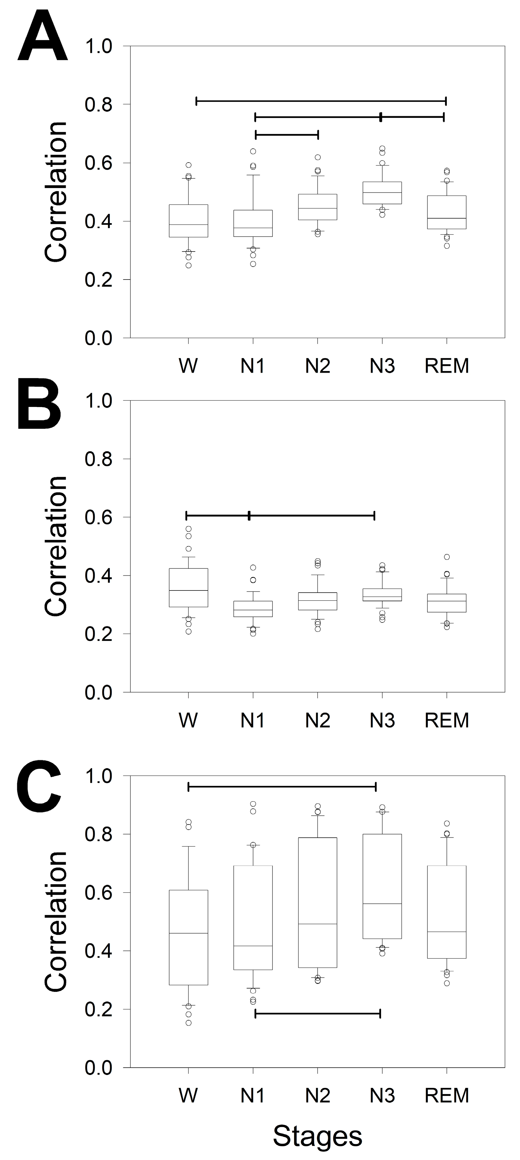
Figure 7.
Mean averaged normalized PS A) Left hemisphere with high vertical gain; B) right hemisphere with high vertical axis gain; C) left hemisphere with lower vertical axis gain; D) right hemisphere with high vertical gain. W = black; N1 = red; N2 = blue; N3 = green; REM = pink. AU = arbitrary units.
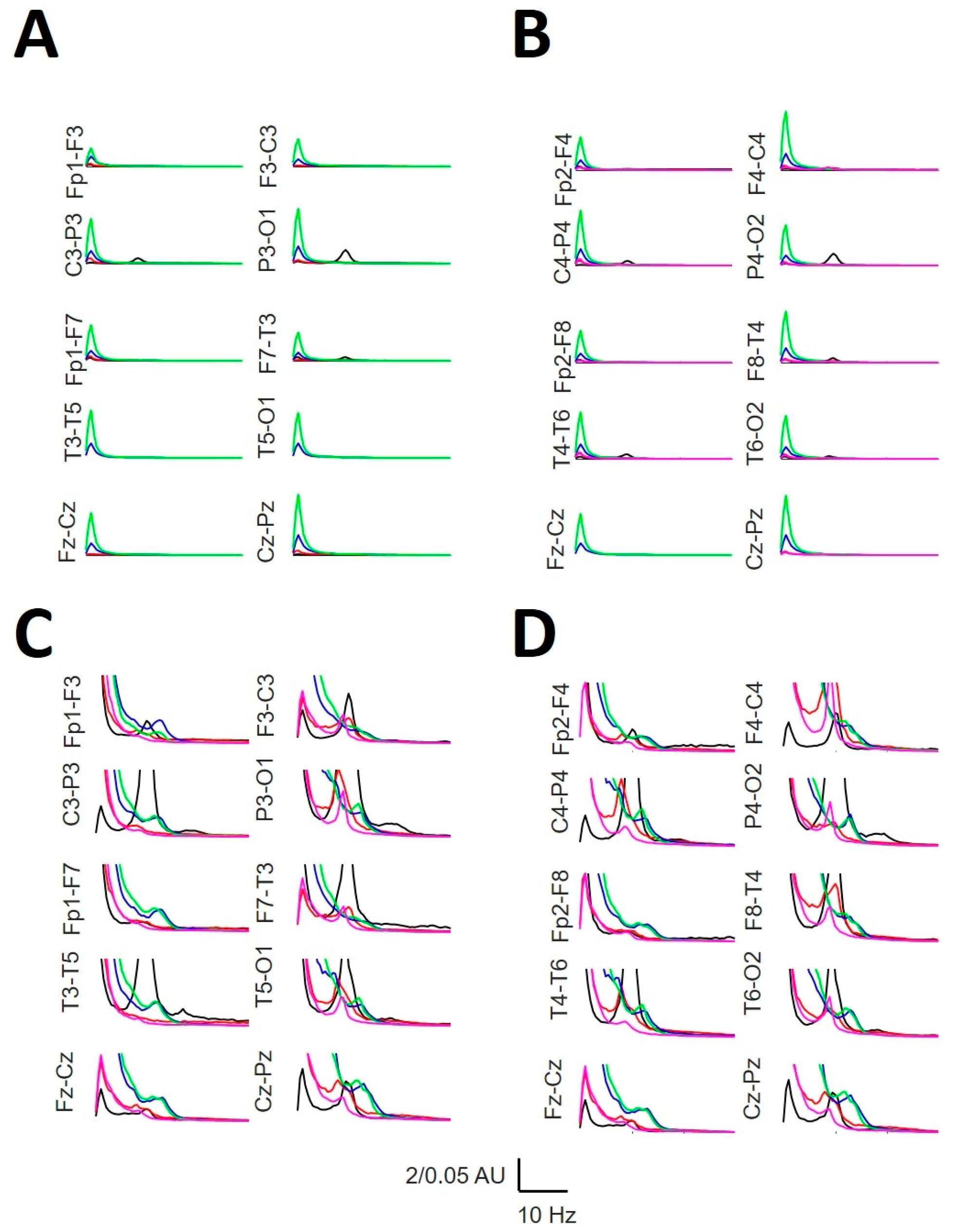
Figure 8.
Maximum differences (maxΔh) for the average PS for every channel. Black = left hemisphere; red = right hemisphere. The inset shows the linear regression between paired channels.
Figure 8.
Maximum differences (maxΔh) for the average PS for every channel. Black = left hemisphere; red = right hemisphere. The inset shows the linear regression between paired channels.
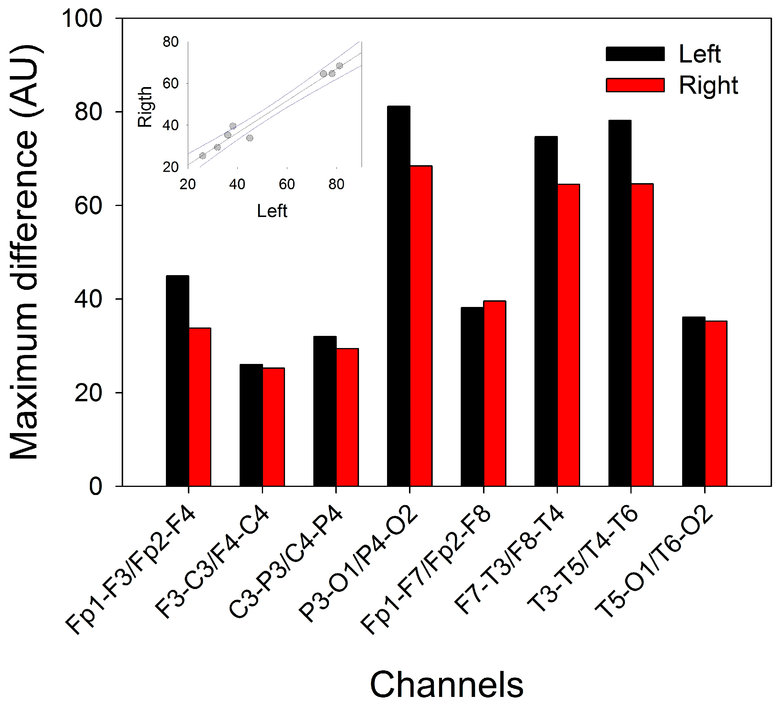
Figure 9.
Numerical properties of KCs. A) Average KCs from a patient; blue lines = left hemisphere, red lines = right hemisphere and green lines = midline. B) Bar graph of the amplitudes of the first (V1, black) and second phases (V2, red). Error bars correspond to the coefficient interval, not the SEM. C) Bar graph for the duration of both phases: d1 (black) and d2 (red). Errors are the CI. D) Linear regression ± 95% confidence band for the amplitude of the first and second components. E) Linear regression ± 95% confidence intervals for the durations of the first and second components. F) Linear regression ± 95% confidence band for the amplitude (V1) and duration (d1) of the first component. G) Linear regression ± 95% confidence band for the amplitude (V2) and duration (d2) of the second component.
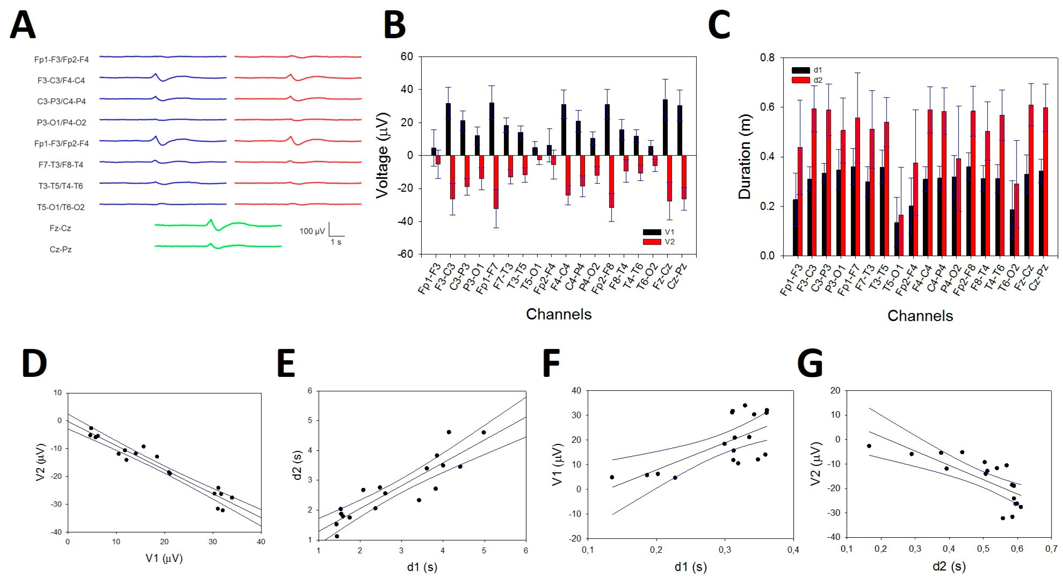
Figure 12.
Relationship between the SS density and the amplitude of the σ band. A) Reconstructed traces from the right hemisphere showing 0% SSs (upper row), 30% SSs (middle row) and 100% SSs (lower row). B) Mean PS from one of the 6 simulations. Red = 0%; green = 25%; blue = 50%; pink = 75%; light blue = 100%. C) Linear regression ± 95% confidence band for the amplitude of PS at the σ band and percentage of SSs at fronto-polar channels (r = 0.9964; p < 3 × 10⁻⁴, function ); D) linear regression ± 95% confidence band for the amplitude of PS at the σ band and percentage of SSs at anterior midline channels (r = 0.9949; p < 4 × 10⁻⁴, function ).
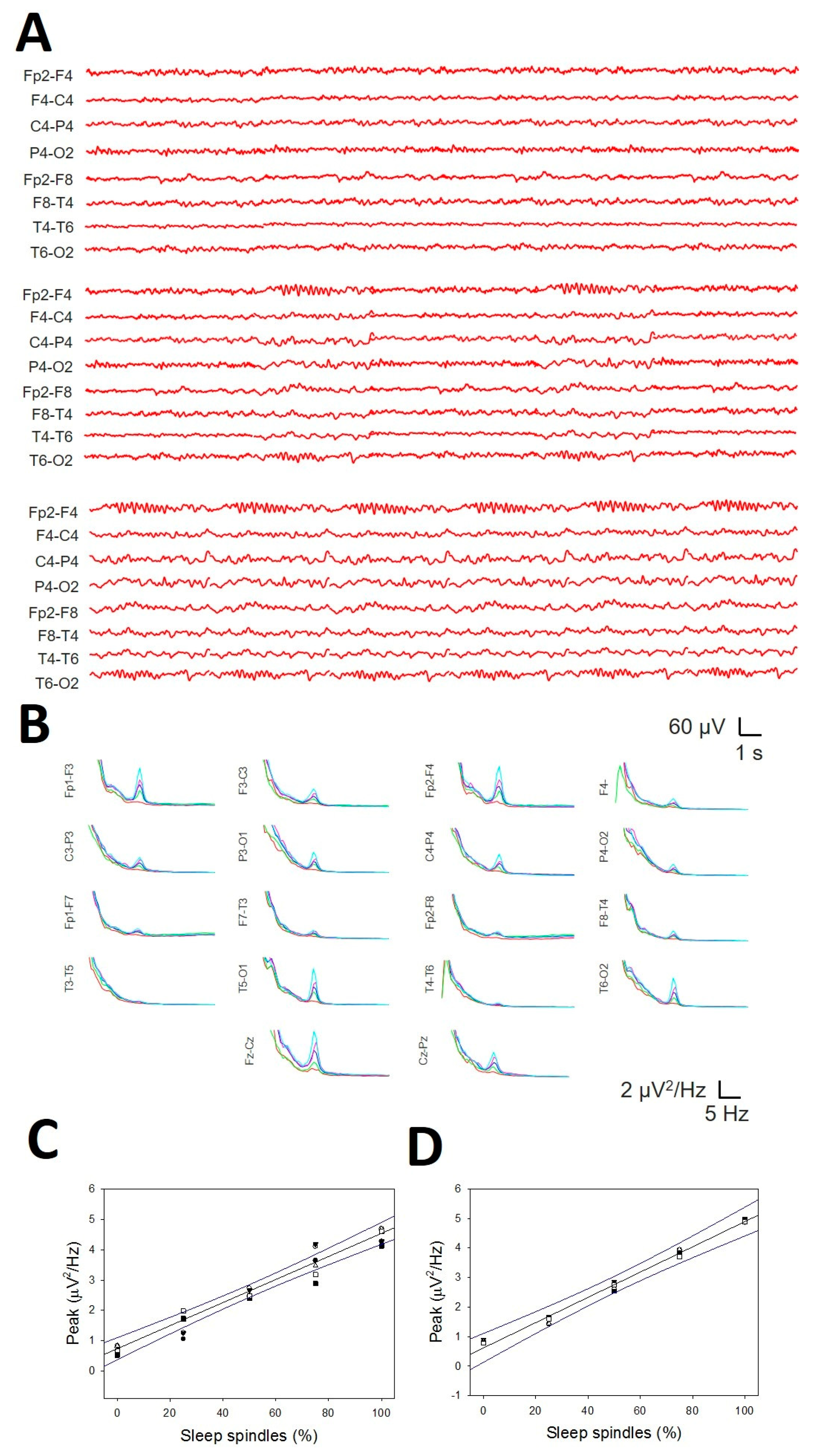
Table 1.
Differences between sexes for whole-scalp logPS, Coh (δ, θ, α and β) and ρ for all stages.
| Stage | logPS | Coh | ρ | ||||||
|---|---|---|---|---|---|---|---|---|---|
| Men | Women | p | Men | Women | p | Men | Women | p | |
| W | 2.18 ± 0.11 | 2.04 ± 0.12 | 0.026 | 0.24 ± 0.07 | 0.22 ± 0.06 | <10-3 | 0.43 ± 0.03 | 0.40 ± 0.02 | n.s |
| N1 | 1.84 ± 0.12 | 1.88 ± 0.12 | n.s | 0.22 ± 0.09 | 0.20 ± 0.06 | <.002 | 0.40 ± 0.04 | 0.37 ± 0.02 | n.s |
| N2 | 2.32 ± 0.19 | 2.34 ± 0.19 | n.s | 0.24 ± 0.10 | 0.22 ± 0.09 | <0.07 * | 0.44 ± 0.05 | 0.42 ± 0.04 | n.s |
| N3 | 2.80 ± 0.31 | 2.99 ± 0.29 | <10-3 | 0.26 ± 0.11 | 0.26 ± 0.11 | n.s | 0.48 ± 0.05 | 0.47 ± 0.04 | n.s |
| REM | 1.68 ± 0.17 | 2.13 ± 0.23 | <10-3 | 0.23 ± 0.09 | 0.23 ± 0.09 | n.s | 0.43 ± 0.04 | 0.43 ± 0.04 | n.s |
n.s. = not significant; * Wilcoxon signed rank test.
Table 2.
Differences between all the paired bands and lobes for logPS. Data are shown as the ratio over the whole number of combinations.
Table 2.
Differences between all the paired bands and lobes for logPS. Data are shown as the ratio over the whole number of combinations.
| Lobe | δ/θ | δ/α | δ/β | θ/α | θ/β | α/β | Σ |
|---|---|---|---|---|---|---|---|
| F | 5/5 | 5/5 | 5/5 | 2/5 | 4/5 | 3/5 | 24/30 |
| PO | 5/5 | 5/5 | 4/5 | 4/5 | 3/5 | 1/5 | 22/30 |
| T | 5/5 | 4/5 | 4/5 | 1/5 | 2/5 | 0/5 | 16/30 |
| Σ | 15/15 | 14/15 | 13/15 | 7/15 | 9/15 | 4/15 | - |
Table 3.
Differences between all pairs of bands and lobes in terms of coherence. Data are shown as the ratio over the number of combinations.
Table 3.
Differences between all pairs of bands and lobes in terms of coherence. Data are shown as the ratio over the number of combinations.
| Lobe | δ/θ | δ/α | δ/β | θ/α | θ/β | α/β | Σ |
|---|---|---|---|---|---|---|---|
| F | 1/5 | 5/5 | 5/5 | 5/5 | 3/5 | 1/5 | 20/30 |
| PO | 0/5 | 4/5 | 4/5 | 3/5 | 5/5 | 3/5 | 19/30 |
| T | 0/5 | 0/5 | 5/5 | 0/5 | 5/5 | 2/5 | 12/30 |
| Σ | 1/15 | 9/15 | 14/15 | 8/15 | 13/15 | 6/15 | - |
Disclaimer/Publisher’s Note: The statements, opinions and data contained in all publications are solely those of the individual author(s) and contributor(s) and not of MDPI and/or the editor(s). MDPI and/or the editor(s) disclaim responsibility for any injury to people or property resulting from any ideas, methods, instructions or products referred to in the content. |
© 2024 by the authors. Licensee MDPI, Basel, Switzerland. This article is an open access article distributed under the terms and conditions of the Creative Commons Attribution (CC BY) license (http://creativecommons.org/licenses/by/4.0/).
Copyright: This open access article is published under a Creative Commons CC BY 4.0 license, which permit the free download, distribution, and reuse, provided that the author and preprint are cited in any reuse.


