
Submitted:
31 December 2025
Posted:
01 January 2026
You are already at the latest version
Abstract
Hot-fluid injection in thermal enhanced oil recovery (TEOR) imposes temperature-driven volumetric strains that can substantially alter in-situ stresses, fracture geometry, and wellbore/reservoir integrity, yet existing TEOR modeling has not fully captured coupled thermo-poroelastic effects on fracture aperture, fracture-tip behavior, and stress rotation within a displacement discontinuity method (DDM) framework. This study develops a fully coupled thermo-poroelastic DDM formulation in which fracture-surface normal and shear displacement discontinuities, together with fluid and heat influx, act as boundary sources to compute time-dependent stresses, pore pressure, and temperature, while internal fracture fluid flow (Poiseuille-based volume balance), heat transport (conduction–advection with rock exchange), and mixed-mode propagation criteria are included. A representative scenario considers an initially isothermal hydraulic fracture grown to 32 m, followed by 12 months of hot-fluid injection with temperature contrasts of ΔT = 0-100 °C and reduced pumping rate. Results show that hydraulic fracture aperture increases under isothermal and modest heating (ΔT = 25 °C) and remains nearly stable near ΔT = 50 °C, but progressively narrows for ΔT = 75-100 °C despite continued injection, indicating potential injectivity decline driven by thermally induced compressive stresses. Hot injection also tightens fracture tips, restricting unintended propagation, and produces pronounced near-fracture stress amplification and re-orientation: minimum principal stress increases by 6 MPa for ΔT = 50 °C and 10 MPa for ΔT = 100 °C, with principal-stress rotation reaching 70–90° in regions above and below the fracture and markedly elevated shear stresses that may promote natural-fracture activation. These findings demonstrate that thermo-poroelastic coupling can govern fracture stability, containment, and injectivity during thermal EOR, motivating temperature-aware geomechanical risk assessment and design for long-term hot-fluid injection operations.
Keywords:
thermal enhanced oil recovery (TEOR)
; hot-fluid injection
; geomechanics
; thermo-poroelasticity
; hydraulic fracturing
; displacement discontinuity method (DDM)
1. Introduction
Rock exhibits volumetric strain when it is exposed to temperature variations. The thermal deformation can be contraction (e.g., in geothermal reservoirs) or expansion (e.g., hot fluid injection for thermal EOR techniques, Figure 1). Such volumetric changes in rock introduce stress changes around the wellbore and in the reservoir and may lead to positive or negative impacts on reservoir flow capacity and wellbore integrity and affect reservoir development plans. In the case of heating the formation, reservoir porosity and permeability may be reduced due to expansion of rock grains into the pore space or be enhanced due to shear fracturing. However, cooling the formation results in improvements to formation porosity and permeability as the rock grains shrink and fractures develop due to shear and tensile stress development [1,2,3]. Heating the rock can cause volumetric changes and dilate the rock. As a result, uplift of the ground by centimeters can be observed in shallow formations [4]. Moreover, thermal loading can result in vertical fractures in the reservoir caprock and affect hydraulic and structural integrity [5]. Laboratory experiments show that the thermal stresses induced by cooling or heating the formation prior to hydraulic fracturing can be used to control the trajectory of fracture propagation [6]. The thermally induced stresses can affect the pressure required to initiate hydraulic fracture, shut-in pressure, and stress estimation using the hydraulic fracturing method [7]. Neglecting thermal loading can lead to overestimation (in the case of cooling the rock) or underestimation (in the case of heating the rock) of rock shear strength [8]. Here, the theory of thermo-poroelasticity is employed to investigate the effects of hot fluid injection on changes in stress magnitude and direction and the evolution of hydraulic fracture aperture over time. Despite extensive work on hydraulic fracturing and thermal recovery, no existing model captures fully coupled thermo-poroelastic effects using the displacement discontinuity method (DDM) on fracture aperture, tip behavior, and stress rotation during long-term hot-fluid injection. This limits our ability to assess geomechanical risks in thermal EOR.
This study offers an original contribution by applying a fully coupled thermo-poroelastic displacement–discontinuity method to thermal enhanced oil recovery for the first time. Although DDM has been used in hydraulic-fracture and geothermal modeling, no previous work has employed this approach to capture the coupled thermal, hydraulic, and poroelastic responses of a hydraulic fracture subjected to hot-fluid injection under thermal-EOR conditions. The formulation used here enables direct quantification of thermally driven aperture evolution, fracture-tip behavior, and stress reorientation during prolonged high-temperature injection, providing a modeling capability that has not previously been available in the thermal-EOR literature.
2. Literature Review
Geomechanical studies can provide important information that may help in EGS management/design and sustaining geothermal reservoir development. Early design of hydraulic fractures developed based on two-dimensional semi-analytical elastic models [9,10]. Over time, and with the advances in computers, complex numerical models have been developed to simulate reservoir stimulation. These numerical simulation approach hydraulic fracture modeling using different methods, including the elastic displacement discontinuity method (DDM) [11,12,13], poroelastic DDM [14,15], thermo-poroelastic DDM [16,17], finite element method [18], extended finite element method [19], discrete element method [20], and hybrid discrete-finite element method [21]. This section presents a review on the elastic, poroelastic, thermoelastic, and thermo-poroelastic numerical techniques used in performing geomechanical study for reservoir stimulation.
Models have been developed based on the theory of elasticity to investigate different aspects in hydraulic fracturing. Sesetty and Ghassemi [22] develops a 2D elastic model to study hydraulic fracture behavior in naturally fractured reservoir. Wu and Olson [23,24] developed an P3D (pseudo-three-dimensional) model to investigate the problem of simultaneous non-planar propagation of multiple hydraulic fractures from HZ wellbore. The 3D correction [25] incorporated into the 2D elastic displacement discontinuity method to account for finite fracture height. They account for fluid flow inside the fracture, and fluid leak-off. Kirchoff’s first and second laws were included in the model to account for the frictional pressure drop in the wellbore and perforations.
The theory of thermo-poroelasticity was employed by Khalaf et al. [26] to simulate hydraulic fracture propagation in geothermal formations and investigate the effects of cold fluid injection on stress changes in magnitude and direction. Abdollahipour et al. [27] developed a poroelastic displacement discontinuity code and calibrated the results against analytical and experimental work. Abdollahipour and Fatehi Marji [28] developed a thermo-poroelastic model verified the model against analytical solutions and field measurements. Tao et al [29,30] used poroelasticity theory to investigate the effect of production from naturally fractured formation on stress-dependent permeability. (Ghassemi and Tao [16] studied the effect change in stresses due to fluid circulation in thermo-poroelastic medium on induced seismicity and permeability variations. Wang and Papamichos [31] presents analytical thermo-poroelastic model to study the transient effects of hot fluid injection on pore pressure and stress development in cylindrical wellbores and spherical cavities of low hydraulic conductivity formation. The results illustrated that hot fluid injection can restrict the development of fractures around wellbores and cavities.
Beyond conventional hydraulic and thermal stimulation, plasma-based stimulation has emerged as an alternative approach for enhancing near-wellbore permeability and creating complex fracture networks. Khalaf et al. [32] conducted integrated experimental and numerical studies on pulsed plasma stimulation, showing that plasma-generated shock waves can initiate and extend fractures, increase fracture conductivity, and modify near-wellbore stress conditions in low-permeability formations. Complementary numerical work by Khalaf et al. [33] analyzed shock-wave stimulation and validated modeled stress and fracture responses against laboratory observations, demonstrating the potential of plasma-based methods as waterless, mechanically efficient stimulation techniques. Although these technologies differ from hot-fluid injection, they share underlying mechanisms involving rapid stress perturbations, fracture opening and closure, and localized stress redistribution, providing additional context for how non-traditional stimulation methods alter fracture geomechanics.
A wide range of studies has examined thermal methods for improving oil recovery in heavy-oil, shale, and other low-mobility reservoirs. These works explore how heat, fluid flow, and rock mechanics interact during processes such as steam injection, hot water flooding, in-situ combustion, thermally assisted fracturing, and hybrid thermal–chemical methods. These studies form the technical foundation for understanding thermal recovery under coupled thermal-hydraulic-mechanical conditions. Geomechanical steam-assisted gravity drainage (SAGD) dilation startup has been applied to create high-permeability flow paths between injector and producer wells. A study in the Karamay oil field examined reservoir geology, geomechanical properties, in-situ stresses, and a six-step high-pressure water-injection process designed to establish dilated zones connecting SAGD well pairs [34]. Laboratory and field evidence highlight that reservoir depth and stress regime primarily control shear-plane orientation and steam-chamber shape [35] [36]. SAGD-related thermal recovery is strongly controlled by thermally induced stress changes, shear dilation, and caprock integrity, and that both field practice and predictive modelling account for geomechanical responses [35,36,37,38,39]. A range of steam and hot-water-based thermal recovery processes has been evaluated in heavy-oil reservoirs. For offshore Bohai heavy oil, hot water chemical flooding has been tested as an alternative to multi–thermal-fluid huff and puff [40]. Steam flooding, cyclic steam stimulation, hot water chemical flooding, and cyclic in-situ combustion can enhance heavy-oil recovery to varying degrees, but their design must balance thermal efficiency, geomechanical effects, and environmental and economic performance [40,41,42,43,44]. In shale environments, thermal and imbibition-based methods interact with complex pore structures and fracture networks, and that rigorous multi-physics modelling is required to properly capture the associated geomechanical and flow responses [45,46]. Stress-dependent fracture behavior, fracture–matrix interaction, and fracture-network geometry are critical controls on thermal EOR injectivity and recovery [39,47,48,49]. Studies highlight that reservoir geomechanics of thermal EOR cannot be considered in isolation from long-term environmental performance and potential post-EOR uses of thermally altered reservoirs [34,43,50].
Across SAGD, steam flooding, cyclic steam stimulation, hot water chemical flooding, and new heating methods, the studies consistently show that thermal loading modifies stresses, induces shear and dilation, alters fracture permeability, and changes rock and fluid properties in ways that strongly affect injectivity, steam- or heat-chamber development, and ultimate recovery [35,36,37,38,39,45,49,50]. Coupled numerical models of varying complexity demonstrate that explicitly accounting for stress–flow–temperature interactions and fracture-network geomechanics is essential for reliable prediction of thermal EOR performance and for assessing caprock integrity and surface deformation [35,36,39,47,49]. At the same time, environmental and energy-transition considerations impose additional constraints and objectives on the design of thermal EOR projects [34,43,50]. Within this context, there remains a need for detailed thermo–poroelastic analyses that explicitly quantify stress evolution and hydraulic fracture aperture changes during long-term hot-fluid injection, especially in settings where both reservoir performance and containment depend on the coupled geomechanical response. The studies summarized here provide the necessary background on thermal processes, fracture behavior, and coupled modelling approaches that inform such analyses.
This study advances current knowledge by applying a fully coupled thermo-poroelastic displacement discontinuity method to thermal enhanced oil recovery conditions for the first time. While DDM has been widely used in hydraulic fracturing and geothermal applications, it has not previously been applied to thermal-EOR operations. The framework adopted here enables direct simulation of thermally driven fracture-aperture evolution, fracture-tip tightening, and rotation of the local in-situ stress field over extended injection periods. Consequently, the work provides a new modeling capability that clarifies how thermal stresses can govern fracture stability, injectivity, and the potential activation of surrounding natural fractures under realistic thermal-EOR temperature contrasts.
3. Methodology
The model describes a hydraulic fracture embedded in a thermo-poroelastic rock. The rock matrix is governed by the coupled thermo-poroelastic field equations (momentum, mass, and heat) and their constitutive relations [1,51]. The solution is obtained using an indirect boundary element formulation, the Displacement Discontinuity Method (DDM), which acts only on the fracture boundary [1,51,52]. The fracture itself carries normal and shear displacement discontinuities and exchanges fluid and heat with the surrounding rock. Inside the fracture, fluid flow [15] and heat-transport [53] equations are used, and fracture propagation is included through a mixed-mode propagation criterion [54,55]. A detailed description of the thermo-poroelastic methodology can be found in [17].
3.1. Boundary-Element Formulation with DDM
The fracture boundary is discretized into N straight elements. Each element has local normal and tangential directions and carries normal displacement discontinuity , shear displacement discontinuity , fluid influx , and heat influx . These quantities act as sources in the thermo-poroelastic matrix. Stresses, pore pressure, and temperature at any point on or near the fracture are obtained from thermo-poroelastic fundamental solutions integrated over space and time along the boundary (Figure 2).
The general thermo-poroelastic boundary-integral equations for stress, pore pressure, and temperature can be written as follows [56]:
where, represents the normal or shear stress at location x and time t, obtained by summing the effects of instantaneous displacement discontinuities , fluid-induced stresses , and heat-induced stresses . The fracture boundary is denoted by Γ, and the coordinates x and χ identify points in the two-dimensional plane. The influence functions , , and correspond respectively to displacement discontinuity, fluid influx, and heat influx. The superscripts id, if, and ih specify whether each contribution originates from mechanical, fluid, or thermal processes. These boundary integral equations are solved numerically using spatial and temporal discretization. In these equations, the stress (normal or shear), pore pressure, and temperature at a point i and time t are expressed as integrals of the displacement discontinuities, fluid sources, and heat sources on the fracture. The influence functions appearing in Equation (1)-(3) represent the response in stress, pressure, or temperature at i caused by unit displacement discontinuity, fluid influx, or heat influx at each boundary element j. Separate influence functions are used for mechanical, hydraulic, and thermal contributions [17].
3.2. Numerical Implementation of DDM
For numerical implementation, the fracture boundary is divided into N elements of half-length , and the time domain is split into discrete time levels (, , ,…etc.) (Figure 2). Within each time step, normal and shear displacement discontinuities and fluid and heat influxes are assumed constant on each element. The time-dependent boundary-integral equations are written in incremental form: at each time step, only the increments of displacement discontinuities and fluxes are unknowns, while the influence of all previous increments is accounted for as history. Let element i be influenced by element j. The incremental normal and shear stresses, pore pressure, and temperature at element i at time step k are given by Equations (4)-(7). The resulting stresses, pore pressure, and temperature at from sources at are expressed as follows:
In this expression, , , and represent the incremental normal and shear displacement discontinuities, along with the incremental fluid and heat influxes, applied during time step h. The terms , , , , , , , , , , and denote the corresponding influence coefficients that quantify how the j-th element affects the i-th element at the same time step h [57,58]. In these expressions, the incremental normal and shear displacement discontinuities and the incremental fluid and heat influxes at element j and time step are multiplied by influence coefficients. Each influence coefficient represents the contribution of unit displacement discontinuity, unit fluid influx, or unit heat influx on element j, applied at a given time, to the normal or shear stress, pore pressure, or temperature at element i at the current time step. The entire history of loading is included by summing contributions over all previous time steps. A detailed description of the influence coefficients mathematical formulation and physical meaning is provided by Khalaf [17].
At a given time, total normal and shear displacement discontinuities and fluxes on each element are obtained by summing their increments over all past time steps, as expressed compactly as follows:
Equation (8) defines the cumulative values of normal displacement discontinuity (hence fracture width), fluid influx, and heat influx as simple sums of their incremental values. This incremental–cumulative structure allows the time-dependent thermo-poroelastic response to be captured efficiently in a time-marching scheme. At each new time step, contributions from all previous increments are subtracted from the prescribed boundary conditions, leaving a linear system for the new increments, which is then solved for displacement discontinuities and fluxes.
3.3. Fracture Propagation Criteria
Fracture propagation is modeled using a mixed-mode fracture criterion based on stress intensity factors for Modes I and II [59]. Under fluid injection, fracture pressure and width increase, raising the Mode I and Mode II stress intensity factors and at the fracture tips (Figure 3). Propagation occurs when a combined measure of these stress intensity factors exceeds the fracture toughness [54,55]. The governing propagation condition is written as follows:
The direction of fracture propagation is defined by an angle θ measured from the original fracture orientation. The propagation angle is computed from a closed-form expression involving and based on the maximum principal stress criterion. This expression is given as follows:
where , and . Using Equations (9) and (21), the model checks at each time step whether the stress intensity at a tip exceeds the critical value. If so, the fracture is extended by a finite length in the direction given by the angle θ, and new DDM elements are added to the boundary to represent the longer fracture.
3.4. Fluid Flow Inside the Fracture
Fluid flow within the hydraulic fracture is modeled using Poiseuille’s law together with a segment-wise volume balance. Each fracture element is treated as a one-dimensional conduit in which flow is driven by pressure gradients along the element, and coupled to the surrounding rock by leak-off. The volume-balance equation combines the effects of fluid compressibility, fracture width change, leak-off, and direct injection or production [15]. It can be written as:
In this equation, fracture permeability () and width () characterize the hydraulic properties of the fracture. The element half-length () a specifies the spatial resolution along the fracture. Fluid compressibility () and fracture pressure () control the storage and pressure response within the fracture, while additional terms represent fluid leak-off () into the surrounding medium and any prescribed fluid sources (). In Equation (11), the left-hand side represents the net flow along the fracture element, computed from the local fracture permeability (or hydraulic conductivity) and width using Poiseuille’s law. The right-hand side consists of four terms: (1) the change in fluid volume due to fluid compressibility, (2) the change in fracture volume caused by evolution of fracture width (normal displacement discontinuity), (3) leak-off from the fracture into the surrounding porous matrix, and (4) external sources or sinks representing injection or production. This equation is applied independently to each fracture element at each time step, using fracture width and leak-off from the DDM solution and solving for fracture pressure and flow rate.
3.5. Heat Transfer Inside the Fracture
Heat transport within the fracture is governed by an energy balance that includes conduction, advection by the moving fluid, and heat exchange with the rock [53]. The fracture-scale heat balance equation is given as:
The formulation uses the fracture element half-length a, together with the fracture width () and the volumetric flow rate inside the fracture (), to describe fluid transport. Fluid density (), compressibility (), and thermal conductivity () determine how mass and internal energy are transported within the fracture system. Heat loss or gain to the formation is represented by , while is the local fluid temperature. This formulation ensures accurate tracking of thermal transport under dynamic flow and rock-fluid interactions. In Equation (12), the left term represents transient storage of thermal energy in the fluid. The first term on the right represents thermal conduction along the fracture, the second term represents advective transport of heat along the fracture due to fluid flow, and the last term represents heat exchange between the fracture fluid and the surrounding rock
4. Results and Analysis
This section presents an example used to investigate the effects of injecting hot fluid into a colder formation on stress changes and their impact on fracture aperture. One of the main applications of hot fluid injection into underground formations is enhanced oil recovery. The example considered here involves a hydraulic fracture that is propagated using fracturing fluid at the same temperature as the reservoir (an isothermal hydraulic fracturing process). The formation’s physical, mechanical, and thermal properties are listed in Table 1. The hydraulic fracture is allowed to grow to a length of 32 meters (Figure 4). After reaching 32 meters, hot fluid is injected for 12 months at temperatures ranging from 25 to 100 °C above the reservoir temperature. The pumping rate during the isothermal fracture propagation stage is 8 bbl/d/m-thickness. This rate is then reduced to 4 bbl/d/m-thickness during the hot fluid injection stage.
The evolution of the maximum fracture width during the fracture propagation and fluid injection stages is shown in Figure 5 on a semi-log graph. In this figure, in addition to the isothermal injection case (ΔT=0), the fracture width is plotted for four different temperature differences between the hot injection fluid and the colder formation, ranging from 25 to 100 °C. The isothermal injection case is represented by the red line. The blue and green lines correspond to the 25 and 50 °C cases, respectively, while the 75 and 100 °C cases are shown by the black and brown lines, respectively.
The width evolution curve is divided into two parts. The first part represents the fracture propagation stage with a pumping rate of 8 BPD/m-thickness. The second part represents the fracture width during the subsequent fluid injection stage with a pumping rate of 4 BPD/m-thickness. At the end of the fracture propagation stage, the maximum fracture aperture is approximately 0.71 mm. When the flow rate is reduced (from 8 BPD/m-thickness during propagation to 4 BPD/m-thickness during fluid injection), the fracture aperture exhibits a drop over a short period of time.
Examining the change in fracture aperture during the fluid injection stage shows that the aperture increases continuously in the 0 and 25 °C injection cases. For the 50 °C case, the aperture shows a small increase and then remains almost constant. In contrast, for the 75 and 100 °C cases, the aperture decreases over time, even though fluid continues to be injected into the formation through the fracture. This reduction in fracture aperture over time during hot fluid injection can decrease well injectivity. The reduction is caused by the significant increase in stress that develops around the fracture due to thermal expansion of the formation material (as discussed later in this paper).
At the end of the 12-month injection period, the distribution of fracture width along the fracture length is shown in Figure 6. The curves are almost equally spaced over most of the fracture length. In addition, the fracture tips are narrower at the end of the hotter fluid injection cases, which restricts unintentional fracture propagation during hot fluid injection. In contrast, the increase in fracture tip width in the isothermal injection case can promote further fracture propagation during fluid injection.
At the end of the 12-month injection period, Figure 7 presents contour maps of the magnitude of the minimum principal stress and the direction of the maximum principal stress in a 120 m×120 m area around the hydraulic fracture. In these contour maps, the direction of the maximum principal stress is shown as dashes, while the hydraulic fracture is represented as a white line. The minimum principal stress is critical because, in the injection-affected region, propagation of new fractures requires the pumping pressure to exceed the updated minimum principal stress. In a two-dimensional problem, these new fractures follow the direction of the maximum principal stress. Initially, the minimum principal stress is 25 MPa and the direction of the maximum principal stress is along the x-direction (parallel to the hydraulic fracture).
Compared with the isothermal injection case shown in Figure 7, the hot fluid injection process causes a significant re-orientation of the maximum principal stress direction and considerable changes in the minimum principal stress (a negative stress value in the contour maps denotes compression). Hot fluid injection with ΔT=50°C (Figure 7-B) for 12 months raises the minimum principal stress by approximately 6 MPa in the region around the fracture, while for ΔT=100°C (Figure 7-C) the increase reaches approximately 10 MPa. In contrast, the increase in stress for the isothermal injection case (Figure 7-A) is less than 2.5 MPa close to the fracture. In addition to hydraulic loading, the increase in stress during high-temperature fluid injection is attributed to thermal expansion of the reservoir material.
The results also show that the upper and lower parts of the contour maps (on the two sides of the fracture) experience the most significant increases in minimum principal stress, whereas the areas to the left and right (along the fracture extent) exhibit only small changes in minimum principal stress. Furthermore, examination of the rotation of the maximum principal stress indicates that the direction of the maximum principal stress is re-oriented by an angle almost everywhere on the map, except in the regions directly above and below the fracture and along its extent in the x-direction. This rotation in the orientation of the maximum principal stress can be explained by analyzing the changes in the normal stresses (, ) and the shear stress () induced by the fluid injection process.
The changes in the normal stress in the x-direction (Δ) induced in the formation around the hydraulic fracture are shown in Figure 8. The figure illustrates that the normal stress undergoes a large increase in the region close to the fracture. This increase in stress becomes larger as the temperature difference increases. The peak increases are 2.8, 10, and 18 Mpa for the cases of ΔT=0, 50, and 100 °C, respectively. The isothermal injection case shows an increase in stress throughout the entire plotted area, with a minimum increase of 1.2 Mpa. However, in the 100 °C case, the very green spots on the contour map exhibit a small reduction (positive change in stress) from the initial state. It is important to note that the stress in the x-direction is no longer the maximum principal stress, because the fluid injection causes a re-orientation of the principal stresses (Figure 7-C).
On the other hand, Figure 9 shows that the normal stress change in the y-direction (Δ) exhibits a different behavior. The increase in is smaller than the increase in . As seen from the contour maps in Figure 8 and Figure 9, for ΔT=0°C, the peak increases around the fracture are 2.8 and 2.4 Mpa for and , respectively. For ΔT=100°C, the increases in and around the fracture are 18 and 10 Mpa, respectively. In addition, in contrast to the distribution of Δ, the largest increases in occur in the upper and lower parts of the map. Only minor changes in are observed in regions near the x-axis during hotter fluid injection, which is attributed to the rotation of the principal stress direction.
Another parameter that contributes to the re-orientation of the maximum principal stress is the shear stress that develops during the fluid injection process, as shown in Figure 10. In this figure, the shear stress induced by fluid injection that is 100 °C hotter than the reservoir (Figure 10-C) is almost double the magnitude of the shear stress in the 50 °C case (Figure 10-B) and 10 times the magnitude of the isothermal injection case (Figure 10-A). The figure also indicates that the change in shear stress is largest around the fracture tips and relatively minor along the two axes (x-axis and y-axis). This change in shear stress plays a major role in the activation of natural fractures present in underground formations, which can increase the injectivity of injection wells and emphasizes the strong influence of temperature contrast on shear stress development.
For further clarification of the stress changes, the stresses and the principal stress rotation angle are evaluated along two lines on the contour maps. The first line is taken parallel to the y-axis (at x=1), starting at point (1,1) and ending at point (1, 300), and the results are presented in Figure 11 and Figure 12. The second line is parallel to the x-axis, at y=1, starting at (1,1) and ending at (300,1), and the results are presented in Figure 13 and Figure 14.
In Figure 11, for the three fluid injection cases (ΔT=0,50 and 100°C), the changes in the normal stress in the x-direction (), the normal stress in the y-direction (Δ), and the shear stress () are plotted as blue, red, and green lines, respectively. Under the initial conditions, the normal stress in the x-direction (, the initial maximum principal stress) is higher than the normal stress in the y-direction (, the initial minimum principal stress) by 3 MPa, reflecting the initial stress anisotropy. The 12-month injection period modifies both the magnitudes and directions of the stresses. For the isothermal injection process (ΔT=0) along the line x=1, Figure 11-A shows increases in both normal stresses and (the negative sign in the figure indicates compression). Closer to the fracture, the increase in is greater than the increase in . As the distance from the fracture increases along x=1, the opposite behavior is observed, with the increase in exceeding the increase in . However, the difference between the normal stress curves stabilizes to less than 1 MPa. This small difference keeps higher than by ≈2 MPa, so the re-orientation of the principal stress direction mainly depends on the shear stress.
The development of shear stress is shown by the green line in the figure and remains small in magnitude (with a peak value of ≈0.022 MPa). As a consequence, only a small reorientation (≅0.45° at its maximum) of the direction of the maximum principal stress is observed, as indicated by the green line in Figure 12-A. The rotation angle of the principal stress varies in direct relation to the shear stress magnitude, and the maximum rotation angle of the maximum principal stress occurs where the shear stress reaches its peak value.
In the hot injection cases (ΔT=50 and 100 °C), a significant rotation of the maximum principal stress direction is observed. This behavior is attributed to the large changes in and and the relatively large development of shear stress. For ΔT=50°C, the rotation of the maximum principal stress from its initial direction reaches 70° (Figure 12-B) at a distance of 30 m from the fracture along x=1. At this location, Figure 11-B shows that the increase in exceeds the increase in by almost 3 MPa, which is sufficient to overcome the initial stress anisotropy. In addition, the shear stress developed due to hot fluid injection is several times larger than in the isothermal injection case, further promoting stress re-orientation.
Similarly, the 100 °C injection case causes an approximately 90° rotation of the maximum principal stress direction over a longer distance along x=1 (Figure 12-C). At larger distances from the hydraulic fracture, the difference between the normal stresses stabilizes to less than 3 MPa (the initial stress anisotropy), and the change in shear stress diminishes. As a result, the rotation of the maximum principal stress direction becomes minimal in the far field.
In Figure 12, the maximum and minimum principal stresses are shown by the blue and red curves, respectively. Significant increases in both minimum and maximum principal stresses are observed in the region close to the fracture. The maximum principal stress 1 m away from the fracture along x=1 is 31, 39, and 47 Mpa for ΔT=0, 50, and 100°C, respectively. The corresponding peak values of the minimum principal stress are 27.5, 32, and 35 Mpa for ΔT=0, 50, and 100°C, respectively. The magnitudes of both principal stresses decrease with increasing distance from the fracture and eventually return to their initial values, indicating the spatially localized nature of the thermally induced stress perturbations around the fracture.
In contrast to the behavior along x=1, Figure 13 shows that along the line y=1 the increase in is greater than the increase in . On one hand, the difference between the increases in and becomes larger for hotter injection cases, which resists the re-orientation of the principal stress (i.e., it reduces the rotation angle). On the other hand, hotter fluid injection generates larger shear stress, which tends to promote stress re-orientation.
Despite the higher shear stresses under hotter injection, Figure 14 indicates that the rotation angle of the maximum principal stress remains small. This is because the increase in the difference between the two normal stresses is large and exceeds the magnitude of the shear stress, thereby limiting the amount of principal stress rotation. The minimum and maximum principal stresses along the line y=1 exhibit large changes in magnitude near the fracture, but these changes diminish progressively as the distance from the fracture increases.
Figure 15 presents the temperature contour maps at the end of the 12-month hot injection period. The figure indicates that the increase in temperature is mainly concentrated around the hydraulic fracture, forming a pronounced thermal anomaly in its vicinity. The heat spreads in an elliptical pattern around the fracture, reflecting the combined effects of conduction and the geometry of the fracture. It can also be observed that the corners of the contour map experience only very minor changes in temperature, highlighting the localized nature of the thermal influence of hot fluid injection around the fracture.
5. Discussion
This advancement clarifies how strongly coupled thermo-poroelastic processes during hot-fluid injection can reshape stress fields and fracture geometry in thermal EOR operations. The simulations show that thermal expansion of the rock around a hydraulically created fracture can increase compressive stresses by more than an order of magnitude compared with isothermal injection, rotate the principal stresses by 70–90° above and below the fracture, and significantly tighten fracture apertures and tips over a 12-month injection period.
The fracture aperture results indicate that hot-fluid injection does not simply preserve or enlarge fracture conductivity relative to an isothermal case. For modest temperature contrasts (ΔT = 25–50 °C), fracture width can still increase or remain nearly constant, but for higher temperature contrasts (ΔT = 75–100 °C) the thermally induced increase in compressive stress dominates, leading to progressive narrowing of the fracture despite ongoing injection. The narrowing is most pronounced at the fracture tips, where thermal stresses tighten the fracture and suppress further propagation. This behavior implies that operators may see declining injectivity over time under hot injection, and that thermally tightening tips can improve vertical and lateral containment by reducing the likelihood of unintended fracture growth during prolonged thermal EOR stages.
The stress-field analysis shows that hot-fluid injection produces much larger normal and shear stress changes than isothermal injection and that these changes are strongly anisotropic around the fracture plane. Minimum principal stress increases are concentrated above and below the fracture, while regions along the fracture length experience smaller changes, reflecting the elliptical thermal halo around the fracture. The associated shear stresses (up to an order of magnitude higher than in the isothermal case) drive substantial rotation of the principal-stress directions in the near-fracture region. This stress rotation favors activation and shear dilation of nearby natural fractures in specific sectors around the hydraulic fracture, which can enhance lateral injectivity and create additional flow pathways, but may also redirect flow away from the intended target zone if well placement and injection strategy do not account for these patterns.
6. Conclusions
The theory of thermo-poroelasticity is used to investigate the effects of hot fluid injection on stress development within a porous medium. The model fully couples three processes: the mechanical process (relating the stresses applied to the fracture surface to the corresponding deformation), the fluid-flow process (accounting for fluid movement from the fracture into the formation and through the permeable formation), and the thermal process (calculating heat transfer from the fracture into the formation and within the formation). Poiseuille’s equation is incorporated to evaluate fluid flow inside the fracture, and fracture propagation based on the maximum stress criterion is also included. A representative example of hot fluid injection into an underground formation highlights the model’s ability to capture the complex interactions among thermal, hydraulic, and mechanical effects, providing a comprehensive basis for assessing thermal EOR geomechanics in subsurface systems.
First, the results show that fracture width, and therefore well injectivity, can decrease over time due to excess stresses generated by thermal expansion of the surrounding formation. This finding underscores the practical significance of the model: it demonstrates that injectivity decline is not merely a function of operational parameters but can be strongly controlled by thermo-mechanical coupling, a factor often overlooked in conventional engineering design.
Second, the narrowing of fracture tips during hot injection limits further fracture propagation, improving the containment of the stimulated region. However, prolonged injection of colder fluid can reverse this effect, widening the tips and enabling unintended propagation. This dual behavior highlights the value of the work by illustrating how even modest temperature variations can shift fracture stability, offering crucial guidance for temperature management in long-term thermal operations.
Third, hot fluid injection causes substantial changes in the initial stress field, leading to the development of large shear stresses and a significant re-orientation of the maximum principal stress direction compared to isothermal injection. This stress rotation enhances the likelihood of activating natural fractures through shear deformation. By revealing these thermally induced stress-path deviations, the study provides meaningful insights for designing safer, more predictable thermal enhanced recovery processes and for improving geomechanical risk assessments in heat-injection projects.
Data Availability Statement
The original contributions presented in this study are included in the article. Further inquiries can be directed to the corresponding author.
Conflicts of Interest
The author declares no conflicts of interest.
References
- Palciauskas, V. V.; Domenico, P.A. Characterization of Drained and Undrained Response of Thermally Loaded Repository Rocks. Water Resour. Res. 1982, 18, 281–290. [CrossRef]
- Azad, A.; Chalaturnyk, R.J. Numerical Study of SAGD: Geomechanical-Flow Coupling for Athabasca Oil Sands Reservoirs. In Proceedings of the 45th US Rock Mechanics / Geomechanics Symposium; 2011.
- Lee, S.H.; Ghassemi, A. Thermo-Poroelastic Finite Element Analysis of Rock Deformation and Damage. In Proceedings of the 43rd U.S. Rock Mechanics Symposium and 4th U.S.-Canada Rock Mechanics Symposium; ARMA 09-121 paper was prepared for presentation at Asheville 2009, the 43rd US Rock Mechanics Symposium and 4th U.S.-Canada Rock Mechanics Symposium, held in Asheville, NC June 28th – July 1, 2009, 2009.
- Butler, R.M. Expansion of Tar Sands During Thermal Recovery. J. Can. Pet. Technol. 1986, 25, 51–56. [CrossRef]
- Li, B.; Wong, R. Effect of Thermally Induced Deformation of Shale on Wellbore and Caprock Integrity. In Proceedings of the All Days; SPE, June 11 2013; Vol. 1, pp. 149–158.
- Wu, R.; Germanovich, L.N.; Van Dyke, P.E.; Lowell, R.P. Tharmal Technique for Controlling Hydraulic Fractures. J. Geophys. Res. Solid Earth 2007, 112, 1–15. [CrossRef]
- Stephens, G.; Voight, B. Hydraulic Fracturing Theory for Conditions of Thermal Stress. Int. J. Rock Mech. Min. Sci. Geomech. Abstr. 1982, 19, 279–284. [CrossRef]
- Tao, Q.; Ghassemi, A. Poro-Thermoelastic Borehole Stress Analysis for Determination of the in Situ Stress and Rock Strength. Geothermics 2010, 39, 250–259. [CrossRef]
- Geertsma, J.; De Klerk, F. A Rapid Method of Predicting Width and Extent of Hydraulically Induced Fractures. J. Pet. Technol. 1969, 21, 1571–1581. [CrossRef]
- Perkins, T.K.; Kern, L.R. Widths of Hydraulic Fractures. J. Pet. Technol. 1961, 13, 937–949. [CrossRef]
- Keh-Jian Shou; Siebrits, E.; Crouch, S.L. A Higher Order Displacement Discontinuity Method for Three-Dimensional Elastostatic Problems. Int. J. rock Mech. Min. Sci. Geomech. Abstr. 1997, 34, 317–322. [CrossRef]
- Wu, K.; Olson, J.E. Mechanics Analysis of Interaction between Hydraulic and Natural Fractures in Shale Reservoirs. Soc. Pet. Eng. - SPE/AAPG/SEG Unconv. Resour. Technol. Conf. 2016. [CrossRef]
- Olson, J.E.; Wu, K. Sequential versus Simultaneous Multi-Zone Fracturing in Horizontal Wells: Insights from a Non-Planar, Multi-Frac Numerical Model. In Proceedings of the Society of Petroleum Engineers - SPE Hydraulic Fracturing Technology Conference 2012; SPE, February 6 2012; pp. 737–751.
- Kanaun, S. On the Hydraulic Fracture of Poroelastic Media. Int. J. Eng. Sci. 2020, 155. [CrossRef]
- Kamali, A.; Ghassemi, A. On the Role of Poroelasticity in the Propagation Mode of Natural Fractures in Reservoir Rocks. Rock Mech. Rock Eng. 2020, 53, 2419–2438. [CrossRef]
- Ghassemi, A.; Tao, Q. Thermo-Poroelastic Effects on Reservoir Seismicity and Permeability Change. Geothermics 2016, 63, 210–224. [CrossRef]
- Khalaf, M.S. A Comprehensive Thermo-Hydro-Mechanical Framework for Enhanced Geothermal Systems: Thermal Stimulation, Energy Recovery, and Natural Fracture Activation. Unconv. Resour. 2026, 9, 100281. [CrossRef]
- Boone, T.J.; Ingraffea, A.R.; Roegiers, J.-C. Simulation of Hydraulic Fracture Propagation in Poroelastic Rock with Application to Stress Measurement Techniques. Int. J. Rock Mech. Min. Sci. Geomech. Abstr. 1991, 28, 1–14. [CrossRef]
- Yazid, A.; Abdelkader, N.; Abdelmadjid, H. A State-of-the-Art Review of the X-FEM for Computational Fracture Mechanics. Appl. Math. Model. 2009, 33, 4269–4282. [CrossRef]
- Fatahi, H.; Hossain, M.M.; Sarmadivaleh, M. Numerical and Experimental Investigation of the Interaction of Natural and Propagated Hydraulic Fracture. J. Nat. Gas Sci. Eng. 2017, 37, 409–424. [CrossRef]
- Hofmann, H.; Babadagli, T.; Yoon, J.S.; Blöcher, G.; Zimmermann, G. A Hybrid Discrete/Finite Element Modeling Study of Complex Hydraulic Fracture Development for Enhanced Geothermal Systems (EGS) in Granitic Basements. Geothermics 2016, 64, 362–381. [CrossRef]
- Sesetty, V.; Ghassemi, A. Simulation of Hydraulic Fractures and Their Interactions with Natural Fractures.; ARMA 12-331 was prepared for presentation at the 46th US Rock Mechanics / Geomechanics Symposium held in Chicago, IL, USA, 24-27 June 2012, 2012; Vol. 3, pp. 1915–1923.
- Wu, K. Simultaneous Multi-Frac Treatments: Fully Coupled Fluid Flow and Fracture Mechanics for Horizontal Wells. In Proceedings of the Proceedings - SPE Annual Technical Conference and Exhibition; SPE 167626-STU was prepared for presentation at the SPE International Student Paper Contest at the SPE Annual Technical Conference and Exhibition held in New Orleans, Louisiana, USA, 30 September – 2 October, 2013; Vol. 7, pp. 5444–5457.
- Wu, K.; Olson, J.E. Simultaneous Multi-Frac Treatments: Fully Coupled Fluid Flow and Fracture Mechanics for Horizontal Wells. SPE 2015, 5444–5457. [CrossRef]
- Olson, J.E. Predicting Fracture Swarms - The Influence of Subcritical Crack Growth and the Crack-Tip Process on Joint Spacing in Rock. Geol. Soc. Spec. Publ. 2004, 231, 73–87. [CrossRef]
- Khalaf, M.S.; Rezaei, A.; Soliman, M.Y.; Farouq Ali, S.M. Thermo-Poroelastic Analysis of Cold Fluid Injection in Geothermal Reservoirs for Heat Extraction Sustainability. In Proceedings of the 56th U.S. Rock Mechanics/Geomechanics Symposium; ARMA 22–0453 was prepared for presentation at the 56th US Rock Mechanics/Geomechanics Symposium held in Santa Fe, New Mexico, USA, 26-29 June, 2022.
- Abdollahipour, A.; Fatehi Marji, M.; Yarahmadi Bafghi, A.; Gholamnejad, J. A Complete Formulation of an Indirect Boundary Element Method for Poroelastic Rocks. Comput. Geotech. 2016, 74, 15–25. [CrossRef]
- Abdollahipour, A.; Fatehi Marji, M. A Thermo-Hydromechanical Displacement Discontinuity Method to Model Fractures in High-Pressure, High-Temperature Environments. Renew. Energy 2020, 153, 1488–1503. [CrossRef]
- Tao, Q.; Ghassemi, A.; Ehlig-Economides, C.A. Pressure Transient Behavior for Stress-Dependent Fracture Permeability in Naturally Fractured Reservoirs.; SPE 131666 was prepared for presentation at the CPS/SPE International Oil & Gas Conference and Exhibition in China held in Beijing, China, 8–10 June 2010, 2010; Vol. 3, pp. 2264–2275.
- Tao, Q.; Ghassemi, A.; Ehlig-Economides, C.A. A Fully Coupled Method to Model Fracture Permeability Change in Naturally Fractured Reservoirs. Int. J. Rock Mech. Min. Sci. 2011, 48, 259–268. [CrossRef]
- Wang, Y.; Papamichos, E. Thermal Effects on Fluid Flow and Hydraulic Fracturing from Wellbores and Cavities in Low-Permeability Formations. Int. J. Numer. Anal. Methods Geomech. 1999, 23, 1819–1834. [CrossRef]
- Khalaf, M.; Soliman, M.; Farouq-Ali, S.M.; Cipolla, C.; Dusterhoft, R. Experimental Study on Pulsed Plasma Stimulation and Matching with Simulation Work. Appl. Sci. 2024, 14, 4752. [CrossRef]
- Khalaf, M.S.; Gordon, P.; Rezaei, A.; Soliman, M.Y.; House, W. Numerical Investigation of Shock Wave Stimulation and Comparison to Experimental Work. In Proceedings of the 56th U.S. Rock Mechanics/Geomechanics Symposium; ARMA 22–0451 was prepared for presentation at the 56th US Rock Mechanics/Geomechanics Symposium held in Santa Fe, New Mexico, USA, 26-29 June, 2022.
- Storey, B.M.; Worden, R.H.; McNamara, D.D. The Geoscience of In-Situ Combustion and High-Pressure Air Injection. Geosci. 2022, 12. [CrossRef]
- Collins, P.M. Geomechanical Effects on the SAGD Process. In Proceedings of the SPE International Thermal Operations and Heavy Oil Symposium; SPE, November 2005.
- Collins, P.M. Geomechanical Effects on the SAGD Process. SPE Reserv. Eval. Eng. 2007, 10, 367–375. [CrossRef]
- Sun, X.; Xu, B.; Qian, G.; Li, B. The Application of Geomechanical SAGD Dilation Startup in a Xinjiang Oil Field Heavy-Oil Reservoir. J. Pet. Sci. Eng. 2021, 196, 107670. [CrossRef]
- Lv, Q.; Yang, G.; Xie, Y.; Ma, X.; Wu, Y.; Yao, Y.; Chen, L. Mechanism of High-Pressure Dilation of Steam-Assisted Gravity Drainage by Cyclic Multi-Agent Injection. Energies 2024, 17. [CrossRef]
- Zandi, S.Z.Z.; Renard, G.R.R.; Nauroy, N.J.J.; Guy, N.G.G. Numerical Modelling of Geomechanical Effects during Steam Injection in SAGD Heavy Oil Recovery. In Proceedings of the ECMOR 2010 - 12th European Conference on the Mathematics of Oil Recovery; September 6 2010; pp. 1–10.
- Jian, Z.; Dan, L.; Wensheng, Z.; Qichen, Z.; Liqi, W.; Zhijie, W. Research on Hot Water Chemical Flooding Technology in Bohai Heavy Oil Field. Front. Energy Res. 2023, 11, 1–9. [CrossRef]
- Askarova, A.; Turakhanov, A.; Markovic, S.; Popov, E.; Maksakov, K.; Usachev, G.; Karpov, V.; Cheremisin, A. Thermal Enhanced Oil Recovery in Deep Heavy Oil Carbonates: Experimental and Numerical Study on a Hot Water Injection Performance. J. Pet. Sci. Eng. 2020, 194, 107456. [CrossRef]
- Jia, L.; Shi, G.; Lu, X.; Li, X.; Lan, M.; Li, J. Sensitivity Analysis and Potential Prediction of Heavy Oil Reservoirs Under Different Steam Flooding Methods. Processes 2025, 13, 3758. [CrossRef]
- Amin, Y.; Musa, T.; Ibrahim, G.; Elbashir, N. Comprehensive Evaluation of Cyclic Steam Stimulation for Enhanced Heavy Oil Recovery: Assessing Production and CO2 Emissions. J. Pet. Explor. Prod. Technol. 2025, 15, 1–14. [CrossRef]
- Lu, T.; Ban, X.; Guo, E.; Li, Q.; Gu, Z.; Peng, D. Cyclic In-Situ Combustion Process for Improved Heavy Oil Recovery after Cyclic Steam Stimulation. SPE J. 2022, 27, 1447–1461. [CrossRef]
- Fan, G.; Xu, J.; Li, M.; Wei, T.; Nassabeh, S.M.M. Implications of Hot Chemical–Thermal Enhanced Oil Recovery Technique after Water Flooding in Shale Reservoirs. Energy Reports 2020, 6, 3088–3093. [CrossRef]
- Li, G.; Su, Y.; Guo, Y.; Hao, Y.; Li, L. Frontier Enhanced Oil Recovery (EOR) Research on the Application of Imbibition Techniques in High-Pressure Forced Soaking of Hydraulically Fractured Shale Oil Reservoirs. Geofluids 2021, 2021. [CrossRef]
- Gan, Q.; Elsworth, D. A Continuum Model for Coupled Stress and Fluid Flow in Discrete Fracture Networks. Geomech. Geophys. Geo-Energy Geo-Resources 2016, 2, 43–61. [CrossRef]
- Davletbaev, A.Y.; Kovaleva, L.A.; Nasyrov, N.M.; Babadagli, T. Multi-Stage Hydraulic Fracturing and Radio-Frequency Electromagnetic Radiation for Heavy-Oil Production. J. Unconv. Oil Gas Resour. 2015, 12, 15–22. [CrossRef]
- Taheri Shakib, J.; Akhgarian, E.; Ghaderi, A. The Effect of Hydraulic Fracture Characteristics on Production Rate in Thermal EOR Methods. Fuel 2015, 141, 226–235. [CrossRef]
- Mukhametdinova, A.; Karamov, T.; Markovic, S.; Morkovkin, A.; Burukhin, A.; Popov, E.; Sun, Z.Q.; Zhao, R.B.; Cheremisin, A. Exploring In-Situ Combustion Effects on Reservoir Properties of Heavy Oil Carbonate Reservoir. Pet. Sci. 2024, 21, 3363–3378. [CrossRef]
- Biot, M.A. General Theory of Three-Dimensional Consolidation. J. Appl. Phys. 1941, 12, 155–164. [CrossRef]
- Detournay, E.; Cheng, A.H.-D. Plane Strain Analysis of a Stationary Hydraulic Fracture in a Poroelastic Medium. Int. J. Solids Struct. 1991, 27, 1645–1662. [CrossRef]
- Tao, Q.; Ghassemi, A. Simulation of Fluid Flow in Fractured Poro-Thermoelastic Reservoirs. In Proceedings of the Thirty-Fifth Workshop on Geothermal Reservoir Engineering Stanford University, Stanford, California, February 1-3, 2010; 2010; pp. 1–6.
- Erdogan, F.; Sih, G.C. On the Crack Extension in Plates under Plane Loading and Transverse Shear. J. Fluids Eng. Trans. ASME 1963, 85, 519–525. [CrossRef]
- Stone, T.J.; Babuška, I. A Numerical Method with a Posteriori Error Estimation for Determining the Path Taken by a Propagating Crack. Comput. Methods Appl. Mech. Eng. 1998, 160, 245–271. [CrossRef]
- Zhang, Q. A Boundary Element Method for Thermo- Poroelasticity with Applications in Rock Mechanics, Master thesis. University of North Dakota., 2004.
- Carvalho, J.L. Poroelastic Effects and Influence of Material Interfaces on Hydraulic Fracture Behaviour, PhD dissertation, the University of Toronto, 1990.
- Ghassemi, A.; Zhang, Q. A Transient Fictitious Stress Boundary Element Method for Porothermoelastic Media. Eng. Anal. Bound. Elem. 2004, 28, 1363–1373. [CrossRef]
- Irwin, G.R. Analysis of Stresses and Strains Near the End of a Crack Traversing a Plate. J. Appl. Mech. 1957, 24, 361–364. [CrossRef]
Figure 1.
Geomechanical effects of hot-fluid injection, showing stress rotation, thermal expansion, and high compressive zones.
Figure 1.
Geomechanical effects of hot-fluid injection, showing stress rotation, thermal expansion, and high compressive zones.
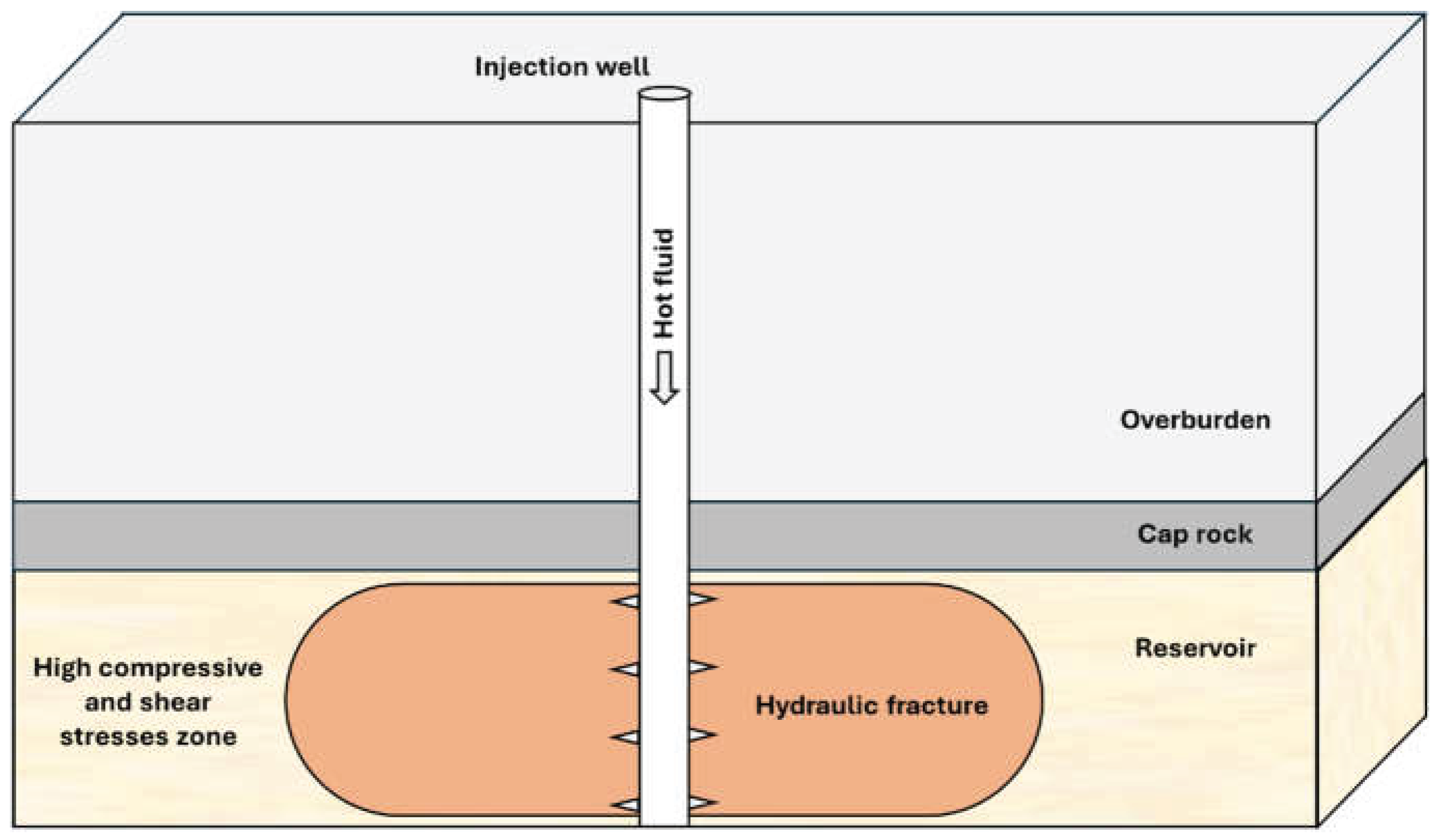
Figure 2.
The fracture is discretized in space and time. Along the fracture boundary, the domain is divided into N straight elements. Element i has a half-length aᵢ and is described in a local coordinate system with tangential axis s and normal axis n. Dₙʲ and Dₛʲ denote the normal and shear displacement discontinuities prescribed on element j, while σₙⁱ and σₛⁱ are the corresponding normal and shear tractions evaluated at the collocation point of element i. The temporal scheme advances a thermo–poroelastic quantity φ(t) in time [17].
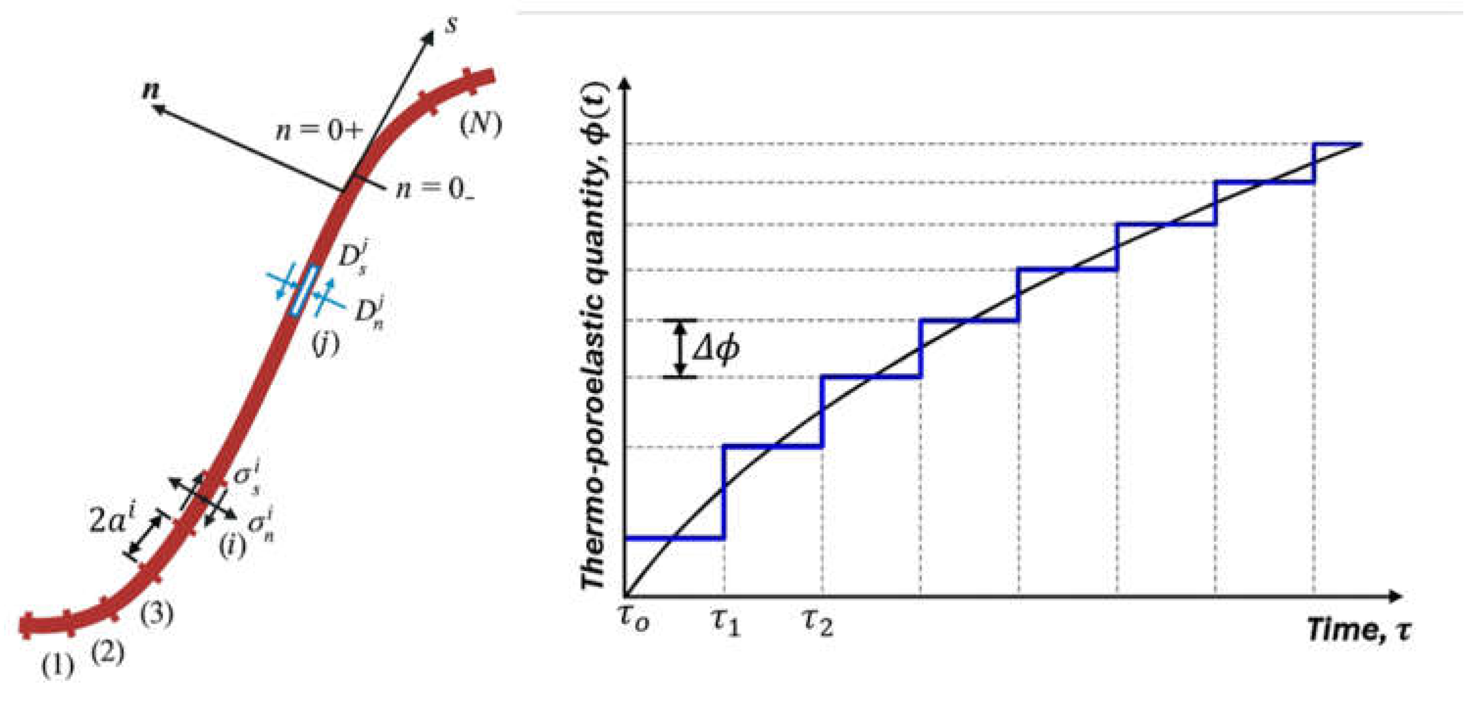
Figure 3.
Figure 3. Fracture propagation modes: Mode I (left) Mode II (middle) and Mode III (right) [17].
Figure 3.
Figure 3. Fracture propagation modes: Mode I (left) Mode II (middle) and Mode III (right) [17].
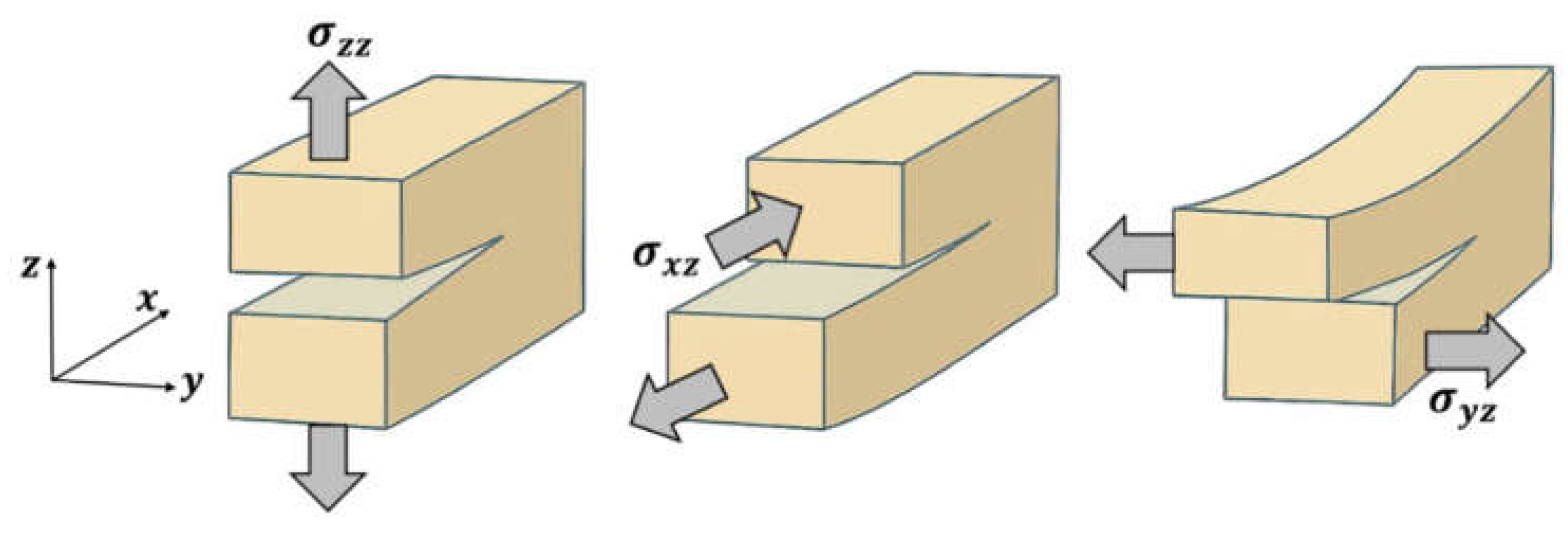
Figure 4.
Schematic diagram of hydraulic fracture [17].
Figure 4.
Schematic diagram of hydraulic fracture [17].
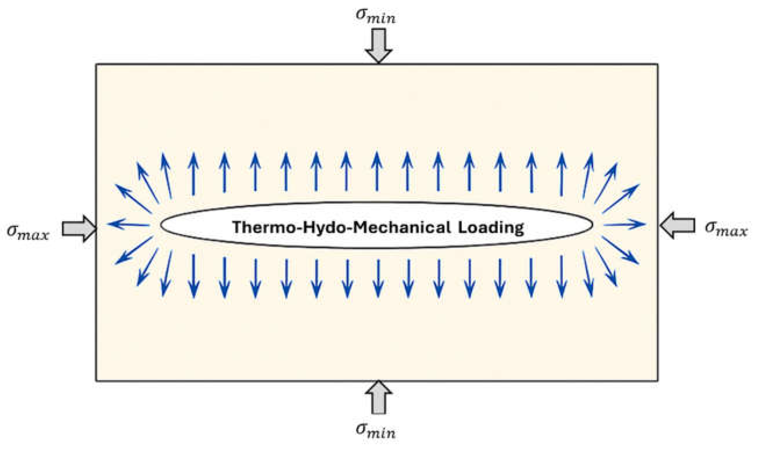
Figure 5.
Aperture evolution during fluid injection (where is temperature difference between hot injection fluid and colder formation).
Figure 5.
Aperture evolution during fluid injection (where is temperature difference between hot injection fluid and colder formation).
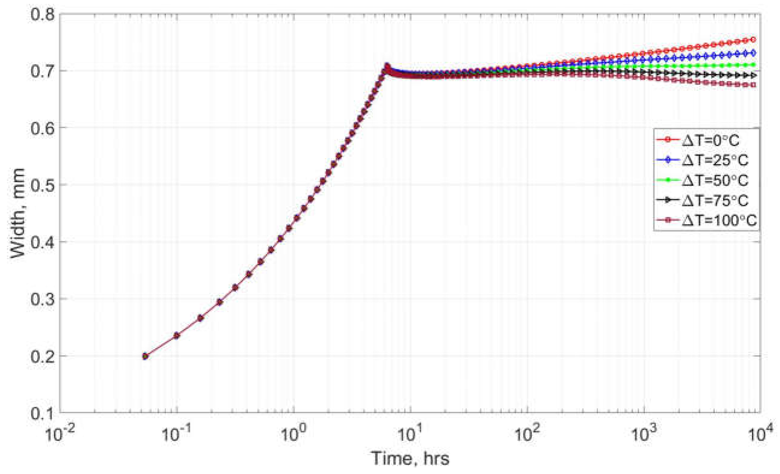
Figure 6.
Aperture distribution at the end fluid injection.
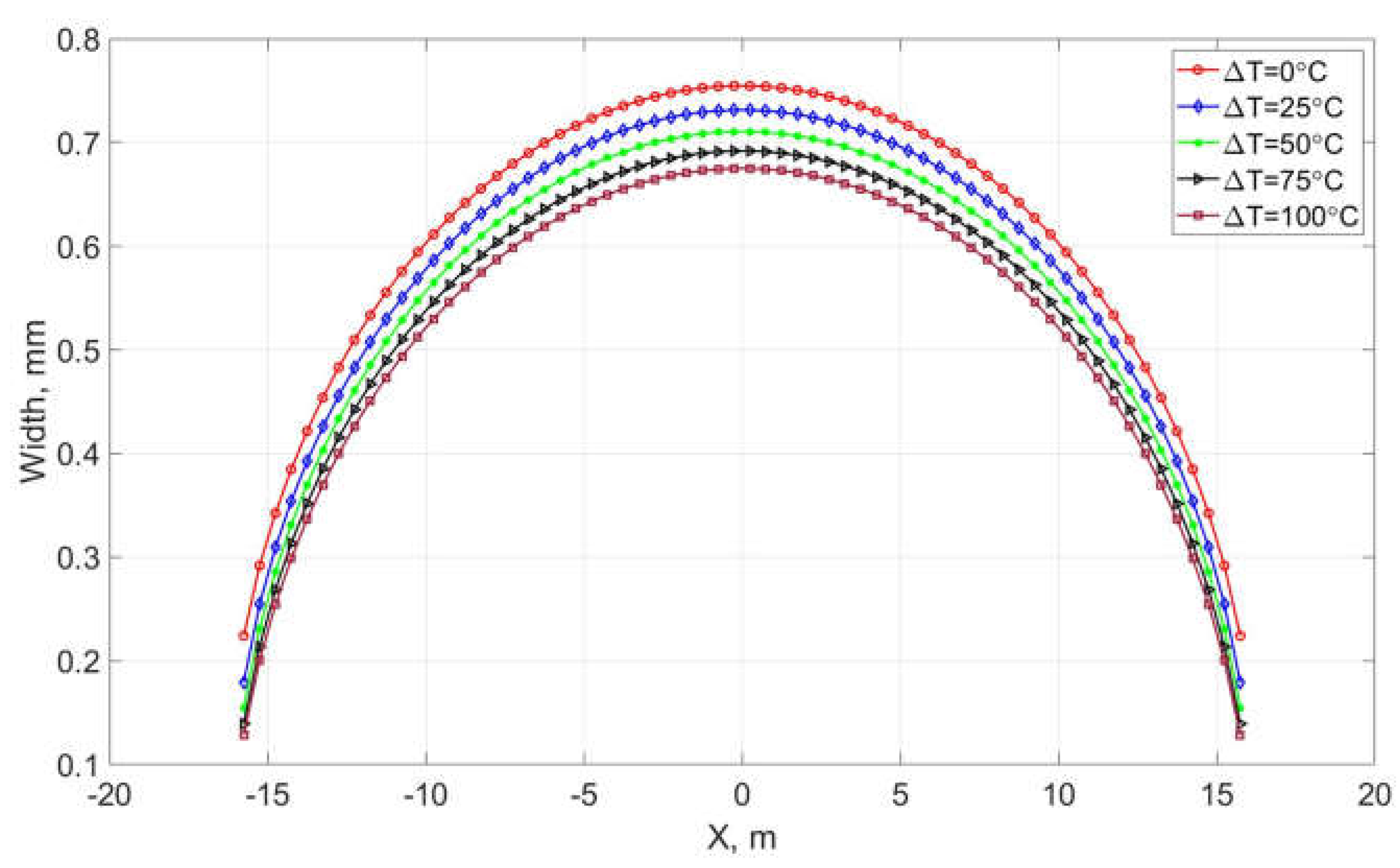
Figure 7.
Minimum principal stress and direction of maximum principal stress at the end of 12-month injection period (A) (B) (C) .
Figure 7.
Minimum principal stress and direction of maximum principal stress at the end of 12-month injection period (A) (B) (C) .
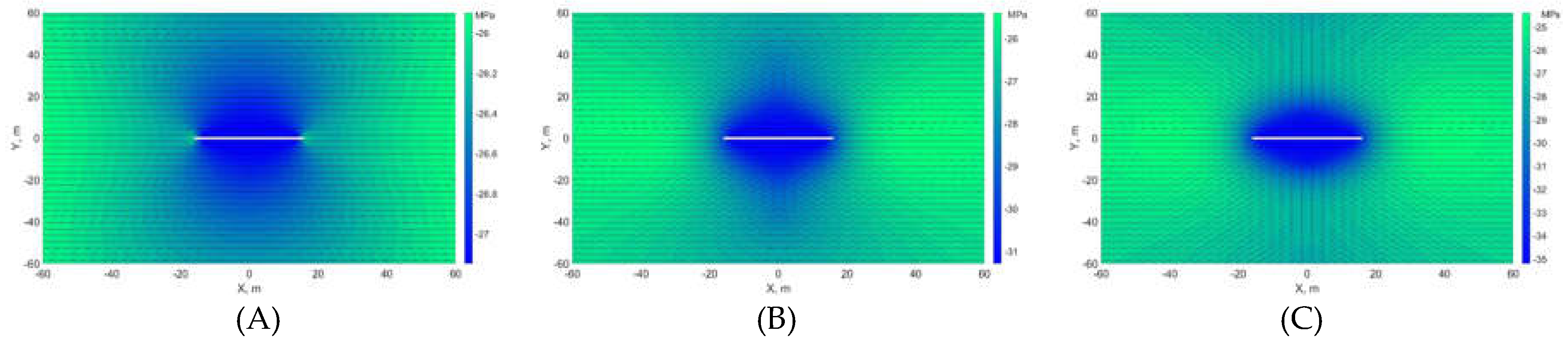
Figure 8.
Change in normal stress in x-direction at the end of 12-month fluid injection period (A) (B) (C) .
Figure 8.
Change in normal stress in x-direction at the end of 12-month fluid injection period (A) (B) (C) .
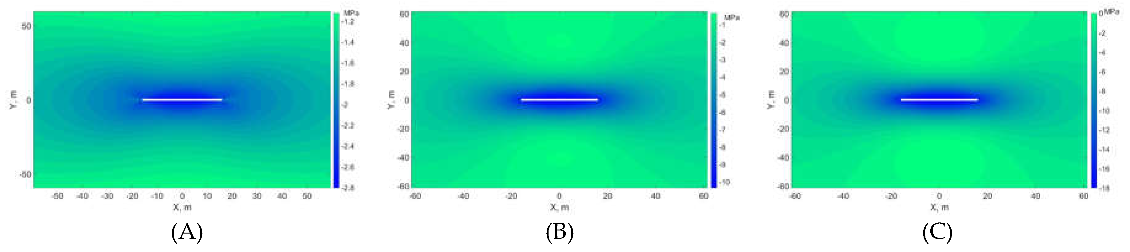
Figure 9.
Change in normal stress in y-direction Δσ_yy at the end of 12-month fluid injection period (A) ΔT=0°C (B) ΔT=50°C (C) ΔT=100°C.
Figure 9.
Change in normal stress in y-direction Δσ_yy at the end of 12-month fluid injection period (A) ΔT=0°C (B) ΔT=50°C (C) ΔT=100°C.
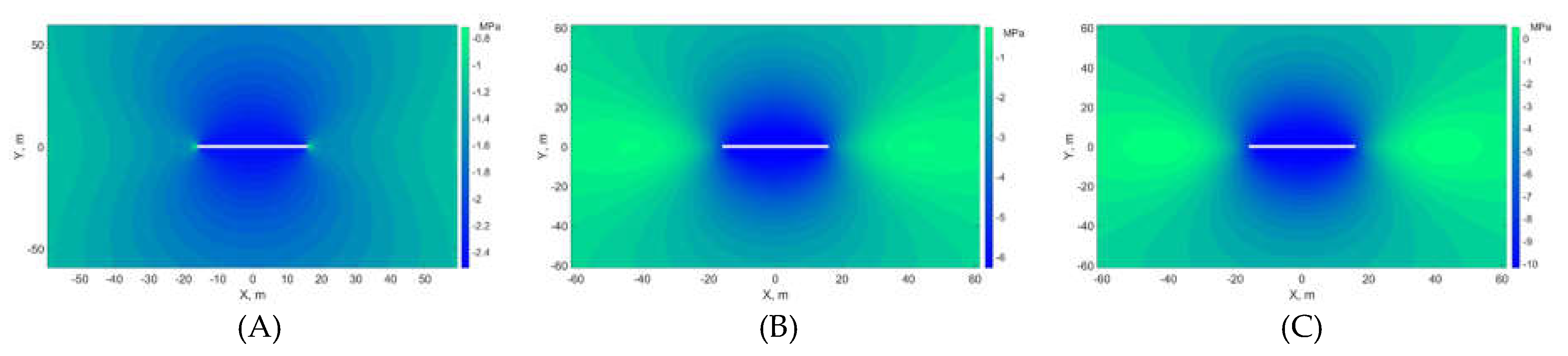
Figure 10.
Shear stress distribution at the end of 12-month fluid injection period (A) (B) (C) .
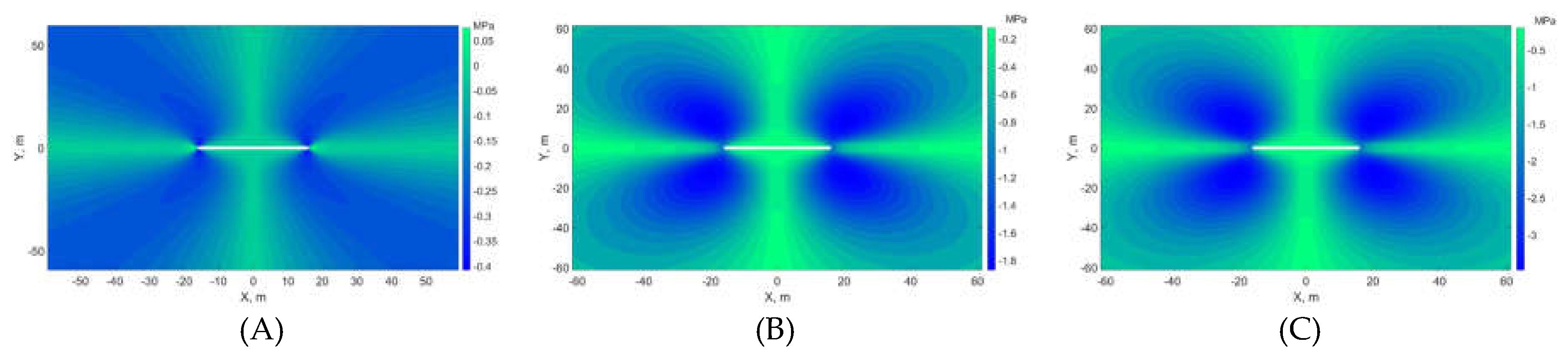
Figure 11.
Change in normal and shear stresses at the end of 12-month hot fluid injection period along line x=1, starting from (1,1) and ending at (1,300) (A) (B) (C) .
Figure 11.
Change in normal and shear stresses at the end of 12-month hot fluid injection period along line x=1, starting from (1,1) and ending at (1,300) (A) (B) (C) .
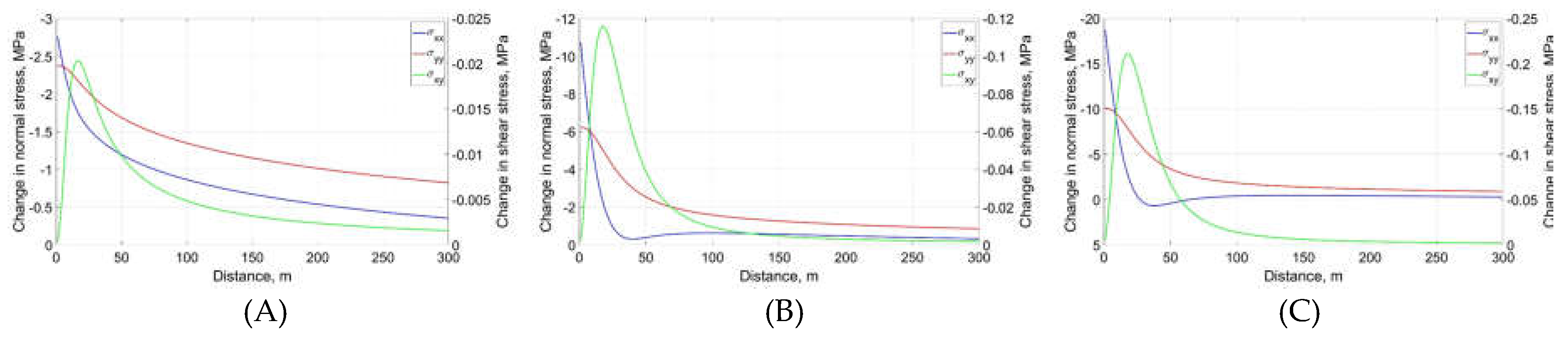
Figure 12.
Minimum and maximum stresses and stress rotation angle at the end of 12-month hot fluid injection period along line x=1, starting from (1,1) and ending at (1, 300) (A) (B) (C) .
Figure 12.
Minimum and maximum stresses and stress rotation angle at the end of 12-month hot fluid injection period along line x=1, starting from (1,1) and ending at (1, 300) (A) (B) (C) .
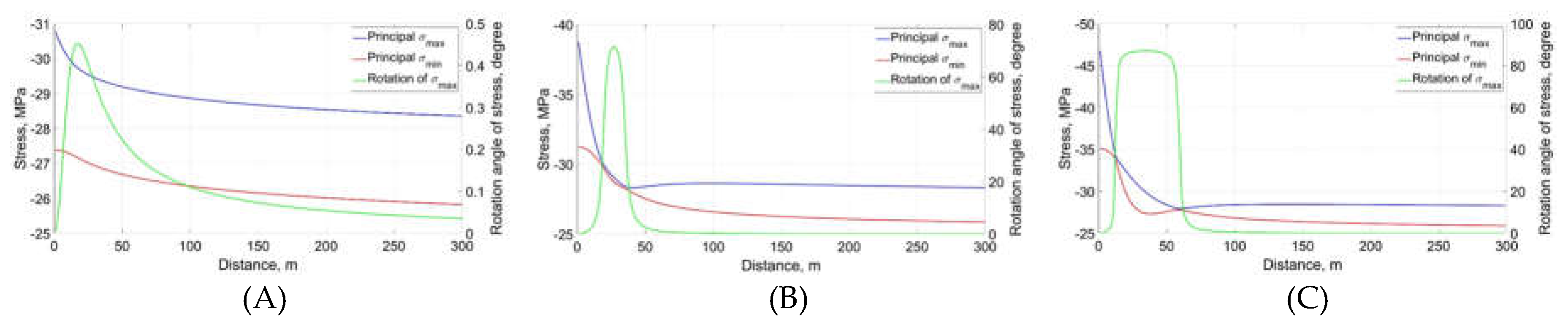
Figure 13.
Change in normal and shear stresses at the end of 12-month hot fluid injection period along line y=1, starting from (1,1) and ending at (300,1) (A) (B) (C) .
Figure 13.
Change in normal and shear stresses at the end of 12-month hot fluid injection period along line y=1, starting from (1,1) and ending at (300,1) (A) (B) (C) .
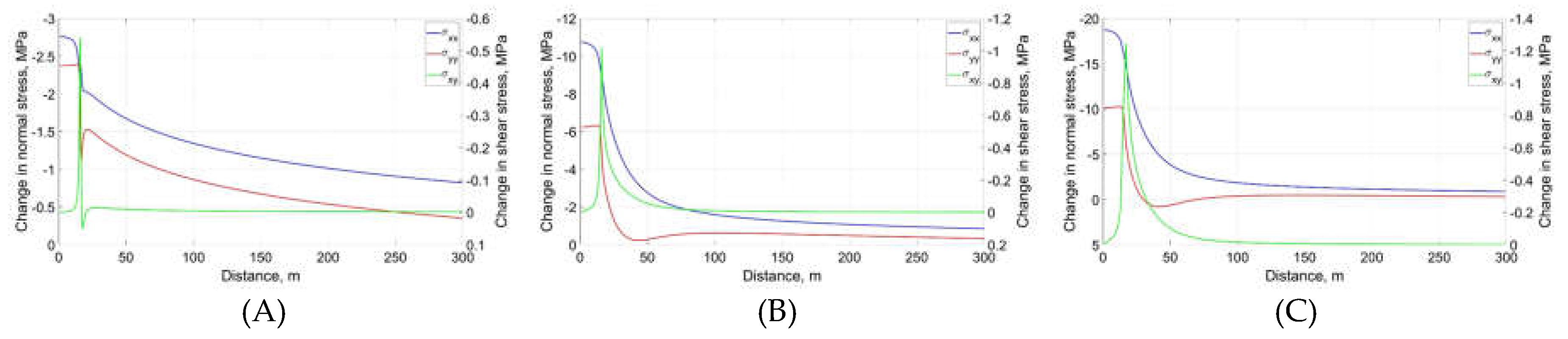
Figure 14.
Minimum and maximum stresses and stress rotation angle at the end of 12-month hot fluid injection period along line y=1, starting from (1,1) and ending at (300,1) (A) (B) (C) .
Figure 14.
Minimum and maximum stresses and stress rotation angle at the end of 12-month hot fluid injection period along line y=1, starting from (1,1) and ending at (300,1) (A) (B) (C) .
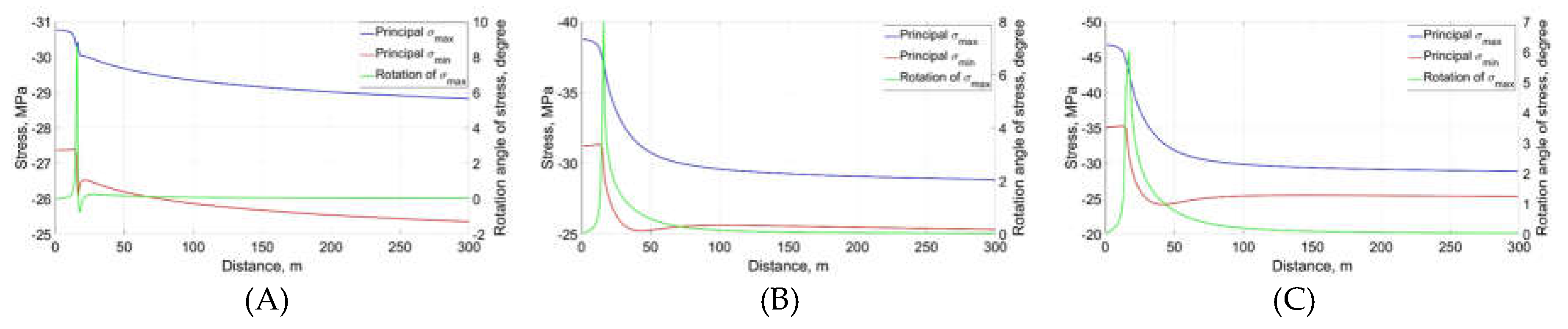
Figure 15.
Increase in temperature distribution at the end of 12-month hot fluid injection period (A) (B) .
Figure 15.
Increase in temperature distribution at the end of 12-month hot fluid injection period (A) (B) .
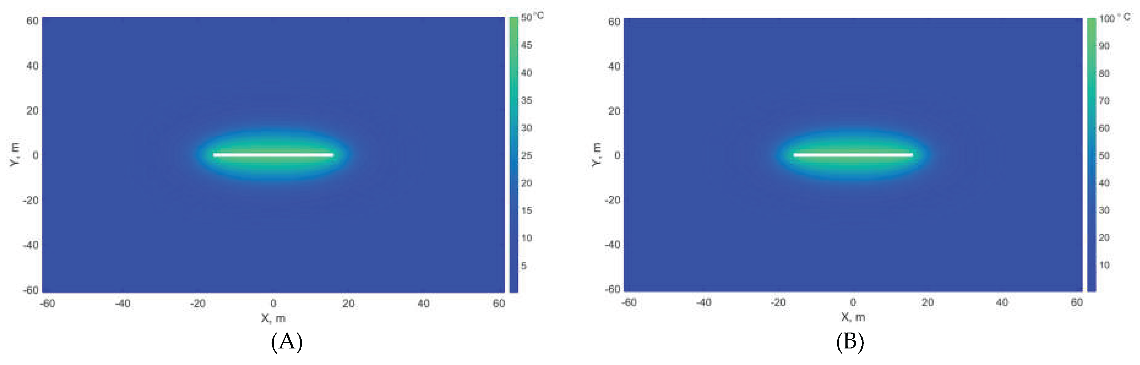

Table 1.
Physical, mechanical, and thermal properties of formation.
Disclaimer/Publisher’s Note: The statements, opinions and data contained in all publications are solely those of the individual author(s) and contributor(s) and not of MDPI and/or the editor(s). MDPI and/or the editor(s) disclaim responsibility for any injury to people or property resulting from any ideas, methods, instructions or products referred to in the content. |
© 2026 by the authors. Licensee MDPI, Basel, Switzerland. This article is an open access article distributed under the terms and conditions of the Creative Commons Attribution (CC BY) license (http://creativecommons.org/licenses/by/4.0/).
Copyright: This open access article is published under a Creative Commons CC BY 4.0 license, which permit the free download, distribution, and reuse, provided that the author and preprint are cited in any reuse.


