The Association Between Soil Sampling and Bait Traps in Wireworm Monitoring

1. Introduction

Agriotes are a genus of click beetles whose larvae are known as “wireworms”. Nine main species of agricultural importance can be found in Europe: Agriotes brevis Candèze, A. lineatus L., A. litigiosus Rossi, A. obscurus L., A. proximus L., A. rufipalpis Brullé, A. sordidus Illiger, A. sputator L., and A. ustulatus Schäller (Elateridae: Elaterinae: Agriotini [1]. They are among the main soil-dwelling pests in Europe and may cause significant damage to a variety of crops, such as maize, potato and sunflower [2,3]. Some of these species are also important in North America [4]. The widespread and often preventive use of insecticides, which is not always justified by the actual presence of damaging populations, can have serious ecological consequences, including biodiversity loss and broader effects on agricultural ecosystems [5,6]. Consequently, accurate monitoring of Agriotes populations is essential for their sustainable and targeted management, with it also helping to reduce pesticide use and adhere to the principles of Integrated Pest Management (IPM) [7].

The main approaches for monitoring Agriotes populations are soil-larval sampling with bait traps [8,9,10], soil samplers, i.e. taking soil cores [11], and pheromone traps [12,13]. Soil sampling has also been evaluated in North America with wireworm species belonging to other genera [14,15]. Pheromone traps are cost-effective tools that are well-suited to large-scale monitoring; they also identify dominant species and predict damage risk, particularly when used over multiple consecutive years [13]. This information results in the identification of the fields where susceptible crops should not be sown, or where larval populations levels should be monitored when susceptible crops will be sown there nevertheless [13]. It has been shown that wireworm monitoring with bait traps can reliably predict the risk of wireworm damage to the subsequent maize crop, and damage thresholds have been pinpointed for Agriotes brevis, A. sordidus and A. ustulatus: 1, 2 and 5 larvae per trap respectively [8].

Bait-trap captures provide an indirect estimate of larval-population levels, although the actual wireworm density remains unknown. Therefore, it would be interesting to assess whether an association exists between capture levels estimated by bait traps in a cultivated field and the field’s actual larval density estimated by soil sampling. It would be useful to establish this association for two reasons:

- damage thresholds could be determined in terms of both average number of wireworms/bait trap and larval density, as estimated with soil coring; wireworm monitoring could thus be carried out successfully, even when soil conditions are unsuitable for bait traps (e.g. when soil is densely covered with cover crops or weeds, and in low temperatures);

- it would provide an insight into wireworm ability to move in soil and reach carbon-dioxide emitting sources (e.g. bait traps).

Therefore, a long-term experiment was conducted to determine whether there was an association between bait-trap and soil-coring monitoring in the same cultivated fields.

2. Materials and Methods

This research was conducted from 1993 to 1999 at numerous sites in Veneto, north-east Italy, and Piedmont, in the north-west.

In Veneto, the sites were located in Venice province: 45.635663° N, 12.599302° E; 45.648662° N, 12.594133° E; 45.599336° N, 12.555930° E, 45.627445° N, 12.938679° E; 45.639238° N, 12.961548° E, 45.639127° N, 12.961960° E, 45.582985° N, 12.707132° E, 45.581330° N, 12.702350° E, 45.587950° N, 12.782453° E; 45.587777° N, 12.779563° E; 45.583169° N, 12.808853° E; 45.606747° N, 12.643118° E; 45.606747° N, 12.643118° E; 45.641279° N, 12.589317° E; 45.662771° N, 12.608012° E; 45.663357° N, 12.604755° E; 45.619919° N, 12.450945° E; and Treviso province: 45.698889° N, 12.614562° E; 45.578401° N, 12.316438° E; 45.578948° N, 12.319900° E; 45.581074° N, 12.311373° E.

In Piedmont, the sites were located in Busano 45.325227° N, 7.827563° E; Poirino 44.896864° N, 7.827563° E; Agliè 45.371644° N, 7.749280°E; Druento 45.127104° N, 7.558307° E; Pertusio 45.345874° N, 7.645953°E; and Lombriasco 44.844388° N, 7.637637° E., with appreciable populations of Agriotes brevis Candeze, A. sordidus Illiger and A. 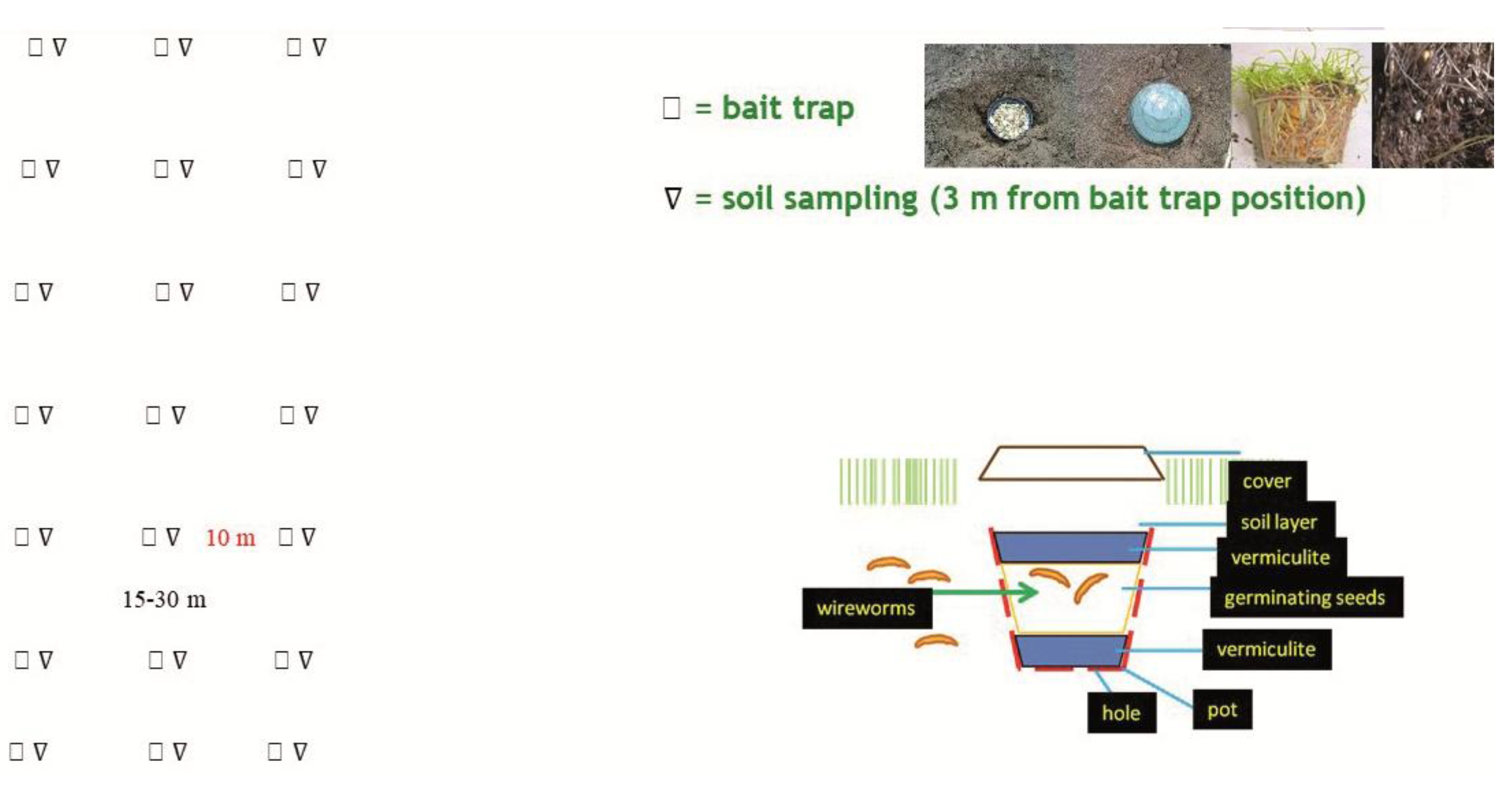ustulatus Schaller being selected based on previous sampling activities and the presence of agronomic risk factors [16]. Within each field, between 12 and 48 sampling points were laid out following a 10 × 15–30 m grid (Figure 1). A bait trap for larvae [8,9] was installed at every point, and a soil core was collected approximately 3 m from the trap’s location. Traps were set on bare soil in late winter or early spring, once ground temperatures at 10 cm below the surface had reached at least 7–8°C, following an established protocol [8]. The traps were retrieved once temperatures had risen and stabilized, which results in most larvae moving towards the upper soil layers after winter.

Soil sampling was performed using a 12-cm diameter manual soil sampler down to a depth of 30 cm. In cases where soil temperature had not yet stabilized, an additional core was taken from 30 to 45–50 cm. Traps remained in the soil for 10 days, occasionally longer if unsuitable weather occurred during the monitoring period [8]. To recover all live and mobile larvae, trap contents were examined manually and then placed in 26-cm Berlese funnels fitted with a 0.5-cm mesh. Samples were allowed to dry for at least 30 days, until two consecutive inspections yielded no new larvae, and all individuals that had fallen into the collecting vials were counted and identified [1]. Soil cores were processed in the same way using 28–30 cm funnels, with a longer drying period of at least 60 days. Whereas soil sampling catches any larvae present in a single core, bait traps attract larvae moving through the soil by emitting carbon dioxide, which wireworms can detect [17].

In the original dataset, each soil-larval sample was linked to its corresponding trap located 3 m away. For the resampling analysis, however, this spatial pairing was deliberately broken, with larval samples and trap captures being randomly reassigned within each field, thus generating a bootstrap dataset free from the inherent spatial dependence of the original design. This bootstrap procedure was repeated 5,000 times, after excluding rows with missing values. For each species, the resulting table summarizes the number and percentage of iterations in which the two detection methods agreed (both detected presence or both detected absence), or disagreed (only one of the two methods detected a presence).

2.1. Statistical Analysis

The statistical analysis was structured in successive and increasingly complex phases to reflect the distributional properties of the data and the biological processes underlying wireworm detection. Analyses addressed both qualitative (presence/absence) and quantitative (counts) relationships between larvae detected in soil cores (SOIL CORES) and larvae captured in bait traps (TRAPS). All analyses were conducted in R Studio (R Core Team, version 4.2.2), and details on model formulations, software implementations and packages are provided in Annexes 1–3.

2.1.1. Exploratory and Descriptive Analyses

Initial exploratory analyses focused on the joint distribution of observations obtained with the two sampling methods. Observations were classified into four categories (absence in both methods, presence in traps only, presence in soil cores only, and concordant presence) and summarized by species and for the entire dataset. Summary statistics (including zero frequency, central tendency, dispersion, skewness, kurtosis, and inequality indices) were computed to characterize data structure and heterogeneity.

2.1.2. Presence/Absence Association Analyses

To assess the agreement between the two detection methods independently of abundance, larval data were first reduced to binary presence/absence information. Contingency tables were constructed for each species and for the pooled dataset. Pearson’s Chi-squared test and Fisher’s Exact test were used to evaluate independence between SOIL CORES and TRAPS, while the Phi coefficient was calculated to quantify the strength of association. To evaluate whether the observed agreement depended on the spatial pairing between soil cores and traps (3 m), a bootstrap procedure was applied. In the bootstrapped datasets, soil-core observations were randomly reassigned to traps within each site, thereby breaking the original spatial pairing while preserving marginal frequencies. Concordance and discordance rates from observed and bootstrapped datasets were then compared to assess the robustness of the association.

2.1.3. Non-Parametric Correlation Analyses

As larval count data were highly skewed and zero-inflated, traditional parametric correlation measures were deemed inappropriate. Non-parametric correlation analyses were therefore used as an intermediate exploratory step. Spearman’s rank correlation coefficient (ρ) and Kendall’s tau (τ) were computed to evaluate monotonic associations between larval counts in soil cores and trap captures for each species. Kendall’s τ was considered particularly suitable given the large number of tied values resulting from frequent zeros. These analyses provided an initial quantitative indication of association strength and guided subsequent modelling steps, but were not intended to fully describe the underlying relationship.

2.1.4. Diagnostic Assessment of Parametric Assumptions

Prior to fitting regression-based models, the suitability of Gaussian assumptions was formally evaluated. Linear regression and ANOVA-type models were initially tested for comparison purposes. Model assumptions were assessed using the Shapiro-Wilk test for normality, the Breusch-Pagan test for heteroscedasticity, and the Durbin-Watson test for autocorrelation; they were applied to raw TRAPS data and to log- and square-root-transformed values. The persistence of non-normality, heteroscedasticity and residual dependence across all transformations demonstrated that standard linear modelling frameworks were inappropriate for these data, motivating the adoption of count-based models.

2.1.5. Count-Based Regression Models

Given the discrete nature of the data, generalized linear models (GLMs) for counts were subsequently fitted. A Poisson GLM was considered as the simplest formulation, followed by quasi-Poisson and negative binomial models to account for overdispersion. Overdispersion was evaluated using dispersion statistics and residual diagnostics. As preliminary analyses revealed a large excess of zero observations, models explicitly accounting for zero inflation were then fitted. These included hurdle negative binomial models and zero-inflated Poisson (ZIP) and zero-inflated negative binomial (ZINB) models. Zero-inflated models allow zeros to arise from two distinct processes: (i) true absence of larvae and (ii) non-detection despite presence, which is particularly relevant in ecological sampling contexts. For comparison purposes, generalized least squares (GLS) models with heteroscedastic variance structures and linear mixed-effects models (LMMs) were also fitted, although these models do not explicitly address zero inflation.

2.1.6. Model Selection

Model selection followed an information-theoretic approach. For likelihood-based models, Akaike’s Information Criterion (AIC) and Bayesian Information Criterion (BIC) were used to compare competing models, with lower values indicating better support after accounting for model complexity. Differences in AIC were used to assess relative model performance. For quasi-likelihood models, which do not provide a true likelihood, model adequacy was evaluated using dispersion parameters and residual diagnostics rather than information criteria. Model comparisons were first conducted on the pooled dataset and subsequently repeated for each species separately to assess species-specific differences in model performance.

2.1.7. Model Validation and Performance Assessment

The final selected models were validated through a comprehensive assessment of goodness-of-fit and predictive performance. Residual diagnostics included inspection of Pearson and deviance residuals, evaluation of remaining overdispersion, and assessment of fitted versus observed values. For zero-inflated and hurdle models, observed and predicted zero frequencies were compared to evaluate the adequacy of the zero-generating component. Predictive performance was further quantified using root mean square error (RMSE), median absolute deviation (MAD), and correlation between observed and model-predicted trap counts. Incidence Rate Ratios (IRR) were calculated to quantify the effect of larval abundance in soil cores on expected trap captures.

3. Results

Across all three Agriotes species, soil cores showed a high proportion of zero counts (86%–94%), whereas traps exhibited substantially lower zero percentages (37%–53%) (Table 1). As a consequence, mean abundances were consistently higher in traps than in soil cores, particularly for A. ustulatus, where the median abundance in traps was 1, compared to 0 in soil cores. Measures of variability, including interquartile range (IQR) and median absolute deviation (MAD), were negligible in soil cores, highlighting limited variation in soil samples, whereas traps showed greater dispersion, consistent with their lower zero-inflation. Gini coefficients were generally high across all datasets, suggesting that individuals were concentrated in a limited number of samples. Positive skewness and high kurtosis values further indicate strongly right-skewed and leptokurtic distributions, particularly in traps, reflecting infrequent but high-abundance events.

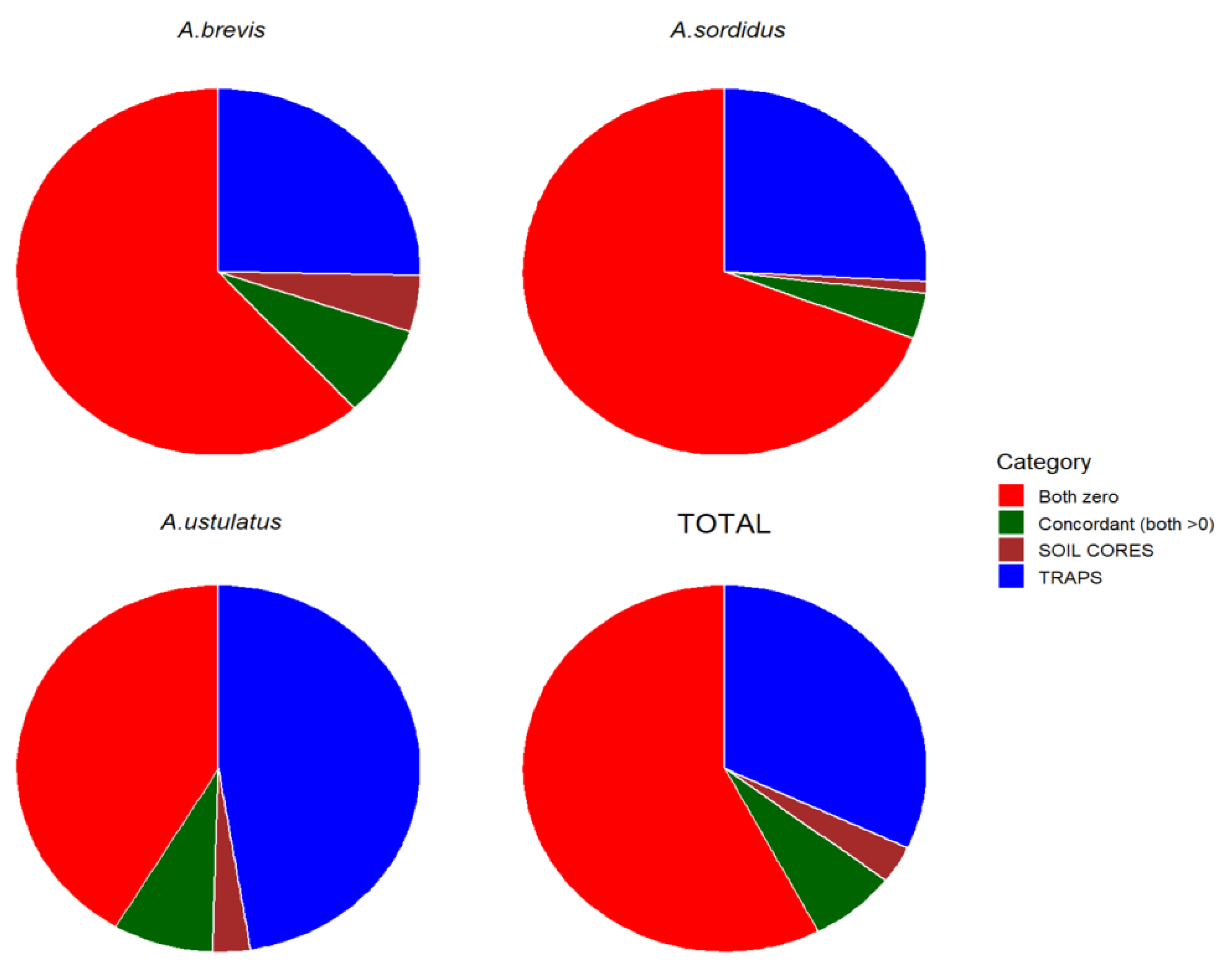
In all species (Figure 2), the dominant outcome is the concurrent absence of detections in both soil cores and bait traps (red), which accounts for roughly two-thirds to three-quarters of all observations, depending on the species. This confirms that most sampling points did not detect any larval activity with either method. Samples positive only in TRAPS (blue) constitute the second most frequent category, generally accounting for about one-quarter to one-third of observations. This result suggests that bait traps are more sensitive than soil cores. Concordant detections (green) are relatively uncommon (below 10%) while detections restricted to SOIL CORES (brown) consistently represent the smallest proportion, usually only a small percentage of samples.

A. ustulatus displayed the most distinct pattern of the three species studied. Its proportion of trap-only detections was substantially higher than for A. brevis and A. sordidus. In contrast, A. brevis and A. sordidus showed more similar and balanced distributions across categories. This divergence highlights that bait traps are particularly effective for A. ustulatus, amplifying the difference in detection efficiency between the two methods for this species.

The contingency analysis (Table 2) evaluates the agreement between the presence/absence of wireworms (Agriotes spp.) in the soil. The spatial pairing (3 m) allowed a direct comparison to be made between the two detection methods based on binary (presence/absence) data.

For A. brevis, the statistical tests (Pearson’s Chi-squared and Fisher’s Exact) yielded highly significant results (P < 0.001), indicating a strong and consistent association between larval presence in the soil cores and trap captures. The high proportion of concordant observations suggests that the two sampling methods are largely complementary and provide coherent information on the spatial distribution of A. brevis populations.

A similarly strong relationship was observed for A. sordidus, with the statistical tests again highly significant (P < 0.001). In contrast, A. ustulatus exhibited a weaker, though still statistically significant relationship between the two methods (P < 0.05 for Chi-squared and Fisher’s tests). This suggests that while a general correspondence exists between larvae in soil cores and larvae captured by traps, the association is more variable or inconsistent. The strong correspondence observed for A. brevis and A. sordidus supports the reliability of bait traps as indicators of underground larval populations.

The comparison between the observed and bootstrapped datasets (Table 3) reveals major differences in the strength and stability of the relationship between larval presence in soil cores and captures in bait traps for the three Agriotes species. In the field dataset, each soil core (larval sampling point) was spatially paired with a trap located 3 m away, while in the bootstrapped dataset, by contrast, the association between larvae in soil cores and bait traps was randomized within each site, thereby removing the original spatial pairing and allowing the evaluation of whether the observed correspondence could occur by chance.

For A. brevis and A. sordidus, both the observed and bootstrapped data showed a high level of concordance between the two detection methods. In A. brevis, 69.75% of field pairs were concordant (both presence or both absence), compared to 68.49% under random reassociation. Similarly, A. sordidus showed 73.15% of concordant cases in the field and 70.83% in the bootstrapped dataset. The close similarity between observed and randomized results suggests that the strong correspondence between detections is robust and not simply a product of the specific spatial pairing.

In contrast, A. ustulatus exhibited a weaker and less spatially dependent relationship. The proportion of concordant cases was 49.55% in the field data and 51.82% in the bootstrapped dataset.

The similarity between observed and randomized associations suggests that the 3 m spatial pairing does not strengthen the correspondence between soil cores and traps, indicating that trap effectiveness is likely driven by processes operating at a spatial scale smaller than 3 m, or by non-spatial factors.

Note that this analysis is based on presence/absence data, thus providing an initial evaluation of the consistency between the two monitoring methods. In the following analyses, the number of individuals captured will also be examined to further assess the quantitative relationship between larval density quantified with the two methods.

To evaluate the association between the two detection methods, the joint distributions of observations referring to the presence of larvae in the soil and trap catches were analyzed.

Table 4 reports the contingency table aggregated over the entire dataset. The data show that sites with larvae present in soil cores exhibit a much higher frequency of positive captures in traps than sites without larvae.

The contingency table also reveals that the probability of obtaining a positive trap capture is considerably higher when larvae are present in the soil (78/115, 67.8%) compared with when larvae are absent (359/1004, 35.7%). This indicates that trap captures tend to reflect, at least partially, the underlying presence of larvae in the soil, although a substantial fraction of trap positives also occurs where no larvae with soil sampling were detected.

The Chi-square test (Table 5) indicates a highly significant association between the two detection methods (χ² = 65.2, p < 0.001), rejecting the hypothesis of independence. The Phi coefficient (0.36) denotes a moderate association, implying that the two variables are related but not strongly correlated. From an applied perspective, this suggests that the presence of larvae in the soil substantially increases the probability of detecting larvae in traps, although trap captures also depend on additional ecological or methodological factors not directly measured here.

Given the complex nature of the TRAP data revealed by initial diagnostic tests, traditional parametric approaches like Pearson’s correlation were deemed inappropriate due to violated distributional assumptions. The analytical approach was structured in progressive phases, starting with non-parametric methods and advancing to more sophisticated models. Non-parametric techniques, specifically Spearman’s rank correlation coefficient (ρ) and Kendall’s tau (τ) tests, were applied to explore non-linear relationships and detect monotonic associations without constraints of linearity or specific distributional forms. These methods proved insightful in uncovering potential patterns that might have remained hidden using only traditional parametric methods (Table 6).

Kendall’s τ was particularly suitable for the zero-inflated datasets, being less affected by tied ranks common in observations with many identical values (zeros). The resulting non-parametric correlation coefficients (Table 6) consistently indicated positive associations between larval counts in soil cores and captures in bait traps across all Agriotes species, with varying strengths of relationships.

While these non-parametric methods provided a preliminary interpretative framework and guided initial hypotheses, they did not allow for explicit modeling of the observed phenomenon’s intrinsic complexity, particularly the pronounced zero inflation. This limitation highlighted the need for more advanced modelling techniques in subsequent analysis phases.

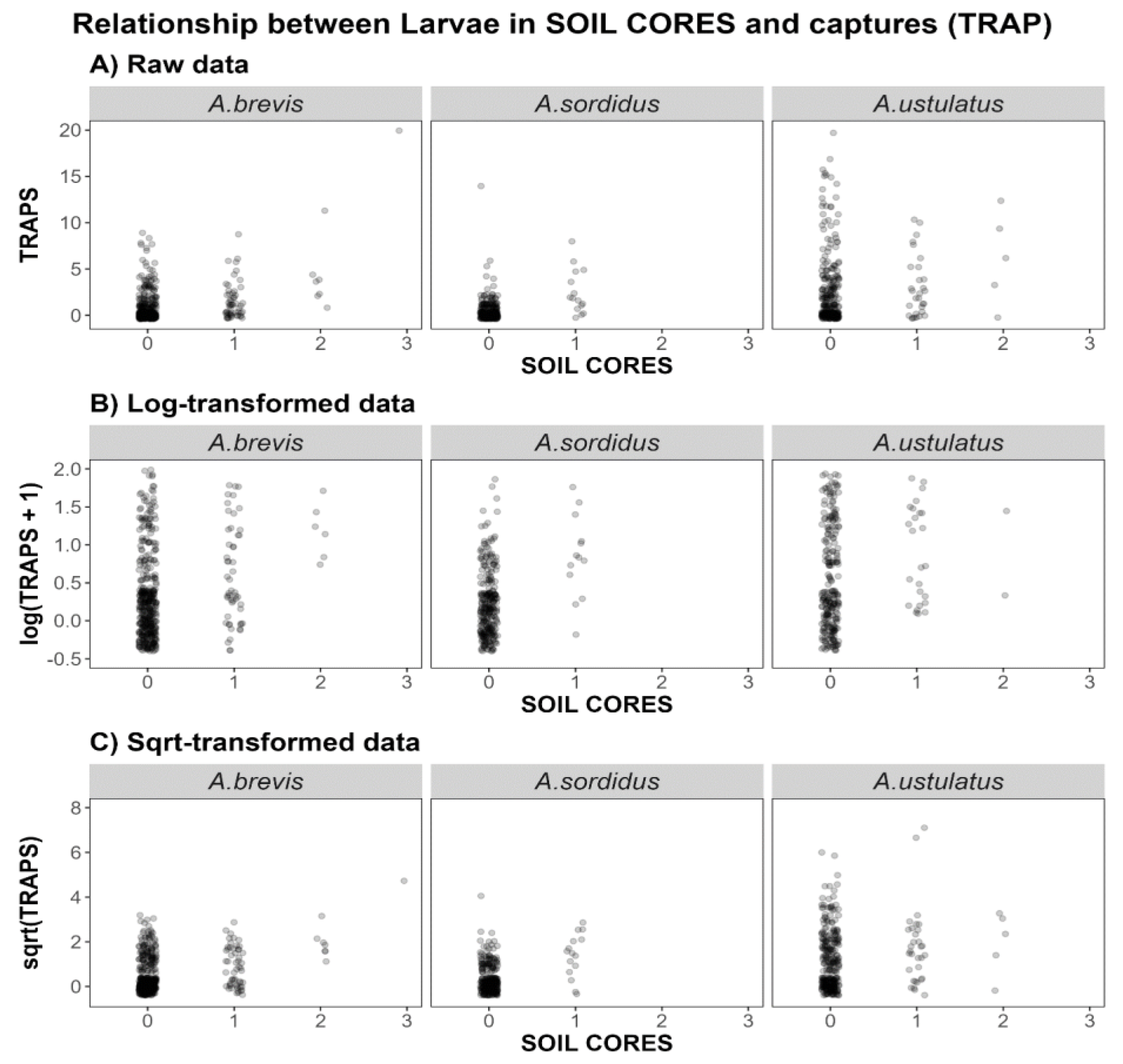
A visual examination of the scatter plots (Figure 3), which illustrate the relationship between Agriotes larvae detected in soil cores and those captured in bait traps, reveals a clear methodological issue: data distributions are markedly non-normal across all larval abundance categories and for each of the three Agriotes species. The majority of observations is concentrated at low larval counts, with a high frequency of zero values, indicating that both soil sampling and bait traps often resulted in no detection of individuals.

Despite the data transformations (logarithmic and square-root), the overall pattern remains largely unchanged, with evident clustering near the origin and a limited range of higher values. These distributions suggest that the relationship between the two methods is weak and strongly zero-inflated, implying that linear assumptions may not fully capture the underlying ecological processes or detection probabilities. This deviation from normality is primarily driven by pronounced zero inflation. A substantial clustering of data points occurs at the origin (SOIL CORES = 0, TRAPS = 0), as clearly shown by the geometric jitter. In addition, the non-zero values display strong right-skewness: most captures are concentrated at very low larvae counts, with a long tail toward infrequent but high trap catches.

These distributional features violate the fundamental assumptions of standard parametric statistical approaches such as Analysis of Variance (ANOVA) and linear regression. Even without formal normality testing, the visual evidence alone clearly indicates that applying conventional parametric models would lead to unreliable or invalid inferences.

To further investigate the relationship between larval counts in soil and trap captures, a Generalized Linear Model (GLM) was initially tested using a Gaussian error distribution. However, diagnostic tests clearly indicated that the assumptions underlying ANOVA-type models were not met. Table 7 presents the results of diagnostic tests performed on the TRAPS data and its transformations (log(TRAPS+1) and sqrt(TRAPS)). Three key statistical tests were employed to assess the assumptions required in linear regression models: the Shapiro-Wilk test for normality; the Breusch-Pagan test for heteroscedasticity; and the Durbin-Watson test for autocorrelation in residuals. The Shapiro-Wilk test yielded p-values < 0.001 for all forms of the data, indicating significant deviations from normality. These findings collectively suggest that the TRAPS data, in both their original and transformed states, violate key assumptions of standard linear regression models. The persistence of these issues across different data transformations indicates that simple transformations are insufficient to address the underlying complexities of the data structure.

It must be pointed out that although the fitted regression models produced statistically significant coefficients (data not shown), these results must be interpreted with caution, as the violation of the model assumptions invalidates the inferential reliability of standard F-tests.

To adequately address these data characteristics, analysis was conducted using modeling frameworks specifically designed for count data. Given the complex nature of the TRAPS data revealed by diagnostic tests, more sophisticated modeling techniques were employed. In particular, the use of Generalized Linear Models (GLMs) with non-Gaussian error distribution was explored.

Generalized Linear Models, specifically Poisson and Negative Binomial regressions, were initially considered as they can adapt to non-normal and skewed distributions, common in ecological count data. These models provide a more flexible framework compared to standard linear regression, allowing for a more appropriate representation of the data structure.

However, because a pronounced zero inflation was observed, a further extension of the modeling approach was adopted. Consequently, Zero-Inflated models were tested, specifically Zero-Inflated Poisson (ZIP) and Zero-Inflated Negative Binomial (ZINB) models. The adoption of Zero-Inflated models is particularly relevant in ecological contexts. These models allow for the simultaneous representation of two distinct processes that could lead to zero observations:

• True absence: cases where larvae in both soil-core captures and trap captures are genuinely absent from the sampled area;
• Non-detection: instances where individuals are present but not observed due to various factors such as sampling limitations or organism behavior.

This dual-process modeling approach generally provides a more ecologically meaningful interpretation of the present data. It acknowledges that zeros in our dataset may arise from different underlying mechanisms, thereby offering a more accurate representation of the ecological phenomena under study. The implementation of these advanced modeling techniques not only addresses the statistical challenges identified in our initial diagnostic tests, but also aligns more closely with the ecological realities of TRAPS data collection and interpretation.

When the various statistical models used to describe the relationship between the number of Agriotes larvae captured in bait traps (TRAPS) and the number of larvae detected through soil sampling (SOIL CORES) were compared (Table 8), the Zero-inflated Negative Binomial (ZINB) model yielded the lowest AIC and BIC values (2932 and 2977 respectively). This indicates that the ZINB model provides the most appropriate representation of the data structure among the models evaluated.

The Poisson model exhibited substantial overdispersion (dispersion parameter = 5.07), indicating a clear violation of the equidispersion assumption. In contrast, the Negative Binomial model achieved a dispersion value close to unity (≈1.1), confirming its improved ability to account for extra-Poisson variability.

The ZINB model also produced the highest coefficients of determination (marginal R² = 0.21; conditional R² = 0.799), suggesting that fixed effects explain a limited proportion of the observed variability, whereas random effects and/or latent zero-inflation processes account for a substantial share of the total variance. This pattern indicates the presence of important unmeasured factors or latent ecological and sampling processes influencing larval detection, beyond the directly observed explanatory variables.

The zero-inflated models (ZINB, ZIP, and Hurdle) explicitly estimated the zero-inflation parameter, with the Hurdle model showing the highest zero-inflation probability (0.557) and the ZINB model the lowest (0.098). This suggests that the ZINB model provides a more balanced explanation for both zero and non-zero counts. In contrast, simpler models such as the linear model (LM), generalized least squares (GLS), and Poisson GLM showed much higher AIC and BIC values, indicating poorer fit. These simpler models also exhibited signs of overdispersion, confirming that they fail to account for the complex distributional features of the data, particularly the overabundance of zeros and the non-linear relationship between the two measurement methods.

In practical terms, the ZINB model suggests that only a small fraction (≈10%) of the zeros correspond to true absences of insects, while the remaining zeros can be explained by random variation in sampling. The ZIP model, on the other hand, overestimates the number of structural zeros (≈30%), leading to a less accurate description of the data. The Hurdle model assumes an even stronger zero component (≈56%), but because it forces all zeros to come from a separate process, it can overstate the biological meaning of zeros. Overall, the evidence supports the view that most zeros are sampling zeros, not structural absences. They are consistent with the ecological context of insect presence data. Furthermore, the lower proportion is biologically realistic, since both soil cores and traps are spatially aggregated and influenced by environmental heterogeneity; complete absences are rare but possible.

Since the analysis of the entire dataset revealed that the ZIP (Zero-Inflated Poisson) and ZINB (Zero-Inflated Negative Binomial) models offered the best compromise between simplicity and data fit, these models were subsequently tested on individual datasets for each of the three species under consideration: A. brevis, A. sordidus and A. ustulatus. This approach allowed for a more detailed examination of how these models perform when applied to species-specific data, potentially revealing any variations in model effectiveness across the three Agriotes species.

For A. brevis, the Zero-Inflated Poisson (ZIP) model estimated a moderate level of zero inflation (≈0.34) with no evidence of overdispersion (dispersion = 1.00). By contrast, the Zero-Inflated Negative Binomial (ZINB) model reduced the estimated zero inflation to approximately 0.10 and accounted for mild overdispersion (dispersion = 1.22). The lower AIC (1077.88 vs. 1114.61) and BIC (1098.82 vs. 1131.36) for the ZINB model indicate a better fit to the data.

For A. sordidus, the ZIP model suggested a low zero-inflation probability (≈0.17) and no overdispersion. The ZINB model, however, nearly eliminated zero inflation (≈1.5×10⁻⁸) while capturing substantial overdispersion (dispersion = 1.83). Correspondingly, the reduced AIC (516.01 vs. 529.84) and BIC (534.50 vs. 544.63) further support the superior performance of the ZINB model.

In the case of A. ustulatus, the ZIP model indicated moderate zero inflation (≈0.30) with no overdispersion. The ZINB model again reduced zero inflation (≈0.12) and accounted for slight overdispersion (dispersion = 1.14), with considerably lower AIC (1343.53 vs. 1663.91) and BIC (1362.60 vs. 1679.17), demonstrating improved model fit. The relatively modest predictive performance observed for this species may be partly explained. This could lead to an overrepresentation of captured larvae relative to larval density in the soil, thus weakening the correspondence between trap catches and larval counts.

These results suggest that larval counts across all three species are characterized by both excess zeros and overdispersion. The ZINB models consistently provided a more accurate representation of the data by simultaneously accounting for these two features.

Figure 4. ZINB Model of Larval Abundance in SOIL CORES vs. captures in TRAPS in A. ustulatus, A. brevis and A. sordidus. The scatter plot shows the relationship between larval counts in soil cores (x-axis) and captures in bait traps (y-axis). Species-specific trends are indicated by colored fitted lines.

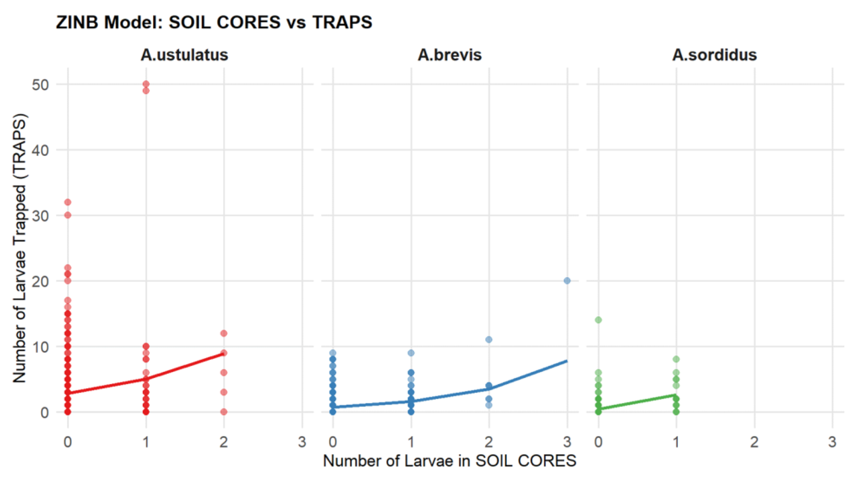
Figure 4. ZINB Model of Larval Abundance in SOIL CORES vs. captures in TRAPS in A. ustulatus, A. brevis and A. sordidus. The scatter plot shows the relationship between larval counts in soil cores (x-axis) and captures in bait traps (y-axis). Species-specific trends are indicated by colored fitted lines.

Trap catches exhibit a positive but highly heterogeneous relationship with the number of larvae detected in soil cores. The fitted ZINB curves show increasing expected trap captures with higher larval densities, yet the magnitude and variability of this response differ substantially among species, in agreement with Table 9.

For A. ustulatus, trap captures are markedly higher and more dispersed than for the other species. Maximum trap values exceed 40 individuals, even when soil cores contain 0–1 larvae, generating a vertical spread of more than one order of magnitude at the lowest soil densities. The model reflects this behavior: the ZINB estimates a dispersion parameter of 1.14 and reduces the zero-inflation probability from 0.30 (ZIP) to 0.12 (ZINB), while improving fit dramatically (AIC reduction of 320 points). Quantitatively, the predicted trap mean increases from about 6–8 individuals when 1 larva is detected in soil to more than 20 individuals for 3–4 larvae. These values confirm that A. ustulatus is by far the species with the strongest and least proportional trap response.

For A. brevis, trap catches rarely exceed 8–10 individuals, and the ZINB curve rises more proportionally with soil counts. The ZINB model reports a dispersion of 1.22 and a low zero-inflation value (0.10), indicating that most variability is accounted for by the negative binomial component. AIC decreases from 1098.22 (ZIP) to 1080.53 (ZINB). The predicted mean trap catches increase from approximately 2 individuals at low soil counts to 6–7 individuals when soil cores contain 4–5 larvae, illustrating a moderate but consistent relationship.

For A. sordidus, trap counts are generally low, with most observations below 5 individuals and a very shallow response curve. Despite the low counts, the species exhibits strong overdispersion (dispersion = 1.83), and the ZINB model nearly eliminates zero inflation. The improvement from ZIP to ZINB (AIC 529.84 to 516.01) confirms that overdispersion, rather than excess zeros, drives model performance. Quantitatively, predicted trap means increase only modestly, from 0.5–1.0 individuals at low soil densities to 2–3 individuals at the highest observed larval counts.

Overall, the quantitative patterns indicate that A. ustulatus differs sharply from the other species, displaying the highest trap responsiveness, the strongest deviations from proportionality, and the most extreme trap counts. A. brevis shows moderate but consistent increases in trap captures with soil larvae, while A. sordidus exhibits the weakest and least variable relationship. These species-specific differences highlight the distinct behavioral responses to bait traps and help explain the contrasting model fits observed across species.

Table 10. Incidence Rate Ratios (IRR) for larval counts in soil cores and predictive performance metrics of zero-inflated negative binomial (ZINB) models for three click beetle species (Agriotes ustulatus, A. brevis and A. sordidus). Reported statistics include Pearson’s correlation coefficient, root mean square error (RMSE) and mean absolute deviation (MAD). IRR represents the multiplicative change in the expected number of larvae captured by bait traps for each additional larva detected in a soil core. RMSE is defined as the square root of the mean squared difference between observed and predicted values and reflects predictive accuracy with greater sensitivity to large errors, whereas MAD represents the mean of the absolute differences between observed and predicted values, and provides a robust measure of average prediction error that is less influenced by extreme values.

INSECT	IRR (SOIL CORES)	Correlation (Predicted vs Observed)	RMSE	MAD
A. ustulatus	1.76	0.148	5.82	3.49
A. brevis	2.22	0.472	1.68	1.10
A. sordidus	5.79	0.355	1.24	0.72

Table 10. Incidence Rate Ratios (IRR) for larval counts in soil cores and predictive performance metrics of zero-inflated negative binomial (ZINB) models for three click beetle species (Agriotes ustulatus, A. brevis and A. sordidus). Reported statistics include Pearson’s correlation coefficient, root mean square error (RMSE) and mean absolute deviation (MAD). IRR represents the multiplicative change in the expected number of larvae captured by bait traps for each additional larva detected in a soil core. RMSE is defined as the square root of the mean squared difference between observed and predicted values and reflects predictive accuracy with greater sensitivity to large errors, whereas MAD represents the mean of the absolute differences between observed and predicted values, and provides a robust measure of average prediction error that is less influenced by extreme values.

INSECT	IRR (SOIL CORES)	Correlation (Predicted vs Observed)	RMSE	MAD
A. ustulatus	1.76	0.148	5.82	3.49
A. brevis	2.22	0.472	1.68	1.10
A. sordidus	5.79	0.355	1.24	0.72

Larval abundance in soil cores was positively associated with larval captures in bait traps for all three species, as revealed by Zero-Inflated Negative Binomial models. The IRR indicated that each additional larva in soil cores increased expected trap captures by 76%, 122% and 579% for A. ustulatus, A. brevis and A. sordidus respectively. Model fit, assessed as the Pearson correlation between predicted and observed trap captures, was low for A. ustulatus (r = 0.148) and moderate both for A. brevis (r = 0.472) and for A. sordidus (r = 0.355). RMSE and MAD values further illustrate model performance: lower values for A. brevis and A. sordidus (RMSE: 1.68, 1.24; MAD: 1.10, 0.72) indicate more accurate predictions, whereas higher values for A. ustulatus (RMSE: 5.82; MAD: 3.49) reflect greater variability and less precise predictive ability. These results confirm that larval counts in soil cores are a significant predictor of trap captures, with species-specific differences in effect strength and predictive reliability, suggesting that bait traps can serve as a practical proxy for estimating larval abundance in soil, particularly for species showing stronger soil core/trap relationships.

4. Discussion

Across all species, soil cores yielded a high proportion of zero counts, reflecting frequent absence of individuals in the sampled soil. In contrast, while traps exhibited markedly lower zero percentages, indicating higher detection efficiency for active wireworms, thus mean and median abundances were consistently higher in traps compared to soil cores, particularly for A. ustulatus, where the median abundance in traps was 1, compared to 0 in soil cores (Table 1, Table 2 and Table 3, and Figure 2). Measures of variability showed that individuals were concentrated in a limited number of samples, indicating that wireworms of the studied species have primarily an aggregated distribution, while in a previous study [11] this distribution occurred but it was not prevalent.

A. ustulatus displayed the highest proportion of trap-only detections indicating a stronger behavioral response to the food-based attractant or a higher movement capacity that increases the probability of finding the bait trap for an individual wireworm.

Our findings demonstrate that the relationship between the number of Agriotes larvae in soil cores and captures in bait traps is statistically significant but only moderate in strength, indicating that both methods reflect the same wireworm distribution in the soil. Significant Chi-square and Phi statistics confirm an overall correspondence between methods; however, this concordance largely results from the simultaneous absence of insects in both traps and soil samples. Once double-zero observations are excluded, discrepancies become more evident, suggesting that positive detections are not necessarily shared between the two sampling techniques.

The non-parametric correlation analyses support this conclusion. Both Spearman’s ρ and Kendall’s τ revealed positive but modest associations between larval densities evaluated with the two methods. The correlations were strongest for A. brevis and A. sordidus, whereas A. ustulatus exhibited a markedly weaker relationship.

From a statistical perspective, the dataset was characterized by pronounced zero inflation and overdispersion, violating the assumptions of Gaussian or Poisson error structures. Tests of normality and homoscedasticity, along with residual diagnostics, consistently indicated that simple data transformations were insufficient to satisfy model assumptions. Such patterns are typical in field entomological studies, where spatial aggregation, heterogeneous microhabitats, and variable detection probabilities generate a high proportion of zeros and long-tailed count distributions. These properties justify the use of models capable of distinguishing between true absences and sampling zeros.

Model comparison identified the Zero-Inflated Negative Binomial (ZINB) model as the most appropriate framework for describing the relationship between larval counts and trap captures. ZINB models consistently produced the lowest AIC and BIC values, effectively accommodating both excess zeros and overdispersion, and yielding the highest conditional R². This suggests that a dual-process model—one describing true counts and another accounting for structural zeros—best represents the observed data. Biologically, this implies that many zero observations likely reflect non-detections rather than true absences. In contrast, Zero-Inflated Poisson models tended to overestimate the zero component, while simpler Poisson or linear models failed to capture the observed data dispersion. It might also indicate the need to consider other factors, or to further investigate the processes that generate many zeros in the dataset.

The improvement achieved by ZINB models highlights the importance of integrating ecological understanding with statistical modeling. It is known that larval populations of Agriotes spp. can be patchily distributed in soil [11,14,18]. This is probably originated by the females’ behavior: female click beetles lay clusters of several eggs that cause an initial concentration of small larvae [19,20], while female movements to suitable egg-laying sites are triggered by plant volatiles and/or pheromones [21,22,23,24,25], driving a further egg/larval concentration for all of the three species studied. This explanation is supported by the results of i) Furlan and Burgio [11], who demonstrated that the distribution of young/small A. ustulatus larvae was more aggregated than the spatial distribution for old last-instar larvae; and ii) Doane [14], who demonstrated that the small larvae of Ctenicera destructor were much more aggregated than the large ones. While growing, the larvae move from oviposition sites and disperse, reducing population aggregation. This may, or may not, result in a Poisson distribution. These results indicate that, under random sampling, the probability of obtaining zero captures is high, whereas the likelihood of detecting additional wireworms in the vicinity of a soil core or bait trap where larvae were recorded is higher than in areas with zero-larvae samples. This pattern is further supported by the contingency tables (Table 2 and Table 4), which show the predominance of zero–zero observations alongside a higher proportion of positive trap captures when larvae were present in soil cores. Moderate but significant non-parametric correlations (Table 6) and the scatter plots (Figure 3) also reflect this tendency, with a clustering of zeros and a tendency toward co-occurrence of positive detections, consistent across the three Agriotes species.

Bait trap capture potential is significantly higher than soil sampling (Table 11), thus the probability of finding zero-capture points on the same soil plot is lower when bait traps are used. This is due to carbon dioxide emitted by the germinating seeds and seedlings in the bait traps that attracts the larvae over some days, while in the core only the larvae present at that precise moment can be caught. Monitoring with bait traps simply exploits the natural mechanisms that enable larvae to find seeds and seedlings to feed on. The traps tend to capture higher numbers of larvae even when larval densities in the soil are low, thereby weakening the statistical relationship between the two detection methods.

Since the relationship between the number of Agriotes larvae in soil cores and captures in bait traps is statistically significant, we can convert the established wireworm damage thresholds in maize based on the average number of wireworms/bait trap [8] into the average number of wireworms/soil sample and the relative density in the soil (Table 11). The thresholds set with bait traps for maize result in soil sampling thresholds that range between 15 to 20 larvae/m². No peer review papers have reported thresholds based on soil sampling from fields, although some “grey” journals have reported indications without any clear description of the methods applied. According to Le Nail [26], wireworm populations can cause conspicuous plant damage to maize, sugar beet and tobacco when they exceed the threshold of 20 larvae/m². The thresholds for potato and cereal crops have been established at 30 larvae/m². Said thresholds do not refer to one species, but to wireworms generically; however, Le Nail [26] does describe A. lineatus, A. obscurus and A. sputator as the main species in the area studied. Although Suss [27] provides a description of the methods adopted, it is incomplete and not very detailed. Details, however, include the sampling of 12 cm diameter cores, as in the present study, 15 cm deep, with 10 samples taken diagonally per plot, or every 10 m, according to indications by Khinkin [28]. No details are provided about the larvae-extraction method, although it appears to be manual, or how damage to plants and yield is assessed. The author reports that up to 12–15 larvae per square meter of wireworms did not lead to appreciable plant losses or a decrease in yield. However, with populations between 28 and 46 larvae per square meter, high damage was observed. The author refers generically to wireworm larvae without having determined the species being researched. Subsequent research [29] established that A. sordidus and A. brevis are the prevalent wireworms in corn rotations in the Po Valley (A. ustulatus was also prevalent in the eastern part); research by Suss [27] was mainly conducted here, as well.

More than one century ago (1914–1922), Roebuck [30] took from five to twelve soil samples per field (mainly ploughed-up pastures). The size of the soil samples was 0.052 m² (about 23 x 23 cm) and 30 cm in depth. Soil was crumbled and sifted to recover the wireworms. Although no larvae identification is given and it is possible that wireworm density could be overestimated, the damage thresholds suggested are close to the numbers found in the present study. Negligible wireworm damage to all the crops was found below 12.4 larvae/m². Low wireworm damage to most of the crops was observed from 12.4 to 24.7 larvae/m² while from 24.7 to 49.4 larvae/m² was tolerably safe for cereals, broadcast crops and established plants. Beans, as later papers confirmed, were a tolerably safe crop where wireworms are numerous. Regarding cereals, oats proved to be more tolerant to wireworms than winter wheat and barley, which was the most susceptible.

Our discoveries have enabled us to achieve the first goal of this research, i.e. to estimate a bait-trap catch value from soil sampling so that a risk assessment based on soil- sampling catches can be performed and vice versa.

For research and practical purposes, it is also possible to suggest the minimum number of soil samples to be taken for a reliable estimate of wireworm populations. When looking for population levels around the thresholds (Table 11), Furlan and Burgio [11] found that 16 (A. brevis) and 13 (A. ustulatus) are the minimum number of soil cores to be taken for an error of approximately 25%. For higher precision, more than 40 soil cores are needed.

As for wireworms’ ability to move through soil and reach carbon-dioxide emitting sources, results highlight that the potential of bait traps (with germinating seeds) to attract and catch wireworms was 5 to 25 times higher than the potential of soil sampling. Soil cores give an instant snapshot of larval presence at monitoring time, while bait traps estimate how many larvae in the surrounding soil can reach the carbon-dioxide emitting source in 10 days: 1/15 of larvae in a square meter for A. brevis; 1/10 of larvae in a square meter for A. sordidus; and 1/3 of larvae in a square meter for A. ustulatus, which means that theoretically 30% of the larvae in the 55 cm around the trap can be captured. Since only part of the larvae are in the feeding phase [19,20], this means that a significant proportion of the active larvae in a 55 cm radius may enter the trap. Some larvae from greater distances may enter the trap by chance.

5. Conclusions

This long-term study shows that a monitoring method to assess wireworm population levels is always available. Although developed for Agriotes spp., the statistical framework presented here is not species-specific and may be adapted to other insect pests and agroecosystems. Its application could support a more extensive interpretation of monitoring data in situations characterized by low detection rates and heterogeneous field conditions.

As for the practical implications of the results, a range of IPM packages can be implemented once the risk of wireworm damage has been assessed with agronomic factor evaluation [16,31] and adult pheromone traps [13], and the most suitable wireworm soil-monitoring method has identified whether a wireworm population exceeds the threshold. These packages comprise tolerant crops and genotypes within a crop [32], e.g. bioactive cover crops [33,34], entomopathogens [35] and naturally derived ingredients [36], as well as other agronomic strategies and tools [37].