Submitted:
31 December 2025
Posted:
31 December 2025
You are already at the latest version
Abstract
Traditional reliability engineering paradigms, originally designed to prevent physical component failures, are facing a fundamental crisis when applied to today's soft-ware-intensive and autonomous systems. In critical domains like aerospace, the dom-inant risks no longer stem from the aleatory uncertainty of hardware breakdowns, but from the deep epistemic uncertainty inherent in complex systematic interactions and non-deterministic algorithms. This paper reviews the historical evolution of reliability engineering, tracing the progression through the Statistical, Physics-of-Failure, and Prognostics eras. It argues that while these failure-centric frameworks perfected the management of predictable risks, they are structurally inadequate for the "unknown unknowns" of modern complexity. To address this methodological vacuum, this study advocates for an imperative shift towards a fourth paradigm: the Resilience Era. Grounded in the principles of Safety-II, this approach redefines the engineering objec-tive from simply minimizing failure rates to ensuring mission success and functional endurance under uncertainty. The paper introduces Uncertainty Control (UC) as the strategic successor to Uncertainty Quantification (UQ), proposing that safety must be architected through behavioral constraints rather than prediction alone. Finally, the paper proposes a new professional identity for the practitioner: the system resilience architect, tasked with designing adaptive architectures that ensure safety in an era of incomplete knowledge.
Keywords:
reliability engineering
; uncertainty quantification
; resilience engineering
; uncertainty control
1. Introduction
1.1. The Growth of Complexity in Safety-Critical Systems
The landscape of modern engineering is being reshaped by a profound and accelerating increase in system complexity. This is most evident in safety-critical domains such as aerospace, automotive, and maritime industries, where a fundamental transition is underway from systems defined by their physical and mechanical properties to those defined by their software, connectivity, and increasingly, their autonomy [1,2]. This evolution is not merely a linear extrapolation of past trends but represents a step-change in the nature of the systems that engineers must design, analyze, and certify.
A prime example of the system with the above-mentioned new properties is the emergence of electric Vertical Take-Off and Landing (eVTOL) aircraft for Urban Air Mobility (UAM). Unlike traditional aircraft, eVTOLs are characterized by highly integrated distributed electric propulsion (DEP) systems, where aerodynamic forces, structural loads, and flight control logic are deeply and non-linearly coupled [3]. To achieve the necessary performance, stability, safety and reliability in dynamic urban environments, these vehicles rely on advanced, often non-deterministic control algorithms, such as Model Predictive Control (MPC) or even machine learning (ML)-based controllers [4,5]. This trend is also existing in modern civil aircraft whose avionics system has been upgraded to Integrated Modular Avionics (IMA) architectures. IMA transforms the aircraft into a software-defined platform, where multiple functions of differing criticalities share a common set of computational resources, making system safety contingent upon the correct and non-interfering interaction of countless software partitions [6,7]. Likewise, the progression from static, gain-scheduled flight controllers to adaptive flight control systems introduces a new level of performance alongside significant challenges in verification and predictability [8,9].
The distinctive feature of these modern systems is their high degree of integration and interactivity. They are no longer loose collections of independent subsystems but are tightly coupled architectures where a state change or a fault in one domain can propagate instantaneously and non-linearly across the entire platform, leading to system-level hazards that are unable to foresee through traditional decomposition analysis [10,11]. Furthermore, the introduction of autonomy fundamentally alters the human-machine relationship. Operators are moving from direct manual control to a supervisory role, creating new classes of risks related to mode confusion, loss of situational awareness, and the opacity of autonomous decision-making processes [12,13].
Consequently, the defining characteristic of these modern systems is not just their scale, but the profound uncertainty inherent in their design, operation, and environment. This uncertainty stems from the size of possible system state-space, the unpredictable nature of machine learning algorithms, the complexity of software-hardware-human interactions, and the highly dynamic environments in which they must operate[14] . As these systems become ubiquitous, the engineering community faces a critical challenge: the existing reliability and safety assurance frameworks, developed for a simpler, more deterministic era, are proven to be inadequate for managing the risks posed by those uncertainty factors.
1.2. The Emerging Crisis of Traditional Reliability Paradigms
The historical paradigms of reliability engineering, including statistical methods, physics modeling and prognostic-based approach, share a unifying philosophical foundation: they are fundamentally failure-centric. This worldview posits that system safety is primarily a function of component reliability. The core assumption is that accidents and system failures are the result of a chain of cascading or concurrent component faults—a broken part, a software bug, or a sensor that stops working [15]. Consequently, the primary engineering objective has been to understand, predict, and prevent these component failures. This philosophy is formally recognized in safety science as "Safety-I," which defines safety as the absence of accidents and incidents [16].
This failure-centric perspective is deeply embedded in the classical tools of reliability and safety evaluation. Techniques like Failure Modes and Effects Analysis (FMEA) and Fault Tree Analysis (FTA) are built upon a reductionist premise: that by exhaustively analyzing the ways individual components can fail and tracing their consequences, one can understand and mitigate system-level risk [17]. The underlying logic is that if all components are made sufficiently reliable, then the whole system will be safe. This can be conceptually represented as:
where represents the union of all possible sets. In this model, which assumes that system accidents can be decomposed into a sum or combination of component failures, has been remarkably successful for decades in improving the safety of mechanical and electro‐mechanical systems. However, this fundamental assumption is now in direct conflict with the reality of modern complex systems.
The main crisis facing traditional reliability is the increasing prevalence of accidents in which no component has failed according to its individual failure criteria. In the highly integrated or software-intensive systems, catastrophic failures are increasingly caused not by broken parts, but by unsafe interactions among components that are all functioning exactly as designed [10]. These are known as emergent failure, i.e., system-level properties, that cannot be predicted by analyzing components in isolation. The accidents involving the Boeing 737 MAX Maneuvering Characteristics Augmentation System (MCAS) serve as a tragic example. According to National Transportation Safety Board (NTSB) investigation, the individual components were operating as specified, but their collective behavior, orchestrated by software and driven by unexpected environmental inputs, created a hazardous system state [18]. This demonstrates that in modern systems, system failure has shifted from physical components to intellectual design involving the requirements, the control logic, and the assumptions about the operational environment. The comparison of traditional and systemic accident causality is listed in Table 1.
The rise of interactional accidents has created a methodological crisis for traditional reliability engineering. A dangerous gap now exists between the systemic nature of safety in modern platforms and the component-focused tools used to evaluate it. For example, FMEA, by focusing on the effects of individual component failures, is structurally incapable of identifying hazards that arise from unsafe interactions between multiple, non-failed components. Although FTA can model combinations of events, it struggles when the root "events" are not component failures but flawed requirements, complex software logic, or incorrect assumptions about human behavior [19]. The crisis, therefore, is a methodological vacuum between the complex systems we are building and the methods we use for guaranteeing their safety. This necessitates a re-define for the paradigm of reliability engineering, shifting the focus from preventing component failures to controlling the systemic behaviors and uncertainties that lead to hazardous states.
1.3. The Shifting Nature of Uncertainty: From Aleatory to Epistemic
The crisis facing traditional reliability paradigms is not merely a matter of scale, but a fundamental shift in the very nature of the uncertainty that engineers must confront. For decades, the discipline achieved success by mastering the management of aleatory uncertainty. However, the complex, software-defined modern systems are increasingly dominated by epistemic uncertainty [20].
- Aleatory uncertainty
It refers to the inherent, irreducible randomness or variability in a physical system or its environment. Often termed "stochastic uncertainty" or "variability," it represents the natural fluctuations that persist even with perfect knowledge of the system [21]. Classic examples in aerospace include microscopic variations in material fatigue properties, atmospheric turbulence, and manufacturing tolerances within an acceptable range. The defining characteristic of aleatory uncertainty is that, given sufficient data, it can be accurately described by a probability distribution, allowing its impact to be quantified with statistical confidence.
- Epistemic uncertainty
It refers to uncertainty stemming from a lack of knowledge on the part of the observer or modeler. Often termed "cognitive uncertainty" or "reducible uncertainty," it represents a deficit in our understanding that could, in principle, be reduced by gathering more data, developing better models, or gaining more experience [22].
Hence, the total uncertainty in any prediction about a system's behavior is a combination of both. A simplified conceptual model can be expressed as:
where is the true system output, is the established imperfect computer model, represents inputs with inherent randomness, represents model parameters we are unsure about, is the model error and represents the error of all other noise.
Traditional reliability engineering excelled because its primary focus was on characterizing the aleatory terms through extensive testing and statistical analysis by assuming the epistemic terms were negligible or could be managed. However, this assumption is completely violated for the modern complex systems, where epistemic uncertainty is no longer a secondary factor but is now the dominant, and most dangerous source of risk. This dominance arises from several interconnected sources as follows.
- Model uncertainty: as systems like eVTOL operate in novel flight regimes (e.g., transition flight in urban canyons), the physics-based simulation models used for their design become less reliable. The discrepancy between the model and reality grows, representing a significant form of epistemic uncertainty [23].
- Algorithmic uncertainty: the behavior of advanced control algorithms, especially those based on AI/ML, introduces a new form of epistemic uncertainty. For a deep neural network, we lack the complete "knowledge" to predict its output for every possible input, particularly for out-of-distribution scenarios not seen during training [24,25].
- Operational uncertainty: for entirely new operational concepts like Urban Air Mobility (UAM), there is no historical data to build probabilistic models of the environment. This "zero-sample" problem—where we lack knowledge of traffic densities, weather patterns in urban microclimates, or novel human-machine interaction failure modes—is a pure form of epistemic uncertainty [26].
This fundamental shifting nature of uncertainty is not merely an academic observation. It is being actively addressed and codified within the aerospace industry's most critical safety standards. The evolution from SAE ARP4754A to ARP4754B provides direct evidence of this change. The standard's deliberate replacement of the term "unintended function" with "unintended behavior" is a landmark philosophical revolution. An "unintended function" implies a discrete, solvable design error. In contrast, an "unintended behavior" is defined as an "unexpected operation of integrated aircraft systems" that can arise even when all components are functioning as specified [27]. This acknowledges that safety is no longer just about the reliability of individual parts but is an emergent property of the system's interactions—a problem deeply rooted in epistemic uncertainty about those interactions.
To address this new reality, SAE ARP4761A places greater emphasis on specific analytical techniques designed to systemic and interactional risks that FMEA/FTA might miss [28]. Key methods that are now central to the safety process for complex systems include: Cascading Effects Analysis (CEA), Common Cause Analysis (CCA) and Investigation of Unintended Behaviors. These methods tell an industry-wide acknowledgment that the primary threat is no longer just the predictable randomness of component failures, but the epistemic uncertainty surrounding the emergent behavior of the system.
1.4. The Necessity of Change in Uncertainty Management Process
Uncertainty management process consists of uncertainty identification, uncertainty quantification and uncertainty control. For traditional systems where risk was primarily driven by the aleatory uncertainty of component failures, the key task was uncertainty quantification, as the influencing factors were easy to be identified (e.g., material fatigue, electronic part failure) and their relationships could be modeled (e.g., via fault trees or stochastic process). The uncertainty quantification helps engineers to determine the effects created by those factors, given sufficient data [29]. The primary output of this paradigm was a calculated risk metric, such as a probability of failure, which informed design decisions.
However, for the modern system, this traditional paradigm reaches its limits, because the factors influencing safety and reliability have become not only more numerous but also qualitatively different. Key influencing factors are now often difficult to identify totally, the coupling relationships between them are non-linear and difficult to model. Consequently, their effects are often impossible to quantify with high confidence [30]. So, we propose, when a system's behavior under uncertainty can no longer be precisely identified and quantified a priori, the only viable strategy is to control its behavior to stay on the right track during operation [31].
This review argues that to ensure the safety of complex systems, the reliability engineering paradigm must undergo an imperative shift, from a philosophy focused on the passive assessment of Uncertainty Quantification (UQ) to one centered on the active practice of Uncertainty Control (UC). This is not an abandonment of quantification but a re-contextualization of it. UQ remains a critical input, but it is no longer the end goal. The primary objective becomes the design and implementation of mechanisms that provide a generalized form of control over the system's behavior in the face of uncertainty. As articulated by recent work in autonomous systems safety, this term "control" is broad and multi-faceted, including but not limited to: continuous monitoring of operational parameters against defined safety boundaries [32], real-time analysis of system state trends to anticipate divergences from safe operation [33] and architecting predefined recovery strategies or dynamic adjustment mechanisms when encountering unexpected states [34].
As is shown in Figure 1, this shift reframes the ultimate engineering objective from achieving reliability (the prevention of component failures under quantifiable uncertainty) to engineering resilience (the system's capacity to succeed by actively controlling its behavior under uncertain conditions) [35]. In this paper, we will proceed to substantiate this idea by examining the limits of the old paradigm, detailing the foundations of the new UC paradigm, and exploring its implications for the future of the engineering profession.
The discipline of reliability engineering has not been static; rather, it has undergone an accretive evolution, with each new paradigm building upon the last to address increasingly complex challenges. The first three major eras—Statistical, Physics-of-Failure, and Prognostics—represent a multi-decade effort to master the risks associated with component and subsystem failures, primarily driven by aleatory uncertainty. This section will trace this historical layering, detailing how each stage added a new level of proactive capability while retaining the essential tools of the past. By doing so, it will build a compelling argument for why this mature, component-focused philosophy, while still necessary, is no longer sufficient. It has reached its conceptual boundary, creating the imperative for an emerging fourth paradigm—Resilience—which envelops the previous stages to address the systemic, interaction-driven uncertainties for which they were not designed. The main characteristics of the paradigm in each era are listed in Table 2.
1.5. The Organization of This Article
The remainder of this paper is structured to trace the evolutionary trajectory of reliability engineering through four distinct paradigms. Section 2 reviews the Statistical Era, focusing on empirical modeling of component failures under aleatory uncertainty using probability theory. Section 3 discusses the Physics-of-Failure Era, which shifts the focus to "white-box" causal mechanisms to design reliability into physical components. Section 4 examines the Prognostics Era, highlighting the transition toward dynamic, real-time health management and Remaining Useful Life (RUL) prediction via data-driven and hybrid approaches. Section 5 establishes the core argument for the Resilience Era, proposing a strategic shift from Uncertainty Quantification (UQ) to Uncertainty Control (UC). It details the philosophy of operating under deep epistemic uncertainty and introduces key methodologies—Systems Theoretic Process Analysis (STPA) and Run-Time Assurance (RTA)—as the architectural pillars for ensuring mission success. Finally, Section 6 summarizes the study and outlines the future outlook for this discipline.
2. The Statistical Era: Reliability as an Empirical Science
2.1. Core Philosophy: Treating Failure as a Black-Box Stochastic Process
Reliability engineering as a formal discipline emerged in 1950s, primarily driven by the urgent need to address the unacceptably high failure rates of increasingly complex military electronics and aerospace systems [36]. The foundational paradigm of this period was rooted in probability theory and mathematical statistics, treating the complex system as an analytical "black box." The core philosophy was that failures, regardless of their intricate physical origins, could be modeled as stochastic events occurring over time. The primary objective was not to understand the root causes of failure but to empirically characterize the failure behavior of a large population of components based on extensive test or operational field data.
This approach was a direct and practical response to the dominant challenge of that time: aleatory uncertainty, the inherent and irreducible randomness in material properties, manufacturing processes, and operational loads [21]. By assuming failures were random variables, engineers could use statistical methods to answer the critical questions for logistics and maintenance: “What is the probability of failure before a specific time ?” and “What is the mean time to failure (MTTF)?” This era established the mathematical bedrock of reliability, providing the tools to quantify the observable randomness of failures, even without a deep understanding of their underlying physics.
2.2. Key Methodologies: Population-Based Statistical Modeling
To quantify the reliability of systems under aleatory uncertainty, the statistical era developed a rich toolkit of methodologies. These techniques were not arbitrary; each was based on specific assumptions about the underlying failure process from different types of data. The main task of early reliability engineering was to create a mathematical model for the random variable , the time-to-failure. This involved fitting probability distributions to empirical data.
2.2.1. Exponential Distribution: Modeling Random Failures for Electronic Systems
The simplest and arguably most influential model of the statistical era is the exponential distribution. Its core principle is the assumption of a constant failure rate , which gives the model a unique “memoryless” property, i.e., the probability of a component failing in future is completely independent of how long it has already been in service, meaning it is not subject to wear-out [37].
The application value of this model was immense, particularly for the burgeoning field of electronics reliability at that time. It provided the first rigorous mathematical description of the “useful life” period of the classic bathtub curve, where failures are caused by random external events like voltage spikes or thermal shocks rather than by intrinsic degradation. Its elegant simplicity made it the default model for complex electronic systems for a crucial reason: the Central Limit Theorem's analogue for reliability suggests that a system comprised of many different components, each with its own failure mode and lifetime distribution, will exhibit a system-level failure rate that approximates a constant rate[38].
This principle became the mathematical engine behind early reliability prediction standards, e.g., MIL-HDBK-217 (“Reliability Prediction of Electronic Equipment”). The standard's core methodology was built on the assumption that individual electronic components (resistors, capacitors, integrated circuits, etc.) each followed an exponential distribution with a constant failure rate [39]. The handbook provided extensive tables of base failure rates for thousands of component types. To calculate the predicted failure rate for a specific component in its operational environment, engineers would use a multiplicative model like:
where is the predicted failure rate, is the base failure rate from the handbook, ,,,, are different factors (e.g., temperature, environment, quality level, etc.) that adjust the base rate for operational stress.
This standard embodied the failure-centric and decomposition logic of the era [40]. The methodology assumed that a system's overall failure rate could be approximated by summing up that of its individual components . The approach followed a simple additive model:
where is the number of the -th component and is the predicted failure rate of it after adjusted with various stress.
Although considered less accurate for complex microelectronics, the fundamental approach of MIL-HDBK-217 continues to be applied, particularly for legacy systems and electromechanical components. Its methodology codified the constant failure rate assumption and the decomposition philosophy that defined the statistical era, and its influence persists in modern reliability engineering [40].
2.2.2. Weibull Distribution: A Flexible Model for the Full Lifecycle
The primary limitation of the exponential model was its inability to account for wear-out or infant mortality. The breakthrough in life data analysis was the widespread adoption of the Weibull distribution, a remarkably flexible model that could describe all three phases of the bathtub curve. Its core principle lies in the inclusion of a shape parameter which allows the failure rate to change over time. The probability density function (PDF) of Weibull distribution is given by:
where is the time-to-failure, is the scale parameter and is the shape parameter.
By estimating from data, engineers could gain physical insight into the dominant failure mode of a population [41]. The scale parameter represents the spread range of the component lifetime. What is more, some researchers put forward three-parameter Weibull distribution by involving a location parameter which is used to mark the minimum lifetime of a component [42]. With the combination of those parameters’ estimation, engineers could make a more precise prediction on component reliability.
The application value of the Weibull distribution was its diagnostic power. For example, the calculation of the “B-Life,” such as the B10 life, which is the time at which 10% of the population is expected to have failed [37]. This metric became a standard for specifying design life and comparing the durability of competing component designs from different suppliers [42]. In essence, the Weibull analysis transformed reliability from a simple exercise in counting failures into a predictive and diagnostic science, providing a powerful toolkit for making engineering and business decisions throughout the statistical era.
While the Exponential and Weibull distributions were the workhorses of the era, other models were applied for specific scenarios, as summarized in Table 3.
2.2.3. System Reliability Modeling: From Components to Systems
Once the reliability of individual components was obtained, the central task became predicting the reliability of the whole system. The primary tool developed for this purpose was the Reliability Block Diagram (RBD), a graphical method for representing the logical connections between components and their impact on overall system success [53]. This framework gave rise to a sophisticated toolkit of models for evaluating various system architectures.
The foundational configurations were series and parallel models. The series model represents system failure will occur if there is any single component failure exists. Conversely, the parallel model means that a system could maintain operating if any individual part is still working. These two simple models were rarely sufficient on their own but served as the essential building blocks for analyzing more complex architecture. For example, recent reliability analyses of eVTOL electric propulsion systems model the components within a single propulsion unit (motor, controller, propeller) in series model, while the multiple, independent propulsion units are modeled in parallel model to represent the system's overall fault tolerance [55].
When reliability criteria extended to more sophisticated redundancy schemes. The -out-of- model was developed to analyze systems with partial redundancy, which function as long as at least of total components are operational. The application value of this model is immense for fault-tolerant design, and it remains a cornerstone for modern system nowadays. For example, the -out-of- model is used in advanced avionics based on majority voting for assessing the reliability of battery packs in electric aircraft, where the pack is regarded as functional as long as a minimum number of its many cells are operational [56,57]. Further refinements led to specialized models like the consecutive--out-of- model, which is particularly suited for systems with a linear or circular topology where the failure of several adjacent components is the critical failure mode. The applications could be found in telecommunication relays, sensor arrays or phased array radar [58,59].
Another critical area of reliability modeling involved standby systems, which provided a more nuanced and often more efficient form of redundancy than simple parallel operation. This methodology was crucial because it acknowledged that backup components do not always need to be fully active, leading to significant trade-offs between system availability, power consumption, and lifecycle reliability. The models were categorized as hot/cold/warm standby based on the operational state of the units. If the backup unit is fully powered and running in parallel with the primary unit, then it is a hot standby model. It is used as an instantaneous takeover mechanism [60]. On the contrary, if the backup unit is completely powered off and offline, it is called a cold standby. This model is often used in the area with power-constrain and long-duration missions where long-term reliability is prioritized over instantaneous availability. Between the above two, there is warm standby model, in which the backup unit is powered on but operates in a low-power or idle state, with only essential functions active. These standby models provided engineers with a sophisticated framework to design redundancy architectures tailored to the specific safety, power, and longevity requirements of a given application, representing a significant step forward in the practical application of reliability theory. For example, a redundant Inertial Reference Unit (IRU) in a commercial airliner is often kept in a warm standby state, because a cold IRU can take several minutes to warm up its gyroscopes and complete its alignment process, which is too long for many in-flight emergency scenarios; and a hot standby IRU would consume significant power and generate excess heat [61].
2.3. Limitations: Unable to Explain Causality of Failure
The statistical paradigm was not an academic curiosity. It was the engine of the 20th century's quality and reliability revolution. Its application value was immense in industries defined by mass production and logistical control, where the historical context of available data and limited computational power made it the ideal toolset. In the aerospace and defense sectors, these methods provided a quantitative basis for maintenance planning, enabling the optimization of spare parts inventories and operational availability [62]. In manufacturing, statistical process control and acceptance sampling transformed quality from a subjective art into a quantifiable science, becoming the contractual language between suppliers and manufacturers [63].
Despite its transformative successes, the statistical paradigm was constrained by three fundamental limitations inherent in its "black box" nature. First, it was acausal, offering no insight into the physical root causes of failure and thus providing little prescriptive guidance for design improvement. Second, its heavy reliance on large failure datasets rendered it ineffective for novel designs or high-reliability systems where failure data is, by design, sparse or non-existent [64]. Finally, its system-level models were predicated on an assumption of statistical independence, making them inherently vulnerable to Common Cause Failures (CCFs) that could defeat redundancy and cause systemic collapse [65]. These limitations collectively necessitated a new paradigm that could move beyond empirical observation to a causal, physics-based understanding of why systems fail.
3. The Physics-of-Failure Era: Modeling Causal Chains of Failure
3.1. Core Philosophy: Opening the Black Box for Proactive Design
The limitations of the purely statistical paradigm created a compelling need for a more fundamental approach to reliability. This led to the emergence of the Physics-of-Failure (PoF) paradigm in the 1980s, a movement that represented a profound philosophical shift from reactive observation to proactive, science-based engineering. The central tenet of PoF is that degradation and failure are not merely random events but are deterministic processes governed by the laws of physics and chemistry, which can be understood, modeled, and ultimately, prevented [66]. This era "opened the black box," moving the focus of reliability engineering from empirical evaluation to a causal understanding of failure mechanisms.
The new objective was no longer simply to predict a population's failure rate, but to prevent failure from occurring in the first place through robust design. As pioneered by researchers from the Center for Advanced Life Cycle Engineering (CALCE) at the University of Maryland, the PoF approach advocates for a "know your failure mechanism" methodology [67]. Instead of asking "How long until it fails?", the PoF engineer asks "How does it fail, and what design choices can avoid it?" This transformed reliability from a supporting statistical discipline into an integral part of the core engineering design process, influencing choices in material selection, structural geometry, thermal management, and manufacturing processes [68].
This paradigm also brought a new level of sophistication to the handling of uncertainty. While still primarily concerned with aleatory uncertainty, PoF modeled it at a much more micro level. Instead of treating the time-to-failure itself as the primary random variable, this approach identified the physical parameters of a degradation model as the sources of randomness. For example, in a solder joint fatigue model, the uncertainty in reliability is a function of the aleatory variability in factors like the ambient temperature cycle , the device's coefficient of thermal expansion and , and the material fatigue properties . This relationship is illustrated conceptually in Figure 2.
By propagating these input uncertainties through a physics-based model, engineers could predict the distribution of lifetimes for a new design before a single prototype was built, a capability that was impossible under the purely statistical paradigm [69]. This proactive, science-driven philosophy allowed reliability to be "designed in" at the early age of development, representing a monumental leap forward in the engineering of robust and durable systems.
3.2. Key Methodologies: Physical Modeling and Logical Analysis
A science-based understanding of individual failure mechanisms is the necessary foundation of the Physics-of-Failure paradigm. However, knowledge of how a single failure mode will occur is insufficient for assessing the safety and reliability of the whole component, or a system containing various components. Therefore, the PoF methodology rests on two complementary pillars: on one hand, the physical modeling of how components degrade and fail; and second, the logical analysis of how those individual component failure modes propagate and combine to affect overall system performance. On the other hand, to bridge this gap between the micro-level physics of a part and the macro-level functionality of the system, the PoF era relied heavily on structured and decomposed safety and reliability analysis techniques.
3.2.1. Physics-Based Failure Mechanism Modeling
The nature of the PoF approach is the creation of mathematical models that describe the relationship between stress, material properties, and degradation over time. This required a sophisticated understanding of the dominant failure mechanisms in the target application, and the core principle is to model the physical processes—such as mass transport, charge injection, or defect generation—that lead to component failure [67,70].
For instance, in aerospace electronics, a primary concern is the failure of solder joints due to thermal cycling. Rather than just observing when a joint fails, the PoF approach models the cyclic plastic strain induced by the mismatch in thermal expansion coefficients between a component and the circuit board. This strain is then linked to the number of cycles to failure using a model like the Coffin-Manson equation, allowing engineers to predict lifetime based on material properties and the expected operational temperature swings [71]. Similarly, for mechanical structures like turbine disks or airframe components, the focus is on modeling fatigue crack propagation. Paris's Law provides the physical basis, relating to the rate of crack growth per cycle to the stress intensity factor range at the crack tip as:
By integrating this equation, engineers can predict the number of cycles required for a small, initial crack to grow to a critical size, forming the basis of damage-tolerant design and establishing scientifically justified inspection intervals [72]. However, this deterministic model represents an idealized case. In practice, the PoF paradigm explicitly handles aleatory uncertainty by treating the parameters of its physical models not as single-point values, but as random variables described by statistical distributions. For the Paris's Law model, the material constants and , the initial crack size , and the stress intensity factor range are all treated as distributions to account for material variability, manufacturing imperfections, and load fluctuations. By propagating these input uncertainties through the physics-based model, typically using Monte Carlo simulation, the output is not a single lifetime value, but a full probability distribution of the expected cycles-to-failure, from which the reliability function can be directly derived, refer to Figure 2.
This principle of combining deterministic physical laws with probabilistic inputs to account for aleatory uncertainty is the main characteristic of the PoF era. The field of physics-of-failure modeling contains many branches, but for aerospace applications, a core set of models has been established to address the most critical failure mechanisms in mechanical structures and microelectronics. As detailed in reference [73], these models provide the foundation for proactive, science-based reliability design. The most critical of these models are summarized in Table 4.
PoF paradigm remains one of the most active and vital methodologies in modern reliability engineering, for its unique ability to couple the abstract reliability requirement with practical and designable parameters, which allows reliability to be systematically designed-in from the early stages of development. For instance, in aerospace avionics, PoF models are essential for ensuring the durability of integrated circuits and power electronics under extreme thermal cycling and vibration environments [83]. For developing eVTOLs, PoF is critical for predicting the lifetime and safety of high-density lithium-ion battery packs by modeling degradation mechanisms such as dendrite growth and solid-electrolyte interphase (SEI) layer formation [84]. It is also fundamental to the structural integrity of modern composite airframes, where models for fiber breakage, delamination, and moisture ingress are used to ensure long-term durability [85].
3.2.2. Structured System Safety and Reliability Analysis
With the understanding of individual failure mechanisms, engineers need to translate this micro-level physical knowledge into macro-level system reliability insights with techniques like Failure Modes and Effects Analysis (FMEA) and Fault Tree Analysis (FTA). Since FMEA and FTA need to answer how those individual component failures propagate and combine to affect overall system performance, these methods could be used only when the logical structure between different levels of items was established.
FMEA is a bottom-up methodology that systematically explores the consequences of failure. The process begins at the component level, asking the fundamental question: "What happens if this component fails in this specific way?" [86]. For each component in a system, engineers list all credible failure modes (e.g., a resistor fails open; a hydraulic valve fails closed). They then trace the effects of each failure mode upwards through the system's architecture. It means that the engineer needs to establish the relationship among the local effect (e.g., loss of signal), the subsystem effect (e.g., control channel goes offline), and the end effect on the overall system (e.g., loss of flight control). By assessing the severity, probability of occurrence, and detectability of each failure mode, a Risk Priority Number (RPN) can be calculated to prioritize mitigations. FMEA's primary value is as a proactive design tool, forcing a rigorous and systematic consideration of potential failures early in the development process [87].
FTA, in contrast, is a top-down methodology that begins with a known system-level hazard and works backward to identify its root causes. The analysis starts with a single, undesired "top event" (e.g., "Unexpected Engine Shutdown") and asks the question: "What component failures or events, alone or in combination, could lead to this hazard?" [88]. The analyst decomposes the top event into a series of intermediate events linked by logical gates (primarily AND and OR gates) until reaching the "basic events", i.e., the fundamental root causes, which are typically individual component failures. The great power of FTA lies in its ability to identify complicated combinations of failures and to be easily quantified. If the probabilities of the basic events are known, the probability of the top-level hazard can be calculated. The analysis also yields "minimal cut sets," which are the smallest combinations of basic events that will guarantee the top event occurs, thereby highlighting the system's most critical vulnerabilities [89].
Table 5 lists some main characteristics of FMEA and FTA for their application. These methods excel when the system architecture allows for clear, hierarchical, and well-defined structural decomposition. Therefore, the efficacy of these methods is heavily dependent on the analyst's engineering experience and their ability to foresee all credible failure modes and interaction pathways. In essence, FMEA and FTA are powerful tools for analyzing systems where the primary uncertainty is the aleatory timing of known failure modes. They are fundamentally ill-equipped to handle the epistemic uncertainty associated with unknown or emergent failure modes that arise from complex, tightly coupled interactions, a defining characteristic of modern, software-intensive aerospace systems[10].
3.3. Limitations: When the Whole System Is Beyond the Sum of its Parts
The very strength of the PoF paradigm—its intense, disciplined focus on component physics—is simultaneously its greatest weakness in the face of modern system complexity. While PoF provided the tools to build highly reliable components, it also enabled the creation of systems so interconnected and software-intensive that their dominant failure modes no longer reside within the components themselves. The most immediate limitation of the PoF approach is scalability. For an advanced flight control system comprising massive software code, thousands of electronic parts, and complex integrated circuits, the exhaustive, physics-based modeling of every potential failure mechanism for every component is computationally and economically infeasible [90]. This challenge is further compounded in the context of novel materials and advanced packaging, where validated physical models may not even exist [91]. Consequently, PoF is often relegated to analyzing a handful of critical components rather than the system as a whole.
Besides, the techniques are useless to hazards arising from the interactions between correctly functioning components. This conceptual weakness is the critical vulnerability in modern systems. System-theoretic analyses, for example, reveal how fully functional subsystems in unmanned aircraft can interact to create catastrophic risks which FMEA and FTA cannot identify and analyzed [92]. Likewise, increasing cockpit autonomy introduces hazards rooted not in system failure, but in flawed human-system interaction, such as automation-induced mode confusion that can lead to flawed pilot decision-making [93].In conclusion, the PoF paradigm perfected the analysis of component-based, hardware-centric failures. This success was instrumental in achieving the component reliability necessary for complex systems to exist. However, this triumph inadvertently created systems so intricate that their most significant risks now lie not in the physics of the parts, but in the logic of their interactions. The PoF paradigm, with its decomposed foundation, has reached its conceptual limit.
4. The Prognostics Era: Predicting Failures Through Real-Time Monitoring
While the PoF paradigm provided a robust framework for design-for-reliability, scholars have widely recognized its inability to account for the unique operational histories and environmental stresses that govern the health of individual assets. This fundamental gap between static design model and dynamic in-service reality catalyzed the evolution toward the Prognostics Era. As influential reviews by academics articulate, this represents a philosophical shift from a passive, failure-focused reliability approach to a proactive one centered on real-time performance and health management[94]. Enabled by the proliferation of advanced sensor technologies and data analytics, the new paradigm seeks to understand and predict failures not by applying generalized population models, but by continuously monitoring the specific, evolving health of each system [95]. At its heart, the Prognostics Era, therefore, embodies a fundamental change in the management of uncertainty—from passively quantifying it before deployment to actively reducing it through the continuous assimilation of operational evidence, a transition that has redefined the frontiers of safety and reliability engineering [96].
4.1. Core Philosophy: From Static Uncertainty to Dynamic Health Management
The core philosophy of the prognostic era is to reframe reliability engineering from a static and design-related property of a population into a dynamic and manageable attribute of an individual system. This evolution was not merely an incremental improvement but a necessary response to the fundamental limitations in how the PoF paradigm handles uncertainty. While PoF excels at quantifying the aleatory uncertainty inherent in material properties, manufacturing tolerances, and anticipated loads at the design stage, its output is a single, static reliability curve intended for an entire population [97]. For instance, the stress that a component of a system may deviate from profiles assumed in its design phase. This gap between the generalized uncertainty of a population and the specific uncertainty of an individual item is the critical problem that the prognostic philosophy was conceived to solve[98].
Instead of treating a component’s lifespan as a fixed probability, prognostics treats it as an evolving state of knowledge that must be continuously updated. The central goal is to leverage real-time sensor data as evidence to progressively reduce the uncertainty by presenting a component's current state and its future degradation trajectory [94]. This new philosophy is enabled by the development of advanced sensing technologies, which provide the high-fidelity data streams necessary for real-time fault detection and degradation monitoring [99]. To be noted, this emergence of the new paradigm is led by the reorientation in the reliability engineering objective. The goal is no longer simply to quantify a pre-determined uncertainty distribution at the beginning of life, but to actively control and minimize the uncertainty of physical failure risk throughout the operational life of each specific item. The output of a prognostic system, a quantified remaining usage life (RUL) with its associated probability, is not merely an informational metric, but an actionable input for dynamic risk management [100]. By providing a high-confidence forecast of impending failure, it enables a direct control action to mitigates the risk before it can be realized [101].
4.2. Key Methodologies: Apply RUL to Predict Failure Trend
The quantification of RUL is the central task of fault prognostics, providing the predictive insights necessary to manage failure trends. There are various methods to achieve RUL based on the employed models. According to a comprehensive survey, these techniques can be classified into three primary families, i.e., physics-based approaches, data-driven approaches and hybrid approaches.
4.2.1. Physics-Based (Or Model-Based) Approaches
The physics-based approach to prognostics is indeed a direct application of the PoF paradigm, extending its principles from the design phase into the operational lifecycle of an item. Therefore, the core of this method is to create an explicit mathematical model of a failure mechanism and use real-time sensor data to drive the model's parameters, track its state evolution, and project its state into the future. The key difference is the source of input data. PoF relies on assumed mission profiles, whereas physics-based prognostics relies on actual, measured operational data. For example, the classic Paris' Law for fatigue crack growth in equation (6), the stress intensity factor range is no longer a design assumption but is calculated from real-time strain or vibration sensor data. By integrating this equation using the actual load, an engineer can track the crack's current length and predict its future growth far more accurately than with static models.
Similarly, by employing the structured system reliability model, the performance of the whole system can be predicted dynamically. Figure 3 shows a RUL dynamic evaluation during system operation. At the beginning, we can calculate the RUL based on the assumed PoF model parameters and arrange a repair at time as the system’s performance is going to hit the threshold. When component failed, we can obtain the updated parameters of the remaining components with sensing data. Thus, we need to adjust the repair time to be . Hence, as more real-time data is acquired, we can reduce more uncertainty about the PoF model parameters, which leads to a precise evaluation of the system RUL.
4.2.2. Data-Driven Approaches
With the advancement of Artificial Intelligence (AI) and the growth in data processing capabilities, data-driven approaches have emerged as the most prominent uncertainty quantification in the prognostic paradigm of reliability engineering in recent years. Therefore, a significant portion of contemporary PHM literature is dedicated to developing, refining, and applying these data-driven methodologies. Data-driven approaches for prognostics operate on a principle of causality, which aims to learn and recognize the patterns of what a system's behavior looks like before it fails by extracting degradation laws from a large number of historical data. Thus, the primary objective is to train a complex, non-linear mapping function to establish the relationship between a time-series sensing data and the prediction of RUL. The literature highlights a variety of AI techniques for this task. In this paper we will review some of the most popular methods.
Firstly, we will illustrate how to apply the recurrent neural network (RNN) and its variants for RUL prediction. RNN is the main method of deep learning for time-series prognostics due to their inherent ability to model sequential data. An RNN processes a sequence step-by-step, maintaining an internal hidden state that acts as a memory, capturing information from all previous steps. This is achieved through a recurrent connection:
where is the hidden state from the previous time step, is the current input, and are learned weights and biases, and is an activation function. In this equation, represents the expected system state considering all the historical parameters value. Therefore, we can train an output layer:
where and are pretrained weights and biases of the output layer neural network. The RNN only works well for the simple system, because it suffers from the vanishing gradient problem, making them ineffective at learning long-term dependencies. To overcome this, advanced variants like the Long Short-Term Memory (LSTM) and Gated Recurrent Unit (GRU) were developed [102]. These architectures introduce sophisticated "gating mechanisms" (e.g., forget, input, and output gates in LSTM) that allow the network to selectively remember relevant information and forget irrelevant data over long periods. This makes them exceptionally powerful for RUL prediction, where early-life sensor readings can be critical for late-life failure forecasting [103]. In practice, when researchers refer to using RNN for sequence modeling, like RUL prediction, they almost always mean using LSTM or GRU.
Secondly, we will illustrate how to apply the convolutional neural network (CNN) for RUL prediction. Although CNN was originally designed for image processing, reliability researchers employ it for PHM by treating time-series parameter as a one-dimensional data. The basic steps for applying CNN to RUL prediction begin with transforming the sensing data into segment with fixed length . Then, we need to denote several filters (or kernels) , is used to capture the features in the time-series data, e.g., a high-frequency spike or a specific oscillation. For each position in an arbitrary segment, a filter needs to measure how well the signal at position matches the filter's feature with following equation:
where is the feature map of a single filter at position , is the -th weight of the filter, is the data that the -th filter is currently overlapping, is a learnable bias term, and is an activation function which we usually employ . After pooling and flattening operations, the multi-dimensional tensor is transferred into a one-dimensional vector which preserves all the learned features in a format that is suitable for the final prediction stage. Thereafter, with the pretrained parameters and , the RUL can be predicted by the following equation:
where is the weight of the features in on influencing the RUL and stands for the base RUL prediction. We can regard the dot product term as the accumulated effect of all the features on RUL, i.e., it is an adjustment of the base RUL. Therefore, the most advantage of employing CNN for RUL prediction is the ability to perform automatic hierarchical feature extraction [104,105], regardless the reliance on manual identifying degradation feature.
Thirdly, we will illustrate how to apply the transformer-based models for RUL prediction. The transformer was originally developed for natural language processing. It becomes a new frontier in RUL prediction due to its unique self-attention mechanism which allows the model to weigh the importance of all time steps in a sequence simultaneously when making a prediction for a given point [106,107]. Let to be the sequence of data, after positional encoding operation, which contains both sensing and position information. Then, for each time step's embedding in , its importance (i.e., attention) to others can be obtained by the following equation:
where creates a similarity matrix where each entry represents how "relevant" one time step is to another, is the dimension of vectors , the softmax function is applied to convert the scores into a set of positive weights that sum to 1 and is the value matrix. Equation (11) produces a new sequence of weights for each time step over the others. After the sequence has passed the multi-head attention, through one or more transformer blocks, we have a final sequence of output embeddings that contains comprehensive summary and final judgment of the current health status of the equipment. Similarly, with the pretrained parameters and , we can get the RUL prediction by:
The transformer model for RUL prediction performs well at capturing complex, long-range dependencies, making it a state-of-the-art method, particularly for long and intricate time-series data [107].
Lastly, to leverage the complementary strengths of different models, hybrid architectures have become a dominant trend in state-of-the-art RUL prediction [108,109]. The most common and effective hybrid model is the CNN-LSTM architecture. In this structure, the CNN acts as a powerful feature extractor, processing raw and high-frequency sensor data segments to produce a condensed, informative feature representation. This sequence of learned features is then fed into an LSTM, which models the temporal evolution of these features to make the final RUL prediction [110]. This approach synergistically combines the spatial feature learning of CNN with the temporal sequence modeling of LSTM, often yielding superior performance compared to either model used in isolation [111].
4.2.3. Physics and Data Integrated Hybrid Approaches
Hybrid approaches have emerged as the most promising direction in modern prognostics, seeking to synergistically combine all available sources of knowledge to overcome the respective limitations of pure physics-based or data-driven models [112]. This fusion of first-principles knowledge with the powerful function-approximation capabilities of machine learning is proving to be a critical strategy for developing trustworthy RUL prediction frameworks for safety-critical systems [113]. Several distinct integration strategies have been prominently featured in recent literature. In this paper, to our best knowledge of the research frontier, we will only review some of the most popular physical and data hybrid approaches
Firstly, we will review the state-space filtering models on RUL evaluation. This model is primarily implemented using sequential Monte Carlo methods like the Kalman Filter (KF) and Particle Filter (PF), which separates the roles of physics and data into a recurring two-step cycle, i.e., prediction and correction [114,115]. In the prediction step, we employ a physics-based state transition model to forecast the evolution of the system's hidden health state from one time step to the next. This is governed by the state equation:
where represents the state vector at each time epoch (e.g., crack size or battery impedance), is the physics-based state transition function, represents any control inputs, and is the process noise accounting for model uncertainty [116]. In the correction step, we employ a measurement function to incorporate real-time sensor data, , which is linked to the state by the equation:
where is the measurement noise [117]. The filter compares the actual measurement with the predicted measurement and uses the discrepancy to update the state estimate. This predict-correct cycle allows the physics model to provide a robust and interpretable structure, while real-time data continuously corrects for model inaccuracies and tracks system-specific degradation [118].
Secondly, we will introduce a rapidly emerging technique called physics-informed neural network (PINN), which embeds physical laws directly into the loss function for a neural network pretraining [119]. By doing so, it forces the data-driven model's predictions to be physically consistent, even in regions with sparse data. The core principle is the modification of the standard neural network loss function. Traditionally, the loss function is simply the mean squared error (MSE) between the network's predictions and the training data. However, PINN adds a second term which penalizes the network if its output violates a known governing physical law. The combined loss function is denoted as:
where is the mean squared residual of the governed by the partial differential equation (PDE) according to specific physical law, is the physics residual given data at time step , and is a hyperparameter that balances the contribution of the data-driven and physics-based loss terms. By minimizing this composite loss, the network learns a solution that both fits the observed data and adheres to the fundamental principles of physics [120]. This is particularly valuable for prognostics in the area where failure data is rear, as the physics-based loss regularizes the solution and prevents unrealistic predictions [119].
Lastly, we will introduce the physics-informed data augmentation approach in RUL prediction. The basic principle of this method is synthetically generating data that is physically consistent degradation trajectories for neural network training. This methodology is typically a two-stage process [121]. The first stage involves creating a robust digital model of the system in its healthy state. This is often achieved by applying system identification techniques to the limited amount of real, healthy operational data available, resulting in a validated dynamic model of system’s nominal behavior. This digital model can then be used to generate an augmented and enriched dataset of nominal operations under various conditions. The second stage involves injecting a physics-based degradation model into a specific component of this validated digital system model. This degradation model is a mathematical representation of a known failure mechanism. For instance, to simulate the degradation of an actuator valve due to increased friction, a well-established stiction model need to be injected. One such model is described by the equation:
where is the valve position, is the error between the command and position, and and are the static and dynamic friction parameters. By systematically increasing a parameter like over simulated time, a gradual and physically realistic degradation process is induced, from healthy operation () to complete failure. Other classic degradation models, such as Paris' Law for fatigue or the Arrhenius model for chemical degradation, can be similarly injected depending on the component being studied. This approach not only alleviates the data scarcity problem but also enhances the transparency and trustworthiness of the subsequent AI-based predictions.
4.3. Limitations: Model Fidelity and the Simulation-to-Reality Gap
Despite its significant promise for alleviating data scarcity, the physics-informed data augmentation approach is not without its own inherent limitations that warrant careful consideration. A primary challenge lies in the consistency of the injected degradation model. Accurately capturing the complex and non-linear nature of real-world degradation with a single and simplified mathematical model is exceptionally difficult [122]. Most of the research simulate a single, well-understood failure mode (e.g., stiction or fatigue), whereas real-world systems often fail due to multiple, competing, and interacting degradation mechanisms that are far more difficult to model. The success of the entire methodology is therefore predicated on the assumption that the chosen physical model is a sufficiently accurate representation of the dominant failure physics. Furthermore, the generated data, while physically consistent with the injected model, may lack the full stochastic richness and unmodeled dynamics present in real-world operational data, leading to a significant "simulation-to-reality" gap. As extensive research in transfer learning highlights, models trained exclusively on synthetic data may overfit to an idealized or simplified reality and consequently exhibit poor performance when deployed on a physical asset with its unique noise characteristics and operational variability [123]. Thereafter, the accuracy of the augmented data is critically dependent on the initial data-driven system identification of the healthy model. Any mismatch or error in this baseline model will inevitably propagate and compound throughout the entire generated dataset and involve biases into the models trained upon it [124].
5. The Resilience Era: Focusing on Mission Success Under Uncertainty
5.1. Core Philosophy: Operating Beyond the Limits of Knowledge
The transition to the Resilience Era is not merely a change in technique but a fundamental epistemological shift. It begins with the engineering community’s common admission that for modern, software-defined, and autonomous systems, the "complete knowledge" of the system’s behavior is no longer attainable. This philosophical realization is codified in the evolution of critical aerospace standards. A prime example is the significant terminology update in SAE ARP4754B [27]. The standard deliberately replaces the previous concept of "unintended function" with "unintended behavior." This change represents a profound acknowledgment of complexity, i.e., while a "function" implies a discrete, identifiable design element that can be simply verified as correct or incorrect, "behavior" encompasses the emergent, dynamic, and continuous outcomes of system interactions. By adopting "behavior," the industry formally admits that hazardous states may arise not just from discrete design errors, but from complex systemic interactions that were never explicitly "functionalized" in the requirements. This signifies that we can no longer simply "debug" a system into safety; we must instead manage its emergent behavior.
5.1.1. The Limit of Predictability and the "State-Space Explosion"
In the traditional reliability paradigms (Statistical and PoF), the underlying assumption was that the system is deterministic and that all critical failure modes could be enumerated, tested, and mitigated. However, this assumption collapses under the weight of the "state-space explosion" inherent in modern avionics and Urban Air Mobility (UAM) architectures.
For a legacy electromechanical system, the number of failure states was finite and manageable. In contrast, modern autonomous systems driven by AI/ML algorithms possess a virtually infinite state space. Koopman and Wagner [2] demonstrated that to statistically validate the safety of an autonomous vehicle to a level comparable to human pilots ( failures per hour) using test-driving alone would require billions of miles of testing and taking tens or hundreds of years. This creates a "Validation Gap" where empirical testing can only cover a negligible fraction of the operational envelope.
Furthermore, the uncertainty has shifted from "known unknowns" (e.g., component fatigue life) to "unknown unknowns" (e.g., emergent behavior in rare scenarios). As noted in a NASA study on UAM airspace safety, the integration of non-deterministic agents creates a complex adaptive system where hazardous behaviors emerge from the interaction of correctly functioning components [125]. In such systems, the probability of encountering an unforeseen state is non-zero. Therefore, basing safety solely on the prediction of known failures is mathematically insufficient.
5.1.2. From "Fail-Safe" (Safety-I) to "Safe-to-Fail" (Safety-II)
To survive in this high-uncertainty environment, the engineering objective must migrate from the passive "Fail-Safe" logic of Safety-I to the active "Safe-to-Fail" logic of Safety-II.
- Safety-I (The Absence of Negatives): This traditional view defines safety as a condition where the number of adverse outcomes (accidents/incidents) is as low as possible. It focuses on "bimodal" outcomes: the system either works perfectly or fails.
- Safety-II (The Presence of Positives): As articulated by Hollnagel in his recent works [126], Safety-II defines safety as the system's ability to succeed under varying conditions. It acknowledges that performance variability is inevitable and necessary for adaptation.
In the context of eVTOLs, this shift is critical. A Safety-I approach might design an autopilot to disengage upon detecting a sensor anomaly, handing control back to a pilot. However, in a simplified single-pilot or autonomous UAM operation, sudden disengagement could be catastrophic due to the pilot's loss of situational awareness [127]. A Safety-II approach (Resilience) would instead design the system to maintain functional endurance—perhaps by degrading to a "safe hover" mode using synthetic sensor estimates—thereby ensuring mission success or a safe recovery despite the anomaly.
5.1.3. Regarding Safety as a Control Problem
If we cannot predict every failure, then we must instead constrain the system's behavior. This philosophy relies heavily on the Systems-Theoretic Accident Model and Processes (STAMP) theory developed by Leveson, which has gained renewed urgency in the 2020s for certifying autonomous systems [128]. The central argument is that safety is an emergent property of the system level, not the component level. In complex software-intensive systems, accidents often occur without any component "failure" in the reliability sense. For example, the loss of a flight control system might occur because two software modules, both working exactly as specified in their requirements, interact in a way that drains the batteries [89].
Therefore, the engineer's role shifts from increasing the reliability of individual parts to designing a manageable structure that controls the safety constraints. The system is modeled not as a chain of failure events, but as a dynamic control loop where a controller issues actions to a process based on a process model. Safety is breached when the controller’s process model deviates from reality, e.g., the software thinks the aircraft is climbing when it is stalling.
Formally, we define a Safe Envelope . The objective of Uncertainty Control (UC) is to design a control law such that the system state remains within despite the presence of epistemic uncertainty and external disturbance
This formulation effectively decouples safety assurance from the need for perfect knowledge of . If the control architecture can enforce the boundary of , the deep epistemic uncertainty of components becomes manageable. This principle forms the theoretical foundation for the methodologies we will discuss next: STPA and Run-Time Assurance.
5.2. The Strategic Shift: From Uncertainty Quantification (UQ) to Uncertainty Control (UC)
While the previous eras (Statistical, PoF, Prognostics) were obsessed with quantifying
uncertainty—calculating the probability of failure more preciously—the Resilience era recognizes
that for complex adaptive systems, quantification alone is a passive exercise that does not guarantee
safety, especially for the system with aleatory uncertainty. Thus, the strategic paradigm must shift
from uncertainty quantification (UQ) to uncertainty control (UC).
5.2.1. Defining Uncertainty Control: The Safety Envelope
Uncertainty control (UC) is defined not as the elimination of aleatory or epistemic uncertainty—which is often impossible in open environments—but as the active containment of system behavior within a valid safety envelope. In this context, the system is allowed to exhibit complex, non-deterministic, or even "messy" behavior internally, provided that its external physical manifestation never violates the safety envelope.
Mathematically, this is often formalized using Control Barrier Functions (CBF), a method that has gained significant traction in safety-critical robotics and aerospace recently [129]. Let the safety envelope be defined by a super-level set of a continuously differentiable function
where is the system state (e.g., aircraft position, velocity). UC acts as a filter on the control input
Even if the primary controller (e.g., an AI agent) requests an unsafe action due to internal uncertainty, the UC mechanism solves a quadratic program in real-time to find the closest safe control action that satisfies the barrier condition:
This equation mathematically guarantees that the system state will never leave the safety envelope , regardless of the uncertainty inherent in the AI controller [130]
5.2.2. Decoupling Assurance from Complexity
The most revolutionary implication of the UC paradigm is the capability to decouple safety assurance from functional complexity. In the traditional certification approach (e.g., DO-178C), safety is assured by verifying the correctness of the entire control logic. However, for a Deep Neural Network (DNN) with millions of parameters, tracing logic is impossible. UC solves this by encapsulating the complex, non-deterministic component within a deterministic safety monitor. This concept is central to ASTM F3269-21 (Standard Practice for Methods to Safely Bound Behavior of Aircraft Systems Containing Complex Functions Using Run-Time Assurance), which establishes the architectural standard for run-time assurance (RTA) [131]
- The Complex Core: An AI-based flight controller that optimizes fuel efficiency and passenger comfort. Its internal uncertainty is high.
- The Assurance Layer: A deterministic, physics-based RTA safety monitor that only enforces basic flight envelope limits, e.g., angle of attack or G-load<2.5g.
By validating only the assurance layer (which is simple and physics-based) and not the AI Core, engineers can certify the safety of the aircraft without needing to fully understand the "black box" of the AI. EASA's Artificial Intelligence Roadmap 2.0 explicitly validates this strategy, categorizing it as "W-shaped" development [132]. It allows for the deployment of non-deterministic algorithms by ensuring that their unintended behaviors are intercepted before they propagate to the actuators.
This decoupling is the key that unlocks the future of autonomous systems, allowing innovation in performance (via AI) while maintaining strict guarantees on safety (via UC). Table 6 represents a difference of UC paradigm from the previous eras.

Table 6.
Comparison of Assurance Strategies.
| Feature | Traditional (PoF/Software Reliability) | Resilience (UC Paradigm) |
| Focus | Internal correctness (Bug-free code) | Output behavior (Safe boundaries) |
| Assumption | System is deterministic | System may be non-deterministic |
| Handling Uncertainty | Reduce it through testing | Contain it through architecture |
| Key Metric | Failure Rate | Time-to-Recovery / Safe Envelope Margin |
| Verification Target | The entire complex system | The simple safety monitor |
5.3. Key Methodologies: STPA and RTA
5.3.1. Designing for Control with STPA
If Uncertainty Control (UC) is the strategic objective, then Systems-Theoretic Process Analysis (STPA) is the architectural tool designed to achieve it. While traditional methods like FMEA focus on component reliability, STPA focuses on system control, i.e., preventing the system from doing the wrong thing, even when nothing breaks.
- Handling Interactional Risks in the Design Phase
Since the dominant risks in modern aerospace systems arise from unsafe interactions rather than component failures, STPA, grounded in Leveson’s STAMP theory, addresses this by modeling the system not as a chain of events, but as a hierarchical control structure [133]. In the STPA framework, a hazard is not caused by a "failure" but by an unsafe control action (UCA) which occurs when a controller (human, software, or mechanical) issues a command that violates the safety envelope of the controlled process. STPA systematically scans for four types of UCAs:
- A control action required for safety is not provided.
- An unsafe control action is provided.
- A control action is provided too early or too late.
- A control action is stopped too soon or applied too long.
- 2.
- Evidence of Superiority: Beyond Component Failure
Recent studies have quantified the advantage of STPA over traditional methods in software-intensive systems. A comparative study applied both FMEA and STPA to an automated aircraft braking system shows that: while both methods identified identical hardware failure modes, STPA identified 45% more causal factors, all of which were related to software requirements errors and complex interaction scenarios that FMEA completely missed [134].
- A Brief Case Study: eVTOL Transition Phase
Consider the critical "transition" phase of an eVTOL aircraft (switching from vertical hover to wing-borne flight). FMEA approach would analyze failures like "Actuator stuck" or "Sensor dead," whereas STPA approach could identify a UCA such as flight control computer (FCC) commands "Push Nose Down" while altitude is lower than 50ft. This could be due to a Process Model Mismatch, since the FCC believes the aircraft is higher than it is due to a barometric pressure drift, or it prioritizes air speed over altitude due to flawed requirement specification.
This ability to catch Requirements Flaws and Mode Confusion is critical. In the context of human-autonomy coupled system, STPA is uniquely capable of identifying hazards where the pilot and the automation have conflicting perceptions of the system state. A research of UAM operations highlighted that "automation surprise"a classic epistemic uncertainty problem—was the leading cause of UCAs in emergency scenarios, a risk invisible to component-level analysis [135]
- 3.
- The Output: From Probabilities to Safety Constraints
Unlike FMEA, which outputs a risk priority number (RPN) or a probability of failure, the output of STPA is a set of rigorous safety constraints. This aligns perfectly with the philosophy that regarding safety as a control problem. If a UCA is defined as a tuple of context and action that leads to a hazard
Then the goal of the STPA process is to generate a safety constraint that forbids this set
Therefore, for the eVTOL example above, the derived safety constraint would be: the FCC must inhibit the 'Push Nose Down' transition logic when the radar altimeter reads below 50ft, regardless of airspeed indicator status.
These constraints then become the requirements for the Run-Time Assurance (RTA) monitors discussed in the next part. By systematically deriving these constraints during the design phase, STPA effectively identify the safety behavioral logic of the system, minimizing the epistemic uncertainty related to how the system will behave before the aircraft ever takes off [136].
5.3.2. Executing Control with RTA
While STPA provides the static blueprint of safety constraints, Run-Time Assurance (RTA) provides the dynamic mechanism to enforce them. As previously discussed, when we cannot predict the behavior of a component (like a neural network), we must control its output. RTA is the architectural embodiment of this philosophy.
- The Necessity for Bridging the Traceability Gap Involved by AI/ML
The integration of Artificial Intelligence (AI) and Machine Learning (ML) into aviation has challenged the traditional certification standards like DO-178C. These standards rely on structural coverage and requirements traceability—the ability to trace every line of code back to a low-level requirement.
However, for a Deep Neural Network (DNN), this is impossible. A DNN logic is not encoded in readable logical statements but distributed across millions of floating-point weights derived from training data. As noted in a survey on AI certification, there is a fundamental traceability gap that one cannot trace a specific neuron activation to a specific safety requirement [137]. Consequently, trying to certify a DNN using DO-178C is like trying to verify the reliability of a human pilot's brain by dissecting their neurons—it is the wrong level of abstraction. RTA circumvents this by admitting that the "Complex Function" (the AI) is inherently untrusted and essentially uncertifiable to high design assurance levels (DAL A/B). Instead of verifying the code, RTA verifies the architecture.
- 2.
- Design the Monitor-Switch Mechanism for RTA Architecture
The industry-standard implementation of RTA is the monitor-switch pattern, formally standardized in ASTM F3269-21 [131]. This architecture wraps the non-deterministic component in a safety envelope composed of three distinct elements:
- Complex Function (CF): the high-performance, AI-driven controller (e.g., a Reinforcement Learning agent for energy-optimized trajectory). It has high uncertainty and is treated as untrusted.
- Recovery Function (RF): a simplified, low-performance controller (e.g., a classic PID loop). It is deterministic, physics-based, and formally verified to be safe (DAL A).
- Safety Monitor (SM): a logic block that observes the system state and the Complex Function's proposed action
The core logic of the Safety Monitor is to check if the system is approaching the boundary of the safety envelope . To do this, it often employs Forward Reachability Analysis. Let be the set of all reachable states from state within time under the Recovery Function. The switching logic is defined as:
where is the time required for the Recovery Function to stabilize the system. The equation shows that the Safety Monitor is to determine “If I let the AI execute this command for one more step, will the backup controller still be able to save the aircraft?” If the answer is "No", the Safety Monitor immediately triggers and switches to Recovery Function.
- A Brief Case Study: Neural Network Flight Control
A study conducted by the Air Force Research Laboratory (AFRL) demonstrated this on an F-16 aircraft using a Neural Network for adaptive maneuvering. The unverified Neural Network provided superior tracking performance but occasionally exhibited oscillatory "bursts" due to over-fitting. The RTA wrapper, configured with a simple linear quadratic regulator as the Recovery Function, successfully intercepted 100% of the divergent behaviors, maintaining the aircraft within the structural G-load limits without suppressing the AI's performance during normal operation [138].
- 3.
- Closing the Evidence Chain: From Probabilistic to Deterministic
The profound innovation of RTA is how it transforms the safety argument for certification. In the traditional view, system safety is regarded as the combination of components’ reliability. However, in the resilience view enabled by RTA, the safety argument is decoupled as:
Hence, the engineers need to build a complete evidence chain for certification:
- The Recovery Function is verified to DAL A using traditional methods (safe by design).
- The Safety Monitor is verified to DAL A (simple logic, no complex math).
- The Switching Logic covers all STPA-identified hazardous states.
RTA is not just an academic concept but the enabling technology that will allow certified AI-driven aerospace systems to enter service in the coming decade.
5.4. The New Identity: The Engineer as a System Resilience Architect
The methodological evolution from Reliability Block Diagrams to Physics-of-Failure models, and then to RTA architectures, necessitates a parallel evolution in the practitioner’s identity. The era of the specialist reliability engineer, who works in a silo to calculate MTBFs and minimize failure rates, is drawing to a close. In the Resilience Era, this professional must evolve into a system resilience architect.
5.4.1. Synthesis of Disciplines: The T-Shaped Expert
The complexity of systems like UAM and autonomous defense platforms demands a synthesis of disciplines that were previously distinct. As highlighted in the INCOSE Systems Engineering Vision 2035, the future engineer must possess transdisciplinary skills. The system resilience architect is no longer just a statistician or a material physicist. They must now integrate:
- Control Theory: to understand stability, feedback loops, and STPA-based constraints.
- Software Engineering: to architect RTA wrappers and understand AI/ML behaviors.
- Systems Engineering: to manage the emergent interactions between hardware, software, and humans.
5.4.2. Role Definition: Designing the "Immune System"
The core mandate of the resilience architect differs fundamentally from that of the reliability engineer. The architect’s job is to design the system’s "immune system"—the adaptive architectures that sense, respond to, and recover from unforeseen disruptions. This is often quantified using the resilience triangle concept. If represents the system's quality of performance at time , and a disruption occurs at and ends at , the "Loss of Resilience", denoted as , that the architect must minimize is defined as:
By doing so, we can expand the expression of the capability of a system, as the dynamic redundant or recovery mechanism are designed into the system architecture. For instance, in the event of a sensor failure, a "Reliable" system might simply disengage (dropping to 0). Whereas a "Resilient" system might maintain , if the missing sensor data can be constructed from redundant sensors.
5.4.3. Conclusion of the New Era: Enveloping, Not Replacing
It is crucial to understand that the resilience paradigm does not discard the previous eras. It is not a revolution of destruction, but of envelopment. That is to say:
- We still need statistics to model the stochastic failure of the hardware components used in the system.
- We still need physics-of-failure to design the sensors and actuators that constitute the physical plant.
- We still need prognostics to feed accurate state data to manage the uncertainty dynamically.
The resilience era wraps these foundational layers in a higher-level framework of uncertainty control. The system resilience architect treats component reliability as a resource to be managed, prognostics as intelligence to be consumed, and control architecture as the mechanism to deliver mission success.
As we move deeper into the 2020s, the systems we build—from urban air taxis to deep-space autonomous probes—will face uncertainties we cannot yet imagine. By embracing the identity of the resilience architect and mastering the tools of uncertainty control, the engineering profession ensures it remains the guardian of safety in this brave new world of complexity [139]
6. Conclusions
The evolution of reliability engineering is a mirror reflecting the increasing complexity of the technological systems we build. As reviewed in this paper, the discipline has undergone a profound transformation through three historical phases, each responding to the dominant uncertainty of its time. The Statistical Era established the mathematical foundations for managing the aleatory uncertainty of mass-produced hardware, treating the system as a "black box" governed by probability distributions. The Physics-of-Failure Era opened this box, providing the causal understanding of degradation mechanisms needed to "design in" reliability against physical stress. The Prognostics Era further advanced this by introducing the dimension of time, leveraging sensor data and digital twins to transform static reliability estimates into dynamic, real-time health management. However, the nature of safety-critical systems—defined by software interconnectivity, high autonomy, and "black-box" AI components—has pushed these failure-centric paradigms to their conceptual limits. The dominant risk is no longer the stochastic breakdown of a part, but the emergent, unsafe interaction of functional components under deep epistemic uncertainty.
This paper argues that the future of the profession lies in the Resilience Era, a paradigm shift that redefines the engineering objective from "preventing failure" (Safety-I) to "ensuring mission success" (Safety-II). This new era is characterized by a strategic pivot from passive Uncertainty Quantification (UQ) to active Uncertainty Control (UC). Instead of futilely attempting to predict every conceivable "unknown unknown" in an infinite state space, the resilience paradigm focuses on architecting systems that can constrain their behaviors within safe envelopes. Enabled by methodologies like Systems Theoretic Process Analysis (STPA) for design and Run-Time Assurance (RTA) for operation, this approach decouples safety assurance from functional complexity, allowing us to deploy non-deterministic capabilities like artificial intelligence without compromising safety. Ultimately, the Resilience paradigm does not discard the tools of the past but envelops them in a higher-level control framework. The reliability engineer of the future must evolve into a system resilience architect, synthesizing statistics, physics, and control theory to build systems that are not just robust to the knowns, but immune to the unknowns. In a world of deepening complexity, this architectural capacity to sense, adapt, and recover is the only viable path to enduring safety.
References
- Faruk, M.J.H.; Miner, P.; Coughlan, R.; Masum, M.; Shahriar, H.; Clincy, V.; Cetinkaya, C. Smart Connected Aircraft: Towards Security, Privacy, and Ethical Hacking. In Proceedings of the 2021 14th International Conference on Security of Information and Networks (SIN); 2021; Vol. 1, pp. 1–5.
- Koopman, P.; Wagner, M. Autonomous Vehicle Safety: An Interdisciplinary Challenge. IEEE Intelligent Transportation Systems Magazine 2017, 9, 90–96. [Google Scholar] [CrossRef]
- Brelje, B.J.; Martins, J.R.R.A. Electric, Hybrid, and Turboelectric Fixed-Wing Aircraft: A Review of Concepts, Models, and Design Approaches. Progress in Aerospace Sciences 2019, 104, 1–19. [Google Scholar] [CrossRef]
- Kabzan, J.; Hewing, L.; Liniger, A.; Zeilinger, M.N. Learning-Based Model Predictive Control for Autonomous Racing. IEEE Robotics and Automation Letters 2019, 4, 3363–3370. [Google Scholar] [CrossRef]
- Liu, X.; Yuan, Z.; Gao, Z.; Zhang, W. Reinforcement Learning-Based Fault-Tolerant Control for Quadrotor UAVs Under Actuator Fault. IEEE Transactions on Industrial Informatics 2024, 20, 13926–13935. [Google Scholar] [CrossRef]
- Gaska, T.; Watkin, C.; Chen, Y. Integrated Modular Avionics - Past, Present, and Future. IEEE Aerospace and Electronic Systems Magazine 2015, 30, 12–23. [Google Scholar] [CrossRef]
- Zhao, C.; Dong, L.; Li, H.; Wang, P. Safety Assessment of the Reconfigurable Integrated Modular Avionics Based on STPA. International Journal of Aerospace Engineering 2021, 2021, 8875872. [Google Scholar] [CrossRef]
- Wise, K.A.; Lavretsky, E.; Hovakimyan, N. Adaptive Control of Flight: Theory, Applications, and Open Problems. In Proceedings of the 2006 American Control Conference, 2006; p. 6 pp. [Google Scholar]
- Soukkou, Y.; Tadjine, M.; Zhu, Q.M.; Nibouche, M. Robust Adaptive Sliding Mode Control Strategy of Uncertain Nonlinear Systems. Proceedings of the Institution of Mechanical Engineers, Part G: Journal of Aerospace Engineering 2023, 237, 62–74. [Google Scholar] [CrossRef]
- Leveson, N. Safety III: A Systems Approach to Safety and Resilience; MIT ENGINEERING SYSTEMS LAB, 2020. [Google Scholar]
- Patriarca, R.; Chatzimichailidou, M.; Karanikas, N.; Gravio, G.D. The Past and Present of System-Theoretic Accident Model And Processes (STAMP) and Its Associated Techniques: A Scoping Review. Safety Science 2022, 146, 105566. [Google Scholar] [CrossRef]
- Endsley, M.R. Autonomous Driving Systems: A Preliminary Naturalistic Study of the Tesla Model S. Journal of Cognitive Engineering and Decision Making 2017, 11, 225–238. [Google Scholar] [CrossRef]
- Banks, V.A.; Plant, K.L.; Stanton, N.A. Driver Error or Designer Error: Using the Perceptual Cycle Model to Explore the Circumstances Surrounding the Fatal Tesla Crash on 7th May 2016. Safety Science 2018, 108, 278–285. [Google Scholar] [CrossRef]
- Zio, E. Prognostics and Health Management (PHM): Where Are We and Where Do We (Need to) Go in Theory and Practice. Reliability Engineering & System Safety 2022, 218, 108119. [Google Scholar] [CrossRef]
- Dekker, S. The Field Guide to Understanding ’Human Error, 3rd ed.; CRC Press, 2014. [Google Scholar]
- Hollnagel, E. Safety-I and Safety-II: The Past and Future of Safety Management; CRC Press, 2014. [Google Scholar]
- Carlson, C.S. Effective FMEAs: Achieving Safe, Reliable, and Economical Products and Processes Using Failure Mode and Effects Analysis; John Wiley & Sons, Inc., 2012. [Google Scholar]
- Response to Final Aircraft Accident Investigation Report Ethiopian Airlines Flight 302 Boeing 737-8 MAX, ET-AVJ Ejere, Ethiopia March 10, 2019; National Transportation Safety Board, 2019.
- Sadeqi, O. APPLYING STPA FOR SAFETY ANALYSIS OF AUTONOMOUS VEHICLES; Mälardalen University, 2024. [Google Scholar]
- Helton, J.C.; Johnson, J.D.; Oberkampf, W.L. An Exploration of Alternative Approaches to the Representation of Uncertainty in Model Predictions. Reliability Engineering & System Safety 2004, 85, 39–71. [Google Scholar] [CrossRef]
- 熊芬芬; 李泽贤; 刘宇; 夏侯唐凡. 基于数值模拟的工程设计中参数不确定性表征方法研究综述. 航空学报 2023, 44. [Google Scholar]
- Kersting, S.; Kohler, M. Uncertainty Quantification in Case of Imperfect Models: A Review. arXiv arXiv:2012.09449. [CrossRef]
- Roy, C.J.; Oberkampf, W.L. A Comprehensive Framework for Verification, Validation, and Uncertainty Quantification in Scientific Computing. Computer Methods in Applied Mechanics and Engineering 2011, 200, 2131–2144. [Google Scholar] [CrossRef]
- Gawlikowski, J.; Tassi, C.R.N.; Ali, M.; Lee, J.; Humt, M.; Feng, J.; Kruspe, A.; Triebel, R.; Jung, P.; Roscher, R.; et al. A Survey of Uncertainty in Deep Neural Networks. Artificial Intelligence Review 2023, 56, 1513–1589. [Google Scholar] [CrossRef]
- Neto, A.V.S.; Camargo, J.B.; Almeida, J.R.; Cugnasca, P.S. Safety Assurance of Artificial Intelligence-Based Systems: A Systematic Literature Review on the State of the Art and Guidelines for Future Work. IEEE Access 2022, 10, 130733–130770. [Google Scholar] [CrossRef]
- Shi, Y.; Wei, P.; Feng, K.; Feng, D.-C.; Beer, M. A Survey on Machine Learning Approaches for Uncertainty Quantification of Engineering Systems. Machine Learning for Computational Science and Engineering 2025, 1, 11. [Google Scholar] [CrossRef]
- SAE INTERNATIONAL. Guidelines for Development of Civil Aircraft and Systems; 4754B 2023.
- SAE INTERNATIONAL. Guidelines for Conducting the Safety Assessment Processon Civil Aircraft, Systems, and Equipment; 4761A. 2023.
- Choi, S.-K.; Canfield, R.A.; Grandhi, R.V. Reliability-Based Structural Design; Springer, 2007. [Google Scholar]
- Dong, Y.; Huang, W.; Bharti, V.; Cox, V.; Banks, A.; Wang, S.; Zhao, X.; Schewe, S.; Huang, X. Reliability Assessment and Safety Arguments for Machine Learning Components in System Assurance. ACM transactions on embedded computing systems 2023, 22, 1–48. [Google Scholar] [CrossRef]
- Chen, S.; Sun, Y.; Li, D.; Wang, Q.; Hao, Q.; Sifakis, J. Runtime Safety Assurance for Learning-Enabled Control of Autonomous Driving Vehicles. In Proceedings of the 2022 International Conference on Robotics and Automation (ICRA), 2022; IEEE; pp. 8978–8984. [Google Scholar]
- Ferrell, U.D.; Anderegg, A.H.A. Applicability of Ul 4600 to Unmanned Aircraft Systems (Uas) and Urban Air Mobility (Uam). In Proceedings of the 2020 AIAA/IEEE 39th Digital Avionics Systems Conference (DASC), 2020; IEEE; pp. 1–7. [Google Scholar]
- Zio, E. Advances in Reliability Analysis and Risk Assessment for Enhanced Safety. Journal of Reliability Science and Engineering 2025, 1, 013002. [Google Scholar] [CrossRef]
- Hwang, S.; Tae, K.; Sohn, R.; Kim, J.; Son, J.; Kim, Y. The Balance Recovery Mechanisms against Unexpected Forward Perturbation. Ann Biomed Eng 2009, 37, 1629–1637. [Google Scholar] [CrossRef]
- Hollnagel, E. Safety-II in Practice: Developing the Resilience Potentials; Routledge, 2017; ISBN 1-315-20102-X. [Google Scholar]
- O’Connor, P.D.T.; Kleyner, A.V. Practical Reliability Engineering, 5th edition.; John Wiley & Sons, Inc., 2012. [Google Scholar]
- Meeker, W.Q.; Escobar, L.A.; Pascual, F.G. Statistical Methods for Reliability Data; John Wiley & Sons, 2021; ISBN 1-118-11545-7. [Google Scholar]
- Lai, C.-D.; Xie, M.; Murthy, D.N.P. Bathtub Shaped Failure Rate Life Distributions. Stochastic ageing and dependence for reliability 2006, 71–107. [Google Scholar]
- Reliability Prediction of Electronic Equipment; 1995.
- Foucher, B.; Boullie, J.; Meslet, B.; Das, D. A Review of Reliability Prediction Methods for Electronic Devices. Microelectronics reliability 2002, 42, 1155–1162. [Google Scholar] [CrossRef]
- Luko, S.N. A Review of the Weibull Distribution and Selected Engineering Applications. SAE transactions 1999, 398–412. [Google Scholar]
- Wais, P. Two and Three-Parameter Weibull Distribution in Available Wind Power Analysis. Renewable energy 2017, 103, 15–29. [Google Scholar] [CrossRef]
- Ditlevsen, O.; Madsen, H.O. Structural Reliability Methods; Wiley New York, 1996; Vol. 178. [Google Scholar]
- Choi, S.-K.; Canfield, R.A.; Grandhi, R.V. Reliability-Based Structural Design; Springer, 2007. [Google Scholar]
- Li, S.; Chen, Z.; Liu, Q.; Shi, W.; Li, K. Modeling and Analysis of Performance Degradation Data for Reliability Assessment: A Review. IEEE Access 2020, 8, 74648–74678. [Google Scholar] [CrossRef]
- Zhao, Y.; Yang, B.; Peng, J. Reconstruction of Probabilistic S-N Curves under Fatigue Life Following Lognormal Distribution with given Confidence. Applied Mathematics and Mechanics 2007, 28, 455–460. [Google Scholar] [CrossRef]
- Singpurwalla, N.D. Reliability and Risk: A Bayesian Perspective; John Wiley & Sons, 2006; ISBN 0-470-06033-6. [Google Scholar]
- Lee, Y.-L.; Makam, S.; McKelvey, S.; Lu, M.-W. Durability Reliability Demonstration Test Methods. Procedia Engineering 2015, 133, 31–59. [Google Scholar] [CrossRef]
- Martz, H.F., Jr.; Waller, R.A. A Bayesian Zero-Failure (BAZE) Reliability Demonstration Testing Procedure. Journal of Quality Technology 1979, 11, 128–138. [Google Scholar] [CrossRef]
- Tasias, K.A.; Alevizakos, V. Cumulative Sum Control Charts for Monitoring Zero-inflated COM-Poisson Processes: CUSUM Charts for ZICMP Distribution. Quality and Reliability Engineering International 2024, 40, 2891–2903. [Google Scholar] [CrossRef]
- Luo, F.; Hu, L.; Wang, Y.; Yu, X. Statistical Inference of Reliability for a K-out-of-N: G System with Switching Failure under Poisson Shocks. Statistical Theory and Related Fields 2024, 8, 195–210. [Google Scholar] [CrossRef]
- Coit, D.W.; Jin, T. Gamma Distribution Parameter Estimation for Field Reliability Data with Missing Failure Times. Iie Transactions 2000, 32, 1161–1166. [Google Scholar] [CrossRef]
- Rausand, M.; Hoyland, A. System Reliability Theory: Models, Statistical Methods, and Applications; John Wiley & Sons, 2003; Vol. 396, ISBN 0-471-47133-X. [Google Scholar]
- Khan, Z.; Al-Bossly, A.; Almazah, M.M.; Alduais, F.S. On Statistical Development of Neutrosophic Gamma Distribution with Applications to Complex Data Analysis. Complexity 2021, 2021, 3701236. [Google Scholar] [CrossRef]
- Justin, C.; Patel, S.; Bouchard, E.D.; Gladin, J.; Verberne, J.; Li, E.; Ozcan, M.; Rajaram, D.; Mavris, D.; D’Arpino, M. Reliability and Safety Assessment of Urban Air Mobility Concept Vehicles 2021.
- Cheng, L.; Wan, Y.; Zhou, Y.; Gao, D.W. Operational Reliability Modeling and Assessment of Battery Energy Storage Based on Lithium-Ion Battery Lifetime Degradation. Journal of Modern Power Systems and Clean Energy 2021, 10, 1738–1749. [Google Scholar] [CrossRef]
- Baladeh, A.E.; Taghipour, S. Reliability Optimization of Dynamic K-out-of-n Systems with Competing Failure Modes. Reliability Engineering & System Safety 2022, 227, 108734. [Google Scholar] [CrossRef]
- Eryılmaz, S. Reliability Properties of Consecutive K-out-of-n Systems of Arbitrarily Dependent Components. Reliability Engineering & System Safety 2009, 94, 350–356. [Google Scholar]
- Lin, C.; Zeng, Z.; Zhou, Y.; Xu, M.; Ren, Z. A Lower Bound of Reliability Calculating Method for Lattice System with Non-Homogeneous Components. Reliability Engineering & System Safety 2019, 188, 36–46. [Google Scholar] [CrossRef]
- Jia, H.; Peng, R.; Yang, L.; Wu, T.; Liu, D.; Li, Y. Reliability Evaluation of Demand-Based Warm Standby Systems with Capacity Storage. Reliability Engineering & System Safety 2022, 218, 108132. [Google Scholar] [CrossRef]
- Kumar, A.; Garg, R.; Barak, M.S. Reliability Measures of a Cold Standby System Subject to Refreshment. International Journal of System Assurance Engineering and Management 2023, 14, 147–155. [Google Scholar] [CrossRef]
- Frangopol, D.M.; Maute, K. Reliability-Based Optimization of Civil and Aerospace Structural Systems. In Engineering design reliability handbook; CRC Press, 2004; pp. 559–590. [Google Scholar]
- Ke, H.-Y. A Bayesian/Classical Approach to Reliability Demonstration. Quality Engineering 2000, 12, 365–370. [Google Scholar] [CrossRef]
- Xiong, J.; Shenoi, R.A.; Gao, Z. Small Sample Theory for Reliability Design. The Journal of Strain Analysis for Engineering Design 2002, 37, 87–92. [Google Scholar] [CrossRef]
- Mosleh, A. Common Cause Failures: An Analysis Methodology and Examples. Reliability Engineering & System Safety 1991, 34, 249–292. [Google Scholar] [CrossRef]
- Fan, J.; Yung, K.C.; Pecht, M. Physics-of-Failure-Based Prognostics and Health Management for High-Power White Light-Emitting Diode Lighting. IEEE Transactions on device and materials reliability 2011, 11, 407–416. [Google Scholar] [CrossRef]
- Pecht, M. Prognostics and Health Management of Electronics. Encyclopedia of structural health monitoring 2009. [Google Scholar]
- Varde, P.V. Physics-of-Failure Based Approach for Predicting Life and Reliability of Electronics Components. Barc Newsletter 2010, 313, 38–46. [Google Scholar]
- Hendricks, C.; George, E.; Osterman, M.; Pecht, M. Physics-of-Failure (PoF) Methodology for Electronic Reliability. In Reliability Characterisation of Electrical and Electronic Systems; Swingler, J., Ed.; Woodhead Publishing: Oxford, 2015; pp. 27–42. ISBN 978-1-78242-221-1. [Google Scholar]
- White, M.; Bernstein, J.B. Microelectronics Reliability: Physics-of-Failure Based Modeling and Lifetime Evaluation.
- Varde, P.V. Physics-of-Failure Based Approach for Predicting Life and Reliability of Electronics Components. Barc Newsletter 2010, 313, 38–46. [Google Scholar]
- Kedir, Y.A.; Lemu, H.G. Prediction of Fatigue Crack Initiation under Variable Amplitude Loading: Literature Review. Metals 2023, 13, 487. [Google Scholar] [CrossRef]
- Mark, W.; Joseph, B., B. Microelectronics Reliability: Physics-of-Failure Based Modeling and Lifetime Evaluation; Jet Propulsion Laboratory, 2008. [Google Scholar]
- Grandt, A.F., Jr. Fundamentals of Structural Integrity: Damage Tolerant Design and Nondestructive Evaluation; John Wiley & Sons, 2003; ISBN 0-471-21459-0. [Google Scholar]
- Kedir, Y.A.; Lemu, H.G. Prediction of Fatigue Crack Initiation under Variable Amplitude Loading: Literature Review. Metals 2023, 13. [Google Scholar] [CrossRef]
- Pierce, D.G.; Brusius, P.G. Electromigration: A Review. Microelectronics Reliability 1997, 37, 1053–1072. [Google Scholar] [CrossRef]
- Zhou, H. Physics-of-Failure-Based Prognostics and Health Management for Electronics. Micromachines 2025, 16. [Google Scholar]
- Yang, D. Physics-of-Failure-Based Prognostics and Health Management for Electronic Products. In Proceedings of the 2014 15th International Conference on Electronic Packaging Technology, 2014; pp. 1215–1218. [Google Scholar]
- Stathis, J.H.; Zafar, S. The Negative Bias Temperature Instability in MOS Devices: A Review. Microelectronics Reliability 2006, 46, 270–286. [Google Scholar] [CrossRef]
- Schroder, D.K. Negative Bias Temperature Instability: What Do We Understand? Microelectronics Reliability 2007, 47, 841–852. [Google Scholar] [CrossRef]
- Bender, E.; Bernstein, J.B.; Boning, D.S. Modern Trends in Microelectronics Packaging Reliability Testing. Micromachines 2024, 15. [Google Scholar] [CrossRef] [PubMed]
- Lang, F.; Zhou, Z.; Liu, J.; Cui, M.; Zhang, Z. Review on the Impact of Marine Environment on the Reliability of Electronic Packaging Materials. Frontiers in Materials 2025, 12, 1584349. [Google Scholar] [CrossRef]
- NASA Methodology for Physics of Failure-Based Reliability Assessments Handbook; National Aeronautics and Space Administration, 2024.
- Dai, Y.; Panahi, A. Thermal Runaway Process in Lithium-Ion Batteries: A Review. Next Energy 2025, 6, 100186. [Google Scholar] [CrossRef]
- Ramesh, T.; Janis, V. Modeling Damage, Fatigue and Failure of Composite Materials; second edition; ELSEVIER, 2023. [Google Scholar]
- Carlson, C.S. Effective FMEAs: Achieving Safe, Reliable, and Economical Products and Processes Using Failure Mode and Effects Analysis; John Wiley & Sons, 2012; ISBN 1-118-31258-9. [Google Scholar]
- Sharma, K.D.; Srivastava, S. Failure Mode and Effect Analysis (FMEA) Implementation: A Literature Review. Journal of Advance Research in Aeronautics and Space Science 2018, 5, 1–17. [Google Scholar]
- Vesely, W.E.; Goldberg, F.F.; Roberts, N.H.; Haasl, D.F. Fault Tree Handbook; U.S. Nuclear Regulatory Commission.
- Ejaz, M.R.; Chikonde, M. STPA FOR AUTONOMOUS VEHICLE SAFETY IN TRAFFIC SYSTEMS; 2022. [Google Scholar]
- Fan, J.; Yung, K.C.; Pecht, M. Physics-of-Failure-Based Prognostics and Health Management for High-Power White Light-Emitting Diode Lighting. IEEE Transactions on device and materials reliability 2011, 11, 407–416. [Google Scholar] [CrossRef]
- Varde, P.V. Physics-of-Failure Based Approach for Predicting Life and Reliability of Electronics Components. Barc Newsletter 2010, 313, 38–46. [Google Scholar]
- Marliere, T.A.; Cesar, C. de A.C.; Hirata, C.M. Extending the STPA to Model the Control Structure with Finite State Machine. Journal of Safety Science and Resilience 2025, 6, 100214. [Google Scholar] [CrossRef]
- Holley, S.; Miller, M. Cognitive Processing Disruptions Affecting Flight Deck Performance: Implications for Cognitive Resilience. In Proceedings of the Proceedings of the Human Factors and Ergonomics Society Annual Meeting; SAGE Publications Sage CA: Los Angeles, CA, 2023; Vol. 67, pp. 2101–2106. [CrossRef]
- Zio, E. Prognostics and Health Management (PHM): Where Are We and Where Do We (Need to) Go in Theory and Practice. Reliability Engineering & System Safety 2022, 218, 108119. [Google Scholar] [CrossRef]
- Yan, R.; Zhou, Z.; Shang, Z.; Wang, Z.; Hu, C.; Li, Y.; Yang, Y.; Chen, X.; Gao, R.X. Knowledge Driven Machine Learning towards Interpretable Intelligent Prognostics and Health Management: Review and Case Study. Chinese Journal of Mechanical Engineering 2025, 38, 5. [Google Scholar] [CrossRef]
- Elattar, H.M.; Elminir, H.K.; Riad, A.M. Prognostics: A Literature Review. Complex & Intelligent Systems 2016, 2, 125–154. [Google Scholar] [CrossRef]
- Lindsey, N.J. NASA Methodology for Physics of Failure-Based Reliability Assessments Handbook; 2024. [Google Scholar]
- Fan, J.; Yung, K.C.; Pecht, M. Physics-of-Failure-Based Prognostics and Health Management for High-Power White Light-Emitting Diode Lighting. IEEE Transactions on device and materials reliability 2011, 11, 407–416. [Google Scholar] [CrossRef]
- Giurgiutiu, V. Structural Health Monitoring of Aerospace Composites; 2015. [Google Scholar]
- Guillén, A.J.; Crespo, A.; Macchi, M.; Gómez, J. On the Role of Prognostics and Health Management in Advanced Maintenance Systems. Production Planning & Control 2016, 27, 991–1004. [Google Scholar] [CrossRef]
- An, D.; Choi, J.H.; Kim, N.H. Options for Prognostics Methods: A Review of Data-Driven and Physics-Based Prognostics. In Proceedings of the 54th aiaa/asme/asce/ahs/asc structures, structural dynamics, and materials conference, 2013; p. 1940. [Google Scholar]
- Feng, J.; Cai, F.; Li, H.; Huang, K.; Yin, H. A Data-Driven Prediction Model for the Remaining Useful Life Prediction of Lithium-Ion Batteries. Process Safety and Environmental Protection 2023, 180, 601–615. [Google Scholar] [CrossRef]
- Li, W.; Chen, J.; Chen, S.; Li, P.; Zhang, B.; Wang, M.; Yang, M.; Wang, J.; Zhou, D.; Yun, J. A Comprehensive Review of Artificial Intelligence-Based Algorithms for Predicting the Remaining Useful Life of Equipment. Sensors 2025, 25, 4481. [Google Scholar] [CrossRef]
- Zhang, L.; Lin, J.; Liu, B.; Zhang, Z.; Yan, X.; Wei, M. A Review on Deep Learning Applications in Prognostics and Health Management. Ieee Access 2019, 7, 162415–162438. [Google Scholar] [CrossRef]
- Kulkarni, C.S. Hybrid Approaches to Systems Health Management and Prognostics. In Proceedings of the Workshop (Virtual) on" Prognostics and Health Management", 2021. [Google Scholar]
- Polverino, L.; Abbate, R.; Manco, P.; Perfetto, D.; Caputo, F.; Macchiaroli, R.; Caterino, M. Machine Learning for Prognostics and Health Management of Industrial Mechanical Systems and Equipment: A Systematic Literature Review. International Journal of Engineering Business Management 2023, 15, 18479790231186848. [Google Scholar] [CrossRef]
- Kim, S.; Seo, Y.-H.; Park, J. Transformer-Based Novel Framework for Remaining Useful Life Prediction of Lubricant in Operational Rolling Bearings. Reliability Engineering & System Safety 2024, 251, 110377. [Google Scholar] [CrossRef]
- Wang, R.; Dong, E.; Cheng, Z.; Liu, Z.; Jia, X. Transformer-Based Intelligent Fault Diagnosis Methods of Mechanical Equipment: A Survey. Open Physics 2024, 22, 20240015. [Google Scholar] [CrossRef]
- Yan, R.; Zhou, Z.; Shang, Z.; Wang, Z.; Hu, C.; Li, Y.; Yang, Y.; Chen, X.; Gao, R.X. Knowledge Driven Machine Learning towards Interpretable Intelligent Prognostics and Health Management: Review and Case Study. Chinese Journal of Mechanical Engineering 2025, 38, 5. [Google Scholar] [CrossRef]
- Artelt, M.; Weiß, M.; Dittler, D.; Goersch, Y.; Jazdi, N.; Weyrich, M. Hybrid Approaches and Datasets for Remaining Useful Life Prediction: A Review. Procedia CIRP 2024, 130, 294–300. [Google Scholar] [CrossRef]
- Ferreira, C.; Gonçalves, G. Remaining Useful Life Prediction and Challenges: A Literature Review on the Use of Machine Learning Methods. Journal of Manufacturing Systems 2022, 63, 550–562. [Google Scholar] [CrossRef]
- Cao, H.; Xiao, W.; Sun, J.; Gan, M.-G.; Wang, G. A Hybrid Data- and Model-Driven Learning Framework for Remaining Useful Life Prognostics. Engineering Applications of Artificial Intelligence 2024, 135, 108557. [Google Scholar] [CrossRef]
- Li, H.; Zhang, Z.; Li, T.; Si, X. A Review on Physics-Informed Data-Driven Remaining Useful Life Prediction: Challenges and Opportunities. Mechanical systems and signal processing 2024, 209, 111120. [Google Scholar] [CrossRef]
- Li, H.; Zhang, Z.; Li, T.; Si, X. A Review on Physics-Informed Data-Driven Remaining Useful Life Prediction: Challenges and Opportunities. Mechanical systems and signal processing 2024, 209, 111120. [Google Scholar] [CrossRef]
- Ahwiadi, M.; Wang, W. An AI-Driven Particle Filter Technology for Battery System State Estimation and RUL Prediction. Batteries 2024, 10, 437. [Google Scholar] [CrossRef]
- Cui, L.; Wang, X.; Wang, H.; Ma, J. Research on Remaining Useful Life Prediction of Rolling Element Bearings Based on Time-Varying Kalman Filter. IEEE Transactions on Instrumentation and Measurement 2019, 69, 2858–2867. [Google Scholar] [CrossRef]
- Duan, B.; Zhang, Q.; Geng, F.; Zhang, C. Remaining Useful Life Prediction of Lithium-ion Battery Based on Extended Kalman Particle Filter. International Journal of Energy Research 2020, 44, 1724–1734. [Google Scholar] [CrossRef]
- Wu, T.; Zhao, T.; Xu, S. Prediction of Remaining Useful Life of the Lithium-Ion Battery Based on Improved Particle Filtering. Frontiers in Energy Research 2022, 10, 863285. [Google Scholar] [CrossRef]
- Kim, S.; Choi, J.-H.; Kim, N.H. Data-Driven Prognostics with Low-Fidelity Physical Information for Digital Twin: Physics-Informed Neural Network. Structural and Multidisciplinary Optimization 2022, 65, 255. [Google Scholar] [CrossRef]
- Wen, P.; Ye, Z.-S.; Li, Y.; Chen, S.; Xie, P.; Zhao, S. Physics-Informed Neural Networks for Prognostics and Health Management of Lithium-Ion Batteries. IEEE Transactions on Intelligent Vehicles 2023, 9, 2276–2289. [Google Scholar] [CrossRef]
- de Beaulieu, M.H.; Jha, M.S.; Garnier, H.; Cerbah, F. Remaining Useful Life Prediction Based on Physics-Informed Data Augmentation. Reliability Engineering & System Safety 2024, 252, 110451. [Google Scholar] [CrossRef]
- Zhang, S.; Liu, Z.; Xu, Y.; Guo, J.; Su, H. A Physics-Informed Hybrid Data-Driven Approach With Generative Electrode-Level Features for Lithium-Ion Battery Health Prognostics. IEEE Transactions on Transportation Electrification 2025, 11, 4857–4871. [Google Scholar] [CrossRef]
- Wen, L.; Gao, L.; Li, X. A New Deep Transfer Learning Based on Sparse Auto-Encoder for Fault Diagnosis. IEEE Transactions on Systems, Man, and Cybernetics: Systems 2019, 49, 136–144. [Google Scholar] [CrossRef]
- Chen, G.; Kong, X.; Cheng, H.; Yang, S.; Wang, X. Deep Transfer Learning in Machinery Remaining Useful Life Prediction: A Systematic Review. Measurement Science and Technology 2025, 36, 012005. [Google Scholar] [CrossRef]
- Carreño, V.A. ATM-X Urban Air Mobility: Assistive Detect and Avoid for UAM Operations Safety Evaluation Metrics; NASA: Compass Engineering: San Juan, Puerto Rico, 2023. [Google Scholar]
- Erik, H. Synesis: The Unification of Productivity, Quality, Safety and Reliability, 1st ed.; Routledge, 2020; ISBN 978-0-367-48149-0. [Google Scholar]
- Endsley, M.R. Situation Awareness in Future Autonomous Vehicles: Beware of the Unexpected. In Proceedings of the Proceedings of the 20th Congress of the International Ergonomics Association (IEA 2018); Bagnara, S., Tartaglia, R., Albolino, S., Alexander, T., Fujita, Y., Eds.; Springer International Publishing: Cham, 2019; pp. 303–309. [Google Scholar]
- Leveson, N.G.; THOMAS, J.P. STPA HANDBOOK 2018.
- Ames, A.D.; Coogan, S.; Egerstedt, M.; Notomista, G.; Sreenath, K.; Tabuada, P. Control Barrier Functions: Theory and Applications. In Proceedings of the 2019 18th European Control Conference (ECC), 2019; pp. 3420–3431. [Google Scholar]
- Cheng, R.; Orosz, G.; Murray, R.M.; Burdick, J.W. End-to-End Safe Reinforcement Learning through Barrier Functions for Safety-Critical Continuous Control Tasks. In Proceedings of the AAAI Conference on Artificial Intelligence, 2019. [Google Scholar]
- ASTM International. Standard Practice for Methods to Safely Bound Flight Behavior of Unmanned Aircraft Systems Containing Complex Functions. F3269; West Conshohocken, PA, 2021.
- Artificial Intelligence Roadmap 2.0: A Human-Centric Approach to AI in Aviation; EASA, 2023.
- Leveson, N.G. Engineering a Safer World: Systems Thinking Applied to Safety; The MIT Press, 2012; ISBN 978-0-262-29824-7. [Google Scholar]
- Sulaman, S.M.; Beer, A.; Felderer, M.; Höst, M. Comparison of the FMEA and STPA Safety Analysis Methods–a Case Study. Software Quality Journal 2019, 27, 349–387. [Google Scholar] [CrossRef]
- Ahlbrecht, A.; Durak, U. Model-Based STPA: Enabling Safety Analysis Coverage Assessment with Formalization. In Proceedings of the 2022 IEEE/AIAA 41st Digital Avionics Systems Conference (DASC), 2022; pp. 1–10. [Google Scholar]
- Thomas, J.P.; Van Houdt, J.G. Evaluation of System-Theoretic Process Analysis (STPA) for Improving Aviation Safety. 2024. [Google Scholar] [CrossRef]
- Cofer, D.; Amundson, I.; Sattigeri, R.; Passi, A.; Boggs, C.; Smith, E.; Gilham, L.; Byun, T.; Rayadurgam, S. Run-Time Assurance for Learning-Enabled Systems. In Proceedings of the NASA Formal Methods; Lee, R., Jha, S., Mavridou, A., Giannakopoulou, D., Eds.; Springer International Publishing: Cham, 2020; pp. 361–368. [Google Scholar]
- Hobbs, K.L.; Mote, M.L.; Abate, M.C.L.; Coogan, S.D.; Feron, E.M. Runtime Assurance for Safety-Critical Systems: An Introduction to Safety Filtering Approaches for Complex Control Systems. IEEE Control Systems Magazine 2023, 43, 28–65. [Google Scholar] [CrossRef]
- Woods, D.D. The Theory of Graceful Extensibility: Basic Rules That Govern Adaptive Systems. Environment Systems and Decisions 2018, 38, 433–457. [Google Scholar] [CrossRef]
Figure 1.
Uncertainty management process of the different reliability paradigms.
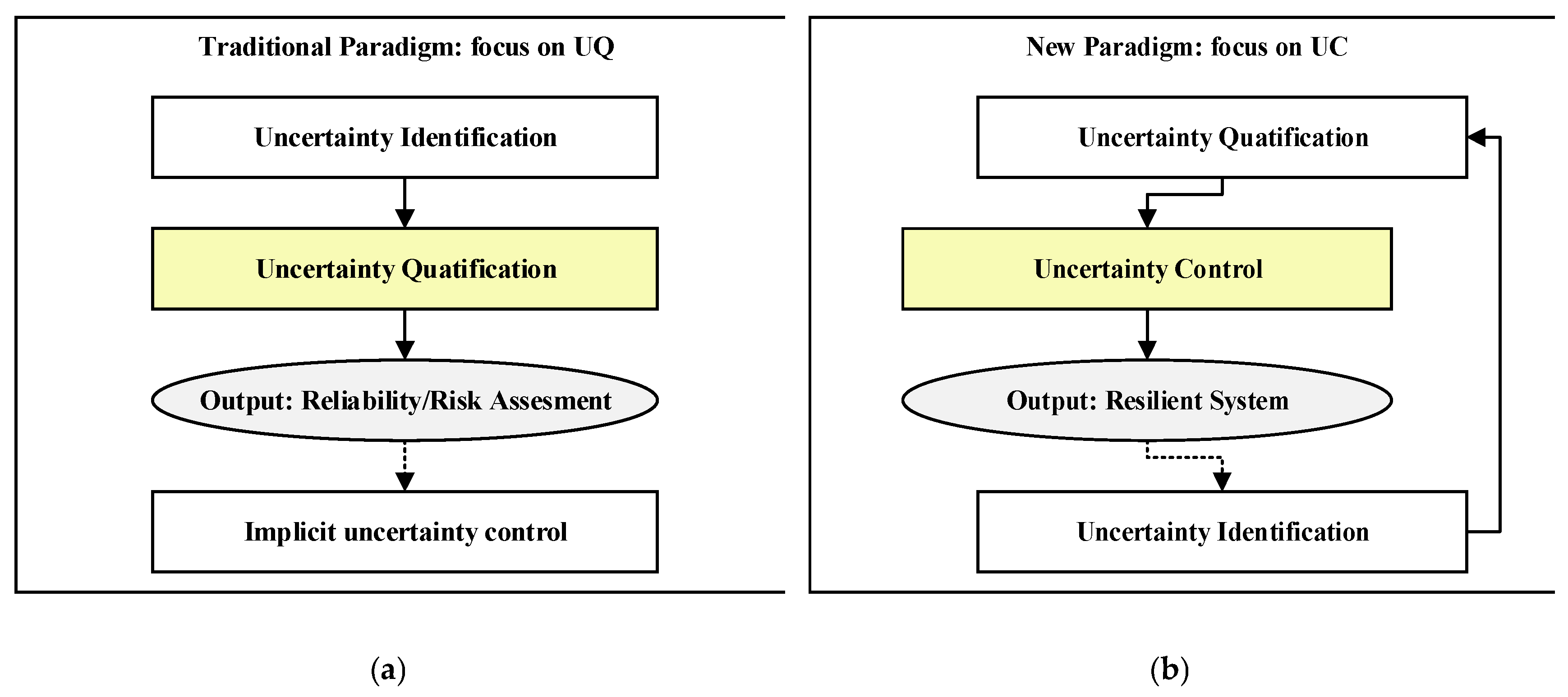
Figure 2.
Illustration for using PoF modeled to obtain reliability of a specific failure mode.
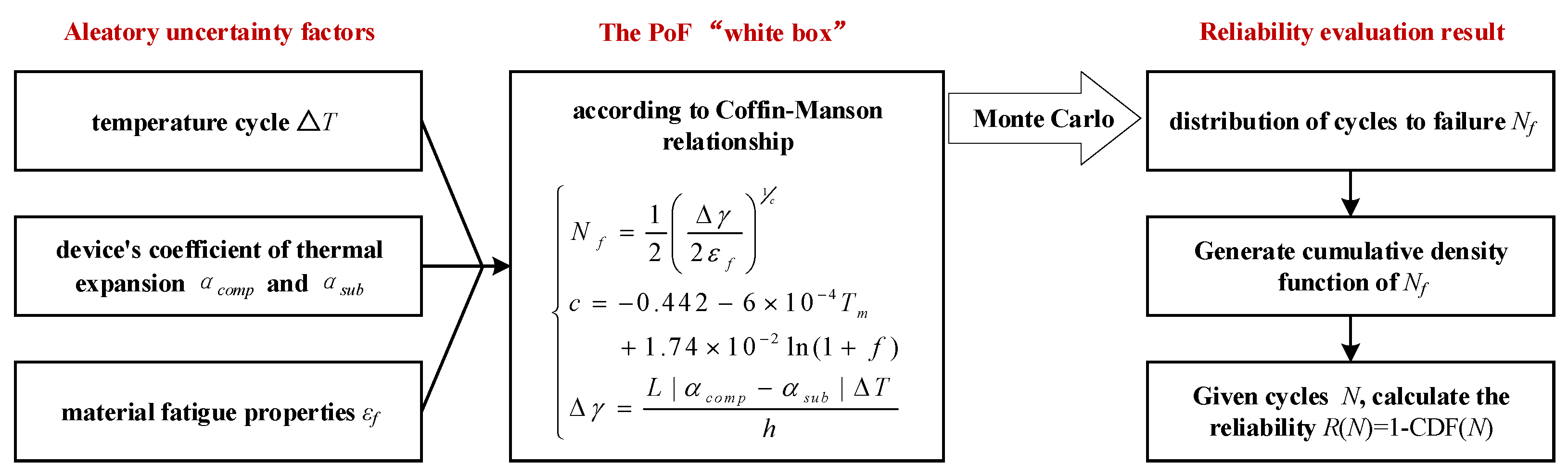
Figure 3.
System RUL evaluation based on the current state of components.
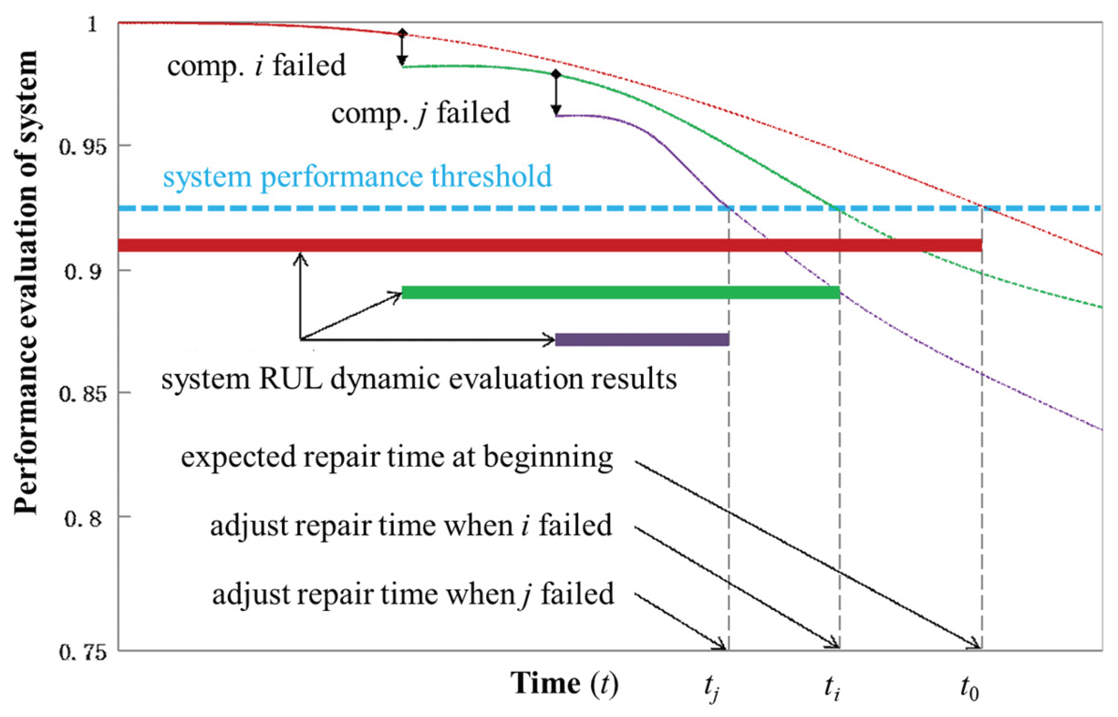
Table 1.
The Comparison of Traditional and Systemic Accident Causality.
| Attribute | Component Failure Model | Systemic AccidentModel |
| Locus of Cause | Physical or software component failure | Unsafe interactions between non-failed components |
| Causal Model | Linear chain of events | Complex feedback loops and systemic structure |
| Safety View | "Safety-I": Safety is the absence of failures | "Safety-II": Safety is an emergent system property |
| Assumption | Reliable components lead to a safe system | A safe system successfully controls its behavior |
Table 2.
The characteristics of reliability paradigm in each era.
| Characteristics |
Statistical Paradigm |
Physic-of-Failure Paradigm |
Prognostic Paradigm |
Resilience Paradigm |
| Developed era | 1950s-1970s | 1980s-1990s | 2000s-2010s | 2020s-present |
| Focus | macro-level failure data | causal failure mechanisms | real-time component health | systemic behavior |
| Goal | quantify population reliability | proactive failure prevention | predict impending failures | mission success under uncertainty |
| Methodology | life data analysis | FMEA/FTA, degradation models | PHM, CBM, HUMS, CMS | RTA, STPA, Resilience Engineering |
| Approach | reactive | preventive | predictive | adaptive |
Table 3.
Other statistical models for reliability and uncertainty analysis.
| Model | Core Principle & Application Value | References |
| Normal dist. | Primarily models aleatory variability in physical parameters (e.g., manufacturing dimensions, material strength, electrical resistance). As a lifetime model, it is limited to pure wear-out phenomena where failures cluster very tightly around a mean with low variance. | [43,44] |
| Lognormal dist. | Models time-to-failure for degradation processes resulting from many small, independent, multiplicative effects. Crucial for modeling wear-out in semiconductor devices, bearing fatigue, and some forms of material corrosion. It is often the primary alternative to the Weibull distribution for wear-out analysis. | [45,46,47] |
| Binomial dist. | Models the number of failures in a fixed number of n trials. It is the statistical foundation for reliability demonstration testing and used to determine the sampling size under acceptable confidence level. | [48,49] |
| Poisson dist. | Models the number of discrete events occurring over a fixed interval of time, area, or volume. Essential for Statistical Process Control (SPC) in manufacturing to monitor and control the rate of non-conformities, such as defects per square meter of a composite layup. | [50,51] |
| Gamma dist. | A flexible distribution that can model waiting times for a series of events. It is a generalization of exponential distribution and is used to model the time to the k-th failure in a repairable system or for systems with standby redundancy. | [52,53,54] |
Table 4.
Key Physics-of-Failure Models for Typical Failure Model in Aerospace Reliability Analysis.
| Failure Mode | Model Purpose & Application | Key Uncertainty Factor | Model Formula | References |
| Mechanical Fatigue |
To predict the number of cycles to failure in metallic structures (e.g., airframe, engine disks) under cyclic stress. Essential for damage-tolerant design and setting inspection intervals. | material constants C, M initial crack size a0 stress intensity factor range ΔK |
Paris's Law | [74,75] |
| Electro- migration |
To predict the Mean-Time-To-Failure (MTTF) of metallic interconnects in integrated circuits due to the "electron wind" effect. Critical for avionics processor and ASIC reliability. | current density J temperature T activation energy Ea material constant A current density exponent n |
Black's Equation | [70,76] |
| Hot Carrier Injection |
To predict transistor lifetime or performance degradation due to high-energy carriers damaging the gate oxide interface. A primary concern for deeply scaled digital logic. | substrate current Isub drain current Id drain voltage Vds technology-dependent constants |
Substrate Current Power Law | [77,78] |
| Negative Bias Temperature Instability |
To model the threshold voltage shift in pMOS transistors, which degrades performance over time. A critical reliability issue in modern avionics and processors. | time t temperature T electric field Eox material/process constants. |
Reaction-Diffusion Model | [79,80] |
| Time- Dependent Dielectric Breakdown |
To predict the time-to-breakdown of the thin gate oxide insulator in a MOSFET. A fundamental lifetime limiter for all modern integrated circuits. | electric field Eox temperature T activation energy Ea field acceleration factor γ |
Thermochemical Model | [81,82] |
Table 5.
The main characteristics of FMEA and FTA.
| Attribute | FMEA | FTA |
| Logic | Bottom-Up: Forward-chaining from cause to effect. | Top-Down: Backward-chaining from effect to cause. |
| Guiding question | What happens if this component fails? | How can this system hazard happen? |
| Purpose | To explore the effects of potential component failures and identify their severity for risk prioritization. | To identify all credible combinations of failures (minimal cut sets) that lead to a specific top-level hazard. |
| Key output | A structured table listing failure modes, their effects, severity, and Risk Priority Number (RPN). | A logical tree diagram, a list of minimal cut sets, and a calculated probability for the top-level event. |
| Core Assumption | System hazards are the result of the summed or sequential effects of individual component failures. | System hazards can be represented as a Boolean combination of basic component-level failure events. |
Disclaimer/Publisher’s Note: The statements, opinions and data contained in all publications are solely those of the individual author(s) and contributor(s) and not of MDPI and/or the editor(s). MDPI and/or the editor(s) disclaim responsibility for any injury to people or property resulting from any ideas, methods, instructions or products referred to in the content. |
© 2025 by the authors. Licensee MDPI, Basel, Switzerland. This article is an open access article distributed under the terms and conditions of the Creative Commons Attribution (CC BY) license (http://creativecommons.org/licenses/by/4.0/).
Copyright: This open access article is published under a Creative Commons CC BY 4.0 license, which permit the free download, distribution, and reuse, provided that the author and preprint are cited in any reuse.


