From the Balkan Peninsula to the Mesic Grassland Areas of Central Europe: Morpho-Genetic Diversity and Niche Differentiation in the Allopolyploid Complex of the Austrian Speedwell

1. Introduction

The Balkan Peninsula has long been acknowledged as a major center of biodiversity [1]. With ca. 6500 species of vascular plants reported, the region is more species-rich than any area of comparable extension within Europe [2]. Among the factors responsible for this amazing species richness are that it is a topographically and climatically diverse region with high geological complexity [3,4], in addition to the fact that it is placed at the junction of three continental regions representing a crossroads of several major floras [5]. The numerous mountain formations display a complex pattern of small blocks geographically close to each other [6] and the large habitat heterogeneity —among those, mesic meadows and other grassland areas, such as prairies and drier steppe-like environments— have led to genetic differentiation among taxa resulting also in a hotspot of endemism [7]. The mainly lowland areas that facilitated the persistence of species during past climatic oscillations may have acted as ‘museums’ for the conservation of diversity, as ‘cradles’ of new diversity (i.e., regional biodiversity hotspots; [8,9]) and may have also provided corridors allowing migrations of plant species from grassland habitats.

Despite its species-richness, its importance as a centre of diversification, and its role as a major source of postglacial colonization of Central and Northern Europe, not much is known about the patterns of diversity and phylogeography of biota from the Balkans, as compared to the Italian and Iberian peninsulas. Many groups of organisms remain unstudied [10] and detailed studies centered in the Balkan Peninsula have mostly put their focal point on vertebrates (and specially herpetofauna; e.g., [11,12]), butterflies (e.g., [13]) or alpine plants (e.g., [14,15]). In contrast, only a few studies (e.g., [16]) have been focused on nowadays widely distributed plant species representative of dry to mesic grassland habitats from Europe. These environments, which are potentially common in Eurasia have been traditionally subjected to high pressure mainly from agriculture and forestry and suffer many times from severe fragmentation. Therefore, additional studies are necessary to better achieve their conservation.

Among the different mechanisms involved in diversification, polyploidization has played a major role in the evolution of many taxa within the Balkan Peninsula (e.g., [17,18]). Polyploidization has been proposed to have facilitated the colonization of new niches available after the climatic oscillations of the Quaternary and would therefore be involved in the post-glacial expansion of some species (or cytogenetic units) during the Holocene [19,20]. Particularly, allopolyploidy has been proposed as a major mode of speciation (e.g., [21]) and is believed to favour both niche (e.g., [22]) and, at least in particular cases [23,24], range expansion (but see [25]). Several studies utilizing novel methods −among them, Species Distribution Models (SDMs)− (e.g., [26]) have indicated that the ecological niches of allopolyploids often differ from at least one of their lower ploidy ancestors (e.g., [27]). In contrast, other investigations suggest that allopolyploids may occupy intermediate or non-divergent ecological niches (e.g., [28]). Consequently, additional studies are necessary to interpret which is the role that niche shift plays in the establishment of polyploid lineages.

Species are often used as the basic units of analysis in biogeography. However, species can be described as an assemblage of genetic lineages varying in their genetic inter-relationship and spatial distribution [29]. Thus, addressing intraspecific genetic variation of widely distributed species within an ecogeographic context is necessary to understand key topics in ecology, evolution and biogeography [30] and can even provide valuable information for conservation [31]. The value of intraspecific genetic variation has recently increased its relevance mostly due to the implications for forecasting the response of distinct genetic units under climate change [29]. Facing a context of biodiversity loss, it is necessary to highlight that intraspecific genetic variation is the most fundamental level of biodiversity, provides the basis for any evolutionary change and is crucial for maintaining the ability of species to adapt to environmental conditions [32,33]. Widespread species from common environments provide opportunities to study both genetic and phenotypic variation patterns across ample ranges of climatic conditions. Large-scale studies are needed to identify candidate adaptive traits and their relationships with their putative selective environmental agents. Determining these patterns becomes a crucial preliminary step to design studies specifically aimed to understand the genomic basis underlying local adaptation in climate-related traits [34].

Here, the geographically widespread allopolyploid complex of the Austrian speedwell (hereafter, V. austriaca complex) was selected to investigate whether the combination of subgenomes in an allopolyploid species may yield plants with increased genetic and morphological diversity, as well as enhanced colonization abilities. The V. austriaca complex is composed of suffrutex perennial herbs that occur in vast regions from Central and Eastern Europe and Asia. Taxonomically, it belongs to Veronica subsect. Pentasepalae Benth., and comprises the diploid V. dalmatica Padilla-García, Rojas-Andrés, López-González & M.M.Mart.Ort., an uncertain tetraploid entity and the hexaploid V. austriaca L.

In this study, the species name V. austriaca L. is applied according to the last available taxonomic treatment [35], with the modifications introduced by the results derived from Padilla-García et al. [36] and López-González et al. [37], which means that V. austriaca includes only hexaploids. While many narrow endemics can be found within Veronica subsect. Pentasepalae [36], only a few species —among them V. austriaca— are widely distributed. Furthermore, V. austriaca displays wide ecological amplitude and is therefore present in a variety of habitats, being mostly represented in grassland areas (from mesic meadows to Mediterranean dry steppe-like environments) and sometimes in grassy forest glades or forest edges. It extends also to a wide array of climatic and altitudinal (60-2000 m) conditions all throughout the Balkan Peninsula, Central Europe, and —according to Borissova [38]— it is also present in Belarus, European Russia, Moldavia, Ukraine and S Caucasus.

In addition to the wide ecological preferences, V. austriaca displays high morphological diversity. Thus, several infraspecific taxa [usually three subspecies, i.e., V. austriaca subsp. austriaca, V. austriaca subsp. dentata (F.W. Schmidt) Watzl and V. austriaca subsp. jacquinii (Baumg.) Watzl] have been described within the variation of this taxonomically challenging species. There is for example a gradient regarding leaf incision that has been interpreted by different authors in different ways, with the description of the individuals that show intermediate character states either as “transitional forms” between subspecies or as taxonomic entities of hybrid origin [39,40]. Recently, it has turned out that some of these populations from the Western Balkans that show intermediate character states are the result of allopolyploid events [36]. Specifically, in the formation of the hexaploid V. austriaca (subsp. jacquinii), the diploid species Veronica dalmatica and a scientifically still unnamed “uncertain tetraploid” have been involved, with the possibility of recent gene flow among these different cytotypes [37]. Thus, both taxonomic entities (i.e., 2x and 4x lineages), together with the hexaploid V. austriaca, conform the V. austriaca allopolyploid complex, which is the object of this study.

Thus, we here investigate the diversity patterns of this allopolyploid complex across its range in the Balkan Peninsula and Central Europe. For this, a combined approach is applied using ploidy levels estimated by flow cytometry (FCM), data from nuclear markers (Simple Sequence Repeats, SSRs) and plastid DNA (cpDNA) sequences. Phenotypic and ecological variation are also considered, respectively, through the morphometric analysis of several leaf and fruit characters, through the prediction of the ecological niche optimum and breadth of the members of the allopolyploid complex, as well as the prediction of the present potential distribution areas of the hexaploid V. austriaca using SDMs. The specific goals are: (1) to assess the genetic structure and diversity in V. austriaca and its putative diploid and tetraploid ancestors; (2) to describe the morphological variability and ecological niche breadth of the members of the allopolyploid complex; (3) to understand the historical processes that may have been responsible for the contemporary geographic distribution of the populations of the hexaploid V. austriaca and, (4) to evaluate the impact that allopolyploidy may have had in the colonization abilities and expansion of a species that is nowadays widely distributed in the mesic grassland areas of Europe.

2. Materials and Methods

2.1. Plant Material

Details about location and taxonomic assignment of the samples included are provided in Table S1. The spatial distribution of the selected populations is displayed in Figure 1. Fresh leaf material was collected and stored in silica gel. The complete dataset comprises 751 individuals corresponding to 50 populations. A mean of 15 (from 4-20) individuals per population were sampled whenever possible, given that many times populations were very small. Initial plant identification was based on the most recent taxonomic treatment by Rojas-Andrés and Martínez-Ortega [35] with modifications from Padilla-García et al. [36] and López-González et al. [37]. Vouchers were deposited in the herbarium SALA (abbreviation according to Thiers [41], continuously updated).

2.2. DNA Ploidy Level Estimations

DNA-ploidy levels were estimated by flow cytometry (FCM) from silica gel dried leaves. For the present study, measurements on 456 individuals were newly generated; the remaining estimations were obtained from López-González et al. [37]. Nuclear suspensions were prepared following the method described by Galbraith et al. [42]. Leaf tissue of either one individual or two to six individuals was chopped together with leaf tissue from an internal standard using a sharp razor blade in a Petri dish with Woody Plant Buffer solution with slight modifications [43]. Several internal standards were employed depending on the C-value and standard availability: Raphanus sativus L. (2C = 1.11 pg; [44]), Solanum lycopersicum L. (2C= 1.96 pg; [44]), Solanum pseudocapsicum L. (2C = 2.59 pg; [45]), Zea mays L. cv. ‘CE-777’ (2C = 5.43; [46]), Pisum sativum L. cv. ‘Kleine Rheinländerin’ (2C = 8.84; [47]), and Pisum sativum L. cv. ‘Ctirad’ (2C = 9.09; [49]). Nuclear suspensions were filtered through a 48 μm nylon mesh, incubated with RNase and stained with a saturating solution of propidium iodide (PI) following Loureiro et al. [43] and Rojas-Andrés et al. [49].

For each individual, one run of 5000 counts was made on a CyFlow Space (Partec GmbH, Münster, Germany; equipped with a 532 nm solid-state laser). Results were acquired through the Partec FloMax software v2.4d (Partec GmbH, Münster, Germany). DNA-ploidy level was estimated for each sample based on the C-values and the available chromosome counts for the studied species [50,51].

2.3. Laboratory Procedures

2.3.1. DNA Extraction

Total genomic DNA was extracted from silica-gel-dried material following the CTAB protocol [52] with slight modifications. For each individual, 20-25 mg of dried leaves were used. The quality of the extracted DNA was checked on 1% TAE-agarose gels and the amount of DNA was estimated using a Nanodrop 2000C Spectrophotometer (Thermo Scientific). DNA extractions are deposited at the Biobanco de ADN Vegetal of the University of Salamanca (Spain).

2.3.2. SSR Amplification, Fragment Analysis and Genotyping

Twelve SSR polymorphic primer pairs were employed (see Table 1 in López-González et al. [53]) to genotype the 751 individuals corresponding to the whole dataset. Following the procedure developed by Schuelke [54], the sequence-specific forward primers were marked at the 5′ end with an M13 tail (5′-TGTAAAACGACGGCCAGT-3′) (Eurofins) and then labeled with 5-FAM, VIC, NED, or PET fluorescent dyes (see Table 1 in [53]) (Life Technologies). PCR conditions were as follows: an initial step at 94°C for 2 min; followed by 35 cycles of 1 min at 94°C, 1 min at 50–58°C, and 50 s at 72°C; 10 cycles of 1 min at 94°C, 1 min at 53°C, and 50 s at 72°C and a final extension of 15 min at 72°C. Reaction volumes (total volume: 15 μL) included: 50 ng of DNA template, 5 μL 5×Green GoTaq Reaction Buffer (Promega), 0.2 mM of each dNTP, 0.16 mM of each reverse and fluorescent-labeled M13 primer, 0.04 mM of forward primer and 0.75 units GoTaq DNA Polymerase (Promega). All PCR reactions were performed on a Mastercycler-Pro thermocycler (Eppendorf). PCR products were visualized on 2.5% TBE-agarose gels and multiplexed for genotyping. Fragment analysis was conducted at the Unidad de Genómica-Campus Moncloa (Universidad Complutense de Madrid, Madrid, Spain) using the internal GeneScan 500 LIZ Size Standard (Applied Biosystems) in a multi-capillary sequencer ABI Prism 3730 (Applied Biosystems). Genotyping was performed through GeneMarker Software version 1.8 (SoftGenetics, State College, Pennsylvania, USA) and the peaks were scored manually.

Reproducibility tests were performed over 5-10% of the total number of individuals. Two to three independent runs at different times were carried out. The outcomes indicated 95% match in the results, suggesting that the microsatellite analyses are highly reproducible.

2.3.3. Plastid DNA Amplification and Sequencing

The plastid DNA regions trnH-psbA and ycf6-psbM were amplified for 312 selected individuals from the total dataset (4 to 13 individuals per population). From these, 176 sequences of each region were newly generated, while the remaining ones were obtained from Rojas-Andrés et al. [49] or from López-González et al. [37]. These plastid regions were chosen following Rojas-Andrés et al. [49] due to their high levels of variability. The ycf6-psbM spacer was amplified using the ycf6F forward and psbMR reverse primers [55], and the trnH-psbA spacer with the forward primer psbA [56] and the reverse primer trnH2 [57]. PCR conditions for the amplification consisted of an initial denaturation cycle of 2 min at 95 °C followed by 40 denaturation cycles of 30 s at 95 °C, annealing for 30 s at 55 °C, and extension for 2 min 30 s at 72 °C, followed by a final extension phase of 10 min at 72 °C. The reaction volumes (total volume: 25 μL) included: 36 ng of DNA template, 5 μL 5×Green GoTaq Reaction Buffer (Promega), 0.2 mm dNTPs, 0.3 μm each primer and 0.85 units GoTaq DNA Polymerase (Promega). All PCR reactions were performed on an Eppendorf-Mastercycler-Pro thermocycler. All amplified fragments were visualized on 1% TBE-agarose gels and purified with ExoSap-IT (USB Corporation) following the manufacturer's instructions. PCR products were sequenced by Macrogen Inc. (Seoul, Korea) using an ABI Prism 3730XL DNA analyser (Applied Biosystems). Accession numbers of the sequences obtained from Rojas-Andrés et al. [49] are KT361722 - KT361723, KT361726 - KT361728, KT361731 - KT361733 and KT361775, KT361778 - KT361780, KT361783 - KT361785 (trnH-psbA and ycf6-psbM respectively). Accession numbers of the sequences obtained from López-González et al. [37] are MN997128 - MN997307 (trnH-psbA) and MT084169 - MT084346 (ycf6-psbM). The newly generated sequence data have been deposited in the European Nucleotide Archive (ENA) at EMBL-EBI under the project accession number PRJEB102049 (OZ360793 – OZ360968) (trnH-psbA) and PRJEB102053 (OZ360969 – OZ361144) (ycf6-psbM).

2.4. DNA Data Analyses

Given that genotyping of SSRs with hexaploids shows a remarkable drawback, due to the difficulty of distinguishing the exact number of copies for a given allele [58], the scoring was done indicating the alleles that were present in each individual and the rest of the copies were coded as missing data. The summary statistics were calculated using the original matrix (individuals × allele length) with SPAGeDi [59]. Given that this software detected a high proportion of incomplete genotypes in the dataset, which may prevent an accurate assessment of genetic diversity, a presence/absence matrix was generated to calculate this parameter with AFLPdiv 1.1 [60] and Popgene v. 1.32 [61], and compare general patterns. Spatial distribution of genetic diversity was represented using ‘sf’, ‘rnaturalearth’, ‘rnaturalearthdata’ and ‘ggplot2’ packages in R [62,63,64,65] and the diversity boxplots were represented using ‘ggplot2’ and ‘tidyr’ packages in R [65,66].

To infer population structure and assign individuals to populations based on the SSR genotypes a Bayesian clustering analysis based on the MCMC algorithm was performed using Structure v.2.3.4 [67] with the original matrix as an input. Multiple runs of Structure were performed by setting K from one to ten. The burn-in time and replication number was set to 1×10⁶ for each run and 10 runs were done for each value of K. To determine the most probable value of K, StructureSelector [68] was used following the criterion described by Evanno et al. [69]. Results of independent Structure runs were summarized and visualized using both StructureSelector and CLUMPAK (Cluster Markov Packager Across K) [70]. A map with bar-plots displaying the probability of belonging to a cluster (by population) was elaborated using the software ArcMap v. 10.6 [71].

Additionally, given that it was our aim to explore the expansion of the hexaploid V. austriaca and in order to visualize differentiation among possible genetic groups within this ploidy level, a Discriminant Analysis of Principal Components (DAPC; [72]) was completed using the ‘adegenet’ package in R [73] with no a priori assignment of individuals to groups and using the presence/absence matrix (excluding monomorphic alleles in the hexaploids) as an input. A minimum-spanning tree connecting the cluster centroids based on the squared distances among populations was superimposed.

Regarding the plastid DNA sequence data, the alignment was carried out using SATé [74] and visualized in Geneious Pro v. 6.0.6. (Biomatters). Gaps and non-informative variable sites were removed with Gblocks0.91b [75], keeping the default parameters. Inversions were found in the analysed regions and were subsequently removed from the sequences. Mononucleotide repeats of different sizes were excluded because they seem to be prone to homoplasy at large geographical scales [76]. Plastid DNA sequences were used to construct an unrooted haplotype network. The statistical parsimony algorithm [77] was applied to infer the genealogical relationships among haplotypes through the TCS 1.21 software [78]. The ambiguities encountered in the haplotype network, which are probably due to homoplasy (recurrent mutations) and/or recombination within DNA regions [79], were resolved by following the guidelines in Crandall & Templeton [80], based on the frequency of appearance of the different alleles and the geographic location of the samples involved.

2.5. Morphometrics

Five fruit characters and twenty leaf characters (abbreviations shown in Table S2) were measured for all 50 populations included in this study. Fruit characters were measured in three specimens per population, and five fruits per specimen were considered. Leaf characters were measured in three specimens per population except for cases in which the available material was insufficient. Leaf measurements were taken from two different leaves: one situated in the central segment of the stem (medium leaf) (see Figure 2 in Andrés-Sánchez et al. [81] for further details) and another one on the apical shoot (see Figure 3 in [81]).

Leaf measurements, except those related to the indumentum, were taken with a digital electronic caliper Digimatic 500 (Mitutoyo American Corporation, Aurora, USA). One measurement was made for each variable except for hair length, for which five trichomes per leaf were considered. Hair “density” was indirectly estimated by counting the number of hairs on 1 cm-long linear transects at the leaf margin and at the medium part of the leaf. Hair length, “density” and fruit measurements were determined by means of a stereoscopic zoom microscope NIKON SMZ-U (Nikon Corporation, Tokyo, Japan) equipped with a video camera SONY 3CCD DXC-930P (Sony Corporation, Tokyo Japan). The photos taken were transferred to a computer and examined through the image-analysis software Image-Pro Plus version 1.0 (Media Cybernetics Inc., Rockville, USA). In an effort to avoid the size effect, some characters were considered as quotients. Arithmetic means were calculated and variables were assessed individually in a visual exploration through boxplots considering different groupings in order to explore differences: among ploidy levels; among the genetic-geographic groups obtained through the Bayesian analysis and DAPC of SSRs data (see Results) within the hexaploid species V. austriaca and between the cryptic taxa V. dalmatica and V. austriaca ssp. jacquinii. ANOVA tests were also performed to check for statistically significant differences. The boxplots and their corresponding ANOVA tests were calculated using ‘ggplot2’ and ‘car’ packages in R [65,82].

2.6. Analyses Based on Climatic Variables

The localities used for these analyses were only those visited by the authors, where the presence of the relevant taxonomic entity was confirmed. Geographical coordinates were collected during fieldwork using GPS.

2.6.1. Species Distribution Models (SDMs)

SDMs were performed to investigate present niche availability for the three genetic-geographic groups detected by SSRs within the hexaploid V. austriaca. Values were extracted from the layers in the V. austriaca occurrences with the function ‘extract’ of the R package ‘raster’ [83]. Spatial resolution was 2.5 arc-minutes for all of them. The layers were trimmed around the occurrences of V. austriaca in the study area (extent: 10° N, 35° W to 30° N, 50° W) using ‘raster’ [83]. Each layer was converted to BIL format. The columns (i.e., environmental variables) of this primary matrix were checked for high (>|0.80|) pairwise correlation. Variables lacking high correlation values were retained. The layers were separated into groups according to correlation values to be able to sequentially select one of each group in further steps. For the GLMs, occurrences were classified according to the molecular groups obtained by Bayesian clustering and DAPC. Background points were generated through the formula ‘randomPoints’ included in the ‘dismo’ R package [84]. The background points were generated across the entire range to provide a comparative data set to be contrasted against the occurrences. The final set of variables for each molecular group was selected after applying the variance inflation factor values (VIF; [85]) over the models. These analyses were performed through the ‘vif’ function of the ‘HH’ package [86] to test for absence of multicollinearity.

Once the set of variables was determined for each hexaploid genetic-geographic group, final models were performed combining GLMs with three frequently used modelling techniques: random forest (RF; [87]), artificial neural networks (ANNs; [88]), and maximum entropy (ME; [89]). Recent studies have suggested that machine-learning methodology may perform better than the traditional regression-based algorithms [90]. RF, ANNs and ME are considered to be among the most powerful machine learning algorithms for ecological prediction [91,92,93] and for obtaining powerful ensemble models [94,95]. Predictions from single SDMs are commonly highly variable and unreliable while ensemble approaches could yield more accurate predictions [96].

Modelling with RF, ANN and GLM was performed using the R package ‘Biomod2’ [97] and for the ME algorithm the ‘ENMeval’ library was employed [98]. RF, ANN and GLM models were carried out using a randomly chosen 75% of the data with the remaining 25% used for cross-validation to assess the performance of each model using the area under the receiver operator curve (AUC-ROC) assessment criteria. Five replicates were run for each model. Contribution of each variable was calculated as a weighted average of the AUC-ROC values obtained in the selected models. It was calculated separately for the different algorithms.

The ME models were run with the feature classes L, Q, H, LQ and LQH (where L = linear, Q = quadratic, H = hinge), and a regularization multiplier (rm) from 0.5 to 2 by 0.5 steps. The selected method was also k-fold strategy with five replicates. The area under the curve (AUC) and the AIC corrected for small sample sizes (AICc) were used to evaluate the models. Following these criteria, the model showing the lowest AICc was selected if the AUC value was above 0.8 [99]. For each hexaploid genetic-geographic group, the best-performing RF, ANN and GLM models (AUC-ROC > 0.95) and the best model resulting among ME models were selected to build an ensemble forecasting species distribution model. The ensemble forecasts are calculated as the mean of the individual model predictions weighted by AUC-ROC scores. To identify areas of probable ecological contact between pairs of hexaploid genetic-geographic groups, models were transformed to presence/absence. For this, cells with values over 0.5 were considered for presenting suitable habitats for the species.

This procedure is parallel to that followed by López-González et al. [37], where projections corresponding to distribution models onto the climatic scenarios of the present climatic conditions, as well as for those of the Mid-Holocene (6 ka BP) and Last Glacial Maximum (22 ka BP) were already published for the diploid species V. dalmatica in the study area.

2.6.2. Niche Comparison Analyses

The 19 environmental layers of the BioClim dataset from the WorldClim database at 30-s (c. 1 km) resolution (Worldclim Version2; [100]), together with altitude information [101] were initially considered. Climatic niche comparisons were performed between pairs of ploidy levels (2x vs. 4x, 2x vs. 6x and 4x vs. 6x) given that it was our aim to explore niche differentiation among hexaploids and their putative ancestors. For niche quantification, it is recommended to filter records to avoid unequal representation of samples caused by sampling bias, which potentially would give rise to the assumption of independence among occurrence data [102]. Following this recommendation a minimum distance filter was applied to prevent points closer than 10-km distance within each entity. All original records satisfied this criterion; thus, 50 presence records were considered for the analyses: 9 for the diploids, 9 for the tetraploids and 32 for the hexaploids. To elucidate the autocorrelation of variables, we calculated Pearson correlations. Within each set of variables showing a correlation < 0.7, we selected those showing the lowest values of VIF. Eight bioclimatic variables were finally selected. For the niche comparison analysis, we applied the method developed by Broennimann et al. [103]. Niche overlap between hexaploids and its putative ancestors was calculated using the R package ‘ecospat’ [104]. This calculation is based on Schoener's D metric [105] that ranges from 0 (no overlap) to 1 (complete overlap). The procedure and metrics are described in detail in Padilla-García et al. [106]. Niche breadth was also calculated following the procedure described in Theodoridis et al. [107], Kirchheimer et al. [108] and Padilla-García et al. [106]. The results were visualized using boxplots for each PCA axis and ANOVA test were performed to test for the significant differences on the niche breadth among the studied diploid and polyploid entities.

3. Results

3.1. DNA Ploidy Level Estimations

Ploidy levels were newly estimated for 456 individuals according to the 1C-values obtained. Ninety-one per cent of the measurements presented a sample coefficient of variation (CV) of G1 peaks below 5%, while the CV of the remaining measurements was between 5 and 7.9 %. All values were accepted for ploidy level estimation. Considering only measurements with CVs < 5% genome size values ranged from 1.11 to 2.13 pg. The variation was not continuous and the 1C-values were arranged in two groups corresponding to two different ploidy levels: 4x (populations 39, 45 and 47; Figure 1; Table S3) and 6x (remaining populations; see Figure 1; Table 1 and Table S3). Genome size values corresponding to the diploid level were not found. Nuclear DNA contents ranged between 1.11 and 1.32 pg for tetraploids and between 1.67 and 2.13 pg for hexaploids (Table S3). All populations were composed of a single cytotype.

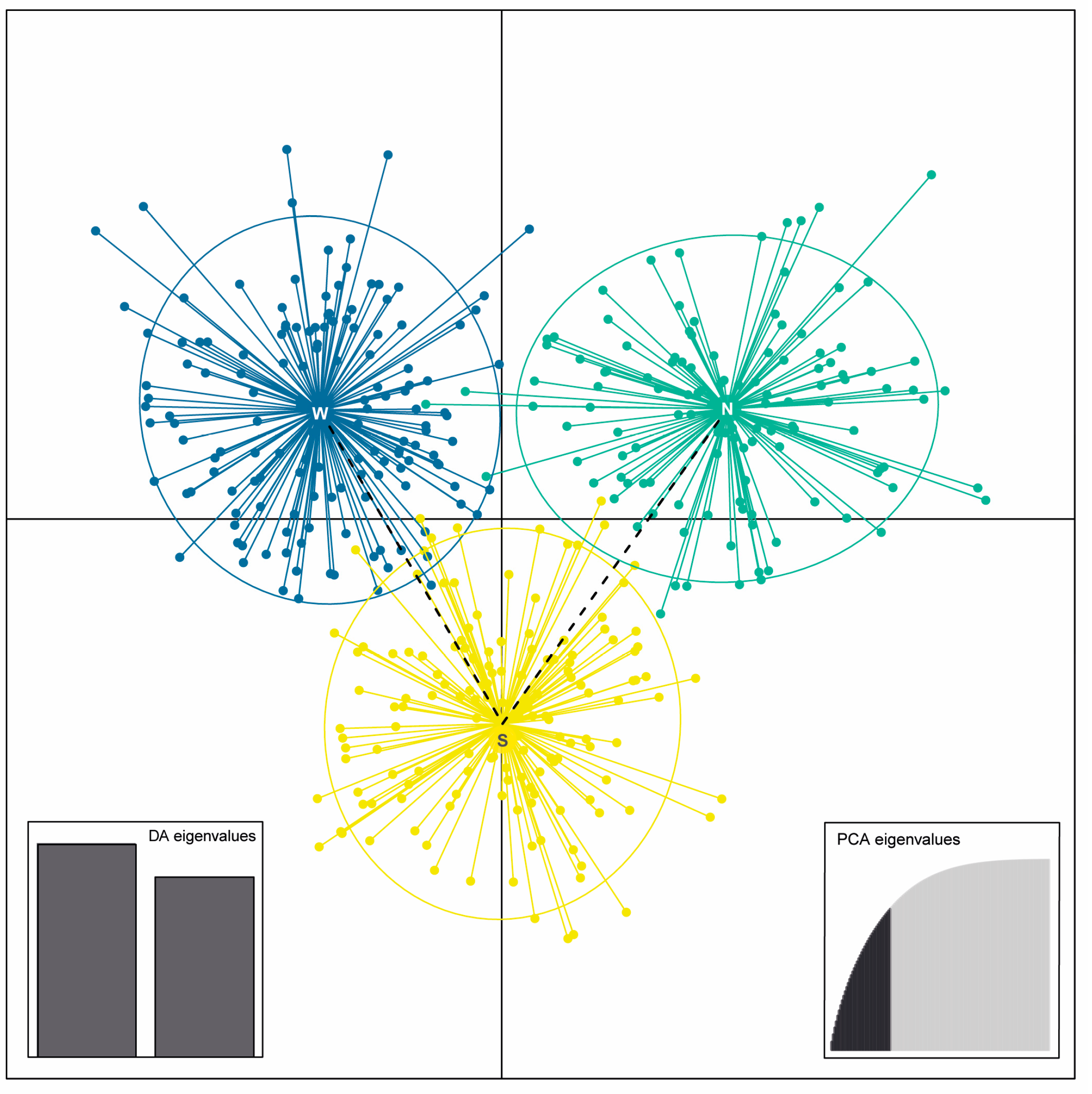
3.2. Genetic Structure and Population Differentiation Based on SSR Markers

From the initial set of microsatellites, two were deprecated due to genotyping incongruence and presence of indels. A total of 156 alleles were amplified from the 10 microsatellite loci that provided reliable genotypes. The SPAGeDi software applied to the original matrix reported 88.4% missing data globally (across all individuals and loci). As this situation may affect the accuracy of interpreting genetic diversity estimates and considering that results derived from the matrix that includes allele length information also detected parallel diversity patterns, only the results derived from the latter approach are commented here (results derived from the presence/absence matrix are available from the authors upon request). Table 1 shows the genetic diversity coefficient h (Nei's genetic diversity index), as the most biologically meaningful summary statistic. The comparison of genetic diversity among ploidy levels (Figure 2a) and the spatial distribution of genetic diversity across the study area (Figure 2b) show that genetic diversity values are maximum in the hexaploid populations and minimum in the diploid ones.

According to the method proposed by Evanno et al. [69] the best value for K is 2, with the next best values at K = 3 and K = 5 (Figure S1). Although the real K is probably K = 2, higher values of K are justified especially if population assignments make biological sense [109] and individuals are strongly assigned to all clusters [110]. Results derived from the Bayesian clustering analyses for K values from 1 to 7 are presented in Figure S2.

The grouping found considering K = 5 is overall consistent with results obtained from DAPC (Figure S3) and with the haplotype network (see below) and makes both most biological and geographic sense. This grouping option results in the following clusters (i.e., SSR lineages; Figure 3): one represented in the southern area (North Macedonia, Bulgaria, and Greece) that is conformed only by hexaploids (cluster 1, yellow); a second lineage composed of diploids restricted to the southeast of the Neretva river (cluster 2, aquamarine); a third cluster, which is made of the hexaploids extended to the north-western part of the study area (cluster 3, dark blue); cluster 4 (violet) that is formed by the tetraploids from the central-western part of the region; and a fifth cluster (cluster 5, emerald green) mainly represented to the north (Austria, Hungary, Slovakia, and Romania), which is mostly composed of hexaploids, plus three geographically close tetraploid populations (pops. 39, 45 and 47).

For convenience, considering that clusters 2 (diploids) and 4 (tetraploids) result mainly from differences in ploidy levels with respect to the remaining ones, the DAPC with no a priori assignment of individuals to groups shown here (Figure 4) includes only hexaploid individuals. Three distinct genetic groups were found that fully correspond with the three genetic clusters that mostly contain hexaploids identified through the just described Bayesian analyses (i.e., clusters 1, 3 and 5). The superimposed minimum spanning tree shows that the northern and western genetic groups are connected through the southern one.

Therefore, in order to facilitate discussion of results, three main genetic-geographic groups will be discussed onwards within the hexaploid species V. austriaca: (i) the southern group (cluster 1); (ii) the western group (cluster 3); and (iii) the northern group (cluster 5).

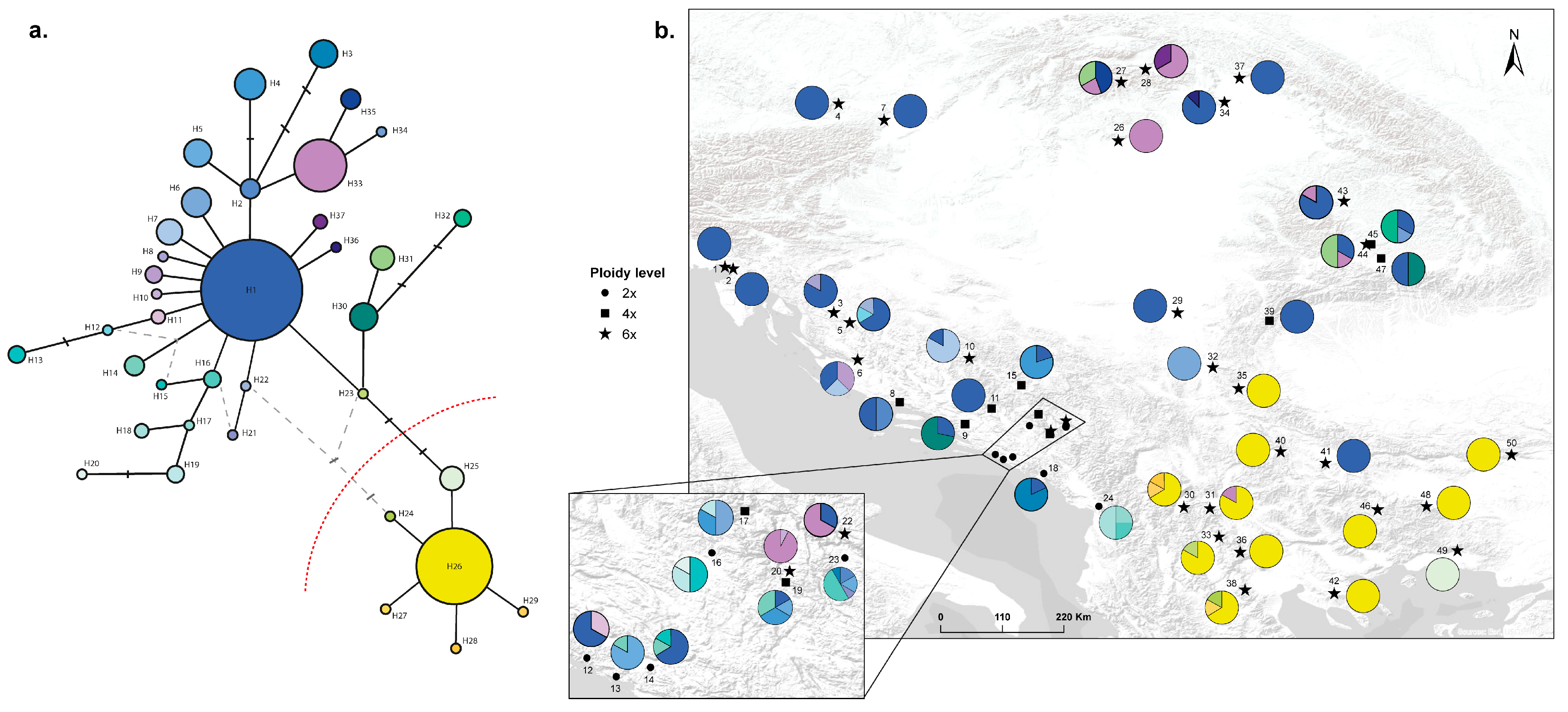
3.3. Analysis of the Plastid DNA Sequence Data

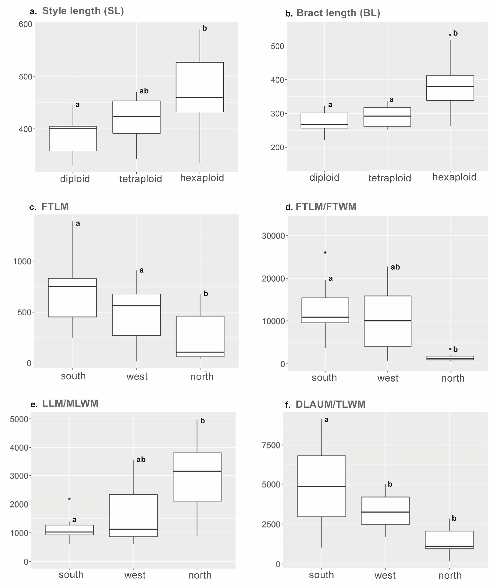
The total length of the 298 cpDNA sequences was 261-272 bp and 581-588 bp for the trnH-psbA and ycf6-psbM plastid regions, respectively. The two regions showed 13 (trnH-psbA) and 11 (ycf6-psbM) polymorphic sites, which led to a total of 37 haplotypes.

Overall, the resulting haplotype network was complex (Figure 5a), but two clear main haplogroups were found that are geographically well structured (Table 1; Figure 5b): a southern haplogroup, which corresponds with the southern genetic-geographic group and a northern haplogroup that included the remaining samples included in this study. Within the northern haplogroup H1 was dominant, while H26 predominated within the southern haplogroup (Figure 5a) and both predominant haplotypes were connected by five parsimony mutation steps.

3.4. Morphometrics

Morphometric measurements comprised a total of 60 fruit and leaf characters including those that were considered as quotients to avoid size effect. Style and bract length, both measured in fruitful individuals (SL and BL) were the most helpful characters to distinguish individuals according to their ploidy level (Figure 6a and Figure 6b). SL was significantly different between diploids and hexaploids and BL discriminated significantly not only between that ploidy pair, but also between hexaploids and tetraploids (Table 2).

Regarding specific differences between the cryptic V. dalmatica and V. austriaca ssp. jacquinii, the main morphometric characters used in the diagnosis of the first given by Padilla-García et al. [36] were revisited. Style and bract length (SL and BL) were identified as the best diagnostic traits to distinguish between these two taxa (Figure S4; Table 3).

When considering the three genetic-geographic groups obtained within the hexaploid V. austriaca, the most discriminant characters were related to leaf shape, which is in accordance with the traditional organization of the morphological variability of V. austriaca into three morphological groups or subspecies based on foliar traits. The most obvious differences appeared between the [southern genetic-geographic group + western one] versus [northern genetic-geographic group]. Thus, although the length of the first tooth of the mid-stem leaf (FTLM) showed slightly overlapping values between these two groups (Figure 6c), the differences were found to be significant (Table 4). The value of the ratio of the length to the width of the first tooth of the mid-stem leaf (FTLM/FTWM) was clearly higher in the southern genetic-geographic group as compared to the northern one (Figure 6d; Table 4), which indicates that the leaves of the mid-stem of the individuals from the southern genetic-geographic group are more divided. As for the individuals of the northern group, they have wider leaves compared to the other lineages, suggesting that the ratio of total length to maximum width of the mid-stem leaf (LLM/MLWM; Figure 6e; Table 4) could be used to distinguish between these genetic-geographic groups. Additionally, both the ratio maximum length-to-maximum width of the mid-stem leaf (LLM/MLWM) and the ratio between the distance from the apex to the first tooth and the width of the entire terminal portion of this leaf (DLAUM/TLWM; Figure 6f; Table 4) indicated a general tendency (more than a clearly significant differentiation in absolute values) to a morphological separation among the three groups.

3.5. Analyses Based on Environmental Variables

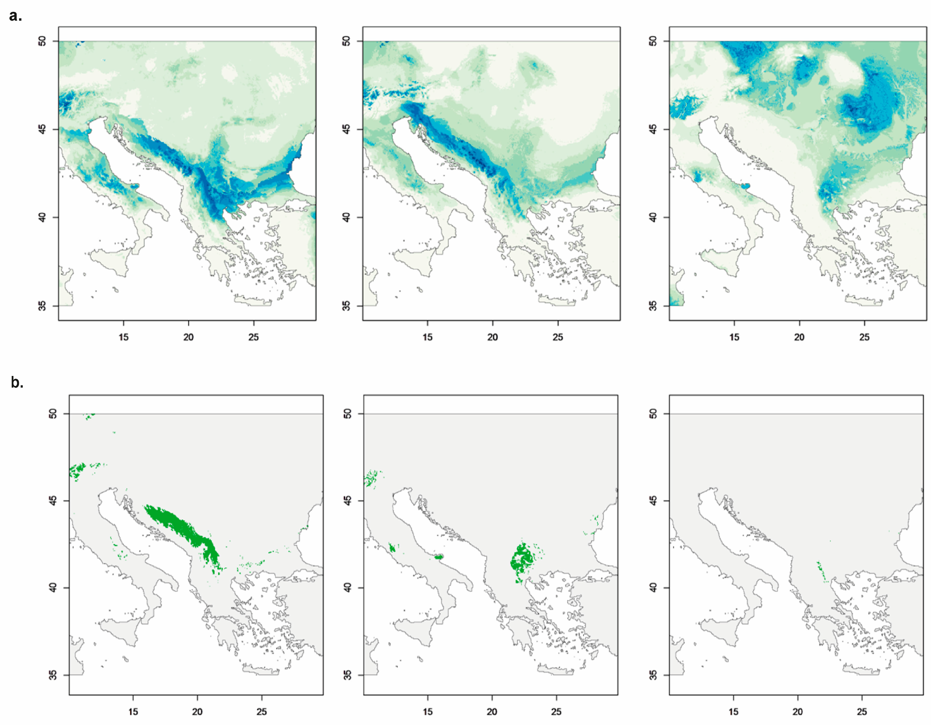
3.5.1. Species Distribution Models for the Three Genetic-Geographic Groups Found Within V. austriaca

The following variables were finally selected: BIO8 (mean temperature of wettest quarter), BIO15 (precipitation seasonality), and BIO19 (precipitation of the coldest quarter) for the southern genetic-geographic group; BIO12 (annual precipitation), BIO15, and BIO18 (precipitation of warmest quarter) for the western genetic-geographic group; BIO19 and altitude for the northern one. From these, BIO8, BIO15 and BIO19 were the most important variables corresponding to the southern, western and northern groups respectively. Variable contribution for each modelling approach is shown in Table 5. Although with different values, the variables with the highest contribution for each genetic-geographic group were the same regardless of the algorithm employed.

A total of 14 models were selected for the southern group, 15 for the western one and 9 for the northern lineage. No GLMs with AUC-ROC scores over 0.95 were found in the last case. The ME models selected were: L for the first group with a regularization multiplier of 0.5; LQ for the second with the same regularization multiplier; and LQH with a regularization multiplier of 2 for the northern genetic-geographic group. These models were those showing the lowest AICc given that the lowest value of AUC was above the threshold established (0.85 for the northern lineage). Final ensemble forecasting models for each genetic-geographic group are shown in Figure 7a. The potential distribution of the southern lineage appears in the area south of the Danube throughout a wide range of altitudes, including the central and southern parts of the Dinaric Alps. The potential distribution area of the western genetic-geographic group extends throughout the Dinaric Alps and the western part of the Republic of North Macedonia. Potential suitable areas for this group appear also in the Alps. The potential distribution range of the northern genetic-geographic group extends from the southeastern part of the Republic of North Macedonia, through the high areas of the Rhodope Mountains to the Carpathians (mainly south and western Carpathians) and reaches further areas to the north towards central Europe.

Ecological contact zones among these three genetic-geographic groups (Figure 7b) were found between the southern-western lineages (in the central and southern parts of the Dinaric Alps and the western part of the Republic of North Macedonia) and between the southern-northern lineages (eastern part of the Republic of North Macedonia and western Bulgaria). Last, contact zones between the western and northern genetic-geographic groups were almost non-existent, except for a small corridor along the Šar Mountains.

3.5.2. Prediction of the Ecological Niche Optimum and Breadth for the Individuals from the Different Ploidy Levels

The variation explained by the two first axes of the PCA-env was 39% and 26.4% respectively, which means a 65.4% of the total variance (Figure 8a). The contribution of each variable to the two first axes of the PCA is shown in Table S4 and Figure 8a. According to our analysis, hexaploids show a climatic niche significantly wider than that corresponding to their putative ancestors (Table S5; Figure 8d, Figure 8e and Figure 8f). Hexaploids show a low percentage of niche overlap with diploids (11%) and tetraploids (20%). The results also indicate a strong niche expansion of hexaploids with respect to diploids (E = 0.782) and tetraploids (E = 0.605). The niche unfilling index is also high with respect to diploids (U = 0.408) and the stability index is low (S = 0.218). In contrast, tetraploids have partially filled the niche occupied by hexaploids (U = 0.167, S = 0.395).

Niche breadth is higher for hexaploids than for diploids regarding PC1 (Figure 8b), while no differences are found in PC2 (Figure 8c). No differences are found between hexaploids and tetraploids in PC1 or PC2 (Figure 8b and Figure 8c).

4. Discussion

4.1. Genetic, Ecological and Morphological Variability of Veronica austriaca and Its Relatives

Allopolyploids incorporate genetic variability from multiple progenitor populations leading to increased genetic diversity [111]. According to the expectations, the hexaploid V. austriaca displays higher levels of genetic diversity than the diploid (V. dalmatica) involved in its formation (Table 1; Figure 2). This is congruent with the broader distribution of the hexaploid. Indeed, a spatial representation of the estimated genetic diversity displayed by the populations belonging to the Veronica austriaca allopolyploid complex across the study area (Figure 2b) shows that the lowest levels of genetic diversity in the group are concentrated to the central-western part of the Balkan Peninsula, where the lower ploidy levels 2x and 4x are mainly represented. Additionally, the genetic diversity values are maximum in the hexaploid populations and minimum in the diploid ones (Figure 2a). Increased intra-specific genetic diversity associated with allopolyploidization can lead to increased fitness, adaptability and competitiveness [112], which in this case would correspond to the hexaploid species. A higher level of genetic diversity of the hexaploid combined with an overall moderate genetic differentiation among the three genetic-geographic groups detected within it (i.e., admixture levels in Structure analysis, Figure 3, as well as results derived from DAPC, Figure 4) suggest in this case the existence of inter-population and inter-lineage gene flow. Although it does not mean a guarantee, maintaining genetic diversity within natural populations is crucial to maximize the potential of a species to survive in a changing environment [113], which is important in the allopolyploid species studied here that is representative of mesic meadows and other Eurasian grassland areas.

Genetic isolation seems to be higher among ploidy levels than among the three clusters detected within the hexaploid V. austriaca (Figure 3), particularly between the diploids and the tetraploids distributed in the western part of the Balkan Peninsula. Additionally, the populations of the diploid V. dalmatica and the uncertain tetraploid display the lowest levels of genetic diversity and are usually composed of a low number of individuals. Consequently, in case connectivity is lost (e.g., habitat fragmentation), genetic drift could negatively affect these small isolated populations influencing their genetic structure and increasing among-population differentiation [114]. Thus, at least the populations of the endemic V. dalmatica would deserve protection measures.

The hexaploid species V. austriaca —that is more widely distributed than its lower ploidy ancestors, particularly to the north and east of the Balkan Peninsula (Figure 1)— shows relative high tolerance to different environmental conditions according to its niche expansion and niche breadth observed in our analyses (Table S5; Figure 8). Hence, its potential distribution area covers a great extent of the Balkan Peninsula (Figure 7) and extends northwards to the central European mixed forests ([35]; according to Borissova [38] it is also present in Belarus, European Russia, Moldavia, Ukraine and S Caucasus). Considering only the Balkan Peninsula and the parts of Central Europe surveyed here, and according to the Digital Map of European Ecological regions (DMEER; [115]) the 6x populations of V. austriaca are found across a minimum of ten ecologically distinct areas (including six types of mixed forests −Balkan, Rhodope montane, Pindus mountains, Dinaric mountains, Pannonian and Central European mixed forest−, the Aegean sclerophyllous forest, the Illyrian deciduous forest, the Carpathian montane coniferous forest and the East European forest steppe), while the diploid and tetraploid representatives of the group are confined to just three of them. However, the observed niche breadth of tetraploids is much higher than the niche breadth of diploids, and very similar to that shown by hexaploids (Figure 8b and Figure 8c). Rojas-Andrés et al. [116] have proposed that the associated changes related to polyploidization and genome downsizing might have contributed to the colonization of new habitats by the species of V. subsect. Pentasepalae, at least at a broad-scale. Decomposing single species into genetic units may represent a powerful approach to better understand their distribution ranges [29]. The ecological tolerance of the hexaploid V. austriaca is probably the result of the sum of the different requirements of the three molecular lineages identified within the species (Figure 7) that are nowadays distributed across different ecological zones identified in the area.

In addition to its genetic and ecological variability, V. austriaca shows phenotypic variability of leaf characters. Specifically, leaves are larger and less divided in the individuals of the northern genetic-geographic group as compared with those of the individuals from the southern and western lineages (Figure 6). Larger leaves lead to increased vegetative biomass and are considered adaptive in wet environments [117,118]. Likewise, one of the most noticeable effects in plant adaptation to water deficit is the leaf area reduction (i.e., the evaporative surface) [119]. Recent studies focused on genetic intraspecific units within wide-range species have demonstrated local adaptation by modifying traits and adjusting physiological features to different environmental conditions [120,121]. Altogether, the present results suggest a possible adaptive value of the leaf characters studied in V. austriaca, but further studies focused on these particular issues are needed to demonstrate it.

Moreover, increased morphological variance, as observed in the studied characters, may just derive from phenotypic plasticity, but it can also be genetically based and the result of evolutionary responses to ecological opportunity. Phenotypic variability may facilitate colonization of new environments by shifting the population mean phenotype in a way that increases niche availability [122]. The success of V. austriaca (i.e., niche expansion and more extensive distribution area and higher capacity to occur in different grassy habitats and ecological units across its distribution range, as compared to those of its lower ploidy ancestors) could be the result of the great genetic and morphological diversity that allows this species to respond to a wide range of environmental conditions.

Last, the phenotypic differences between V. austriaca ssp. jacquinii and the recently described V. dalmatica were here revisited. Veronica dalmatica (2x) and V. austriaca ssp. jacquinii (6x), are a pair of morphologically very close taxa (i.e., the first one is considered a cryptic species that was traditionally included into the variation of the second). Style and bract length (SL and BL) were identified as the best diagnostic traits to distinguish between these two taxa (Figure S4) with the diploid V. dalmatica showing significantly shorter styles than the hexaploid V. austriaca ssp. jacquinii. BL was not originally explored [36], but our results demonstrate its utility for taxon identification. A larger bract may provide additional protection of flower buds against late frosts and thus warrant that some flowers of the raceme overcome this problem. The potential impact of these characters related to pollination differences should be explored, as well as possible differences in pollen size related to ploidy level, given that such associations have been previously described in the genus and even within this section of Veronica [123,124]. Style length and corolla diameter (which was not explored in this study) could be inversely related to selfing rates. There is a well-known strong correlation between pollen/ovule (P/O) ratios and breeding systems: P/O ratios decrease from xenogamous to facultative xenogamous to autogamous species. Current data show that larger pollen grains are associated with lower pollen counts and higher selfing rates [125]. However, the breeding systems of Veronica are not well understood, and there is a significant lack of data regarding their pollen-ovule ratios among other parameters. To fill this gap, more in-depth studies are required to investigate these characteristics and how they relate to ploidy and breeding systems.

4.2. Phylogeography of V. austriaca

4.2.1. Putative Origin and Expansion of V. austriaca

It has recently been proposed that the V. austriaca allopolyploid complex was geographically originated in the western Balkans, specifically in the southern half of the Dinaric Alps [37]. Based on the available evidences (e.g., suggested presence of the putative parents in the same area at that time, [37]), V. austriaca would have had its origin during the post-glacial period. From this area, V. austriaca would have spread mainly in three directions: to the south-east (Balkan-Aegean area), to the northwest (Dinaric-Illyrian area), and to the northeast (Pannonian-Carpathian area). This is congruent with both the three molecular lineages found within the hexaploid and with the genetic distances observed among these lineages (i.e., the northern and western genetic-geographic groups are genetically connected through the southern one according to the minimum-spanning tree superimposed to the DAPC; Figure 4).

The south-eastward expansion of the group is represented by the southern genetic-geographic group (Figure 3), that is mostly coincident with the southern haplogroup (Figure 5). This lineage most likely reached the Balkan-Aegean area through the area of the Shar (Šar) Mountains (in the north-western part of the Republic of North Macedonia), which represent a geographical continuation of the southern Dinaric Alps. The ecological contact area between the southern and western genetic-geographic groups (Figure 7b) matches with this “corridor”, which may have facilitated colonization and genetic exchange. This idea is also supported by the presence of haplotypes that connect the two main haplogroups (i.e., northern and southern) along this area (e.g., H16 in population 24, H23 in population 33, etc.; Figure 5). Also, the populations that occur in this area (30, 31, 33 and 38) show high levels of admixture (Figure 3), which suggests that this area may represent a “transitional zone” among lineages.

Furthermore, a potential connection has been detected between the southern and northern genetic-geographic groups via the Carpathian-Balkan mountain ranges. The presence of an haplotype that belongs to the northern genetic-geographic group in western Bulgaria (H1 in pop. 41, see Figure 5) could suggest recent north to south gene flow. Since cpDNA is maternally inherited (via seeds), this would indicate that the northern populations acted as “mothers”, implying seed transport—a dispersal mechanism generally less efficient than pollen, and particularly less sophisticated in Veronica (seeds without obvious structures for long-distance dispersal). Alternatively, the presence of this haplotype could be interpreted as a 'relict haplotype' belonging to the western genetic-geographic group, as this lineage could possibly have had a wider distribution in the southern area, but was subsequently displaced by the current southern lineage and haplotype group. Although these two regions (north and south) have distinct floras and faunas, the existence of this isolated haplotype suggests some levels of genetic exchange between them [6]. However, given the singularity of this finding, more exhaustive sampling in that area would be essential to confirm the nature and extent of this possible connection.

The northern expansion of V. austriaca is best represented by haplotype H33 (Figure 5), which connects the hypothetical original area of V. austriaca in the southern half of the Dinaric Alps (e.g., pops. 20 and 22) with more northern populations (pops. 26, 27, 28, 43, and 44). This lineage corresponds to the SSRs northern genetic-geographic group (cluster 5, Figure 3). The populations of this northern group are distributed throughout northern Austria, Slovakia, northern Hungary, and Romania. The north-eastern dispersal seems to have reached Serbia and southern Romania (pops. 29, 39, 44; Figure 3 and Figure 5) via the natural gorge of the “Iron Gates” as a possible corridor between the Dinaric Alps and the Carpathians, as has been previously described for other species [126,127]. These latter populations within the northern lineage are located mainly in the Transylvanian Basin (between the Apuseni Mountains and the eastern part of the Carpathians), as well as in the north-western part of the Carpathians. While many species from the Carpathian Mountains show their genetic variation structured in two groups —i.e. northwestern Carpathian group versus southeastern Carpathian one [e.g., Mráz et al. [128] with Hypochaeris uniflora Vill. and Ronikier et al. [14] with Campanula alpina Jacq.]—, the northern populations of V. austriaca studied here are genetically homogeneous (Figure 3). The genetic variation structured in two groups found in many Carpathian species has been proposed to be the consequence of habitat dynamics during the Quaternary climatic oscillations [129]. In contrast, the genetic uniformity found in the northern lineage could be interpreted as evidence of a gradual post-glacial expansion following Quaternary climatic oscillations, rather than prolonged isolation. In fact, some authors have suggested that the Apuseni Mountains were not severely affected by the last glaciation and harboured scattered refugial stands situated at low and mid elevations during the early Holocene [130]. These areas would have acted as corridors that facilitated northern migrations and maintained gene flow [131].

The north-western expansion of V. austriaca is represented by the western genetic-geographic group, which consists of populations that extend along the north of the Dinaric Alps (e.g., pops. 1-6). This expansion is similar to one of the possible post-glacial recolonization routes found for Carpinus betulus L. [132]. Data from nuclear markers reveal a pattern of increasing introgression in a southerly direction (Figure 3). To the south of this mountain range, particularly in Bosnia and Herzegovina and Montenegro (pops. 20 and 22), the hexaploid individuals are genetically intermediate between the western genetic-geographic group and the southern one. In contrast, the populations located to the north belonging to this lineage (pops. 1, 2, 3, and 5) exhibit remarkable genetic homogeneity (Figure 3). This pattern of post-glacial expansion has also been observed in genera such as Edraianthus A. DC. or Heliosperma (Rchb.) Rchb. [127,133] in the territories of Italy, Croatia, and Slovenia.

4.2.2. The Balkan Peninsula as a Crossroad of Lineages

The southern Balkan Peninsula has been identified as one of the areas with the highest concentration of endemic species in Europe [134,135]. Among the regions that are notable for their diversity, the Dinaric Alps are considered a relevant speciation hotspot [136], while both the Carpathians and the Pannonian Plains represent key biodiversity foci for multiple taxa [137,138]. The three different lineages present within V. austriaca seem to be the result of geographical diversification in these areas. Other species of the genus Veronica show comparable genetic patterns with higher differentiation among lineages due to even more complex biogeographical scenarios dating from the mid-Pleistocene [139,140].

As is the case with several species native to the Mediterranean (e.g., [132,141,142], the present distribution of V. austriaca can be explained by its spread from the southern Dinaric Alps due to postglacial expansion during the Holocene.

Furthermore, the results obtained suggest a complex introgression pattern along its dispersal routes. Consistent with what has been stated, this is observed through high admixture levels in populations in the south-eastern part of Bosnia and Herzegovina, northern Montenegro, southern Serbia, and parts of North Macedonia (e.g., pops. 20, 22, 30-32) (Figure 3), an area that also shows high levels of haplotype mixing (e.g., pops. 16, 17, 19, 23) (Figure 5). Therefore, these populations are located in an area that represents a biogeographical intersection among the south-eastern Dinaric Alps (western genetic-geographic group), the Carpathians (that connect with the northern genetic-geographic group), and the Balkan Mountains, Pindus Range, and Rhodope Mountains (that link with the southern genetic-geographic group).

4.3. On the Importance of Allopolyploidy in the Colonization Abilities and Evolution of V. austriaca

The current analyses of the present-day diversity, population structure and biogeography of the Austrian speedwell provide general insights on the rapid recent colonization of an allopolyploid perennial herb across a large geographic area and a wide spectrum of mesic grassy habitats. It has been inferred that the colonization by V. austriaca occurred with moderate gene flow among populations and most probably started from the southwestern populations followed by consecutive colonization events in several directions. The colonizing ability of V. austriaca could have relied on its allopolyploid nature. Although the relationship between allopolyploidization and expansion abilities is species-specific, there are examples of allopolyploids that exhibit broader ecological and geographic ranges than those of their diploid relatives, which suggest a potential role of hybridization in niche expansion (e.g., [23,143]). Increased intra-specific genetic diversity associated with allopolyploidization can lead to increased fitness, adaptability and competitiveness [112]. Allopolyploidy can also be responsible for increased phenotypic variation [144,145], which could in turn increase environmental tolerance.

Along with the increased genetic diversity and its consequences, the recurrent formation of polyploids is also a widespread phenomenon, which has already been demonstrated for V. subsect. Pentasepalae [36]. Multiple origins of allopolyploids may be responsible for their ecological success by generating variability in the ecological traits underlying local adaptation and niche expansion [146]. Particularly within the V. austriaca complex, the geographic break-line reflected by the two main haplogroups (Figure 5) could be the result of (at least) two different allopolyploid origins/events in the southern part of the Dinaric Alps or in other areas. In this latter case, the tetraploids from the southern part of the Pannonian Plains-Carpathian range area may have acted as progenitors in the formation of the northern genetic-geographic group and haplogroup (Figure 3 and Figure 5). According to the paleodistribution models available for V. dalmatica —the (until now) unique diploid parental identified of V. austriaca— there were ecologically suitable areas for this plant in the mentioned area during the LGM [37]. Nevertheless, the presence of this species in the area does not seem probable due to the distance with the main distribution area of V. dalmatica (Dalmatian region) and the absence of intermediate locations with available adequate habitats that could have favoured the migration of the species. Maybe other alternative diploid parental species showing similar ecological requirements could have been involved in the hypothetic allopolyploidization event. Niche expansion in this case would be the product of multiple origins in which either the same or different parental species would have been implicated. Niche overlap was found to be relatively high for the pair diploid-tetraploid (Table S5; Figure 8d), which would further favour the idea that these ploidy levels could have spatially coincided in a wider array of places. Hypothetic secondary contacts among haplogroups would have decreased the genetic distance among populations, thus generating the current moderate genetic differentiation.

5. Conclusions

The hexaploid species V. austriaca displays high genetic diversity, ecological tolerances and morphological variability. Compared with their lower-ploidy relatives it shows increased size and extends its ecological niche and distribution range further beyond them. The range expansion of V. austriaca across the Balkan Peninsula and further on to colonize grassland areas of Eurasia may be thus explained by one or several ecologically successful allopolyploid events. It is possible that one allopolyploidization event led to increased ecological amplitude resulting in rapid colonization of new locations. Nevertheless, it cannot be ruled out that multiple allopolyploidization events may have promoted range expansion by generating different outcomes displaying distinct ecological tolerances. These hypotheses obviously demand further testing. Although the present results point in that direction, whether allopolyploidy is responsible for the colonizing ability of V. austriaca requires also experimental studies on comparative fitness.

6. Back Matter

References

1. Turrill, W.B.; 1. The Plant-Life of the Balkan Peninsula: a Phytogeographical Study; Oxford University Press: Oxford, UK, 1929. [Google Scholar] [CrossRef]
2. Hewitt, G.M. Mediterranean Peninsulas: The Evolution of Hotspots. In Biodiversity Hotspots: Distribution and Protection of Conservation Priority Areas; Zachos, F., Habel, J., Eds.; Springer: Berlin/Heidelberg, Germany, 2011; pp. 123–147. [Google Scholar] [CrossRef]
3. Willis, K.J. The vegetational history of the Balkans. Quat. Sci. Rev. 1994, 13, 769–788. [Google Scholar] [CrossRef]
4. Kryštufek, 4.; Reed, B.J.M. Pattern and Process in Balkan Biodiversity — An Overview. In Balkan Biodiversity: Pattern and Process in the European Hotspot; Griffiths, H.I., Kryštufek, B., Reed, J.M., Eds.; Springer: Dordrecht, Netherlands, 2004; pp. 1–8. [Google Scholar] [CrossRef]
5. Albach, D.C. Evolution of Veronica (Plantaginaceae) on the Balkan Peninsula. Phytol. Balc. 2006, 12, 231–244. [Google Scholar]
6. Schmitt, T. Molecular Biogeography of the High Mountain Systems of Europe: An Overview. In High Mountain Conservation in a Changing World; Catalan, J., Ninot, J.M., Aniz, M.M., Eds.; Springer International Publishing: Cham, Switzerland, 2017; pp. 63–74. [Google Scholar] [CrossRef]
7. Ursenbacher, S.; Schweiger, S.; Tomović, L.; Crnobrnja-Isailović, J.; Fumagalli, L.; Mayer, W. Molecular phylogeography of the nose-horned viper (Vipera ammodytes, Linnaeus (1758)): Evidence for high genetic diversity and multiple refugia in the Balkan peninsula. Mol. Phylogenet. Evol. 2008, 46, 1116–1128. [Google Scholar] [CrossRef]
8. Stebbins, G.L. Flowering Plants: Evolution Above the Species Level; Belknap Press: Cambridge, MA, USA, 1974; Available online: https://biostor.org/reference/158513.
9. Tzedakis, P.C. Museums and cradles of Mediterranean biodiversity. J. Biogeogr. 2009, 36, 1033–1034. [Google Scholar] [CrossRef]
10. Poulakakis, N.; Kapli, P.; Lymberakis, P.; Trichas, A.; Vardinoyiannis, K.; Sfenthourakis, S.; Mylonas, M. A review of phylogeographic analyses of animal taxa from the Aegean and surrounding regions. J. Zool. Syst. Evol. Res. 2015, 53, 18–32. [Google Scholar] [CrossRef]
11. Podnar, M.; Bruvo Mađarić, B.; Mayer, W. Non-concordant phylogeographical patterns of three widely codistributed endemic Western Balkans lacertid lizards (Reptilia, Lacertidae) shaped by specific habitat requirements and different responses to Pleistocene climatic oscillations. Zool. Syst. Evol. Res. 2014, 52, 119–129. [Google Scholar] [CrossRef]
12. Psonis, N.; Antoniou, A.; Karameta, E.; Leaché, A.D.; Kotsakiozi, P.; Darriba, D.; Kozlov, A.; Stamatakis, A.; Poursanidis, D.; Kukushkin, O.; Jablonski, D.; Crnobrnja–Isailović, J.; Gherghel, I.; Lymberakis, P.; Poulakakis, N. Resolving complex phylogeographic patterns in the Balkan Peninsula using closely related wall-lizard species as a model system. Mol. Phylogenet. Evol. 2018, 125, 100–115. [Google Scholar] [CrossRef]
13. Habel, J.C.; Schmitt, T.; Müller, P. The fourth paradigm pattern of post-glacial range expansion of European terrestrial species: the phylogeography of the Marbled White butterfly (Satyrinae, Lepidoptera). J. Biogeogr. 2005, 32, 1489–1497. [Google Scholar] [CrossRef]
14. Ronikier, M.; Cieślak, E.; Korbecka, G.; 14. High genetic differentiation in the alpine plant Campanula alpina Jacq. (Campanulaceae): evidence for glacial survival in several Carpathian regions and long-term isolation between the Carpathians and the Alps. Mol. Ecol. 2008, 17, 1763–1775. [Google Scholar] [CrossRef] [PubMed]
15. Kutnjak, D.; Kuttner, M.; Niketić, M.; Dullinger, S.; Schönswetter, P.; Frajman, B. Escaping to the summits: Phylogeography and predicted range dynamics of Cerastium dinaricum, an endangered high mountain plant endemic to the western Balkan Peninsula. Mol. Phylogenet. Evol. 2014, 15 78, 365–374. [Google Scholar] [CrossRef] [PubMed]
16. Frajman, B.; Rešetnik, I.; Niketić, M.; Ehrendorfer, F.; Schönswetter, P. Patterns of rapid diversification in heteroploid Knautia sect. Trichera (Caprifoliaceae, Dipsacoideae), one of the most intricate taxa of the European flora. BMC Evol. Biol. 2016, 16 16, 204. [Google Scholar] [CrossRef] [PubMed]
17. Hajrudinović, A.; Frajman, B.; Schönswetter, P.; Silajdžić, E.; Siljak-Yakovlev, S.; Bogunić, F. Towards a better understanding of polyploid Sorbus (Rosaceae) from Bosnia and Herzegovina (Balkan Peninsula), including description of a novel, tetraploid apomictic species. Bot. J. Linn. Soc. 2015, 178, 670–685. [Google Scholar] [CrossRef]
18. Španiel, S.; Marhold, K.; Zozomová-Lihová, J. The polyploid Alyssum montanum-A. repens complex in the Balkans: a hotspot of species and genetic diversity. Plant Syst. Evol. 2017, 18 303, 1443–1465. [Google Scholar] [CrossRef]
19. Franzke, A.; Hurka, H.; 19. Molecular systematics and biogeography of the Cardamine pratensis complex (Brassicaceae). Plant Syst. Evol. 2000, 224, 213–234. [Google Scholar] [CrossRef]
20. Trewick, S.A.; Morgan-Richards, M.; Russell, S.J.; Henderson, S.; Rumsey, F.J.; Pintér, I.; Barret, J.A.; Gibby, M.; Vogel, J.C. Polyploidy, phylogeography and Pleistocene refugia of the rockfern Asplenium ceterach: evidence from chloroplast DNA. Mol. Ecol. 2002, 11, 2003–2012. [Google Scholar] [CrossRef]
21. Estep, M.C.; McKain, M.R.; Vela Diaz, V.; Zhong, J.; Hodge, J.C.; Hodkinson, T.R.; Layton, D.J.; Malcomberg, S.T.; Pasquet, R.; Kellogg, E.A. Allopolyploidy, diversification, and the Miocene grassland expansion. Proc. Natl. Acad. Sci. USA 2014, 111, 15149–15154. [Google Scholar] [CrossRef]
22. Zhong, D.L.; Li, Y.-C.; Zhang, J.-Q. Allopolyploid origin and niche expansion of Rhodiola integrifolia (Crassulaceae). Plant Divers. 2023, 45, 36–44. [Google Scholar] [CrossRef]
23. Griffiths, A.G.; Moraga, R.; Tausen, M.; Gupta, V.; Bilton, T.P.; Campbell, M.A.; Ashby, R.; Nagy, I.; Khan, A.; Larking, A.; Anderson, C.; Franzmayr, B.; Hancock, K.; Scott, A.; Ellison, N.W.; Cox, M.P.; Asp, T.; Mailund, T.; Schierup, M.H.; Andersen, S.U. Breaking Free: The Genomics of Allopolyploidy-Facilitated Niche Expansion in White Clover. Plant Cell 2019, 31, 1466–1487. [Google Scholar] [CrossRef] [PubMed]
24. Paape, T.; Akiyama, R.; Cereghetti, T.; Onda, Y.; Hirao, A. S.; Kenta, T.; Shimizu, K. K. Experimental and field data support range expansion in an allopolyploid Arabidopsis owing to parental legacy of heavy metal hyperaccumulation. Front. Genet. 2020, 11, 565854. [Google Scholar] [CrossRef] [PubMed]
25. Mata, J.K.; Martin, S.L.; Smith, T.W. Global biodiversity data suggest allopolyploid plants do not occupy larger ranges or harsher conditions compared with their progenitors. Ecol. Evol. 2023, 13, e10231. [Google Scholar] [CrossRef]
26. Wang, A.; Melton, A.E.; Soltis, D.E.; Soltis, P.S. Potential distributional shifts in North America of allelopathic invasive plant species under climate change models. Plant Divers. 2022, 44, 11–19. [Google Scholar] [CrossRef]
27. Akiyama, R.; Sun, J.; Hatakeyama, M.; Lischer, H.E.L.; Briskine, R.V.; Hay, A.; Gan, X.; Tsiantis, M.; Kudoh, H.; Kanaoka, M.M.; Sese, J.; Shimizu, K.K.; Shimizu-Inatsugi, R. Fine-scale empirical data on niche divergence and homeolog expression patterns in an allopolyploid and its diploid progenitor species. New Phytol. 2021, 229, 3587–3601. [Google Scholar] [CrossRef]
28. Casazza, G.; Boucher, F.C.; Minuto, L.; Randin, C.F.; Conti, E. Do floral and niche shifts favour the establishment and persistence of newly arisen polyploids? A case study in an Alpine primrose. Ann. Bot. 2017, 119, 81–93. [Google Scholar] [CrossRef] [PubMed]
29. Marcer, A.; Méndez-Vigo, B.; Alonso-Blanco, C.; Picó, F.X.; 29. Tackling intraspecific genetic structure in distribution models better reflects species geographical range. Ecol. Evol. 2016, 6, 2084–2097. [Google Scholar] [CrossRef]
30. Benito-Garzón, M.; Alía, R.; Robson, T.M.; Zavala, M.A. Intraspecific variability and plasticity influence potential tree species distributions under climate change. Glob. Ecol. Biogeogr. 2011, 20, 766–778. [Google Scholar] [CrossRef]
31. Payton, A.C.; Naranjo, A.A.; Judd, W.; Gitzendanner, M.; Soltis, P.S.; Soltis, D.E. Population genetics, speciation, and hybridization in Dicerandra (Lamiaceae), a North American Coastal Plain endemic, and implications for conservation. Conserv. Genet. 2019, 20, 1–13. [Google Scholar] [CrossRef]
32. Frankham, R.; Ballou, J.D.; Briscoe, D.A. An Introduction to Conservation Genetics; Cambridge University Press: Cambridge, UK, 2002. [Google Scholar]
33. Yannic, G.; Pellissier, L.; Ortego, J.; Lecomte, N.; Couturier, S.; Cuyler, C.; Dussault, C.; Hundertmark, K.J.; Irvine, R.J.; Jenkins, D.A.; Kolpashikov, L.; Mager, K.; Musiani, M.; Parker, K.L.; Røed, K.H.; Sipko, T.; Pórisson, S.G.; Weckworth, B. V.; Guisan, A.; Bernatchez, L.; Côté, S.D. Genetic diversity in caribou linked to past and future climate change. Nat. Clim. Chang. 2014, 4, 132–137. [Google Scholar] [CrossRef]
34. Holliday, J.A.; Ritland, K.; Aitken, S.N. Widespread, ecologically relevant genetic markers developed from association mapping of climate-related traits in Sitka spruce (Picea sitchensis). New Phytol. 2010, 188, 501–514. [Google Scholar] [CrossRef] [PubMed]
35. Rojas-Andrés, B.M.; Martínez-Ortega, M.M. Taxonomic revision of Veronica subsection Pentasepalae (Veronica, Plantaginaceae sensu APG III). Phytotaxa 2016, 285, 1–100. [Google Scholar] [CrossRef]
36. Padilla-García, N.; Rojas-Andrés, B.M.; López-González, N.; Castro, M.; Castro, S.; Loureiro, J.; Machon, N.; Martínez-Ortega, M.M. The challenge of species delimitation in the diploid-polyploid complex Veronica subsection Pentasepalae. Mol. Phylogenet. Evol. 2018, 119, 19–209. [Google Scholar] [CrossRef]
37. López-González, N.; Bobo-Pinilla, J.; Padilla-García, N.; Loureiro, J.; Castro, S.; Rojas-Andrés, B.M.; Martínez-Ortega, M.M. Genetic similarities vs. morphological resemblance: Unraveling a polyploidy complex in a Mediterranean biodiversity hotspot. Mol. Phylogenet. Evol. 2021, 155, 107006. [Google Scholar] [CrossRef]
38. Borissova, A.G. Veronica. In Flora of the U.S.S.R.; Shishkin, B.K., Bobrov, E.G., Eds.; Akademii Nauk SSSR: Moscow-Leningrad, Russia, 1955; pp. 293–439. [Google Scholar]
39. Watzl, B. Veronica prostrata L., teucrium L. und austriaca L. Nebst einem anhange über deren nächsteverwante. Abh. Kais. Zool. Bot. Ges. Wien 1910, 5, 1–94. [Google Scholar]
40. Scheerer, H. Zur Polyploidie und Genetik der Veronica-Gruppe Pentasepala. Planta 1949, 37, 293–298. [Google Scholar] [CrossRef]
41. Thiers, B. Index Herbariorum: A Global Directory of Public Herbaria and Associated Staff. New York Botanical Garden’s Virtual Herbarium. Available online: http://sweetdum.nybg.org/ih/ (accessed on 18 October 2024).
42. Galbraith, D.W.; Harkins, K.R.; Maddox, J.M.; Ayres, N.M.; Sharma, D.P.; Firoozabady, E. Rapid flow cytometric analysis of the cell cycle in intact plant tissues. Science 1983, 220, 1049–1051. [Google Scholar] [CrossRef] [PubMed]
43. Loureiro, J.; Rodriguez, E.; Doležel, J.; Santos, C. Two new nuclear isolation buffers for plant DNA flow cytometry: A test with 37 species. Ann. Bot. 2007, 100, 875–888. [Google Scholar] [CrossRef] [PubMed]
44. Doležel, J.; Sgorbati, S.; Lucretti, S.; 44. Comparison of three DNA fluorochromes for flow cytometric estimation of nuclear DNA content in plants. Physiol. Plant. 1992, 85, 625–631. [Google Scholar] [CrossRef]
45. Temsch, E.M.; Greilhuber, J.; Krisai, R. Genome size in liverworts. Preslia 2010, 82, 63–80. [Google Scholar]
46. Lysak, M.A.; Doležel, J. Estimation of nuclear DNA content in Sesleria (Poaceae). Caryologia 1998, 51, 123–132. [Google Scholar] [CrossRef]
47. Greilhuber, J.; Ebert, I. Genome size variation in Pisum sativum. Genome 1994, 37, 646–655. [Google Scholar] [CrossRef]
48. Doležel, J.; Greilhuber, J.; Lucretti, S.; Meister, A.; Lysák, M.A.; Nardi, L.; Obermayer, R.; 48. Plant genome size estimation by flow cytometry: Inter-laboratory comparison. Ann. Bot. 1998, 82, 17–26. [Google Scholar] [CrossRef]
49. Rojas-Andrés, B.M.; Albach, D.C.; Martínez-Ortega, M.M. Exploring the intricate evolutionary history of the diploid–polyploid complex Veronica subsection Pentasepalae (Plantaginaceae). Bot. J. Linn. Soc. 2015, 179, 670–692. [Google Scholar] [CrossRef]
50. Albach, D.C.; Martínez-Ortega, M.M.; Delgado, L.; Weiss-Schneeweiss, H.; Özgökce, F.; Fischer, M.A. Chromosome numbers in Veroniceae (Plantaginaceae): Review and several new counts. Ann. Mo. Bot. Gard. 2008, 95, 543–567. [Google Scholar] [CrossRef]
51. Delgado, L.; Rojas-Andrés, B.M.; López-González, N.; Padilla-García, N.; Martínez-Ortega, M.M. IAPT/IOPB chromosome data 28. Taxon 2018, 67, 1235–1236. [Google Scholar] [CrossRef]
52. Doyle, J.J.; Doyle, J.L. A rapid DNA isolation procedure from small quantities of fresh leaf tissues. Phytochem. Bull. 1987, 19, 11–15. [Google Scholar]
53. López-González, N.; Mayland-Quellhorst, E.; Pinto-Carrasco, D.; Martínez-Ortega, M.M. Characterization of 12 polymorphic SSR markers in Veronica subsect. Pentasepalae (Plantaginaceae) and cross-amplification in 10 other subgenera. Appl. Plant Sci. 2015, 3, apps.1500059. [Google Scholar] [CrossRef]
54. Schuelke, M. An economic method for the fluorescent labeling of PCR fragments. Nat. Biotechnol. 2000, 18, 233–234. [Google Scholar] [CrossRef]
55. Shaw, J.; Lickey, E.B.; Beck, J.T.; Farmer, S.B.; Liu, W.; Miller, J.; Siripun, K.C.; Winder, C.T.; Schilling, E.E.; Small, R.L. The tortoise and the hare II: Relative utility of 21 noncoding chloroplast DNA sequences for phylogenetic analysis. Am. J. Bot. 2005, 92, 142–166. [Google Scholar] [CrossRef]
56. Sang, T.; Crawford, D.J.; Stuessy, T.F. Chloroplast DNA phylogeny, reticulate evolution, and biogeography of Paeonia (Paeoniaceae). Am. J. Bot. 1997, 84, 1120–1136. [Google Scholar] [CrossRef]
57. Tate, J.A.; Simpson, B.B. Paraphyly of Tarasa (Malvaceae) and diverse origins of the polyploid species. Syst. Bot. 2003, 28, 723–737. Available online: https://www.jstor.org/stable/25063919.
58. Dufresne, F.; Stift, M.; Vergilino, R.; Mable, B.K. Recent progress and challenges in population genetics of polyploid organisms: An overview of current state-of-the-art molecular and statistical tools. Mol. Ecol. 2014, 23, 40–69. [Google Scholar] [CrossRef]
59. Hardy, O.J.; Vekemans, X. SPAGeDi: A versatile computer program to analyse spatial genetic structure at the individual or population levels. Mol. Ecol. Notes 2002, 2, 618–620. [Google Scholar] [CrossRef]
60. Coart, E.; van Glabeke, S.; Petit, R.J.; van Bockstaele, E.; Roldán-Ruiz, I. Range wide versus local patterns of genetic diversity in hornbeam (Carpinus betulus L.). Conserv. Genet. 2005, 6, 259–273. [Google Scholar] [CrossRef]
61. Yeh, F.; Yang, R.; Boyle, T. POPGENE, version 1.32. Microsoft Windows-based freeware for population genetic analysis; University of Alberta: Edmonton, AB, Canada, 1999. [Google Scholar]
62. Pebesma, E.; Bivand, R. Spatial Data Science: With Applications in R, 1st ed.; Chapman and Hall/CRC: Boca Raton, FL, USA, 2023. [Google Scholar] [CrossRef]
63. Massicotte, P.; South, A. rnaturalearth: World Map Data from Natural Earth (Version 1.1.0.9000); R Package, 2025. [Google Scholar] [CrossRef]
64. South, A.; Michael, S.; Massicotte, P. rnaturalearthdata: World Vector Map Data from Natural Earth Used in 'rnaturalearth' (Version 1.0.0.9000); R Package 2025. [CrossRef]
65. Wickham, H. ggplot2: Elegant Graphics for Data Analysis; Springer-Verlag: New York, NY, USA, 2016; Available online: https://ggplot2.tidyverse.org.
66. Wickham, H.; Vaughan, D.; Girlich, M. tidyr: Tidy Messy Data; R Package Version 1.3.1. 2025. Available online: https://tidyr.tidyverse.org.
67. Pritchard, J.K.; Stephens, M.; Donnelly, P. Inference of population structure using multilocus genotype data. Genetics 2000, 155, 945–959. [Google Scholar] [CrossRef]
68. Li, Y.-L.; Liu, J.-X. STRUCTURESELECTOR: A web-based software to select and visualize the optimal number of clusters using multiple methods. Mol. Ecol. Resour. 2018, 18, 176–177. [Google Scholar] [CrossRef]
69. Evanno, G.; Regnaut, S.; Goudet, J. Detecting the number of clusters of individuals using the software Structure: A simulation study. Mol. Ecol. 2005, 14, 2611–2620. [Google Scholar] [CrossRef]
70. Kopelman, N.M.; Mayzel, J.; Jakobsson, M.; Rosenberg, N.A.; Mayrose, I.; 70. CLUMPAK: A program for identifying clustering modes and packaging population structure inferences across K. Mol. Ecol. Resour. 2015, 15, 1179–1191. [Google Scholar] [CrossRef]
71. Esri. ArcMap (Version 10.5); Environmental Systems Research Institute: Redlands, CA, USA, 2018. [Google Scholar]
72. Jombart, T.; Devillard, S.; Balloux, F. Discriminant analysis of principal components: A new method for the analysis of genetically structured populations. BMC Genet. 2010, 72 11, 94. [Google Scholar] [CrossRef] [PubMed]
73. Jombart, T. Adegenet: A R package for the multivariate analysis of genetic markers. Bioinformatics 2008, 24, 1403–1405. [Google Scholar] [CrossRef]
74. Liu, K.; Warnow, T.J.; Holder, M.T.; Nelesen, S.M.; Yu, J.; Stamatakis, A.P.; Linder, C.R. SATe-II: Very fast and accurate simultaneous estimation of multiple sequence alignments and phylogenetic trees. Syst. Biol. 2011, 61, 90–106. [Google Scholar] [CrossRef]
75. Castresana, J. Gblocks: Selection of conserved blocks from multiple alignments for their use in phylogenetic analysis. v. 0.91 b. Mol. Biol. Evol. 2002, 17, 540–550. [Google Scholar] [CrossRef]
76. Ingvarsson, P.K.; Ribstein, S.; Taylor, D.R. Molecular evolution of insertions and deletion in the chloroplast genome of Silene. Mol. Biol. Evol. 2003, 20, 1737–1740. [Google Scholar] [CrossRef]
77. Templeton, A.R.; Crandall, K.A.; Sing, C.F. A cladistic analysis of phenotypic associations with haplotypes inferred from restriction endonuclease mapping and DNA sequence data. III. Cladogram estimation. Genetics 1992, 132, 619–633. [Google Scholar] [CrossRef]
78. Clement, M.; Posada, D.; Crandall, K.A. TCS: A computer program to estimate gene genealogies. Mol. Ecol. 2000, 9, 1657–1659. [Google Scholar] [CrossRef] [PubMed]
79. Mukherjee, O.; Kauwe, J.S.K.; Mayo, K.; Morris, J.C.; Goate, A.M. Haplotype-based association analysis of the MAPT locus in Late Onset Alzheimer’s disease. BMC Genet. 2007, 8, 3. [Google Scholar] [CrossRef]
80. Crandall, K.A.; Templeton, A.R. Empirical tests of some predictions from coalescent theory with applications to intraspecific phylogeny reconstruction. Genetics 1993, 134, 959–969. [Google Scholar] [CrossRef] [PubMed]
81. Andrés-Sánchez, S.; Rico, E.; Herrero, A.; Santos-Vicente, M.; Martínez-Ortega, M.M. Combining traditional morphometrics and molecular markers in cryptic taxa: Towards an updated integrative taxonomic treatment for Veronica subgenus Pentasepalae (Plantaginaceae sensu APG II) in the western Mediterranean. Bot. J. Linn. Soc. 2009, 159, 68–87. [Google Scholar] [CrossRef]
82. Fox, J.; Weisberg, S. An R Companion to Applied Regression, 3rd ed.; Sage: Thousand Oaks, CA, USA, 2019; Available online: https://www.john-fox.ca/Companion/.
83. Hijmans, R.J.; van Etten, J.; Sumner, M.; Cheng, J.; Baston, D.; Bevan, A.; Bivand, R.; Busetto, L.; Canty, M.; Fasoli, B.; Forrest, D.; Ghosh, A.; Golicher, D.; Gray, J.; Greenberg, J.A.; Hiemstra, P.; Hingee, K.; Karney, C.; Mattiuzzi, M.; Mosher, S.; Naimi, B.; Nowosad, J.; Pebesma, E.; Lamigueiro, O.P.; Racine, E.B.; Rowlingson, B.; Shortridge, A.; Venables, B.; Wueest, R.; Ilich; A; Institute for Mathematics Applied Geosciences. Package ‘raster’; R Package Version 3.0-12. 2015. Available online: https://CRAN.R-project.org/package=raster.
84. Hijmans, R.J.; Phillips, S.; Leathwick, J.; Elith, J. Package ‘dismo’; Circles. 2017. Available online: https://cran.r-project.org/web/packages/dismo/dismo.pdf.
85. Marquardt, D.W.; 85. Generalized Inverses, Ridge Regression, Biased Linear Estimation, and Nonlinear Estimation. Technometrics 1970, 12, 591–612. [Google Scholar] [CrossRef]
86. Heiberger, R.M. HH: Statistical Analysis and Data Display: Heiberger and Holland; R Package Version 3.1-34. 2017. Available online: https://CRAN.R-project.org/package=HH.
87. Breiman, L. Random Forests. Mach. Learn. 2001, 45, 5–32. [Google Scholar] [CrossRef]
88. Ripley, B.D. Pattern Recognition and Neural Networks; Cambridge University Press: Cambridge, UK, 1996. [Google Scholar] [CrossRef]
89. Phillips, S.J.; Anderson, R.P.; Schapire, R.E. Maximum entropy modeling of species geographic distributions. Ecol. Model. 2006, 190, 231–259. [Google Scholar] [CrossRef]
90. Elith, J.; Graham, C.H.; Anderson, R.P.; Dudík, M.; Ferrier, S.; Guisan, A.; Hijmans, R.J.; Huettmann, F.; Leathwick, J.R.; Lehmann, A.; Li, J.; Lohmann, L.G.; Loiselle, B.A.; Manion, G.; Moritz, C.; Nakamura, M.; Nakazawa, Y.; Overton, J.McC.M.; Peterson, A.T.; Phillips, S.J.; Richardson, K.; Scachetti-Pereira, R.; Schapire, R.E.; Soberón, J.; Williams, S.; Wisz, M.S.; Zimmermann, N.E. Novel methods improve prediction of species’ distributions from occurrence data. Ecography 2006, 29, 129–151. [Google Scholar] [CrossRef]
91. Williams, J.N.; Seo, C.; Thorne, J.; Nelson, J.K.; Erwin, S.; O’Brien, J.M.; Schwartz, M.W. Using species distribution models to predict new occurrences for rare plants. Divers. Distrib. 2009, 15, 565–576. [Google Scholar] [CrossRef]
92. Lee, K.Y.; Chung, N.; Hwang, S. Application of an artificial neural network (ANN) model for predicting mosquito abundances in urban areas. Ecol. Inform. 2016, 36, 172–180. [Google Scholar] [CrossRef]
93. Mi, C.; Huettmann, F.; Guo, Y.; Han, X.; Wen, L. Why choose Random Forest to predict rare species distribution with few samples in large undersampled areas? Three Asian crane species models provide supporting evidence. PeerJ 2017, 5, e2849. [Google Scholar] [CrossRef]
94. Araújo, M.B.; New, M. Ensemble forecasting of species distributions. Trends Ecol. Evol. 2007, 22, 42–47. [Google Scholar] [CrossRef]
95. Hardy, S.M.; Lindgren, M.; Konakanchi, H.; Huettmann, F. Predicting the distribution and ecological niche of unexploited snow crab (Chionoecetes opilio) populations in Alaskan waters: A first open-access ensemble model. Integr. Comp. Biol. 2011, 51, 608–622. [Google Scholar] [CrossRef] [PubMed]
96. Guo, C.; Lek, S.; Ye, S.; Li, W.; Liu, J.; et al. Uncertainty in ensemble modelling of large-scale species distribution: Effects from species characteristics and model techniques. Ecol. Model. 2015, 306, 67–75. [Google Scholar] [CrossRef]
97. Thuiller, W.; Georges, D.; Gueguen, M.; Engler, R.; Breiner, F.; Lafourcade, B.; Patin, R.; Blancheteau, H. Package ‘biomod2’: Species Distribution Modeling Within an Ensemble Forecasting Framework; R Package Version 4.2-6-2. 2025. Available online: https://cran.r-project.org/package=biomod2.
98. Muscarella, R.; Galante, P.J.; Soley-Guardia, M.; Boria, R.A.; Kass, J.M.; Uriarte, M.; Anderson, R.P.; 98. ENMeval: An R package for conducting spatially independent evaluations and estimating optimal model complexity for Maxent ecological niche models. Methods Ecol. Evol. 2014, 5, 1198–1205. [Google Scholar] [CrossRef]
99. Elith, J. Quantitative Methods for Modeling Species Habitat: Comparative Performance and an Application to Australian Plants. In Quantitative Methods for Conservation Biology; Ferson, S., Burgham, M., Eds.; Springer-Verlag: New York, NY, USA, 2000; pp. 39–58. [Google Scholar] [CrossRef]
100. Fick, S.E.; Hijmans, R.J. Worldclim 2: New 1-km spatial resolution climate surfaces for global land areas. Int. J. Climatol. 2017, 37, 4302–4315. [Google Scholar] [CrossRef]
101. Hijmans, R.J.; Cameron, S.E.; Parra, J.L.; Jones, P.G.; Jarvis, A. Very high-resolution interpolated climate surfaces for global land areas. Int. J. Climatol. 2005, 25, 1965–1978. [Google Scholar] [CrossRef]
102. Sillero, N.; Barbosa, A.M. Common mistakes in ecological niche models. Int. J. Geogr. Inf. Sci. 2021, 35, 213–226. [Google Scholar] [CrossRef]
103. Broennimann, O.; Fitzpatrick, M.C.; Pearman, P.B.; Petitpierre, B.; Pellissier, L.; Yoccoz, N. G.; Thuiller, W.; Fortin, M. J.; Randin, C.; Zimmermann, N. E.; Graham, C. H.; Guisan, A.; 103. Measuring ecological niche overlap from occurrence and spatial environmental data. Glob. Ecol. Biogeogr. 2012, 21, 481–497. [Google Scholar] [CrossRef]
104. Di Cola, V.; Broennimann, O.; Petitpierre, B.; Breiner, F.T.; D'Amen, M.; Randin, C.; Engler, R.; Pottier, J.; Pio, D.; Dubuis, A.; Pellissier, L.; Mateo, R.G.; Hordijk, W.; Salamin, N.; Guisan, A. ecospat: An R package to support spatial analyses and modeling of species niches and distributions. Ecography 2017, 40, 774–787. [Google Scholar] [CrossRef]
105. Schoener, T.W. The Anolis Lizards of Bimini: Resource Partitioning in a Complex Fauna. Ecology 1968, 49, 704–726. [Google Scholar] [CrossRef]
106. Padilla-García, N.; Šrámková, G.; Záveská, E.; Šlenker, M.; Clo, J.; Zeisek, V.; Lučanová, M.; Rurane, I.; Kolář, F.; Marhold, K. The importance of considering the evolutionary history of polyploids when assessing climatic niche evolution. J. Biogeogr. 2023, 50, 86–100. [Google Scholar] [CrossRef]
107. Theodoridis, S.; Randin, C.; Broennimann, O.; Patsiou, T.; Conti, E. Divergent and narrower climatic niches characterize polyploid species of European primroses in Primula sect. Aleuritia. J. Biogeogr. 2013, 40, 1278–1289. [Google Scholar] [CrossRef]
108. Kirchheimer, B.; Schinkel, C.C.F.; Dellinger, A.S.; Klatt, S.; Moser, D.; Winkler, M.; Lenoir, J.; Caccianiga, M.; Guisan, A.; Nieto-Lugilde, D.; Svenning, J.-C.; Thuiller, W.; Vittoz, P.; Willner, W.; Zimmermann, N. E.; Hörandl, E.; Dullinger, S. A matter of scale: Apparent niche differentiation of diploid and tetraploid plants may depend on extent and grain of analysis. J. Biogeogr. 2016, 43, 716–726. [Google Scholar] [CrossRef]
109. Gilbert, K.J.; Andrew, R.L.; Bock, D.G.; Franklin, M.T.; Kane, N.C.; Moore, J.; Moyers, B.T.; Renaut, S.; Rennison, D.J.; Veen, T.; Vines, T.H.; 109. Recommendations for utilizing and reporting population genetic analyses: The reproducibility of genetic clustering using the program STRUCTURE. Mol. Ecol. 2012, 21, 4925–4930. [Google Scholar] [CrossRef]
110. Pritchard, J.K.; Wen, W.; Falush, D. Documentation for Structure Software: Version 2.3. 2010. Available online: https://web.stanford.edu/group/pritchardlab/structure_software/release_versions/v2.3.4/structure_doc.pdf (accessed on 21 May 2025).
111. Soltis, P.S.; Soltis, D.E. The role of genetic and genomic attributes in the success of polyploids. Proc. Natl. Acad. Sci. USA 2000, 97, 7051–7057. [Google Scholar] [CrossRef]
112. Feldman, M.; Levy, A.A. Genome evolution in allopolyploid wheat-a revolutionary reprogramming followed by gradual changes. J. Genet. Genomics 2009, 36, 511–518. [Google Scholar] [CrossRef] [PubMed]
113. Jump, A.S.; Marchant, R.; Peñuelas, J. Environmental change and the option value of genetic diversity. Trends Plant Sci. 2009, 14, 51–58. [Google Scholar] [CrossRef]
114. Barrett, S.C.H.; Kohn, J.R. Genetic and evolutionary consequences of small population size in plants: Implications for conservation. In Genetics and Conservation of Rare Plants; Holsinger, K.E., Falk, D.A.I., Eds.; Oxford University Press: New York, NY, USA, 1991; pp. 3–30. [Google Scholar] [CrossRef]
115. European Environment Agency. DMEER: Digital Map of European Ecological regions. Available online: https://www.eea.europa.eu/en/analysis/maps-and-charts/dmeer-digital-map-of-european-ecological-regions (accessed on 25 September 2025).
116. Rojas-Andrés, B.M.; Padilla-García, N.; de Pedro, M.; López-González, N.; Delgado, L.; Albach, D.C.; Castro, M.; Castro, S.; Loureiro, J.; Martínez-Ortega, M.M. Environmental differences are correlated with the distribution pattern of cytotypes in Veronica subsection Pentasepalae at a broad scale. Ann. Bot. 2020, 125, 471–484. [Google Scholar] [CrossRef] [PubMed]
117. Dudley, S.A. Differing Selection on Plant Physiological Traits in Response to Environmental Water Availability: A Test of Adaptive Hypotheses. Evolution 1996, 50, 92–102. [Google Scholar] [CrossRef]
118. Ennajeh, M.; Vadel, A.M.; Cochard, H.; Khemira, H. Comparative impacts of water stress on the leaf anatomy of a drought-resistant and a drought-sensitive olive cultivar. J. Hortic. Sci. Biotechnol. 2010, 85, 289–294. [Google Scholar] [CrossRef]
119. Hochberg, U.; Bonel, A.G.; David-Schwartz, R.; Degu, A.; Fait, A.; Cochard, H.; Peterlunger, E.; Herrera, J.C. Grapevine acclimation to water deficit: The adjustment of stomatal and hydraulic conductance differs from petiole embolism vulnerability. Planta 2017, 245, 1091–1104. [Google Scholar] [CrossRef]
120. Méndez-Vigo, B.; Picó, F.X.; Ramiro, M.; Martínez-Zapater, J.M.; Alonso-Blanco, C. Altitudinal and climatic adaptation is mediated by flowering traits and FRI, FLC, and PHYC genes in Arabidopsis. Plant Physiol. 2011, 157, 1942–1955. [Google Scholar] [CrossRef] [PubMed]
121. Manzano-Piedras, E.; Marcer, A.; Alonso-Blanco, C.; Picó, F.X. Deciphering the adjustment between environment and life history in annuals: Lessons from a geographically-explicit approach in Arabidopsis thaliana. PLoS ONE 2014, 9, e87836. [Google Scholar] [CrossRef]
122. Pfennig, D.W.; Pfennig, K.S. Character Displacement and the Origins of Diversity. Am. Nat. 2010, 176, S26–S44. [Google Scholar] [CrossRef]
123. Martínez-Ortega, M.M.; Sánchez Sánchez, J.; Rico, E. Palynological study of Veronica Sect. Veronica and Sect. Veronicastrum (Scrophulariaceae) and its taxonomic significance. Grana 2000, 39, 21–31. [Google Scholar] [CrossRef]
124. Sánchez-Agudo, J.A.; Rico, E.; Sánchez Sánchez, J.; Martínez-Ortega, M.M. Pollen morphology in the genus Veronica L. (Plantaginaceae) and its systematic significance. Grana 2009, 48, 231–257. [Google Scholar] [CrossRef]
125. Cruden, R.W. Pollen grains: Why so many? Plant Syst. Evol. 2000, 222, 143–165. [Google Scholar] [CrossRef]
126. Reed, J.M.; Kryštufek, B.; Eastwood, W.J.; 126. The Physical Geography of the Balkans and Nomenclature of Place Names. In Balkan Biodiversity: Pattern and Process in the European Hotspot; Griffiths, H.I., Kryštufek, B., Reed, J.M., Eds.; Springer: Dordrecht, Netherlands, 2004; pp. 9–22. [Google Scholar] [CrossRef]
127. Frajman, B.; Oxelman, B. Reticulate phylogenetics and phytogeographical structure of Heliosperma (Sileneae, Caryophyllaceae) inferred from chloroplast and nuclear DNA sequences. Mol. Phylogenet. Evol. 2007, 43, 140–155. [Google Scholar] [CrossRef]
128. Mráz, P.; Gaudeul, M.; Rioux, D.; Gielly, L.; Choler, P.; et al. Genetic structure of Hypochaeris uniflora (Asteraceae) suggests vicariance in the Carpathians and rapid post-glacial colonization of the Alps from an eastern Alpine refugium. J. Biogeogr. 2007, 34, 2100–2114. [Google Scholar] [CrossRef]
129. Stachurska-Swakoń, A.; Cieślak, E.; Ronikier, M. Phylogeography of a subalpine tall-herb Ranunculus platanifolius (Ranunculaceae) reveals two main genetic lineages in the European mountains. Bot. J. Linn. Soc. 2013, 171, 413–428. [Google Scholar] [CrossRef]
130. Bodnariuc, A.; Bouchette, A.; Dedoubat, J.J.; Otto, T.; Fontugne, M.; Jalut, G. Holocene vegetational history of the Apuseni mountains, central Romania. Quat. Sci. Rev. 2002, 21, 1465–1488. [Google Scholar] [CrossRef]
131. Schönswetter, P.; Popp, M.; Brochmann, C. Central Asian origin of a strong genetic differentiation among populations of the rare and disjunct Carex atrofusca (Cyperaceae) in the Alps. J. Biogeogr. 2006, 33, 948–956. [Google Scholar] [CrossRef]
132. Postolache, D.; Popescu, F.; Paule, L.; Ballian, D.; Zhelev, P.; Fărcaş, S.; Paule, J.; Badea, O. Unique postglacial evolution of the hornbeam (Carpinus betulus L.) in the Carpathians and the Balkan Peninsula revealed by chloroplast DNA. Sci. Total Environ. 2017, 599–600, 1493–1502. [Google Scholar] [CrossRef] [PubMed]
133. Surina, B.; Schönswetter, P.; Schneeweiss, G.M. Quaternary range dynamics of ecologically divergent species (Edraianthus serpyllifolius and E. tenuifolius, Campanulaceae) within the Balkan refugium. J. Biogeogr. 2011, 38, 1381–1393. [Google Scholar] [CrossRef]
134. Tan, K.; Iatrou, G.; Bent, J. The Peloponnese; Gad Publisher: Copenhagen, Denmark, 2001. [Google Scholar]
135. Stevanović, V.; Tan, K.; Petrova, A. Mapping the endemic flora of the Balkans — A progress report. Bocconea 2007, 21, 131–137. [Google Scholar]
136. Glasnović, P.; Temunović, M.; Lakušić, D.; Rakić, T.; Grubar, V.B.; Surina, B. Understanding biogeographical patterns in the western Balkan Peninsula using environmental niche modelling and geostatistics in polymorphic Edraianthus tenuifolius. AoB Plants 2018, 10, ply064. [Google Scholar] [CrossRef]
137. Schmickl, R.; Paule, J.; Klein, J.; Marhold, K.; Koch, M.A. The Evolutionary History of the Arabidopsis arenosa Complex: Diverse Tetraploids Mask the Western Carpathian Center of Species and Genetic Diversity. PLoS ONE 2012, 7, e42691. [Google Scholar] [CrossRef] [PubMed]
138. Kolář, F.; Hájek, M.; Hájková, P.; Roleček, J.; Slovák, M.; Valachovič, M. Introduction to this special issue on the ecology and evolution of the Carpathian flora. Folia Geobot. 2018, 138 53, 241–242. [Google Scholar] [CrossRef]
139. Bardy, K.E.; Albach, D.C.; Schneeweiss, G.M.; Fischer, M.A.; Schönswetter, P. Disentangling phylogeography, polyploid evolution and taxonomy of a woodland herb (Veronica chamaedrys group, Plantaginaceae sl) in southeastern Europe. Mol. Phylogenet. Evol. 2010, 57, 771–786. [Google Scholar] [CrossRef]
140. Bardy, K.E.; Schönswetter, P.; Schneeweiss, G.M.; Fischer, M.A.; Albach, D.C. Extensive gene flow blurs species boundaries among Veronica barrelieri, V. orchidea and V. spicata (Plantaginaceae) in southeastern Europe. Taxon 2011, 60, 108–121. [Google Scholar] [CrossRef]
141. Linares, J.C. Biogeography and evolution of Abies (Pinaceae) in the Mediterranean Basin: The roles of long-term climatic change and glacial refugia. J. Biogeogr. 2011, 38, 619–630. [Google Scholar] [CrossRef]
142. Falch, M.; Schönswetter, P.; Frajman, B. Both vicariance and dispersal have shaped the genetic structure of Eastern Mediterranean Euphorbia myrsinites (Euphorbiaceae). Perspect. Plant Ecol. Evol. Syst. 2019, 39, 125459. [Google Scholar] [CrossRef]
143. Coughlan, J.M.; Han, S.; Stefanović, S.; Dickinson, T.A. Widespread generalist clones are associated with range and niche expansion in allopolyploids of Pacific Northwest Hawthorns (Crataegus L.). Mol. Ecol. 2017, 26, 5484–5499. [Google Scholar] [CrossRef]
144. Excoffier, L.; Foll, M.; Petit, R.J. Genetic consequences of range expansions. Annu. Rev. Ecol. Evol. Syst. 2009, 144 40, 481–501. [Google Scholar] [CrossRef]
145. Mayfield, D.; Chen, Z.J.; Pires, J.C. Epigenetic regulation of flowering time in polyploids. Curr. Opin. Plant Biol. 2011, 145 14, 174–178. [Google Scholar] [CrossRef]
146. Meimberg, H.; Rice, K.J.; Milan, N.F.; Njoku, C.C.; McKay, J.K.; 146. Multiple origins promote the ecological amplitude of allopolyploid Aegilops (Poaceae). Am. J. Bot. 2009, 96, 1262–1273. [Google Scholar] [CrossRef]
Figure 1. Map showing sampling localities and ploidy levels estimated for the Veronica populations included in this study. (a) location of the study area in Europe; (b), main study area; (c), detail of the studied area corresponding to Bosnia and Herzegovina, Montenegro, southern Croatia and northern Albania. Turquoise circles refer to diploid populations (V. dalmatica), purple squares to tetraploid ones (“uncertain tetraploids”), while pistachio color stars represent hexaploid populations (V. austriaca). Locality numbers refer to those in Table S1.
Preprints 192235 g001
Figure 2. (a) Genetic diversity levels across ploidy levels (h: Nei's genetic diversity index). (b) Distribution of the estimated genetic diversity of the studied Veronica populations across the study area.
Preprints 192235 g002
Figure 3. Spatial representation of the population genetic structure according to the Bayesian clustering (K = 5). The segments of each rectangle denote the probability of belonging to each cluster (i.e., SSR lineage). Clusters are defined by the following colors: (yellow) cluster 1-southern genetic-geographic group, hexaploids; (aquamarine) cluster 2-diploids; (dark blue) cluster 3-western genetic-geographic group, hexaploids; (violet) cluster 4-central western tetraploids; and (emerald green) cluster 5-northern genetic-geographic group of hexaploids, plus three northeastern tetraploid populations.
Preprints 192235 g003
Figure 4. Scatterplot of Discriminat Analysis of Principal Components (DAPC) at K=3 corresponding to the hexaploid species V. austriaca. Dots represent individuals. No a priori assignment of individuals to groups was applied. Clusters are defined by the following colors: (yellow) southern genetic-geographic group; (dark blue) western genetic-geographic group; and (emerald green) northern genetic-geographic group.
Preprints 192235 g004
Figure 5. (a) Plastid haplotype network. The dotted red line represents the division between two main haplogroups, while the discontinuous grey lines represent ambiguities (loops) that were resolved following Crandall & Templeton [80]. (b) Spatial representation of the plastid haplotypes with indication of ploidy levels (circles 2x; squares 4x; stars 6x) for each of the studied Veronica populations.
Preprints 192235 g005
Figure 6. Boxplots representing the variation and median values of the most discriminant characters to distinguish among groups, according to different grouping options: (a) Style length (SL) and (b) bract length (BL) variation among ploidy levels; (c, d, e, f) variation of the characters FTLM, FTLM/FTWM, LLM/MLWM and DLAUM/TLWM among the genetic-geographic groups identified within V. austriaca. Trait names abbreviations follow Table S2.
Preprints 192235 g006
Figure 7. SDMs. (a) Potential suitability areas for the three main genetic-geographic groups found within the hexaploid species V. austriaca. From left to right: southern genetic-geographic group, western genetic-geographic group, and northern genetic-geographic group; (b) Ecological contact zones between pairs of these genetic-geographic groups. From left to right: southern-western, southern-northern, and northern-western group contacts.
Preprints 192235 g007
Figure 8. Climatic niche comparison analysis between 2x (turquoise), 4x (purple) and 6x (pistachio) individuals of the allopolyploid complex. (a) PCA-env and correlation circle of the eight environmental variables along the first two axes; (b-c) Box-plots showing the niche breadth for 2x, 4x and 6x along the PC1 and PC2 axes; (d-f) Climatic niche comparisons of 2x vs. 4x, 2x vs. 6x and 4x vs. 6x, respectively. The fraction of the climatic niche that overlaps between different comparisons is shown in grey. The solid contour line indicates 100% of the available (background) environmental space.
Preprints 192235 g008