Submitted:
31 December 2025
Posted:
01 January 2026
You are already at the latest version
Abstract
Suspended sediment concentration affects the erosion and deposition of estuaries and coastal zones, and affects channel construction and safety. Sediment settling velocity controls sediment transport and sedimentation processes, and is crucial for assessing sediment distribution, diffusion, and material transport. As an important means for the inversion study of sediment concentration in estuaries and coasts, remote sensing alone cannot establish a model of the nearshore suspended sediment concentra-tion field by inverting surface sediment. Based on the remote sensing inversion of surface sediment, this study, in combination with the vertical distribution calculation method of sediment concentration in estuaries, inversely deduced the sediment concentration patterns in the middle and bottom layers, and proposed a sediment settling velocity calculation formula considering turbulent shear and concentra-tion influence. The results show that the highest concentration of suspended sediment in the study area appears in the east of Guan River Estuary, which is characterized by a high concentration in the east and a low concentration in the west. At a low suspended sediment concentration, the settling velocity is positively correlated with the suspended sediment concentration. At a high suspended sediment con-centration, the two are negatively correlated. The method introduced in this study is simple and feasi-ble, and the results are stable and reliable. It can be effectively used to evaluate the suspended sediment concentration and sediment settling velocity in different research areas.
Keywords:
suspended sediment concentration
; Rouse equation
; sediment settling velocity
; turbulence
; Guan River Estuary
1. Introduction
Suspended Sediment Concentration (SSC) and sediment settling velocity are core parameters that regulate the erosion and deposition evolution of estuaries and coastal zones, and directly affect the safety of channel construction, maintenance and offshore engineering operations. Traditional on-site measurement methods are limited by sparse spatial-temporal coverage, while remote sensing technology has become an important means for SSC inversion in estuaries and coasts due to its advantages of large scale and high efficiency, but it still cannot independently solve the problem of quantifying vertical SSC distribution.
Research on the concentration distribution of Marine suspended sediment in foreign countries started earlier, laying a solid foundation for the development of this field. As early as the 1970s, Williamson and Grabau [1] were the first to analyze the suspended sediment in the Chesapeake Bay of the United States using Landsat satellite data. They discovered for the first time that there was a linear correlation between the measured concentration of suspended sediment and the remote sensing image data. It provides the first technical paradigm for satellite-based inversion of suspended sediment concentration. In 1988, Curran and Novo [2] systematically expounded the relationship between the reflectance of water bodies in the visible and near-infrared bands and the content of suspended sediment, laying a theoretical foundation for the establishment of semi-empirical models. After entering the 21st century, research has further expanded towards long time periods and large scales. For instance, The unified inversion algorithm based on MODIS and Landsat data developed by Nechad [3] et al. in 2010 further enhanced the comparability and accuracy of SSC inversion results among different sensors and regions.Although China's research in this field started later than that of foreign countries, it has achieved regional characteristic results in typical coastal and estuarine waters. In 2004, Han Zhen [4] focused on the muddy tidal flat and Class II water bodies in the coastal zone, systematically summarizing the relationship between remote sensing information and suspended sediment concentration in key sea areas such as Lingdingyang, Wenzhou area, and the Yangtze River Estuary, which has become the theoretical basis for related domestic research. In 2020, Pan Lejian [5] et al. constructed an inversion equation for regional suspended sediment concentration in the complex sea area of Zhoushan Archipelago based on Landsat 8 data through band analysis, providing technical support for local sediment monitoring. In addition, Pan Hongzhou [6] and others conducted quantitative inversion of surface sediment in the Pearl River Estuary in 2022, forming a multi-scale research system covering rivers, lakes and estuaries. Yang [7] et al. 's analysis of the SSC changes in the Ganges-Brahmaputra estuary over a period of 30 years in 2024 demonstrated the powerful capability of remote sensing in long-term sediment dynamic monitoring.
However, there is a prominent limitation in the existing remote sensing inversion research on Marine suspended sediment concentration: most studies only focus on the inversion of surface suspended sediment concentration, and very few involve the quantitative characterization of suspended sediment concentration in the middle and bottom layers (especially the bottom layer). From the perspective of Marine engineering practice, the concentration of suspended sediment at the bottom is of vital significance. It directly determines the siltation rate of waterways, the stability of nearshore engineering foundations (such as bridge piers and revetments), and the accuracy of engineering siltation risk assessment. To make up for this deficiency, this study takes the confluence area of Guanhekou and Haizhou Bay as the research object. Based on the remote sensing inversion of the surface suspended sediment concentration, combined with the calculation method of the vertical distribution of suspended sediment concentration in estuaries, the distribution law of suspended sediment concentration in the middle and bottom layers is reverse-deduced. Furthermore, a calculation formula for sediment settling velocity considering the influence of turbulent shear and concentration is proposed. The aim is to establish a complete set of technical methods for evaluating the vertical suspended sediment concentration field in nearshore waters, providing more accurate data support for Marine engineering.
2. Materials and Methods
2.1. Study Area
The Guan River is the only natural large-scale river channel in northern Jiangsu without gate control on the main stream (Figure 1) [8]. It is 74.5 km long and covers an area of 6400 km2. The tidal level and flow of the Guan River are mainly controlled by the tidal wave of the Yellow Sea, and are less affected by runoff [9]. The tide in the sea area of Guan River Estuary is an irregular semi-diurnal tide. The tidal characteristics are characterized by large tidal range and rapid flow. In the inner section of Guan River Estuary, due to the deformation of the tidal wave constrained by the boundary, the forward standing wave mixed tidal wave is formed, which is characterized by steep front slope and slow back slope. Usually, the flood tide duration is less than the ebb tide duration. The flow field outside the estuary is a counterclockwise rotating flow, and the bank and the entrance are approximately reciprocating flow. According to the observation data of Kaishan Island about 9 km away from Guan River Estuary, the normal wave direction is NE, the strong wave direction is ENE, and the maximum measured wave height is 3.0 m. The sediment grain size of the estuary is between silt and sand, which belongs to the silty muddy coast [10]. There is a large shoal outside Guan River Estuary, and the effect of wave-induced sediment is obvious.
2.2. Data Source
2.2.1. The Source of Remote Sensing Data
Thebasic data source of this experiment is the Geospatial Data Cloud website, and the data type is Landsat OLI-TIRS remote sensing images.The central meridian is114.989°east longitude.The data was obtained at 2:36 am on April 29,2016.The data resolution is OLI1/B1 - OLI7/B7 (30m), OLI8/B8(15m),OLI9/B9(30m),and OLI10/B10 - OLI11/B11 (100m).
The original remote sensing image cannot be directly used for inversion calculation.It needs to undergo preprocessing,namely radiometric calibration,atmospheric correction and image cropping, and the output format is Geo TIFF.The coordinate system selected for the remote sensing image is WGS 84,and the projection is UTM,Zone,50N.The data identifier is "LC81180382016138LGN00".The spatial resolution of the image is 30m.There are a total of 11 bands. When conducting the inversion of suspended sediment concentration, the values of bands 1 (OLI1/B1), 2 (OLI2/B2), 3 (OLI3/B3), and 4 (OLI4/B4) were taken and explored. When choosing image data, select those with less cloud cover and lower coverage rate. The result of such processing will be more accurate and closer to the real situation. Therefore, images with cloud cover less than 10% and image data labeled as "LC81180382016138LGN00" are selected.

Table 1.
The main characteristics and applications of Landsat8 satellite parameters in each band.
| Band Name | Resolution(m) | Wavelength(μm) | Application |
|---|---|---|---|
| Band 1 Coastal | 30 | 0.43~0.45 | Coastal zone observation |
| Band 2 Blue | 30 | 0.45~0.51 | Water penetrates to distinguish soil and vegetation |
| Band 3 Green | 30 | 0.53~0.59 | Distinguish vegetation |
| Band 4 Red | 30 | 0.64~0.67 | It is located in the chlorophyll absorption zone and is used to observe roads and exposed soil. Types of vegetation, etc. |
| Band 5 NIR | 30 | 0.85~0.88 | Estimate biomass and distinguish moist soil |
| Band 6 SWIR 1 | 30 | 1.57~1.65 | It is used to distinguish roads, exposed soil and water, and has a good ability to distinguish the atmosphere and clouds and fog |
| Band 7 SWIR 2 | 30 | 2.11~2.99 | Distinguish minerals and rocks, and identify moist soil |
| Band 8 Pan | 15 | 0.50~0.68 | A 15-meter resolution black-and-white image for enhancing resolution |
| Band 9 Cirrus | 30 | 1.36~1.38 | It features strong water vapor absorption and can be used for cloud detection |
| Band 10 TIRS 1 | 100 | 10.60~11.19 | The target of induced thermal radiation |
| Band 11 TIRS 2 | 100 | 11.50~12.51 | The target of induced thermal radiation |
2.2.2. Source of Measured Data
In order to obtain sediment data, The method is as shown in the Table 2.
During the experiment, the operation was strictly in accordance with the relevant specifications. Firstly, the filter membrane was used to filter the water sample. Secondly, the vacuum filter was used to filter it. The filtered sample was placed in an aluminum box and dried in an oven. After cooling, it was weighed. Finally, the suspended sediment concentration of the sample was calculated using the equation.
2.2.3. Preprocessing of Remote Sensing Data
The preprocessing of data in this study mainly consists of three steps: radiometric calibration, atmospheric correction and image cropping.
1. Radiation calibration
When the sensor receives the radiation value of the target object, it may be affected by system noise and other factors, which can affect the accuracy of the received value of the sensor. To ensure The accuracy of the research analysis and eliminate these errors, it is necessary to load the Landsat 8 image data using ENVI5.2 (The Environment for Visualizing Images), find the radiation correction in the Toolbox and select the radiation calibration. Double-click this tool to select the image data to be corrected for radiometric correction.
2. Atmospheric correction
The original remote sensing images cannot accurately reflect the spectral characteristics of the target ground objects. Therefore, atmospheric correction is an important prerequisite for the quantitative research of remote sensing inversion of suspended sediment. It is necessary to eliminate information interference and the influence of optical signals on the image data before the remote sensing inversion of suspended sediment. In fact, very little of the radiation signals received by satellite sensors can reflect the color information of the ocean water.
Atmospheric correction is to eliminate the influence of solar radiation and other factors such as the atmosphere above on things on land. In fact, atmospheric correction is carried out because the experiment aims to obtain precise data on the reflection of objects on land, and this is also a necessary process.After atmospheric correction, the inverted visibility and water vapor column can be seen, through which the effect of the atmospheric correction completion can be examined. After the atmospheric correction is completed, the subsequent experimental data will be more scientific and true, approaching the actual situation.
3. Image cropping
Crop the entire remote sensing image to the confluence of the river and the sea in Haizhou Bay as required by the research.When conducting remote sensing image preprocessing, although radiometric calibration and atmospheric correction are fixed steps following the operational procedures, it is necessary to pay attention to the image cropping part. During cropping, not only should the entire study area be included, but also parts with clouds or large cloud cover should be avoided. At the same time, it is necessary to avoid trimming deep-sea areas. Because negative values will occur when calculating the band values later, it will affect the calculation results. It is normal for negative values to occur in deep-sea areas, but it will affect the subsequent model inversion results.
2.3. Method
2.3.1. Spectral Extraction of Remote Sensing Images
As the content of each component in the water body changes, the optical properties of the water body will also change accordingly, resulting in changes in the signals received by satellites. The implementation principle of remote sensing inversion of suspended sediment concentration is to invert the content of each component in the water body through the optical signal received by the sensor [11].
When inverting the concentration of suspended sediment, it is necessary to extract the measured remote sensing images into different bands. Essentially, this involves using the measured spectral remote sensing reflectance to equivalently calculate the remote sensing reflectance values of each band range based on the different detection ranges of the sensor sensitivity of the remote sensing satellite [12].
By consulting relevant literature, in this study, the satellite data of Landsat 8 was used for the inversion of suspended sediment concentration, and the four bands of B1, B2, B3 and B4 were adopted. Its wavelength range is generally OLI1/B1 (0.43-0.45μm), OLI2/B2 (0.45-0.51μm), OLI3/B3 (0.53-0.59μm), and OLI4/B4 (0.64-0.67μm). They respectively represent OLI1/B1 (Coastal band), OLI2/B2 (Blue band), OLI3/B3 (Green band), and OLI4/B4 (Red band).
Based on the four bands required for the inversion of suspended sediment concentration, and according to the different wavelength ranges of each band, the extraction of each band for each measurement point is carried out in ENVI5.2, and the equivalent reflectance is calculated. (Table 3)
2.3.2. Landsat 8 Remote Sensing Image Suspended Sediment Concentration Inversion Model
When using Landsat 8 for the inversion of suspended sediment concentration, it is necessary to establish the relevant functional relationship using the regression analysis method, and the accuracy of the model needs to be tested. This study mainly evaluates the quality of the relationship after model inversion using the correlation coefficient:
The correlation coefficient R2 is an evaluation index for the fitting regression results. The closer it is to 1, the better the fitting effect and the higher the degree of fit; the closer it is to 0, the worse the fitting regression effect and the lower the degree of fit. For the value of, 0.8 to 1.0 is highly correlated. 0.6 to 0.8 indicates a strong correlation. A correlation of 0.4 to 0.6 is considered moderate. 0.2 to 0.4 is a weak correlation. 0.0 to 0.2 indicates a very weak correlation or no correlation at all.
In Equation (1) : represents the measured value; It is the average value of the measured values; It is a simulated value; It is the number of samples.
(1) Landsat 8 single-band suspended sediment concentration inversion model.
In this study, in the calculation of the Landsat 8 single-band suspended sediment concentration inversion model, the remote sensing reflection values of the four single-band B1, B2, B3, and B4 were respectively taken as independent variables, and the suspended sediment concentration () was taken as the dependent variable. Thus, a single-band inversion model of remote sensing images can be established.
The models of each band are respectively shown in the following table:
By observing the above Table 6, Table 7, Table 8 and Table 9, it can be seen that the correlation coefficient of the linear function model inverted using B3 band data is relatively high, reaching 0.5195. Among the four different band inversion models of B1, B2, B3, and B4, the correlation between band 2 and band 3 is higher than that between band 1 and band 4.However, after observing the relationships and correlation coefficients of all the obtained function models, it was found that the effect of using a single band for the inversion of suspended sediment concentration was not very ideal. Therefore, using only a single band to invert the suspended sediment concentration in the nearshore sea area of Lianyungang lacks sufficient accuracy.
In the research on the inversion of suspended sediment concentration in Class II water bodies, factors that affect and can change the spectral characteristics of water bodies include not only suspended sediment concentration but also water color elements such as chlorophyll. These elements all have a certain impact on the accuracy of the local inversion of suspended sediment concentration using remote sensing images. Therefore, in order to overcome the possible interference of other factors on the accuracy of this study, it is necessary to conduct further inversion calculations using two or more remote sensing image bands.
(2) Landsat 8-band ratio suspended sediment concentration inversion model
In order to obtain more accurate band inversion results of suspended sediment concentration from remote sensing images, the ratio of two bands was further adopted as the independent variable to conduct the inversion calculation of suspended sediment concentration again.
Table 10.
Inversion model construction of the relationship between B4/B3 band and suspended sediment concentration and its correlation coefficients.
Table 10.
Inversion model construction of the relationship between B4/B3 band and suspended sediment concentration and its correlation coefficients.
| Band | Model | Relation | |
|---|---|---|---|
| B4/B3 | Linear function model of one order | 0.4638 | |
| Quadratic polynomial function model | 0.4639 | ||
| Exponential function model | 0.451 | ||
| Logarithmic function model | 0.4496 |
Table 11.
Inversion model construction of the relationship betweenB4/ B2 band and suspended sediment concentration and its correlation coefficients.
Table 11.
Inversion model construction of the relationship betweenB4/ B2 band and suspended sediment concentration and its correlation coefficients.
| Band | Model | Relation | |
|---|---|---|---|
| B4/B2 | Linear function model of one order | 0.4875 | |
| Quadratic polynomial function model | 0.4897 | ||
| Exponential function model | 0.4771 | ||
| Logarithmic function model | 0.4786 |
Table 12.
Inversion model construction of the relationship between B4/B1 band and suspended sediment concentration and its correlation coefficients.
Table 12.
Inversion model construction of the relationship between B4/B1 band and suspended sediment concentration and its correlation coefficients.
| Band | Model | Relation | |
|---|---|---|---|
| B4/B1 | Linear function model of one order | 0.5255 | |
| Quadratic polynomial function model | 0.5285 | ||
| Exponential function model | 0.5091 | ||
| Logarithmic function model | 0.5148 |
Table 13.
Inversion model construction of the relationship between B3/B2 band and suspended sediment concentration and its correlation coefficients.
Table 13.
Inversion model construction of the relationship between B3/B2 band and suspended sediment concentration and its correlation coefficients.
| Band | Model | Relation | |
|---|---|---|---|
| B3/B2 | Linear function model of one order | 0.5687 | |
| Quadratic polynomial function model | 0.5689 | ||
| Exponential function model | 0.5981 | ||
| Logarithmic function model | 0.5675 |
Table 14.
Inversion model construction of the relationship between B3/B1 band and suspended sediment concentration and its correlation coefficients.
Table 14.
Inversion model construction of the relationship between B3/B1 band and suspended sediment concentration and its correlation coefficients.
| Band | Model | Relation | |
|---|---|---|---|
| B3/B1 | Linear function model of one order | 0.6604 | |
| Quadratic polynomial function model | 0.6604 | ||
| Exponential function model | 0.6662 | ||
| Logarithmic function model | 0.6581 |
Table 15.
Inversion model construction of the relationship between B2/B1 band and suspended sediment concentration and its correlation coefficients.
Table 15.
Inversion model construction of the relationship between B2/B1 band and suspended sediment concentration and its correlation coefficients.
| Band | Model | Relation | |
|---|---|---|---|
| B2/B1 | Linear function model of one order | 0.6594 | |
| Quadratic polynomial function model | 0.66 | ||
| Exponential function model | 0.6317 | ||
| Logarithmic function model | 0.659 |
By observing the above table, it can be seen that after combining the four bands B1, B2, B3 and B4 in pairs and solving the ratio, the obtained results are fitted with the measured suspended sediment concentration model. It is found that the maximum value of the correlation of the function model is higher than that of the single-band model, and the overall phenomenon is higher than that of the single-band model.
Among them, the correlation coefficient of the exponential function model of B3/B1 is the highest, reaching 0.6662. The correlation coefficients of linear functions, quadratic polynomials and logarithmic functions all reached above 0.6. The correlation coefficients of the linear function model, quadratic polynomial function model, exponential model and logarithmic model of B2/B1 have also reached above 0.6, which is better than the results of other band fitting models.Relatively speaking, in the inversion model fitting of B4/B2, a lower situation was presented.
It can be seen from this that the remote sensing inversion results of suspended sediment concentration using the two-band pairwise ratio as the independent variable are better than those calculated by the single-band method.
After conducting multi-band combinations and calculations on four different bands, namely B1, B2, B3, and B4, the correlation inversion model was calculated with the measured concentration of suspended sediment in the nearshore sea area, and the regression equation was constructed. According to the results of the fitting calculation, it is found that the correlation coefficients of the combination of band 1, band 2, and band 3 are slightly higher than those of other function models. Consistent with the data in the previous text, the correlation of the model combining band 4 with other bands remains poor. Therefore, the correlation regression equation between the concentration of suspended sediment in the nearshore waters of Haizhou Bay and the remote sensing band does not use the function model involving band 4 for inversion calculation.
2.3.3. Improvement of Existing Theory
The Rouse equation of diffusion theory is widely used due to its simple form and clear concept. It is often chosen when studying the vertical distribution of sediment concentration and the sedimentation rate of suspended sediment. When the horizontal flow velocity and the horizontal gradient of suspended sediment are relatively small, and the sediment exchange between the bottom bed and the upper water body reaches equilibrium, the vertical distribution law of suspended sediment concentration can be approximately expressed by Rouse's formula.
The Rouse equation method for determining the vertical distribution of sediment concentration is widely used in constant-flow rivers. Due to the particularly complex conditions of the dynamic field in the nearshore waters, the research on the vertical distribution of sediment concentration and sediment transport under non-constant flow conditions and multi-force coupling is still in the theoretical exploration stage, and there is no accurate description method. However, combining the theory of sediment motion mechanics with multivariate statistical analysis is a better solution.
Han Xue et al. [13] improved the Rouse equation, considering three physical quantities related to relative water depth, reference point concentration and flow velocity as independent variables, and the surface sediment concentration as a "random variable". A regression analysis was conducted on the vertical concentration distribution of sediment at the measurement point in Haian Bay, Qiongzhou Strait, and three dimensionless physical quantities , and were introduced to improve the calculation accuracy. The improved formula is as follows:
The settling velocity of sediment is an important part of studying the concentration distribution of suspended sediment. The settling velocity of viscous sediments is influenced by the concentration of suspended sediment, turbulence and the composition of the concentration of suspended sediment. It is more scientific and reasonable to represent the physical quantities related to flow velocity with turbulence. Among them, turbulence shear is usually quantified by the root mean square velocity gradient G, which was first proposed by Camp and Stein [14].
The root mean square velocity gradient G is defined as the turbulent energy dissipation ε divided by the square root of the fluid's kinematic viscosity ν. The relationship formula of turbulent shear G is as follows
For stable, uniform conditions where the diffusion of turbulent kinetic energy is ignored, it is assumed that the turbulent energy dissipation ε is equal to the turbulent energy generation P:
Suppose a logarithmic velocity profile:
Furthermore, it is assumed that the maximum shear τ at the bed layer linearly decreases to zero on the surface:
So:
Among them: is the shear velocity that determines the uniformity of suspension, h is the water depth, z is the relative water depth, v is the kinematic viscosity of the fluid, which is at 25 degrees, and k is the Karman constant of non-stratified flow, with a value of 0.408.
Replace "" in formula (2) with "lnG" to obtain the following new formula:
In the formula: c represents the sediment concentration of each layer; h represents water depth; z represents the relative water depth; represents the concentration of surface sediment. G is the root mean square velocity gradient that turbulence is usually quantified.
The location maps of each research station (Figure 2) and the variations of turbulent shear at different times at each station are shown in the following figures (Figure 2, Figure 3, Figure 4, Figure 5, Figure 6, Figure 7, Figure 8, Figure 9, Figure 10, Figure 11, Figure 12 and Figure 13) :
The contour lines of the turbulent shear G obtained from the velocity profile are shown in Figure 2, Figure 3, Figure 4, Figure 5, Figure 6, Figure 7, Figure 8, Figure 9, Figure 10, Figure 11, Figure 12 and Figure 13. The variation range of G throughout the water column is -0.5S−1 to 10 S−1. G is higher at the bottom than at the surface because the turbulence near the bottom is greater. For most time periods, G varies between 0S−1 and 7S −1. During the research period, the mid-tide peak of the G value was another distinct feature. The peak value of G coincides with the peak value of the current speed because G is a function of speed.
3. Results
3.1. Temporal and Spatial Distribution of Sediment Concentration in Guan River Estuary
At present, remote sensing technology has been widely used in the research field of inversion of suspended sediment concentration, so as to establish a model of a nearshore suspended sediment concentration field. Yang et al. [15] utilized the Landsat series of satellite remote sensing data from 1990 to 2020 for the concentration of total suspended matter retrieval of the Ganges–Brahmaputra estuary. Combined with the method of remote sensing inversion, a distribution map of SSC in Guan River Estuary is drawn.The remote sensing image data was selected during summer, the period of low tide and low tide. It can be seen from Figure 14 that the suspended sediment content at the confluence of rivers and seas shows a trend of high nearshore concentration and low offshore concentration. From a temporal perspective, the remote sensing image shows summer. According to relevant literature [16,17,18], due to the seasonal variation of the coastal current in the western part of the Yellow Sea, the distribution of suspended sediment concentration at the confluence of rivers and seas in northern Jiangsu also shows typical seasonal changes, with the suspended sediment concentration in summer being lower than that in winter.The sediment concentration contour of the offshore area is roughly parallel to the contour line, and the inversion results are also consistent with the sediment concentration studied by Zhang et al. [19].
Based on the total data fitting formula, select the vertical function relationship of the estuary during the small tide period that is consistent with the remote sensing image, and choose the E station data with similar surface sediment concentration data to determine the water depth and velocity. Based on the inversion of the surface suspended sediment concentration from remote sensing images, the sediment concentrations in the middle and bottom layers were fitted and calculated. Finally, the remote sensing inversion obtained the contour map of the distribution characteristics of the surface, middle and bottom layers of suspended sediment at the confluence of the river and sea in Haizhou Bay during the summer small tide(Figure 15, Figure 16 and Figure 17).
In terms of time, the sediment concentration is high in summer, and the phenomenon of sediment stratification is obvious. The surface sediment concentration is significantly lower than the bottom sediment concentration, and the bottom sediment concentration is about twice the surface sediment concentration. The reason is that the southeast wind prevails across the sea near Jiangsu in summer, which makes the Yellow Sea coast flow from southeast to northwest, and the suspended sediment is mainly concentrated in the sea area near the shore. The southeast wind causes the vertical mixing of seawater to weaken, and the sediment is weakened by the erosion of the tidal current, so it is not easy to resuspend. In summer, the temperature is high, the viscosity of seawater is low, and the sediment settles easily. The suspended sediment concentration in the bottom layer is higher than that in the surface layer, and the concentration in the nearshore area is higher than that in the open sea area.
In terms of spatial analysis, the sediment concentration in the middle and bottom layers also shows a phenomenon of being high in the east and low in the west, and the sediment has a tendency to move from Guan River Estuary to Lianyungang. The contour line of sediment concentration is roughly parallel to the contour line, and the middle and bottom layers of the shoal on the east side of Guan River Estuary show the same high concentration field phenomenon as the surface layer. Overall, the spatial distribution characteristics of suspended sediment at the confluence of river and sea are the near shore being larger than the far shore and the vertical distribution gradually becoming larger from the surface to the bottom.
4. Discussion
4.1. Results of Remote Sensing Inversion Models
The relationship and correlation coefficient of the inversion model established based on the measured suspended sediment concentration and the ratio of different bands. Here, function models with a correlation coefficient higher than 0.66 and strong correlation are selected, and their fitting trend lines are plotted (Figure 18, Figure 19, Figure 20 and Figure 21).
In summary, the inversion models of suspended sediment concentrations above 0.66 at the confluence of rivers and seas are presented in Table 16. It can be seen from the table that the inversion accuracy of the linear model and the quadratic polynomial model under the combination of B1, B2, and B3 bands is the same and the highest. The quadratic polynomial model under the ratio of the above three bands is selected as the inversion model for suspended sediment concentration at the confluence of rivers and seas, and its formula is
Among them, x is the band ratio of (B3+B2)/B1. The model correlation is 0.679, which belongs to strong correlation.
4.2. Application of Improved SSV Equation in Guan River Estuary
Considering the effect of flocculation on SSV, Van Leussen [20] utilized an equation which modifies the settling velocity in still water, with a growth factor due to turbulence divided by a turbulent disruption factor:
where ωs is the sediment settling velocity; k is an empirical constant; C is suspended sediment concentration; G is the root-mean-square velocity gradient; a and b are empirically determined constants. Equation (9) was initially proposed by Argaman and Kaufman [21], and it is a simplification of their original formulation. The equation fully considers the influence of SSC and G on SSV, but it is not efficient in application. For the sake of application, the equation can be simplified as
where x and y are empirical constants.
The SSV estimated by the Rouse equation varied from 0.000003 m/s to 0.0149 m/s throughout the study period. In order to study the relationship between turbulent shear and SSV in Guan River Estuary, the SSV is calculated by using the sediment concentration data during the spring and neap tides [15]. The average SSV and time at high water level and low water level are shown in Figure 22. According to the data, the SSV of the spring tide is generally smaller than that of the neap tide. In the spring tide, when the turbulence intensity increases, the SSV decreases.
The sediment concentration data and turbulence intensity data of six actual sites in Guan River Estuary in April 2016 were fitted with Equation (10), and nonlinear regression analysis was carried out to obtain the following best fitting values, as shown in Table 17.
Equation (10) can be expressed as follows:
4.3. Sediment Settling Velocity in Guan River Estuary
When analyzing the sediment data of each station, it is found that the correlation between ωs and SSC is not stationary. When the SSC is low at station E, ωs is positively correlated with SSC; when the SSC is high at station C, ωs and C are negatively correlated due to the obstruction of sedimentation. The mechanism of sedimentation rate complication is mainly the flocculation of fine sediment. When the SSC is low, the flocculation sedimentation stage occurs, in which the flocculation causes the sediment particles to link into flocs, and the SSV gradually increases with the increase in sediment concentration (Figure 25). When the SSC is further increased, a grid structure with a certain rigidity is formed between the flocs, and the sediment particles maintain an approximate stable state. The SSV gradually decreases with the increase in sediment concentration (Figure 26).
5. Conclusions
This study combines Landsat 8 remote sensing images with measured suspended sediment concentration data. Taking the single band of remote sensing images and various combinations of different bands as independent variables and the measured suspended sediment concentration as the dependent variable, the inversion relationship of suspended sediment concentration under various functional model relationships is established.
A new formula for the period of low tide that is consistent with remote sensing images was selected. Through the surface sediment concentration inversion by remote sensing, the sediment concentration fields of the middle layer and the bottom layer were fitted. Through formula fitting, it was found that the sediment concentrations of both the middle layer and the bottom layer showed a characteristic of being higher in the east and lower in the west. The phenomenon of a high concentration field still occurred in the shallow beach on the east side of the Guanhekou River.
At the same time, improvements are proposed for the existing model for calculating the vertical distribution of suspended sand. It is suggested that the turbulent shear G be used to replace the physical quantities related to flow velocity in the original formula. A new formula for vertical sediment concentration was obtained by using the method of multiple linear regression, and the sedimentation characteristics of suspended sediment in estuaries were studied.
The main findings are as follows:
1. A new equation of vertical sediment concentration is obtained using the multiple linear regression method:
The SSC at the confluence of river and sea shows a trend of being high in the shore area and low in the offshore area. The contour of sediment concentration is roughly parallel to the isobath. The surface SSC at the shoal on the east side of Guan River Estuary is significantly higher than that on the west side, from a maximum value of 0.86 kg/m3 on the east side to 0.15 kg/m3 on the west side. Through equation fitting, it is found that the middle and bottom sediment concentrations are still high in the east and low in the west. By using a new formula consistent with remote sensing images during the minor tide period, and through the surface sediment concentration inversion by remote sensing, the sediment concentration fields in the middle layer and the bottom layer were fitted.The phenomenon of high concentration field still appears in the shoal on the east side of Guan River Estuary. The highest SSC in the middle layer can reach 1.2 kg/m3 and the highest SSC in the bottom layer can reach 1.77 kg/m3.
Based on the time analysis, it can be seen that the sediment stratification phenomenon occurs in the high concentration area on the east side of Guan River Estuary in summer. Obviously, the surface sediment concentration value is much lower than the bottom sediment concentration value, and the bottom sediment concentration value is about twice the surface sediment concentration value. Based on the spatial analysis, the SSC in the middle and bottom layers still shows the same high value in the east and low value in the west.
2. The measured data are used to fit the SSV equation , and the equations for the spring tide period and the neap tide period are also obtained:
When studying the SSV, it is found that the sedimentation is related to flocculation. Flocculation is related to SSC and turbulent shear. It is also related to the salinity gradient. Due to the limitations of the measured data, no salinity gradient was considered. In future research, the salinity gradient can be added on the basis of this study to improve the accuracy of the model.
Author Contributions
Conceptualization, W.Z. and W.L.; methodology, W.Z.; software, X.D.; validation, W.Z., W.L., and X.D.; formal analysis, W.Z.; investigation, W.Z., W.L., and X.D.; resources, X.D.; data curation, W.Z. and W.L.; writing—original draft preparation, W.Z.; writing—review and editing, W.L. and X.D.; visualization, W.Z.; supervision, X.D.; project administration, W.Z.; funding acquisition, X.D. All authors have read and agreed to the published version of the manuscript.
Funding
This study was supported by the Observation and Research Station of East China Coastal Zone, Ministry of Natural Resources (ORSECCZ2022204).
Institutional Review Board Statement
Not applicable.
Informed Consent Statement
Not applicable.
Data Availability Statement
The data of suspended sediment concentration are derived from the actual measurement by water samples. The original method of suspended sediment velocity calculated by using the sediment concentration data from: https://doi:10.1007/s10872-014-0269-x.
Acknowledgments
This research was funded by the Observation and Research Station of East China Coastal Zone, Ministry of Natural Resources (Grant No. ORSECCZ2022204). The authors are grateful for this financial support.The Landsat 8 OLI imagery used in this study was acquired from the USGS EarthExplorer platform (Image Identifier: LC81180382016138LGN00). The provision of these open-access data is sincerely appreciated.The constructive comments from the editors and anonymous reviewers are also acknowledged.
Conflicts of Interest
The authors declare no conflicts of interest.
References
- Williamson, A-N.; Grabau, W-E. Sediment concentration mapping in tidal estuaries; NASA, Goddard Space Flight Center, 1973. [Google Scholar]
- Curran, P. J.; Novo, E. M. M. The relationship between suspended sediment concentration and remotely sensed spectral radiance: A review. Journal of Coastal Research 1988, 4(3), 351–368. [Google Scholar]
- Nechad, B.; Ruddick, K.G.; Park, Y. Calibration and validation of a generic multisensor algorithm for mapping of total suspended matter in turbid waters. Remote Sensing of Environment 2010, 114(4), 854–866. [Google Scholar] [CrossRef]
- Zhen, H. Research on Remote Sensing Information Extraction and Quantitative Inversion of Suspended Sediment in Coastal Zone Muddy Tidal Flats and Class II Water Bodies. East China Normal University, 2004.
- Jian, L.P.; Yun, B.G. Remote Sensing Study on Suspended Sediment Concentration in Zhoushan Archipelago Sea Area Based on Landsat8 Data. Marine Development and Management 2020, 37, 82–90. [Google Scholar]
- Xi, L.; David, G.R. Estimation of Suspended Sediment Concentration in Poyang Lake Based on Hyperspectral Data and MODIS Images. Remote Sensing Technology and Application 2008, 7–11. [Google Scholar]
- Yang, H.; Mei, T.; Chen, X. Variation of Satellite-Based Suspended Sediment Concentration in the Ganges-Brahmaputra Estuary from 1990 to 2020. Remote Sensing 2024, 16(2), 396. [Google Scholar] [CrossRef]
- He, X.; Song, X.; Pang, Y.; Li, Y.; Chen, B.; Feng, Z. Distribution, sources, and ecological risk assessment of SVOCs in surface sediments from Guan River Estuary, China. Environmental monitoring and assessment 2014, 186, 4001–4012. [Google Scholar] [CrossRef] [PubMed]
- Zhang, L.; Lin, W.; Li, K.; Sheng, J.; Wei, A.; Luo, F.; Wang, Y.; Wang, X.; Zhang, L. Three-dimensional water quality model based on FVCOM for total load control management in Guan River Estuary, Northern Jiangsu Province. Journal of Ocean University of China 2016, 15, 261–270. [Google Scholar] [CrossRef]
- Huang, J.; Yin, Y.; Xu, J.; Zhu, X. Spatial distribution features and environment effect of heavy metal in intertidal surface sediments of Guanhe estuary, Northern Jiangsu Province. Frontiers of Earth Science in China 2008, 2, 147–156. [Google Scholar] [CrossRef]
- Jian, L.P. Research on the Distribution of Suspended Sediment in the Zhoushan Archipelago Sea Area Based on Remote Sensing Technology[D]. Zhejiang Ocean University, 2020.
- Zhou, X.Y.; Can, J.F. Improvement Ideas for the 50, 000-ton Class Channel Improvement Project at Guanhekou. China Water Transport. Waterway Science and Technology 2019, 6–12. [Google Scholar]
- Xue, H.; Wenjin, Z.; Xishan, P.; Na, W.; Min, S. Multiple linear regression analysis of vertical Distribution of nearshore suspended sediment. Marine Bulletin 2021, 40(02), 182–188. [Google Scholar]
- Camp, TR. Stein PC Velocity gradients and internal work in fluid motion. J Boston Soc Civil Eng 1943, 30, 219–237. [Google Scholar]
- Ming, J.H. Research on the Inversion and Spatio-temporal Distribution of Suspended Sediment Concentration in Haibowan Reservoir Area Based on Multi-source Remote Sensing Data. Inner Mongolia Agricultural University. 2022.
- Hua, S.Z.; Xiu, Q.P.; Hua, Y.; Na, Z. Analysis of the Distribution Characteristics and Movement Laws of Suspended Sediment in Haizhou Bay Sea Area. Journal of Shandong University of Science and Technology (Natural Science Edition) 2013, 32(01), 10–17. [Google Scholar]
- Fei, P.L.; Jie, Y.Y.; Hai, L.Z.; Jun, R.H.; Jun, Y.Y.; Xing, L. Distribution, transport and control factors of suspended sediment in the coastal waters of Rizhao, Western South Yellow Sea. Marine geology and Quaternary geology 2022, 42, 36–49. [Google Scholar]
- Song, Y.S.; Qi, F.L.; Lai, H.M.; Ying, Q.Q. The formation of the bottom cold water mass in the northern part of the East China Sea and its seasonal variations. Journal of Ocean University of Qingdao. 1989, 1989, 1–14. [Google Scholar]
- Zhang, T.; Zhang, W.; Xie, M.; Huang, W. Study on numerical simulation and distribution characteristics of sediment concentration field in Lianyungang sea area(Chinese). Guangdong Water Resources and Hydropower 2013, 10, 9–13. [Google Scholar]
- Van Leussen, W.; Cornelisse, J.M. The determination of the sizes and settling velocities of estuarine flocs by an underwater video system. Neth. J. Sea Res. 1994, 31, 231–241. [Google Scholar] [CrossRef]
- Argaman, Y.; Kaufman, W.J. Journal of the Sanitary Engineering Division, 1970, 96, 223-241.
Figure 1.
Research area.
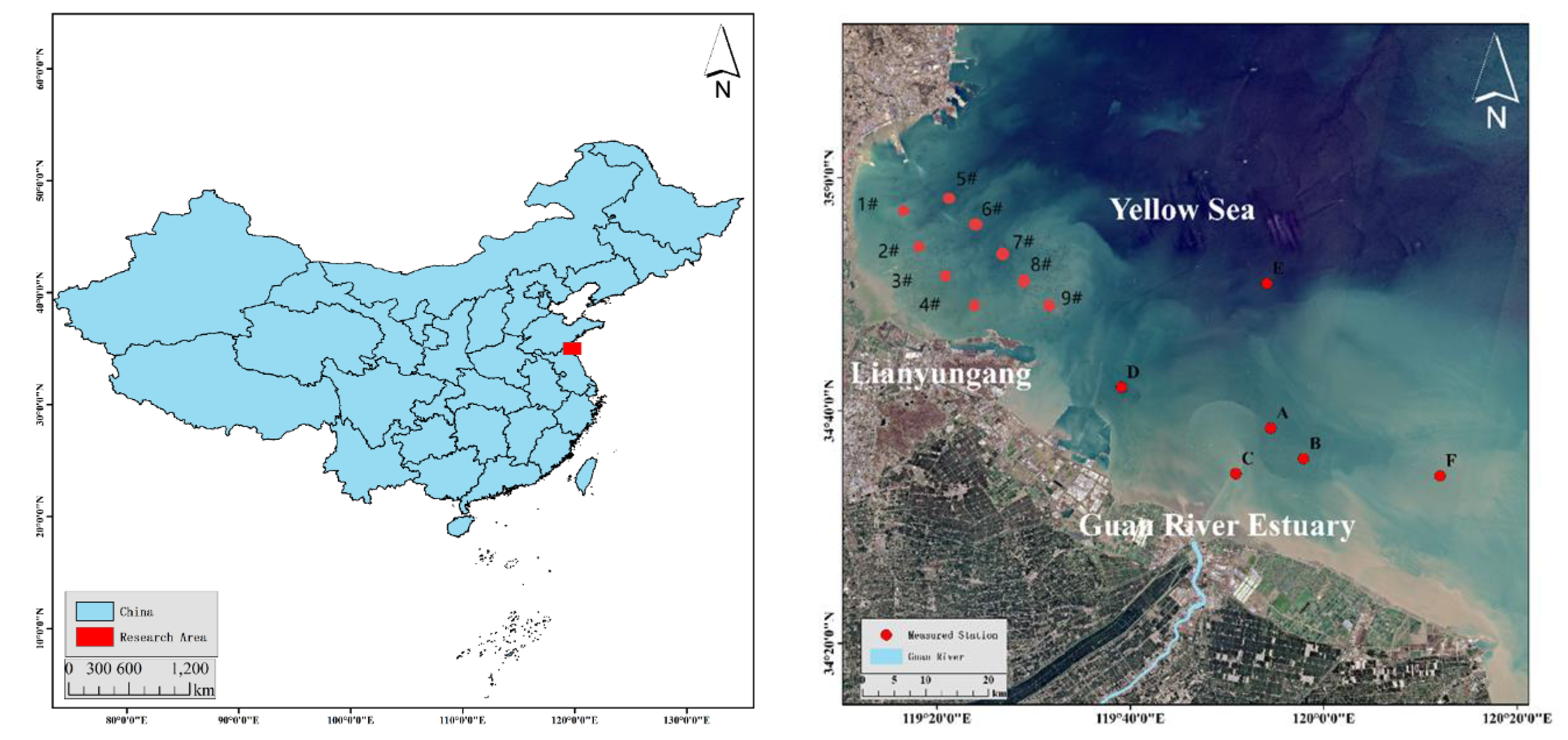
Figure 2.
Turbulent shear at Station A on April 25.
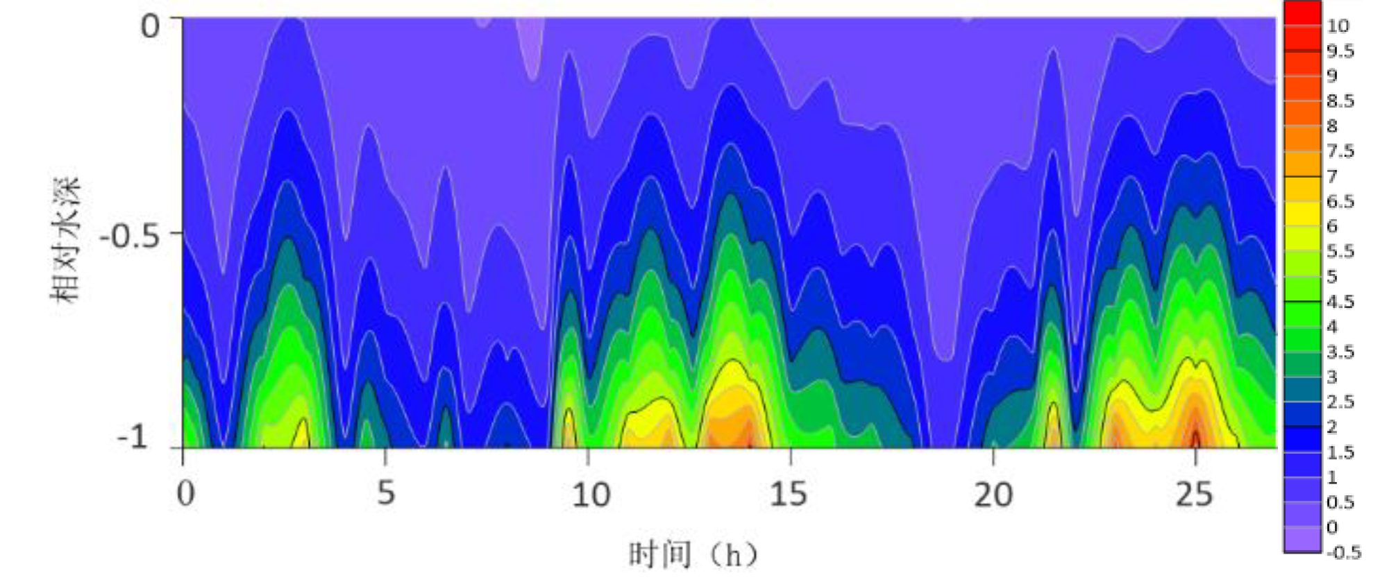
Figure 3.
Turbulent shear at Station B on April 25.

Figure 4.
Turbulent shear at Station C on April 25.
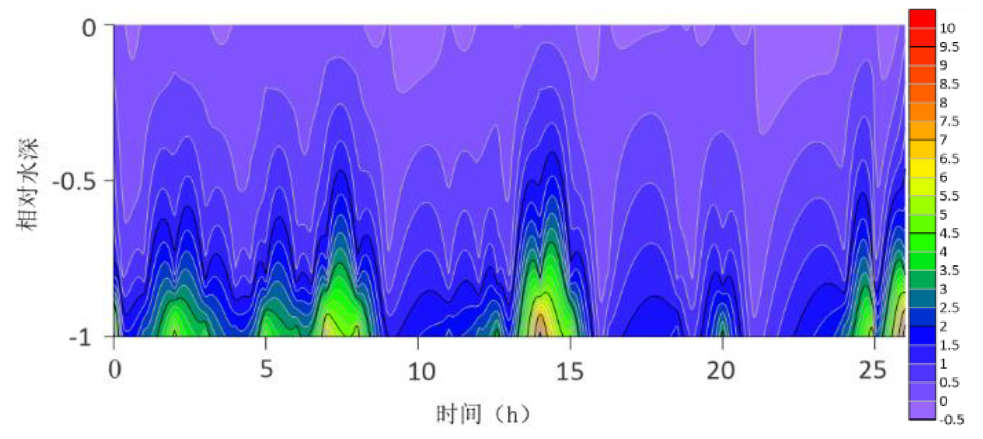
Figure 5.
Turbulent shear at Station D on April 25.
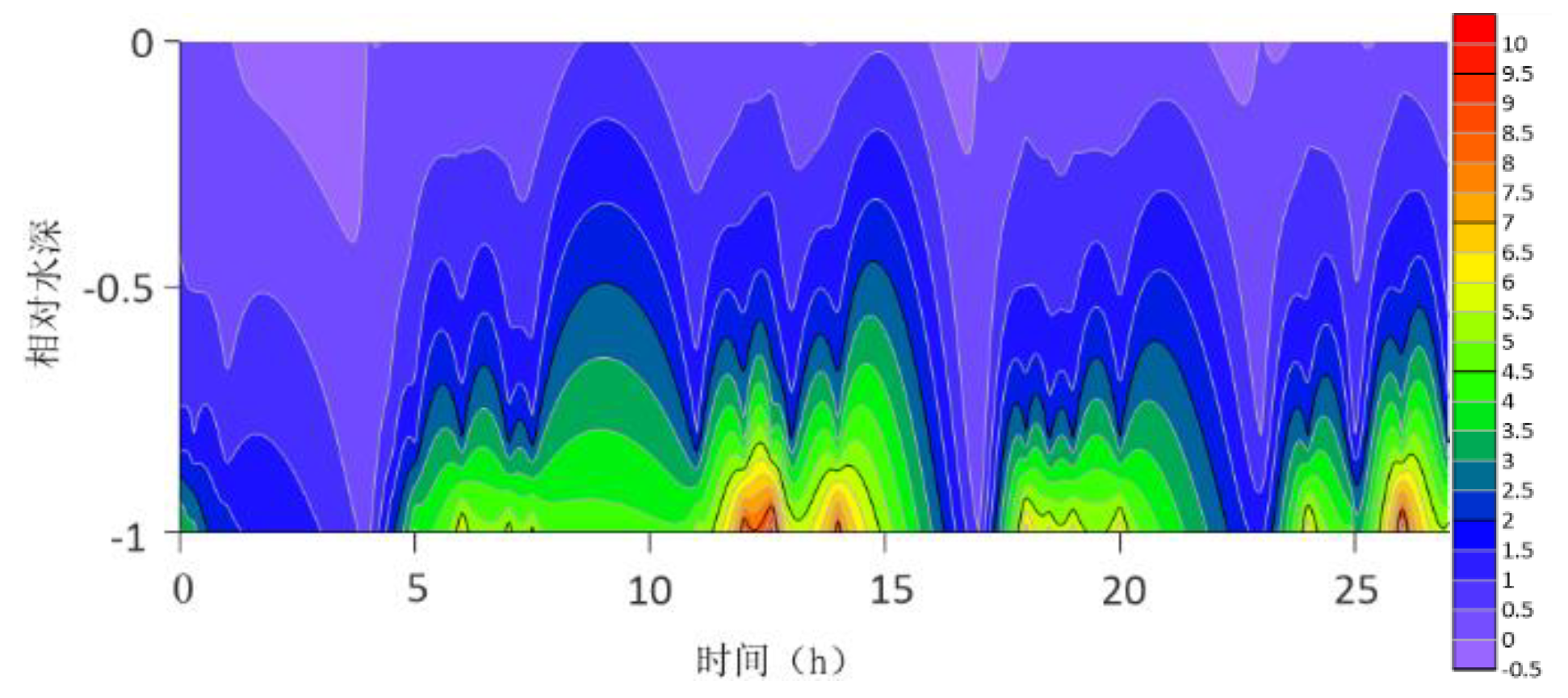
Figure 6.
Turbulent shear at Station E on April 25.
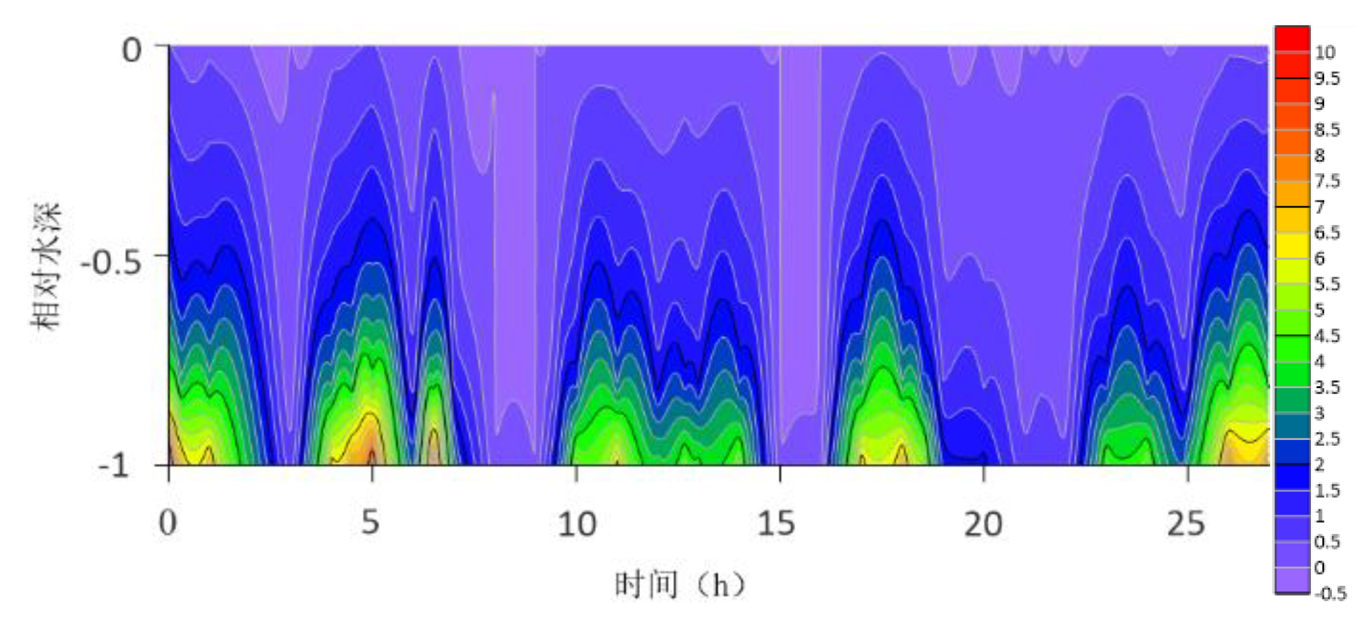
Figure 7.
Turbulent shear at Station F on April 25.
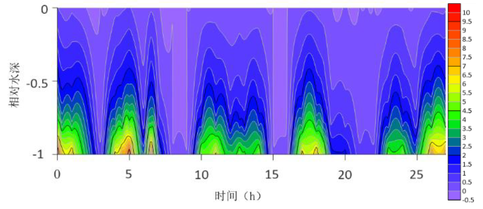
Figure 8.
Turbulent shear at Station A on April 30.
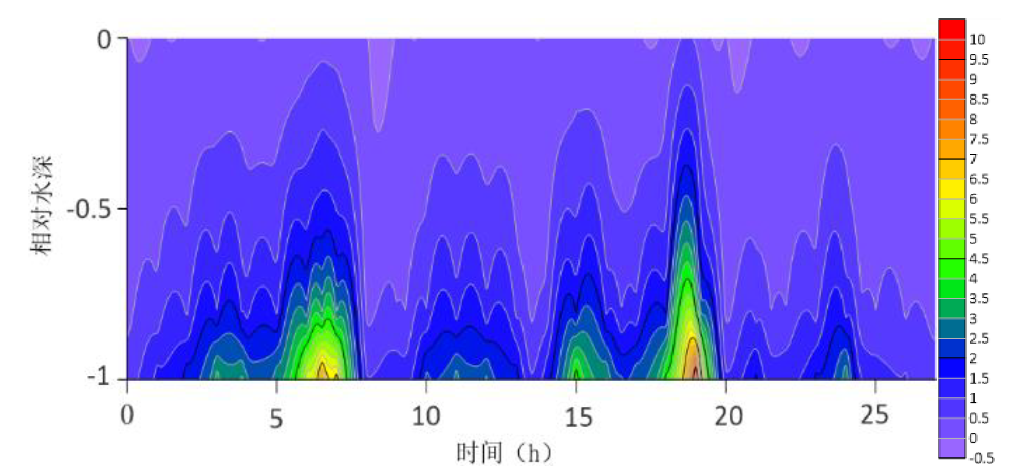
Figure 9.
Turbulent shear at Station B on April 30.
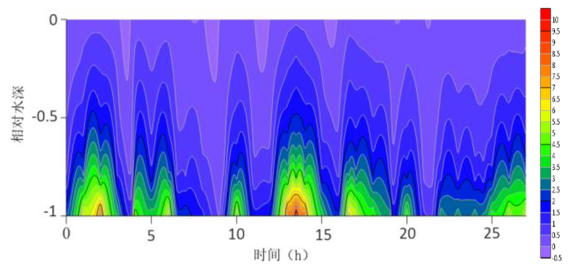
Figure 10.
Turbulent shear at Station C on April 30.
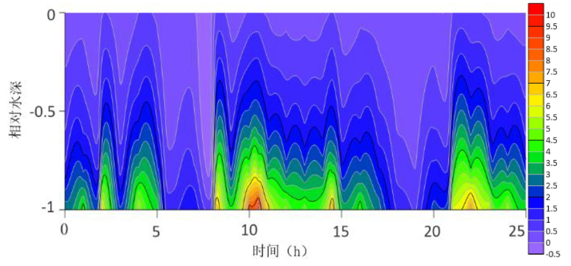
Figure 11.
Turbulent shear at Station D on April 30.
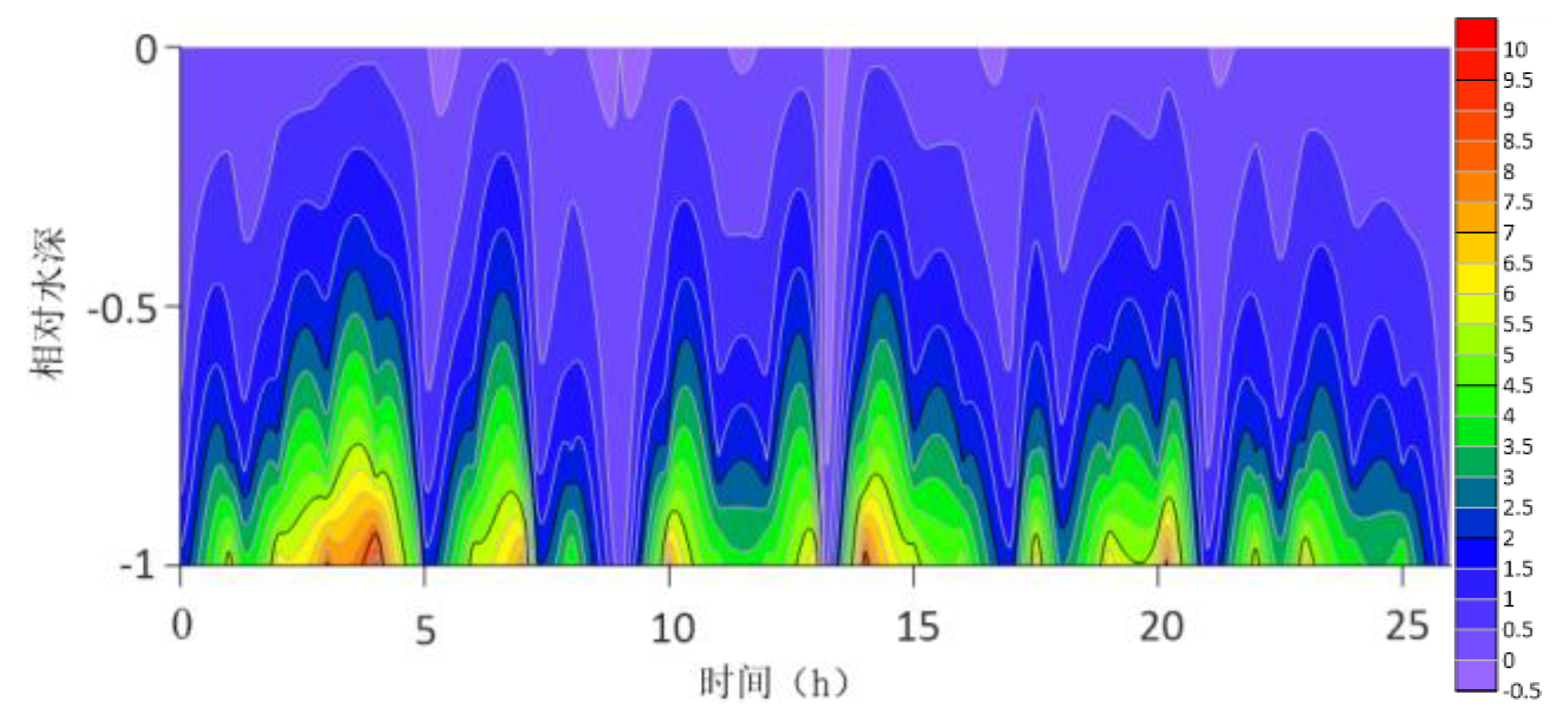
Figure 12.
Turbulent shear at Station E on April 30.
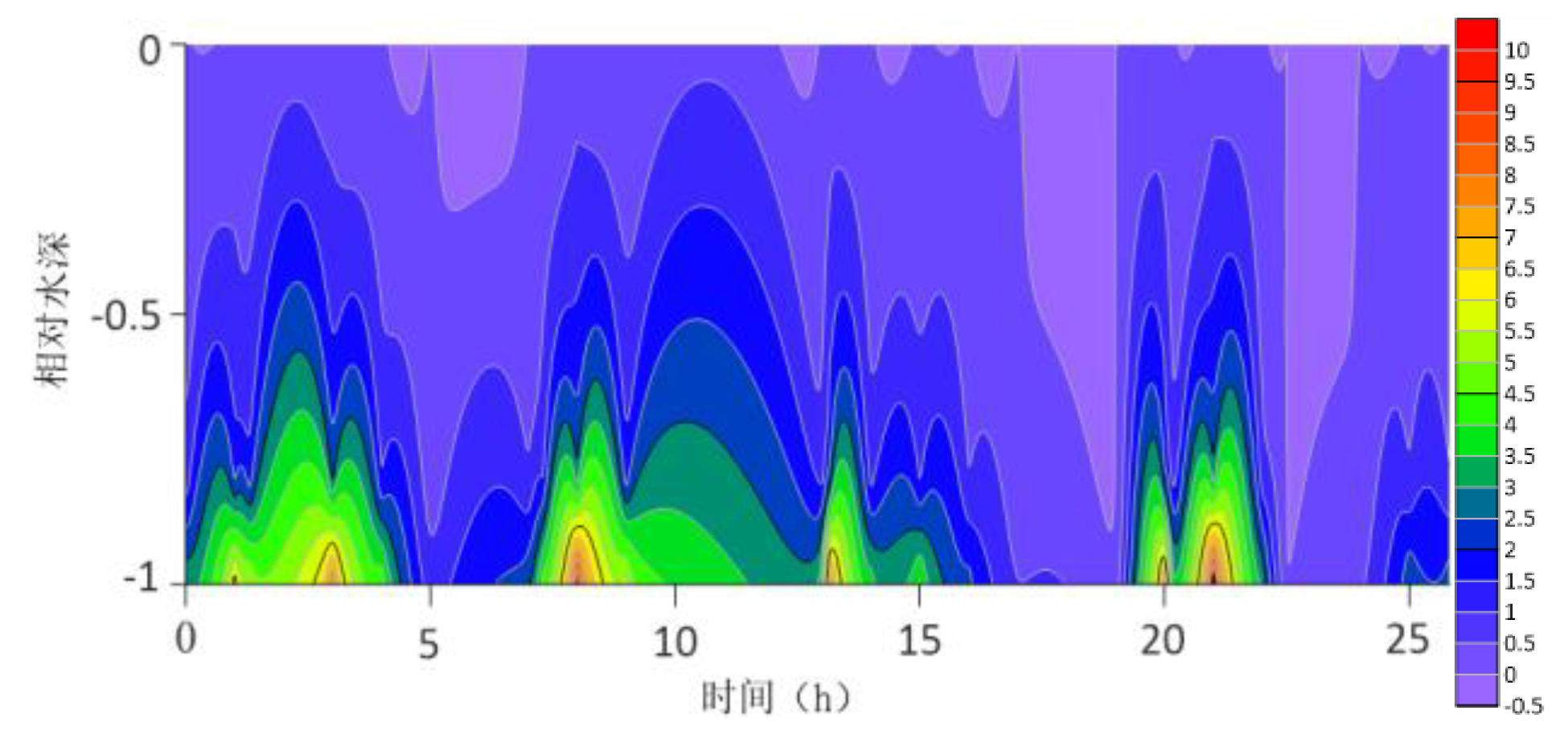
Figure 13.
Turbulent shear at Station F on April 30.
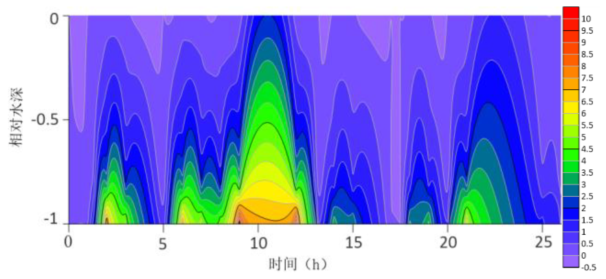
Figure 14.
Contour plot of surface sediment concentration.
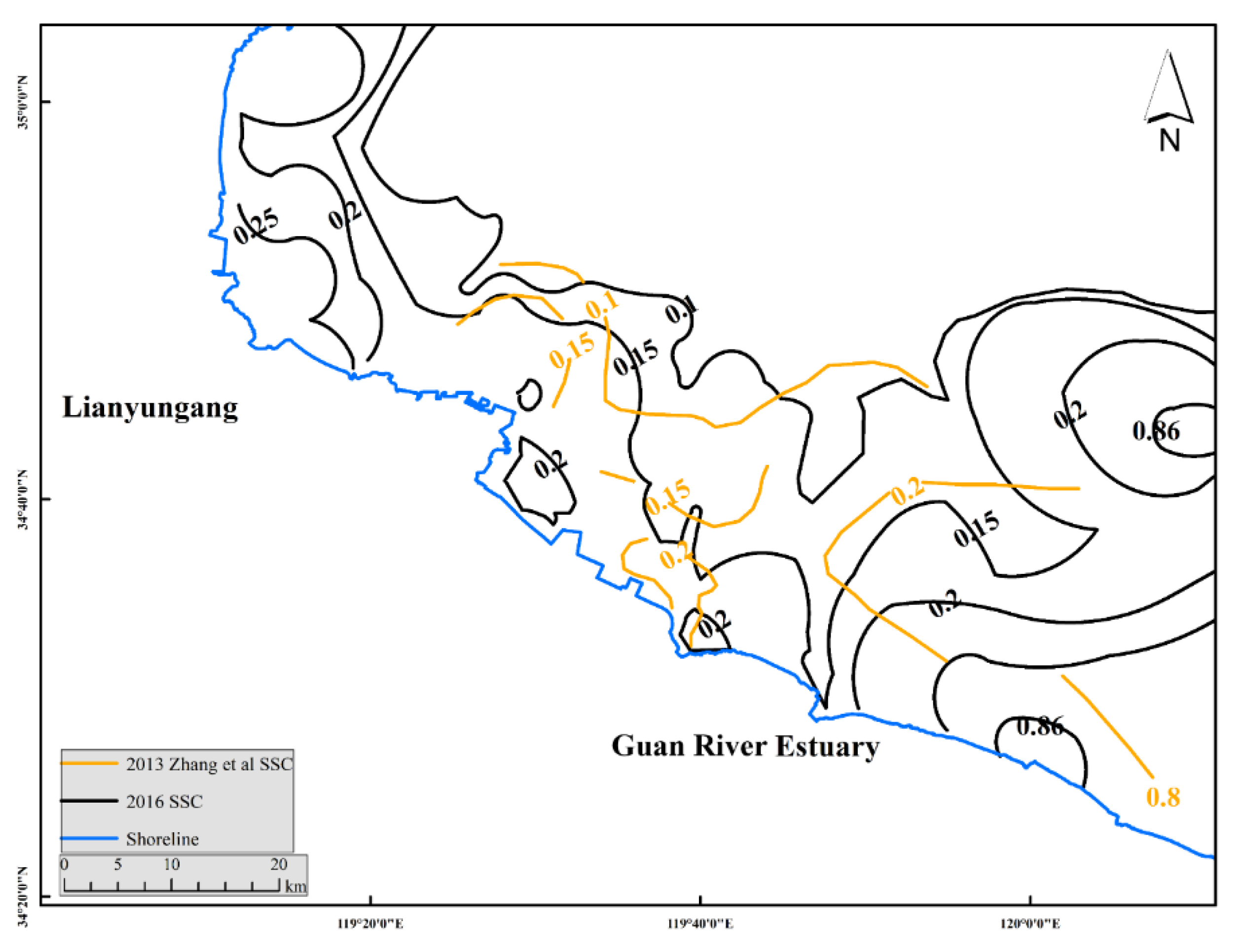
Figure 15.
Remote sensing inversion of surface sediment concentration contour map.
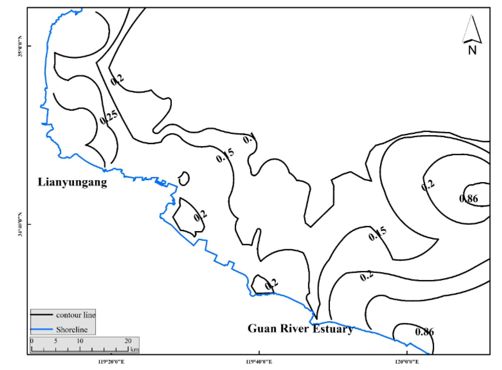
Figure 16.
Remote sensing inversion of middle sediment concentration contour map.
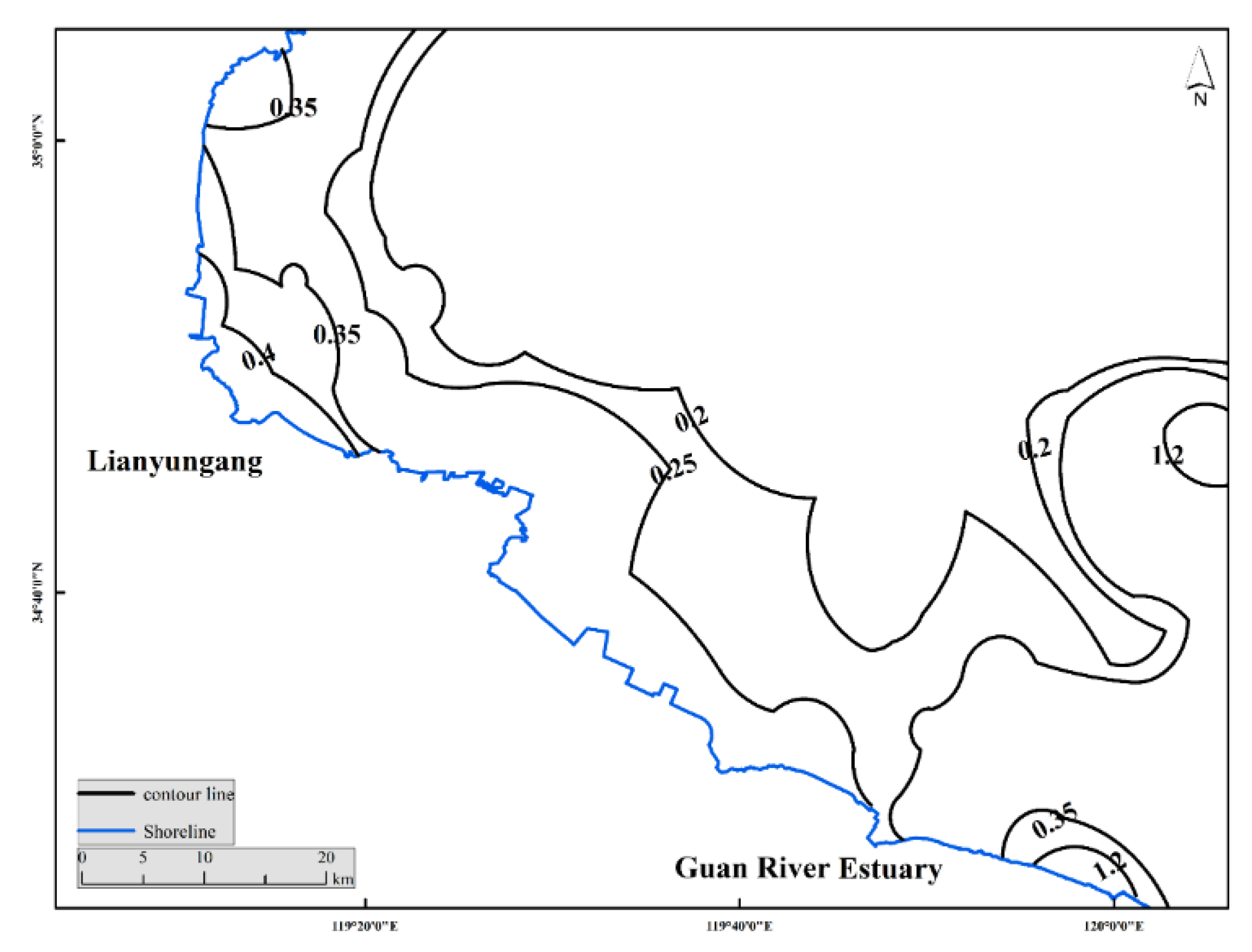
Figure 17.
Remote sensing inversion of bottom sediment concentration contour map.
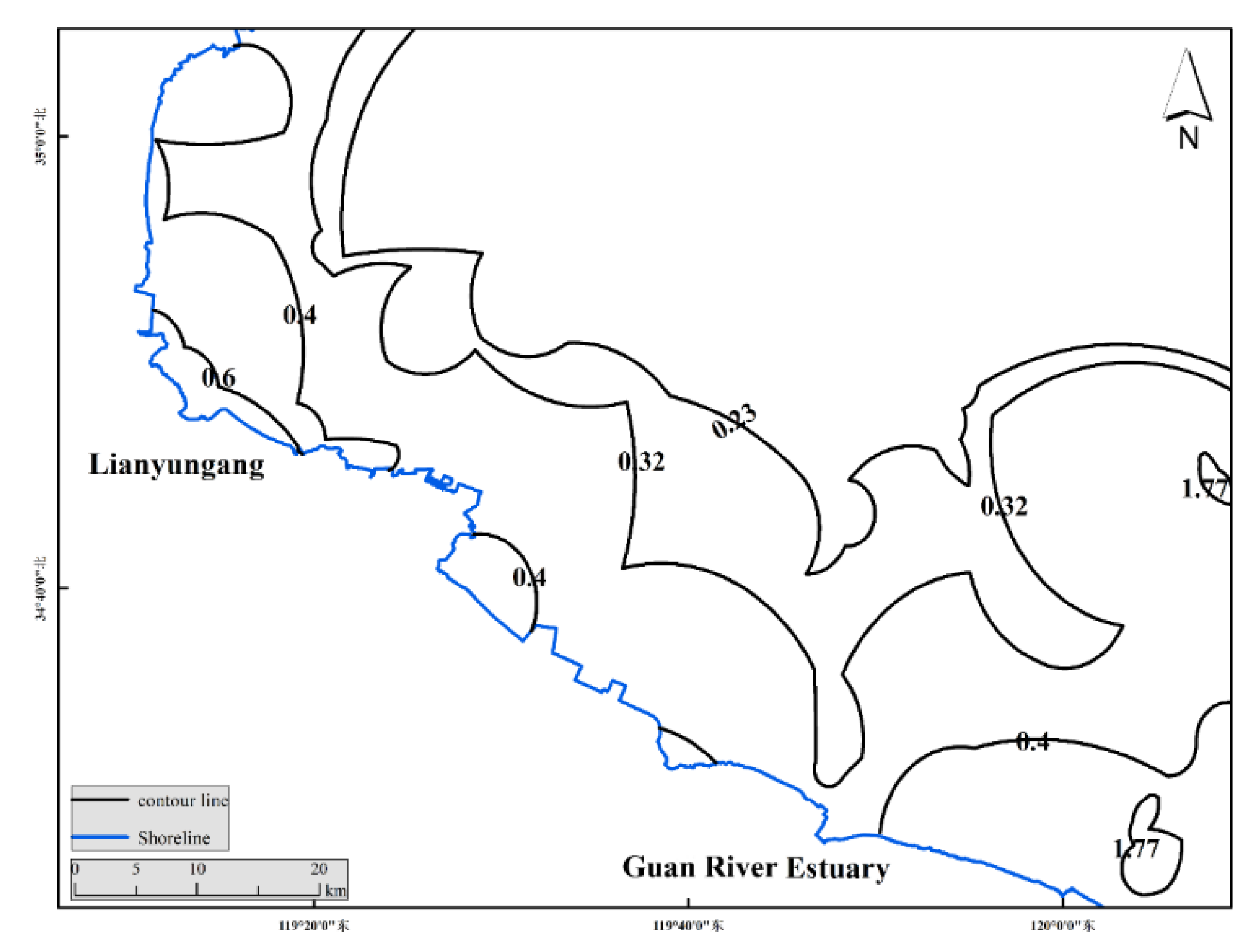
Figure 18.
The combined values of (B3+B2)/B1 band and the concentration value of suspended sediment were fitted to the trend line by a linear model.
Figure 18.
The combined values of (B3+B2)/B1 band and the concentration value of suspended sediment were fitted to the trend line by a linear model.
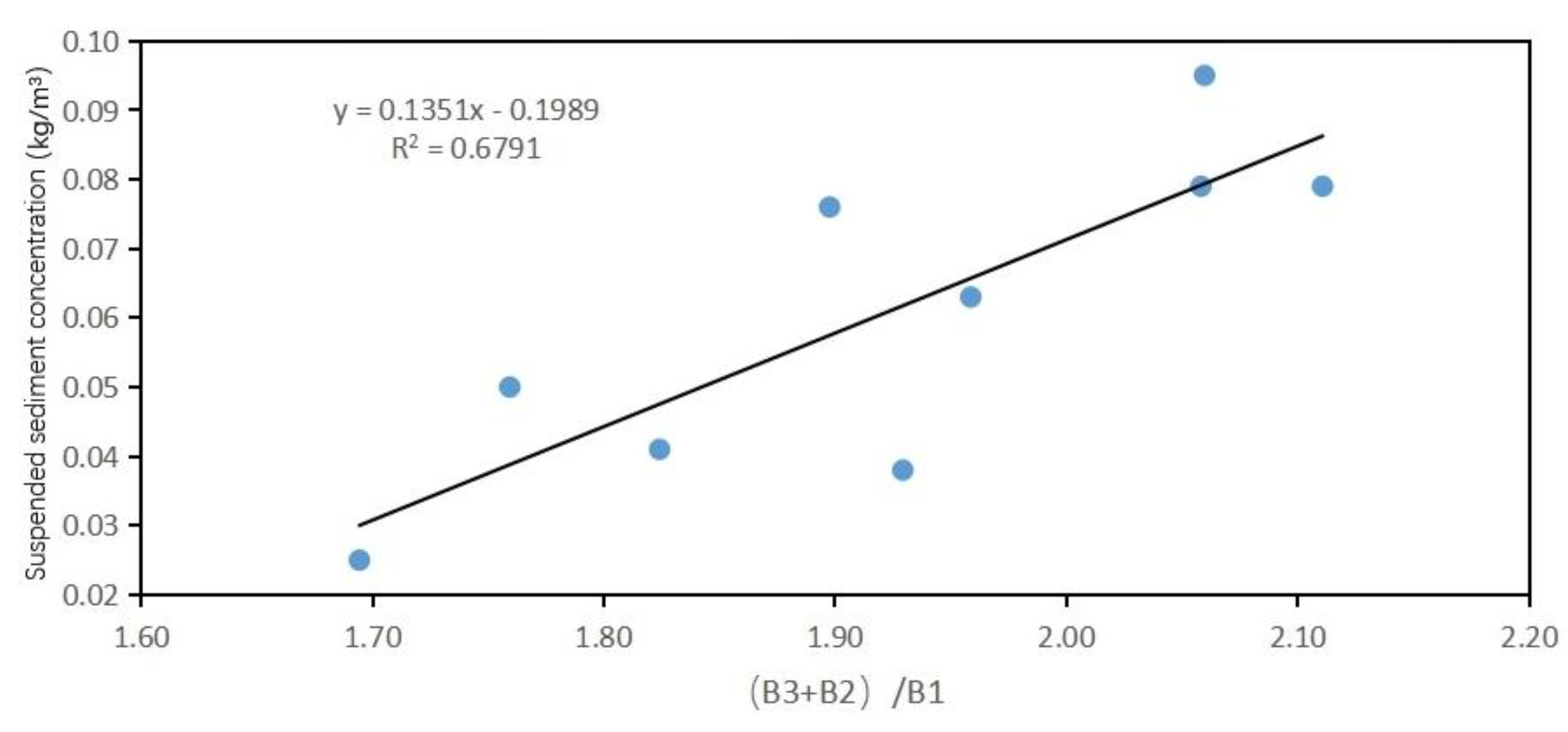
Figure 19.
The combined values of (B3+B2)/B1 bands and the polynomial model of suspended sediment concentration values fit the trend line.
Figure 19.
The combined values of (B3+B2)/B1 bands and the polynomial model of suspended sediment concentration values fit the trend line.
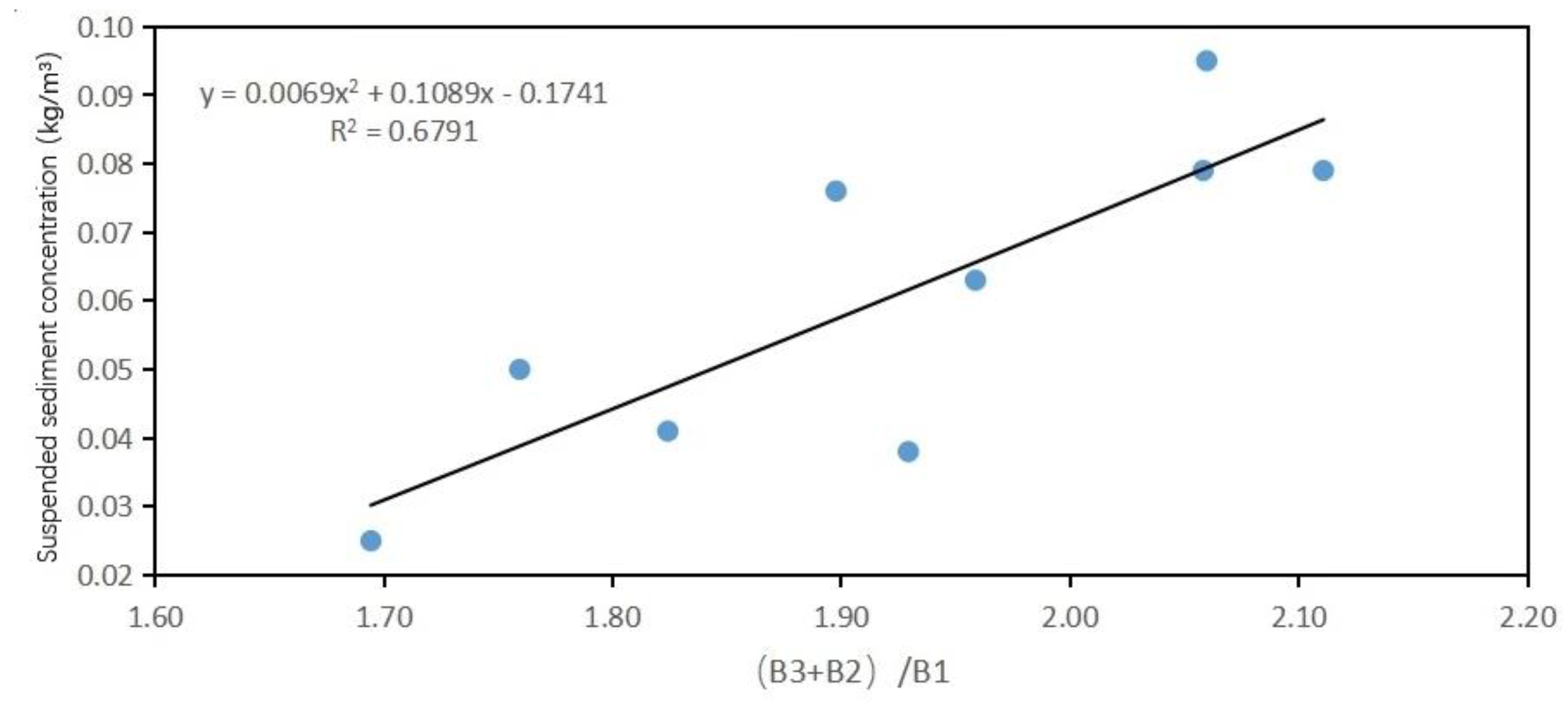
Figure 20.
The combined value of (B3+B2)/B1 band and the exponential function model of suspended sediment concentration value fit the trend line.
Figure 20.
The combined value of (B3+B2)/B1 band and the exponential function model of suspended sediment concentration value fit the trend line.
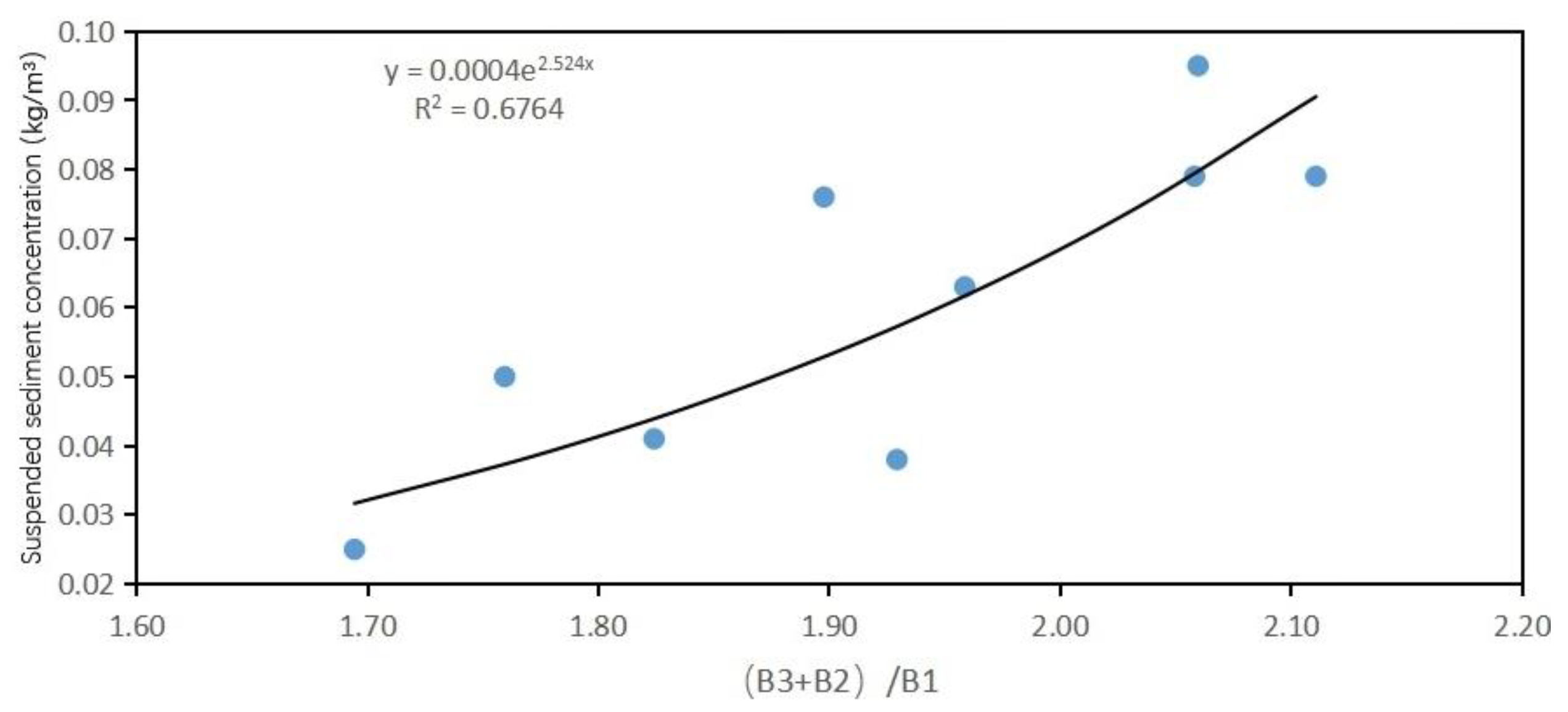
Figure 21.
The combined value of (B3+B2)/B1 band and the logarithmic function model of suspended sediment concentration value fit the trend line.
Figure 21.
The combined value of (B3+B2)/B1 band and the logarithmic function model of suspended sediment concentration value fit the trend line.
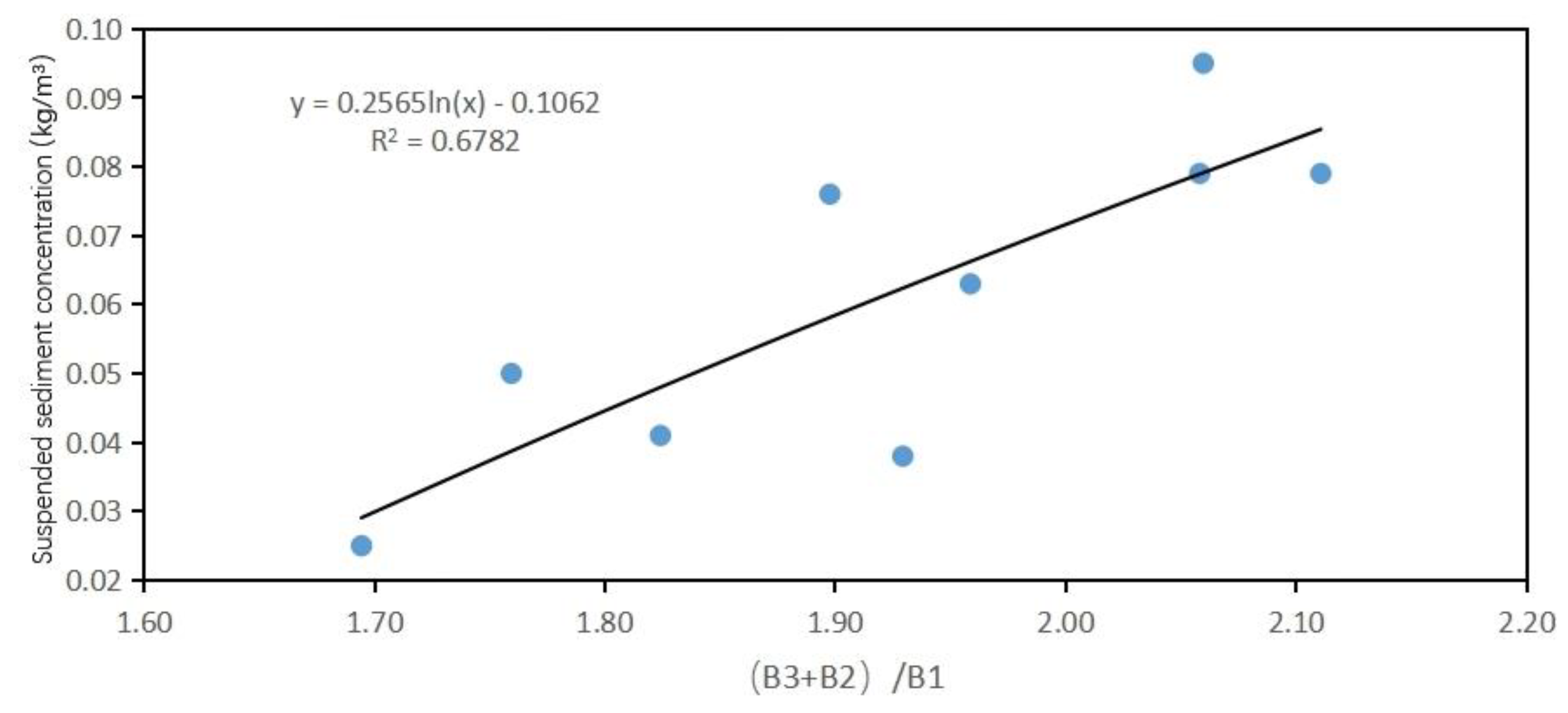
Figure 22.
Tidal variation of SSV at each station.
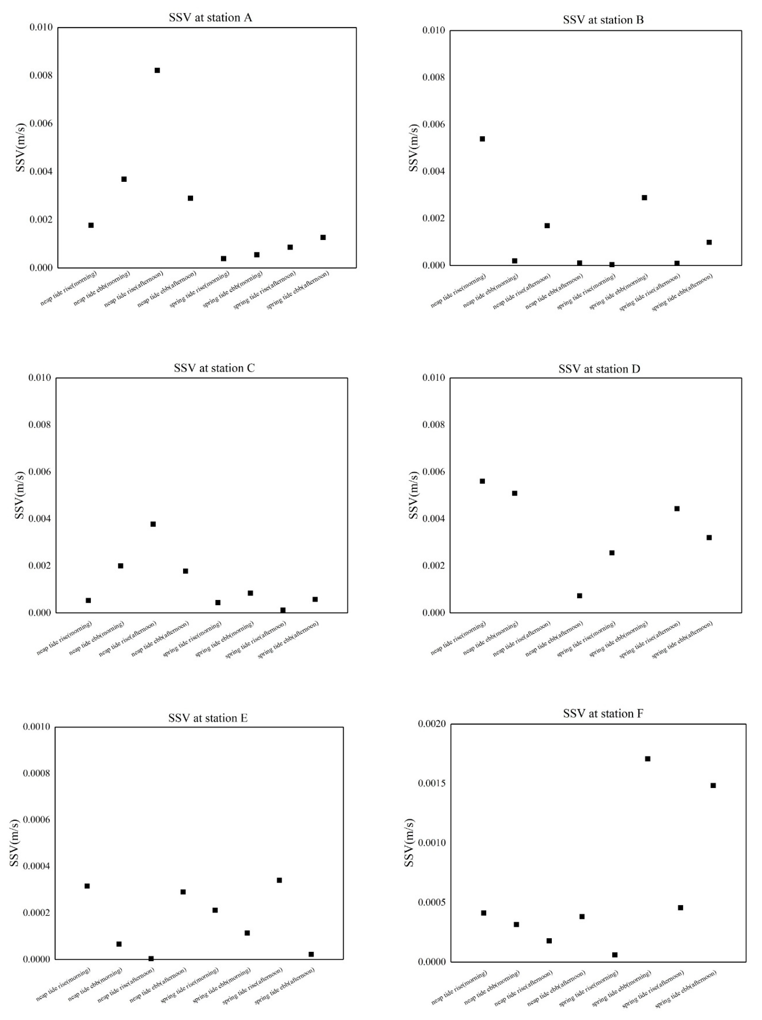
Figure 23.
The correlation between f the SSV and the SSV by fitting in spring tide period.
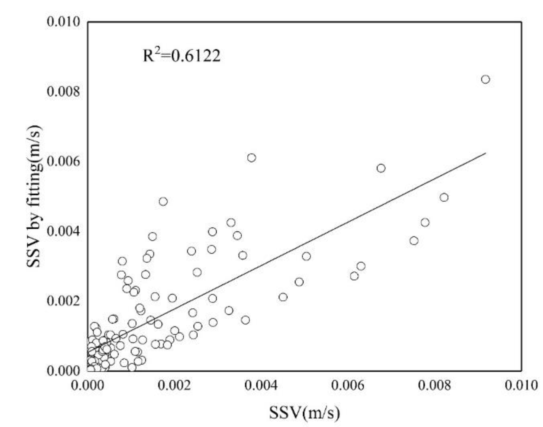
Figure 24.
The correlation between the SSV and the SSV by fitting in neap tide period.
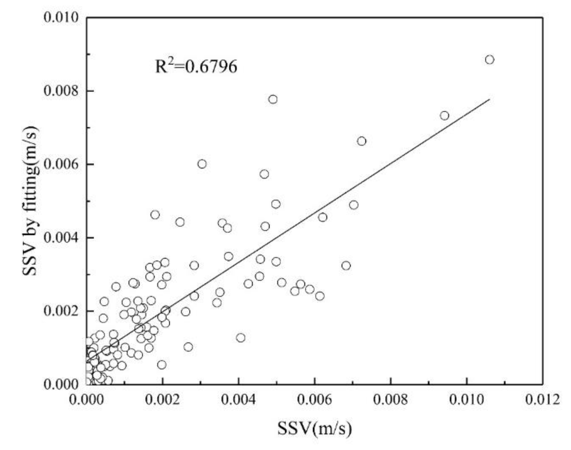
Figure 25.
The variation of SSV with SSC at station E.
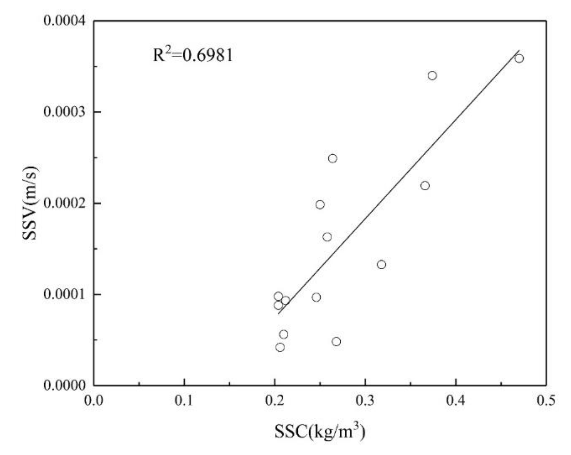
Figure 26.
The variation of SSV with SSC at station C.
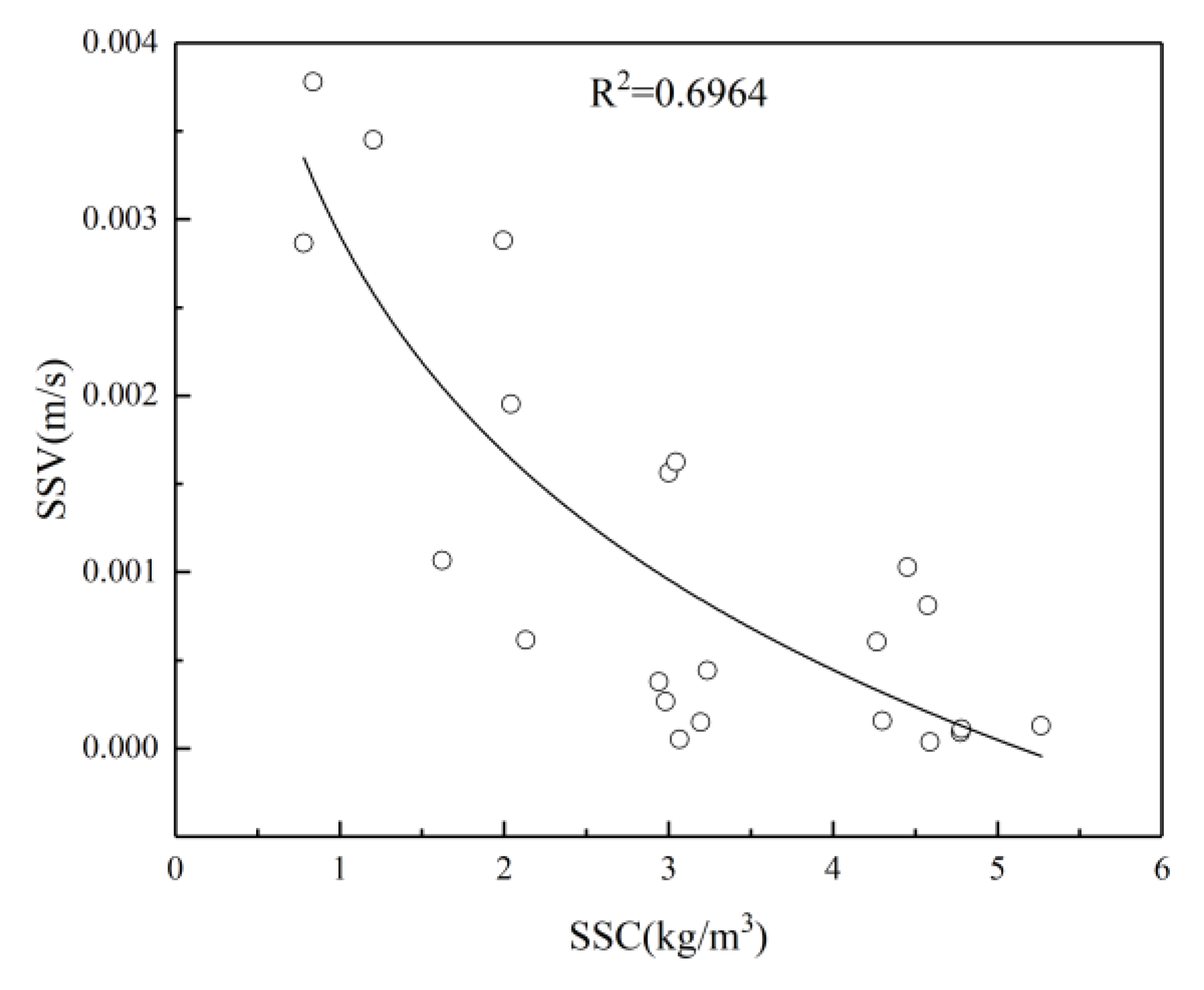
Table 2.
The time and method for obtaining sediment data.
| Study Area | Seawater Bay | |
|---|---|---|
| Number of Stations | 6 fixed observation stations | |
| Tidal Phase | Spring Tide | Neap Tide |
| Observation Date | April 25, 2016 - April 26, 2016 | April 29, 2016 - April 30, 2016 |
| Observation Period | 10:00, Apr 25, 2016 - 10:00, Apr 26, 2016 | 07:00, Apr 29, 2016 - 07:00, Apr 30, 2016 |
| Duration | 25 hours | |
| Sampling Frequency | Hourly water sampling | |
| Sampling Method | Methods varied according to water depth | |
| Parameter Measured | Suspended Sediment Concentration (SSC) | |
| Analytical Method | Filter membrane gravimetric method | |
Table 3.
Landsat 8 OLI B1, B2, B3, B4 spectral reflectance equivalent value of each measured point.
| Site | B1 | B2 | B3 | B4 |
|---|---|---|---|---|
| 1# | 0.059702 | 0.051660 | 0.061631 | 0.028897 |
| 2# | 0.062753 | 0.053403 | 0.061066 | 0.025936 |
| 3# | 0.062905 | 0.058154 | 0.071310 | 0.035601 |
| 4# | 0.068241 | 0.063388 | 0.077164 | 0.043033 |
| 5# | 0.052764 | 0.044949 | 0.047883 | 0.013292 |
| 6# | 0.069171 | 0.064092 | 0.081904 | 0.052539 |
| 7# | 0.066305 | 0.058325 | 0.069595 | 0.035689 |
| 8# | 0.062582 | 0.056905 | 0.065668 | 0.030104 |
| 9# | 0.052787 | 0.044319 | 0.045123 | 0.013339 |
Table 4.
The ratio of the equivalent reflectance values of each band of Landsat 8 OLI spectrum at each measured point.
Table 4.
The ratio of the equivalent reflectance values of each band of Landsat 8 OLI spectrum at each measured point.
| Site | B4/B3 | B4/B2 | B4/B1 | B3/B2 | B3/B1 | B2/B1 |
|---|---|---|---|---|---|---|
| 1# | 0.468875 | 0.559372 | 0.484031 | 1.193011 | 1.032324 | 0.865310 |
| 2# | 0.424718 | 0.485668 | 0.413299 | 1.143506 | 0.973112 | 0.850990 |
| 3# | 0.499235 | 0.612173 | 0.565941 | 1.226222 | 1.133615 | 0.924478 |
| 4# | 0.557674 | 0.678879 | 0.630597 | 1.217341 | 1.130763 | 0.928880 |
| 5# | 0.277597 | 0.295719 | 0.251921 | 1.065283 | 0.907508 | 0.851894 |
| 6# | 0.641478 | 0.819746 | 0.759556 | 1.277902 | 1.184072 | 0.926575 |
| 7# | 0.512806 | 0.611891 | 0.538247 | 1.193220 | 1.049611 | 0.879646 |
| 8# | 0.458423 | 0.529017 | 0.481030 | 1.153992 | 1.049315 | 0.909291 |
| 9# | 0.295621 | 0.300987 | 0.252700 | 1.018150 | 0.854813 | 0.839574 |
Table 5.
Combination values of equivalent reflectance values of each band of Landsat 8 OLI spectrum of each measured point.
Table 5.
Combination values of equivalent reflectance values of each band of Landsat 8 OLI spectrum of each measured point.
| Site | B4/(B3+B2) | B4/(B3+B1) | B3/(B2+B1) | (B4+B3)/B2 | (B3+B2)/B1 |
|---|---|---|---|---|---|
| 1# | 0.255071 | 0.238166 | 0.553433 | 1.752383 | 1.897634 |
| 2# | 0.226577 | 0.209465 | 0.525725 | 1.629175 | 1.824102 |
| 3# | 0.274983 | 0.265250 | 0.589051 | 1.838394 | 2.058094 |
| 4# | 0.306168 | 0.295949 | 0.586228 | 1.896220 | 2.059643 |
| 5# | 0.143186 | 0.132068 | 0.490043 | 1.361002 | 1.759403 |
| 6# | 0.359869 | 0.347771 | 0.614600 | 2.097648 | 2.110647 |
| 7# | 0.278992 | 0.262609 | 0.558409 | 1.805110 | 1.929258 |
| 8# | 0.245598 | 0.234727 | 0.549584 | 1.683009 | 1.958606 |
| 9# | 0.149140 | 0.136240 | 0.464680 | 1.319137 | 1.694387 |
Table 6.
Inversion model construction of the relationship between B1 band and suspended sediment concentration and its correlation coefficients.
Table 6.
Inversion model construction of the relationship between B1 band and suspended sediment concentration and its correlation coefficients.
| Band | Model | Relation | |
|---|---|---|---|
| B1 | Linear function model of one order | 0.3303 | |
| Quadratic polynomial function model | 0.3304 | ||
| Exponential function model | 0.3292 | ||
| Logarithmic function model | 0.3308 |
Table 7.
Inversion model construction of the relationship between B2 band and suspended sediment concentration and its correlation coefficients.
Table 7.
Inversion model construction of the relationship between B2 band and suspended sediment concentration and its correlation coefficients.
| Band | Model | Relation | |
|---|---|---|---|
| B2 | Linear function model of one order | 0.4653 | |
| Quadratic polynomial function model | 0.4746 | ||
| Exponential function model | 0.4533 | ||
| Logarithmic function model | 0.4577 |
Table 8.
Inversion model construction of the relationship between B3 band and suspended sediment concentration and its correlation coefficients.
Table 8.
Inversion model construction of the relationship between B3 band and suspended sediment concentration and its correlation coefficients.
| Band | Model | Relation | |
|---|---|---|---|
| B3 | Linear function model of one order | 0.5195 | |
| Quadratic polynomial function model | 0.5203 | ||
| Exponential function model | 0.5147 | ||
| Logarithmic function model | 0.5127 |
Table 9.
Inversion model construction of the relationship between B4 band and suspended sediment concentration and its correlation coefficients.
Table 9.
Inversion model construction of the relationship between B4 band and suspended sediment concentration and its correlation coefficients.
| Band | Model | Relation | |
|---|---|---|---|
| B4 | Linear function model of one order | 0.487 | |
| Quadratic polynomial function model | 0.4933 | ||
| Exponential function model | 0.4672 | ||
| Logarithmic function model | 0.4802 |
Note: In the above table, the function variable is the suspended sediment concentration (SSV), and B1, B2, B3, and B4 respectively represent the first, second, third, and fourth bands in the Landsat 8 remote sensing image data, which are the reflection values of the four different bands B1, B2, B3, and B4 read in ENVI5.2.
Table 16.
Function models with correlation coefficients higher than 0.66 and their correlation coefficients.
Table 16.
Function models with correlation coefficients higher than 0.66 and their correlation coefficients.
| Band | Relation | |
|---|---|---|
| B2/B1 | 0.66 | |
| B3/B1 | 0.6604 | |
| 0.6604 | ||
| 0.6662 | ||
| (B3+B2)/B1 | 0.6791 | |
| 0.6791 | ||
| 0.6764 | ||
| 0.6782 |
Table 17.
Regression coefficient and other related variables of fitting Equation (10).
| k | x | y | R2 | |
|---|---|---|---|---|
| spring tide | -0.55966 | -0.11049 | 0.92509 | 0.6122 |
| neap tide | -1.00776 | -1.3826 | 0.83908 | 0.6796 |
Disclaimer/Publisher’s Note: The statements, opinions and data contained in all publications are solely those of the individual author(s) and contributor(s) and not of MDPI and/or the editor(s). MDPI and/or the editor(s) disclaim responsibility for any injury to people or property resulting from any ideas, methods, instructions or products referred to in the content. |
© 2026 by the authors. Licensee MDPI, Basel, Switzerland. This article is an open access article distributed under the terms and conditions of the Creative Commons Attribution (CC BY) license.
Copyright: This open access article is published under a Creative Commons CC BY 4.0 license, which permit the free download, distribution, and reuse, provided that the author and preprint are cited in any reuse.


