
Submitted:
30 December 2025
Posted:
30 December 2025
You are already at the latest version
Abstract
Understanding how socio-economic and demographic factors influence electric vehicle (EV) adoption is crucial for designing equitable policies that support the global transition to sustainable transportation. While EV uptake is rising worldwide, adoption patterns often reflect existing social and economic inequalities, with higher-income communities more likely to benefit from emerging technologies. Addressing these disparities is essential to ensure an inclusive transition. This study focuses on Australia, using New South Wales (NSW) as a case study to examine how socio-economic and demographic characteristics shape EV adoption across different postcodes. A cross-sectional analysis was conducted using 2021 data from the Australian Bureau of Statistics (ABS) census and EV registration records. Postcodes were categorised based on EV uptake levels, and Ordinary Least Squares (OLS) regression models were applied to identify key influencing factors. The results show a strong correlation between higher EV adoption rates and areas with greater wealth and population density. In contrast, factors such as marital status, dwelling structure, driving habits, vehicle ownership, and younger age showed no significant association with uptake. These findings highlight the need for targeted policy interventions to bridge socio-economic gaps in EV adoption. Expanding charging infrastructure and providing financial incentives in lower-income areas could promote more inclusive access to EV technology. Moreover, aligning EV adoption strategies with broader environmental and transportation policies can further accelerate Australia’s energy transition. This study emphasises that a more equitable approach to EV adoption not only enhances environmental outcomes but also supports a fair and sustainable transportation future for all communities.
Keywords:
electric vehicle
; adoption
; socio-economic analysis
; demographic analysis
1. Introduction
Globally, the transportation sector is a major contributor to greenhouse gas emissions, largely driven by internal combustion engine (ICE) vehicles [1]. As countries seek pathways to decarbonize and meet international climate commitments, electric vehicles (EVs) have emerged as a promising solution [2]. Supported by government incentives, technological progress, and global market shifts, EVs are increasingly positioned as a cornerstone of sustainable mobility strategies [1]. With an ever-growing need to reduce greenhouse gas (GHG) emissions and combat climate change, society is becoming increasingly conscious of the environmental impact our species is making on our planet. Due to innate and unavoidable byproducts of human living, greenhouse gas emissions have been accelerating the weather phenomenon more commonly known as climate change, particularly since the age of the Industrial Revolution. According to the IPCC, global temperatures have risen by since that period, largely driven by the excessive manipulation of hydrocarbons. Furthermore, if current temperature rise trends are to continue, we are likely to pass the critical threshold by the early 2030s, as highlighted by [3]. This global climate change contributes to the increase in extreme weather events, such as bushfires, flooding, cyclones, and biodiversity loss due to abnormal rises in sea levels. Hence, it is crucial for the future well-being of humanity that measures be adopted to reduce greenhouse gas emissions and mitigate the effects of climate change. To address these pressing environmental challenges, consideration is now given to how emerging technologies, particularly electric vehicles, can help address them.
Building on the urgency to address climate change, attention has turned to the role of innovative transport solutions and policy enablers. With the continuing interest in innovative technologies, the environmental challenge has provoked capable populations to develop workable solutions. The combination of these two factors, the need to combat climate change and the constant drive for technological advancements, drives the search for cleaner modes of transportation that outperform traditional ICE vehicles. Electric Vehicles (EV) are a promising candidate for this role, producing zero tailpipe emissions, reducing dependency on fossil fuels, and standing at the forefront of current automotive innovation. Nations such as Norway and the United Kingdom, through smart policymaking, have incentivised EV adoption, achieving rates as high as 75% of new sales in Norway in 2020. In contrast, in Australia—the country of concern in this paper—the EV market remains in its infancy, comprising only 8% of new vehicle sales in Q2 of 2024, with hybrids (a combination of ICE and EV) surpassing it at 15% [4]. Accordingly, this paper investigates how socio-economic and demographic characteristics shape electric vehicle adoption in Australia, focusing on New South Wales (NSW) as a case study, to better understand how policy measures can promote a more equitable transition to sustainable transportation. To contextualise the analytical framework and research focus, Figure 1 presents a conceptual overview of the study context, including the data sources, socio-economic and demographic factors, analytical approach, and policy-relevant outcomes examined in this paper.
Understanding who adopts new technologies first is critical for effective policy interventions aimed at broader uptake. Early adopters play a crucial role in the spread of new technologies, often serving as catalysts within the Diffusion of Innovation (DOI) theory. Proposed by Everett Rogers in 1962, this theory explains how, why, and at what rate new ideas and technologies spread through cultures, categorising adopters into innovators, early adopters, early majority, late majority, and laggards [5]. Early adopters are typically a small but influential group who are keen on trying new products and are perceived as opinion leaders in their social networks. Their enthusiasm and willingness to embrace innovation influence the early majority, creating momentum toward wider acceptance. Studies also reveal that early adopters are generally more affluent, better educated, and possess a higher tolerance for risks compared to later adopters [6]. In the context of electric vehicles, early adopters are often environmentally conscious individuals with a strong interest in technology, who value sustainable and innovative products despite higher costs [7]. While these early adopters help initiate EV uptake, broader socio-economic parameters can impede mainstream diffusion, leading to a deeper elaboration of socio-economic barriers against EV uptake.
The challenging adoption of EVs in NSW indicates a need for more targeted policies that address unique geographic and socio-economic disparities. DOI provides a useful framework for understanding how income, education, and exposure to new technologies impact EV adoption. Individuals are more likely to adopt new technologies if they perceive them to be compatible with their lifestyles and observe others in their community doing the same. Nonetheless, high initial costs remain a primary barrier. Even though EVs offer lower long-term operating costs, the upfront price still dissuades many buyers, particularly when compared to ICE vehicles [8]. Income disparities in NSW compound this issue, restricting EV ownership largely to higher-income households [9]. Moreover, the longer payback period, often 5–8 years, means consumers may prioritize immediate affordability [10], and current incentives in NSW, although helpful, are modest relative to global standards [11]. While these economic obstacles are significant, it is also important to study the availability of charging infrastructure and geographic considerations for a more comprehensive understanding of the EV uptake. A well-established charging network is essential for EV adoption, as it directly affects convenience and reduces range anxiety”, the fear of running out of power without access to charging stations [12]. Urban areas in NSW, such as Sydney, typically have more charging stations, which aligns with the higher concentration of EVs in these regions. However, in rural and remote areas, where distances are greater and public transportation less accessible, charging infrastructure remains sparse, further discouraging potential EV buyers. Establishing stations in sparsely populated regions requires significant investment, and in those areas, financial returns are lower due to reduced EV ownership and use [13]. Consequently, the private sector is less incentivised to build infrastructure there, relying instead on government support. Moreover, this infrastructure gap” can create a cycle of low demand and limited investment [14]. To contextualize these findings and provide a focused application, we consider the case of New South Wales, Australia.
In Australia, transportation accounts for 19% of the country’s total GHG emissions—85% of which stems from road transport. As such, in order to reach the ambitious goals set by the NSW government to achieve net zero emissions by 2050, the uptake of EVs can be of significant help. The NSW Electric Vehicle strategy, curated by the state government, outlines various initiatives aimed at making EVs more accessible to the general public. Such incentives include a $3,000 rebate, stamp duty exemptions, a $171 million investment in charging infrastructure, and a $105 million program established to encourage local businesses to convert their fleets to EVs. However, despite these policy efforts, EV market penetration in NSW remains limited, possibly due to high upfront costs, limited model availability, and restricted charging infrastructure. Some of the key factors that shape the likelihood of EV uptake might likely be the intricate interplay of socio-economic and demographic influences. Previous studies have shown that early adopters of EVs in Australia are primarily high-income individuals with tertiary education located in urban areas, while outer suburban and rural areas face greater adoption challenges [15], exacerbated by a lower average income and less developed infrastructure [16]. This complex landscape calls for deeper inquiry into how socio-economic realities and emerging technologies converge, setting the stage for a closer look at early adopters and their role in NSW.
For this purpose, this study employs an OLS regression framework to quantify the significance of socio-economic, geographic, and infrastructural factors in fostering EV uptake. OLS regression is a commonly used statistical tool in socio-economic research for exploring how various socio-economic variables impact dependent outcomes such as income, educational attainment, and community development [17]. OLS regression helps to quantify relationships between a dependent variable and one or more independent variables by minimising the sum of squared residuals, thereby ensuring that the resulting regression line fits as closely as possible to observed data points. This method is widely applied in policy and economic studies due to its simplicity and interpretability. For instance, studies examining regional development frequently leverage OLS to assess the socio-economic impacts of rural infrastructure or high-speed rail networks, enabling insights into community growth and quality of life improvements [18,19]. Nevertheless, OLS does have certain limitations. It assumes linearity, which can be problematic when socio-economic relationships are more complex or non-linear, and it can be sensitive to multicollinearity, which may distort the accuracy of the model’s results [20]. To mitigate such issues, advanced or alternative methods, such as structural equation modeling (SEM), are sometimes employed, particularly when analyzing multi-dimensional impacts like those seen in ecotourism or economic growth [21]. Given these analytical considerations, a cross-sectional snapshot in previous time data, e.g., 2021, is especially valuable for capturing the immediate state of EV adoption in NSW.
Cross-sectional studies are pivotal in socio-economic research as they provide a snapshot of specific population groups at a single point in time, allowing one to understand socio-economic conditions, behaviours, and outcomes [18]. By capturing variations across demographics, cross-sectional analyses facilitate insights into the socio-economic dynamics that shape community development and policy efficacy [22]. For this paper, focusing on data from 2021 offers a concise view of the factors affecting EV uptake prior to significant policy changes or broader market shifts in subsequent years. Building from this perspective, it is now possible to outline the primary aims and objectives of this study and how they guide the analysis.
This report aims to explore the socio-economic and demographic dimensions of EV adoption in NSW, Australia for the year 2021, providing insights into the statistically significant characteristics of POAs that affect varying adoption rates. As such, this cross-sectional study seeks to address the question: What are the key socio-economic and demographic factors that, in the context of NSW, are associated with an increase in EV registration numbers? Based on previous literature and thoughtful consideration, the hypothesis is that increased population density, higher wealth, and higher education levels will each positively contribute to an increase in EV registrations within a postcode area. By answering this question, additional concerns can be addressed, namely, which factors might be hindering broader EV uptake and how policies or smart infrastructure planning could be curated to enhance accessibility and drive adoption. This will be achieved by quantifying and comparing the socio-economic profiles of high and low EV adoption areas, examining factors such as income, education level, and housing type, and identifying significant disparities that may point to underlying socio-economic barriers. In turn, the research seeks to support targeted policy and infrastructure strategies that can accelerate EV adoption equitably across diverse NSW communities while also contributing to the broader understanding of how socio-economic variables drive technology adoption in emerging markets within the scope of the study as stated as follows. Having established these aims, we now consider the scope and limitations that frame the boundaries of this study.
Since the study relies solely on socio-economic and demographic variables from 2021, and EV registration data up to 2017, it offers only a limited snapshot of the associations for that period. Consequently, this single-year perspective constrains the findings from offering longitudinal insights into evolving EV adoption patterns. Additionally, this study does not address the direct influence of proximity to charging infrastructure, because high EV registrations often trigger further infrastructure development, making it difficult to disentangle cause-and-effect relationships. By focusing on socio-economic and demographic factors, some spatial or infrastructural dynamics may, therefore be overlooked. Moreover, broader elements such as environmental attitudes, perceived innovation risk, lifestyle habits, and social media behaviours (as discussed in [23] and the Diffusion of Innovation Theory) are not captured here, primarily due to limitations in census data. Although such factors could provide deeper insight, their quantification remains out of scope for this research. Within these boundaries, the next sections present the detailed methodology, empirical results, and policy implications emerging from this cross-sectional examination. The remainder of this paper is structured as follows. Section 2 (Data-Driven Approach to Analysing EV Adoption Factors) details the OLS regression model and clarifies the key socio-economic and demographic variables employed. Section 3 (Empirical Insights into EV Uptake in NSW) presents the main findings and discusses their implications in the context of socio-economic disparities and infrastructure constraints. Section 4 (Conclusions and Policy Recommendations for EV Growth) synthesizes these findings and suggests pathways for policymakers and stakeholders. The Appendices provide extended results (Appendix A) and additional spatial analyses (Appendix B).
2. Materials and Methods
In this section, the research design, data collection, and analytical procedures used in this study are outlined. The methods used are presented step-by-step so that they can be easily replicated, while providing increased clarity at the same time.
2.1. Research Design
This study analyses EV adoption in NSW at a postcode level, using postal areas (POAs) as the geographical unit. The dependent variable is the the number of electric vehicle registrations count captured up to 2021. This measure provides insights into the early adoption patterns and spatial distribution of EV uptake across NSW, aligned with similar studies conducted on technology adoption in Australia [15].
The independent variables in the analysis are drawn from the Australian Bureau of Statistics Census data for year 2021. Variables that relate to economic status, social influence, and accessibility to technology were carefully selected based on the established connections to technology patterns, guided by the Diffusion of Innovation Theory [23]. The relevance of each variable is statistically assessed through the use of regression analysis.
The study encompasses 673 postcodes across NSW with available EV registration data for 2021. This sample size provides adequate statistical power for multiple regression analysis. Based on the guideline of at least 10-15 observations per predictor variable [24], our sample of 673 postcodes supports models with up to 45-67 independent variables, well above the 8 variables retained in our final model, ensuring robust statistical inference.
2.2. Dependent Variable
The dependent variable for this research is sourced from the NSW Government Roads and Maritime Services, hosted by the Institute of Sustainable Futures at UTS, and is a byproduct of a project initiated by the Electric Vehicle Council ([25]). The data contain NSW EV registrations organised by postcode for each year between 2017 and 2021. Other information, such as the vehicle model, was captured as well in the data model. Considering that this is a study of identifying socio-economic factors associated with residential EV adoption, only private EV registrations were included. The commercial and fleet vehicles were not included in the analysis. By selecting only private registrations, the dataset ensures that an accurate measure of EV adoption within the residential context is observed.
2.3. Independent Variables
The independent variables were selected based on their alignment with DOI and their prevalence in other EV studies. Socio-economic census data for 2021 were obtained from the Australian Bureau of Statistics (ABS) dataflow system. Census data indicators include age, income, registered motor vehicles per dwelling, rent per dwelling, mortgage per dwelling, occupation, dwelling type, percentage of year 12 completion, and percentage in education older than the age of 20—all aggregated at the POA level. The significance of these variables is assessed through statistica relevance as measured in regression analysis. Various precautions in selecting these indicators were taken to reduce multicollinearity and minimize categorical variables.
2.4. Statistical Analysis
Regression analysis was employed to determine the relationship between EV uptake and the various socio-economic variables considered. This method determines the influence that one or more independent variables has on the dependant variable, thus facilitating the understanding of statistically significant socio-economic variables with EV adoption at the POA level. In the analysis presented herein, the regression model follows the equation:
where: y is the dependent variable (EV registrations); x is the independent variable (predictor), is the intercept, is the slope coefficient and is the error term.
The data analysis follows a structured, multi-step process to ensure accuracy and reliability of both the data input and the results. Figure 2 outlines the main stages after performing literature and defining objectives of the study, starting with data collection, preparation, cleaning, model specification, testing and finally, validation. Having a structured approach allows for repeatability of the analysis, a consistent processing of the various socio-economic variables, and a methodical handling of potential multicollinearity. Steps were incorporated to cross-check model outputs against input variables, ensuring that the results were both valid and aligned with the research objectives.
Additionally, diagnostic checks, such as the residual analysis and the Variance Inflation Factor (VIF) tests, were performed to validate assumptions made by the regression model and to mitigate error, if needed. In all, the prime objective of this methodical approach is to support the production of reliable insights into the socio-economic drivers of EV adoption across NSW.
The fourteen-step process is organized into six sequential phases, as illustrated in Figure 2.
- Phase 1: Data Acquisition (Steps 1-2) – Collection and geographic alignment of data from multiple sources
- Phase 2: Data Preparation (Steps 3-5) – Processing, filtering, and aggregation of socio-economic indicators
- Phase 3: Variable Specification (Steps 6-8) – Standardization and selection of analysis variables
- Phase 4: Model Estimation (Steps 9-10) – Regression analysis and initial robustness assessment
- Phase 5: Diagnostic Testing (Steps 11-13) – Validation of model assumptions and variable significance
- Phase 6: Interpretation (Step 14) – Analysis of results and policy implications
The following paragraphs detail each step within this framework.
Step 1: Data Collection This step is vital in ensuring that high-value and relevant data are collected setting up the foundation of the assessment. This analysis relies on data from various sources, including the ABS, NSW Roads and Maritime Services, and various third-party providers which were used for utility purposes such as conversion between SA2 and POA ([26]) or determining the latitude and longitude of postal areas ([27]). The following ABS 2021 geographic census packs were used for analysis: G01; G04; G06; G14; G17; G20; G34; G35; G54; G60; and, G62.
Step 2: Statistical Area Conversions Any data with SA2 region granularity is converted to its relative POA counterparts, then aggregated and summed up to obtain the total for each postal area.
Step 3: Process Socio-Economic Data To focus specifically on the residential context, data about income, age distribution, population density, and vehicle ownership, to name a few, are processed and prepared for analysis. Each variable is selected to highlight various characteristics of the POA population that have been hypothesised as being statistically significant in the uptake. Due to the structure of the ABS data, various data processing and cleansing methods had to be implemented to obtain the desired output such as the average age, or the average income for a postcode. As the values are made in observations, i.e., 100 people were observed in postcode 2000 to be in the age between 40-45; this meant various summations were required across all socio-economic variables. As such, each ABS dataset was processed to attain the desired socio-economic indicator, whether that be average age, or total amount of households with vehicles.
Step 4: Filter Data for Consistency As part of the data preparation, commercial EV registrations (such as fleet registrations for businesses) were excluded from the dependent variable dataset. This was done by focusing on column GENERAL PRIVATE within the EV dataset.
Step 5: Data Aggregation The collected and processed data from different sources was then aggregated and linked through the postal area (POA) code. This structured dataset, with all socio-economic indicator values, as highlighted in the Table 2, will serve as the foundation for the independent variables used in the analysis.
Step 6: Scale Independent Variables Before conducting the analysis, the independent variables are first standardised using the python module StandardScaler from the sklearn.preprocessing package. This method is an important step due to the varying scales used across the independent variables. For instance, the change in average income between postcodes is not comparable to the change in average age. The transformation ensures each variable contributes equally to the analysis, improves the model stability and interoperability, and mitigates unwanted multicollinearity. The following formula describes the standardisation approach:
where x is the original value of a feature; is the mean of the feature (calculated from the training data); is the standard deviation of the feature (calculated from the training data); and, z is the standardised value.
Step 7: Define the Dependent Variable The dependent variable, representing EV adoption, is determined by selecting the total registered EVs within the year 2021 for each POA region.
Step 8: Select Variables for Analysis With a wide range of socio-economic and demographic data available, only variables relevant to EV adoption are selected. These include income levels, educational attainment, and population density, among other relevant ones. If multicollinearity, or other statistical issues arise, additional filtering or adjustments of variables will be performed to refine the dataset.
Step 9: Conduct Regression Analysis The next step is to conduct the regression analysis, with EV uptake as the dependent variable and the selected socio-economic factors as independent variables. The regression model will assess the impact of each factor on EV adoption, with parameters estimated using OLS. The sm utility from statsmodel.api in Python will be employed for this step. This package returns helpful indicators for assessing the validity and performance of the mode. As such, an example of the regression equation applied follows:
EV Adoption = + + + +
+ + +
+ + +
+ + + +
.
Step 10: Assess Model Robustness To validate the regression model, the overall significance of the function is evaluated using an analysis of variance (ANOVA). A score of p < 0.01 is sought after to achieve a model significance of 1% or less, indicating that the model is statistically significant and that the independent variables jointly explain the variation in the dependent one. The model’s explanatory power is assessed through the coefficient of determination (), which measures the proportion of variance in EV adoption explained by the independent variables. Adjusted is also monitored to control for any artificial inflation due to the inclusion of multiple variables and as such adjusted is an indication that too many independent variables have been applied to the model.
Step 11: Assess Distribution of Residuals To ensure that the interpretation of independent variables is valid, the model must meet certain requirements around its residuals, as violations in this regard can lead to misleading conclusions and compromises the study’s validity. This is accomplished by: monitoring the Jarque-Bera test results to be p< 0.05, as this indicates normal distribution of residuals; examining skewness which should be close to 0; and, that the kurtosis should be close to 3. While T-tests and F-tests rely on normality in data to produce reliable and accurate results, the non-normally distributed residuals affect this interpretability. If present, data transformations can be utilised. For example, a common method used in studies similar to this is the logarithmic transformation as it accounts for the right-skewed increase of EV adoption (technology adoption, especially in the infancy stage, generally exponentially increases until market saturation) [28]. To account for postcodes which contain an EV registration count, the following formula was applied to the dependent variable:
Step 12: Check for Multicollinearity Multicollinearity among independent variables is checked using the VIF and the conditional number returned from the OLS analysis. High VIF scores (above 5) indicate that certain variables may be linearly related, which can distort the model’s reliability. Additionally, the condition number with a value above 30 suggests problematic multicollinearity. If multicollinearity is detected, collinear variables are either combined if deemed appropriate or removed to refine the model and enhance interpretability.
Step 13: Test Variable Significance Each independent variable is examined for significance using p-values, which highlights the likelihood that the variable can describe the dependent variable and has an impact on the model. Variables with p-values below the specified threshold of <0.01 are deemed statistically significant, indicating a meaningful association with EV adoption. This step ensures that only the most relevant factors are considered in the final interpretation.
Step 14: Interpret Results The final step involves interpreting the model results, focusing on the identified relationships between socio-economic factors and EV adoption.
This systematic framework enables an iterative approach to model development,where diagnostic results inform subsequent refinements to variable selection and functional form. The methodology allows for data-driven adjustments while maintaining transparency and reproducibility. The application of this analytical framework to the NSW EV registration dataset, including specific transformations applied and variables retained, is detailed in Section 3, with comprehensive diagnostic results presented in the appendices.
2.5. Ethical Considerations
It is important to note that to ensure the privacy of the individuals who undertook the census, slight artificial alterations of the data may have been made by the ABS. This complies with Australian Privacy Principles and ensures anonymous data handling ([29]). There is an ethical responsibility in socio-economic research not to report biased information, particularly when examining disparities in EV adoption across various socio-economic groups. It’s important that methodologies do not reinforce stereotypes and biases.
2.6. Variable Operationalization and Measurement
From the data provided by the Electric Vehicle Council on EV registrations from 2017 through to 2021, a maximum of 8137 in registrations were recorded in 2021 across 673 postcodes in NSW, with an average across all the years and postcodes of 12 registrations per year and a standard deviation of 20.27. The analysis dataset comprises 673 postcodes with complete EV registration and socio-economic data for 2021. Notably, due to an undisclosed reason, the minimum value that was recorded for registrations per year was 3, and as such null values were left for anything less than this. Due to poor documentation, the reason for this remains unknown, an assumption was made, however, that this was due to no registrations for the associated postcode and year, and hence a value of zero was used to fill these missing values. The highest recorded number of registrations was 2190 (Greenacre) and had a value of 471 for the year of 2021, this however was part of a commercial fleet, and hence was later filtered out from the dataset. Not surprisingly, the density distribution of EVs through NSW congregates around the suburban areas, notably Sydney, Newcastle and northern NSW in Byron Bay. Between the years of 2017 and 2021, NSW saw a 417% increase in EV registrations, with the spatial adoption slowly trending out into rural areas.
3. Results
3.1. Descriptive Statistics and Spatial Patterns
This section presents the descriptive characteristics of the dataset and spatial distribution of EV adoption across NSW, providing context for the regression analysis. Table 1 presents descriptive statistics for all variables analyzed across 673 postcodes in NSW for 2021. EV registrations demonstrate substantial variation (mean = 9.27, SD = 14.55), with values ranging from 0 to 137 registrations per postcode. This wide dispersion reflects the concentrated nature of early EV adoption, with the majority of postcodes showing minimal uptake while a small number exhibit significantly higher registration counts. Economic indicators display considerable heterogeneity across the study area: average weekly income spans from $307 to $2,301 (mean = $1,105), while mortgage payments range from $87 to $868 (mean = $496). Geographic coverage encompasses the breadth of NSW, with latitudes spanning from -37.27° (southern border) to -28.18° (northern regions) and longitudes from 141.80° (western inland) to 159.08° (eastern coast). Demographic characteristics reflect typical Australian suburban patterns, with an average age of 40.3 years, mean household vehicle ownership of 1.80 per dwelling, and housing composition dominated by detached houses (82.7) compared to apartments (10.0). Cultural and occupational indicators show that 34% of residents identify as non-religious on average, while service sector employment accounts for 18.1 of workers. This substantial variation across socio-economic dimensions provides adequate variance for examining the determinants of EV adoption through regression analysis.
Table 2 identifies the ten postcodes with the highest private EV registration counts in 2021. The distribution reveals a clear geographic concentration, with all top-performing areas located within the Sydney metropolitan region. Dover Heights, Vaucluse, and Watsons Bay (postcode 2030) lead with 137 registrations, followed by Mosman and Spit Junction (2088) with 109 registrations, and Bondi and Tamarama (2026) with 99 registrations. These top postcodes share common socio-economic characteristics: they are predominantly affluent eastern suburbs and Lower North Shore areas, known for high median incomes, high property values, and high educational attainment. The concentration of EV adoption in these specific geographic pockets suggests that early uptake is strongly associated with socio-economic advantage, a pattern that will be quantitatively examined through regression analysis in subsequent sections.

Table 2.
Top EV Registrations by Postcode in 2021.
| Postcode | Suburbs | Registrations |
|---|---|---|
| 2030 | Dover Heights, Vaucluse, Watsons Bay | 137 |
| 2088 | Mosman, Spitt Junction | 109 |
| 2026 | Bondi, Tamarama | 99 |
| 2066 | Lane Cove, Linley Point, Riverview, Longueville | 75 |
| 2023 | Bellevue Hill | 66 |
| 2031 | Clovelly, Randwick | 60 |
| 2074 | Turramurra, Warrawee | 59 |
| 2065 | Crows Nest, Greenwich, St Leonards | 58 |
| 2075 | St Ives | 57 |
| 2153 | Baulkham Hills, Bella Vista, Winston Hills | 57 |
3.2. Spatial Distribution of EV Adoption
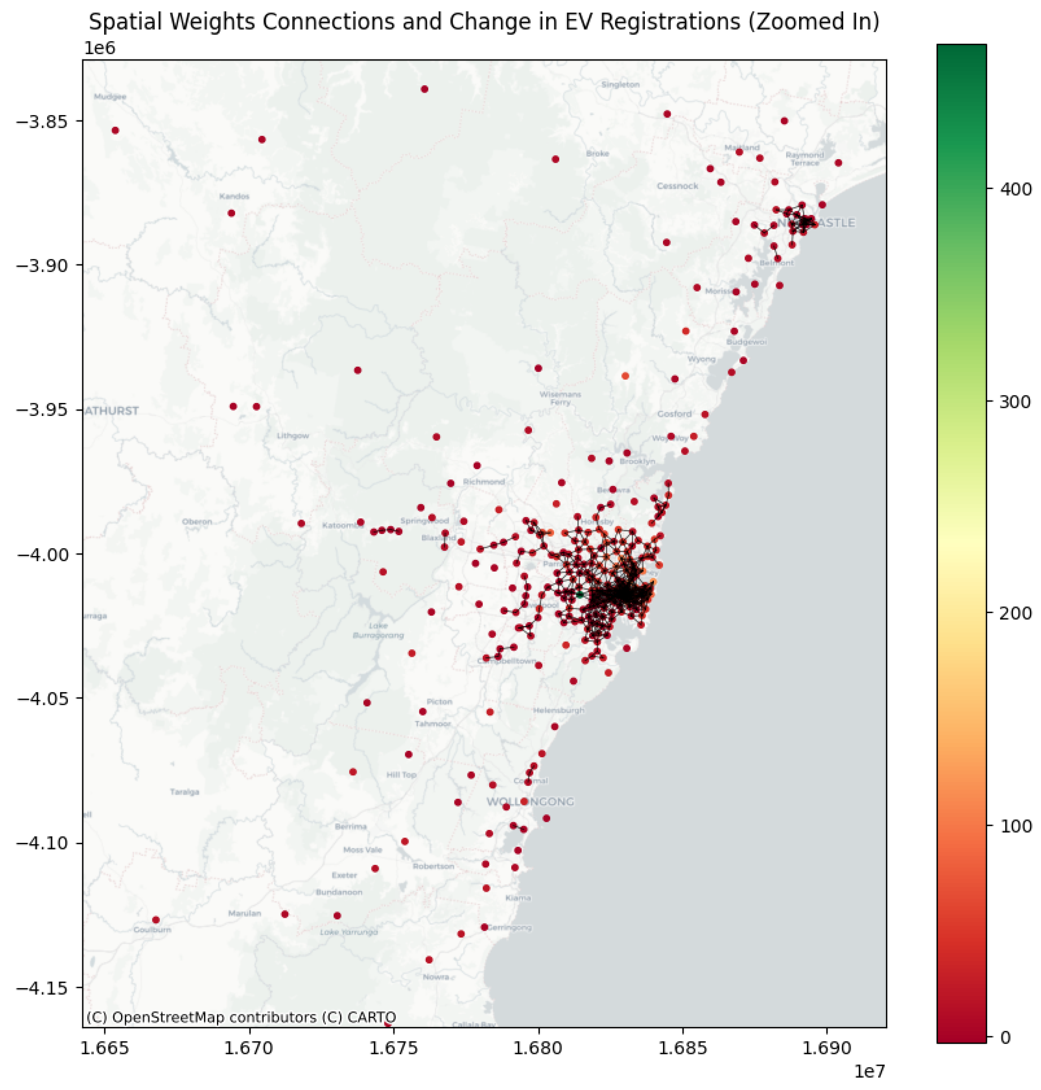
The spatial distribution of EV registrations across NSW demonstrates distinct geographic clustering, as illustrated in Figure 3. At the state level (Figure 4), three primary adoption zones emerge: Greater Sydney, which accounts for approximately 85% of all registrations; the Newcastle-Lake Macquarie region; and northern coastal areas around Byron Bay. This pattern reflects the concentration of both population density and economic affluence in these urban centers, with minimal uptake evident in regional and rural inland areas. The stark contrast between coastal urban regions and inland areas underscores the geographic inequality in EV access and adoption.
Within the Sydney metropolitan area (Figure 4), EV adoption exhibits pronounced intra-urban inequality. The eastern suburbs including Vaucluse, Bondi, and Dover Heights along with the Lower North Shore areas of Mosman and Lane Cove display the highest registration densities, corresponding precisely with the top-ranked postcodes identified in Table 2. These areas are characterized by high median incomes, high property values, and established affluence. Conversely, western and southwestern Sydney exhibit substantially lower adoption rates, appearing as lighter shaded areas on the map. This spatial divide highlights a socio-economic gradient that aligns closely with income and wealth distribution across the metropolitan area, with affluent eastern and northern suburbs demonstrating significantly higher EV uptake compared to lower-income western regions.
Despite a 417% increase in total EV registrations between 2017 and 2021, this fundamental spatial pattern remained remarkably stable over the period. Rather than diffusing uniformly across the metropolitan area, adoption expanded outward incrementally from the established affluent cores. This persistence suggests the presence of structural barriers to equitable EV access, including economic constraints, differential access to charging infrastructure, and socio-cultural factors that vary systematically across geographic space. The spatial concentration observed here motivates the regression analysis that follows, which seeks to quantify the specific socio-economic and demographic factors associated with these geographic disparities in EV adoption.
These descriptive statistics and spatial patterns establish the empirical context for understanding EV adoption in NSW. The substantial variation in both EV registrations and socio-economic characteristics across postcodes, combined with the clear geographic clustering of adoption, provides a strong foundation for regression analysis to identify the key drivers of early EV uptake.
3.3. Model Development and Refinement
It’s important to note that the independent variables have been standardised, which means that the coefficient of the variables represent a change in EV registrations for every one standard deviation increase, rather than a one-unit increase. The coefficients directly indicate the relative strength of the independent variables’ impacts on EV registration, with higher absolute values of coefficients suggesting a stronger correlation with EV registrations. Because of this standardisation, this leaves the intercept or constant term in the regression model irrelevant, as it represents the expected value of EV registrations when all the standardised independent variables are at their mean. The statistical significance of the model, however, remains unchanged, with the p values and standard errors being unaffected by this alteration of independent variables, and thus testing the statistical significance of the indicators to determining EV registrations [30].
Table 3 provides the initial model’s performance, highlighting the input independent variables, with their corresponding significance value, and the overall significance of the model itself. The adjusted R-squared value of 0.62 and R-squared value of 0.63 indicate that approximately 63% of the variance in EV registration data was explained by this model, suggesting a moderate to strong fit. The F-statistic of approx. 0 shows the model is statistically significant. The condition number of 8.83 also indicates that the model as a whole has little multicollinearity, based on this metric. Upon inspection of Table 3, however, with the threshold for multicollinearity being a value of 5, we can see several indicators being of concern, including proportion of car drivers, average weekly mortgage, proportion with no health condition and average income. Interpretation of these results in Table 3 thus has to be taken with precaution, as some variables that may initially seem to be insignificant may be skewed by this multicollinearity between variables. The key indicators that play into consideration here are the income and economic indicators, including average income, showing a p-value < 0.001 and a coefficient of 6.4167, meaning for every standard deviation increase in average income ($340.63), when all other variables are held constant, EV registration total count for a postcode is expected to rise by 6.4167, hence showing a positive association. A high proportion of manager and professional occupations also shows be positive association with EV registrations, with a p-value < 0.001, and a coefficient of 2.8479. This shows that areas with higher earning positions are more likely to adopt EVs. The other key indicator shown from this model is simply the number of households with vehicles, or in other words, the density of the postcode. With a p-value < 0.001, and a coefficient of 5.5682, this indicates that areas with a higher vehicle-owning population density are also a key indicator for which areas are adopting. An increase in the proportion of people aged 35-44 also showed a statistically significant negative association with the number of EV registrations, as such a lower proportion of people in this age range increases the estimated EV registrations, which didn’t align with my hypothesis of young adults with higher income than younger generations but being more environmentally conscious than older generations, would be higher adopters. Interestingly, an increase in average age for a postcode showed to be less statistically significant than the negatively associated proportion of people.
Some surprising results from this initial model showed that the average number of vehicles owned per household does not have a statistically significant association with EV registrations (in this model), with a t-statistic of -0.247. This could possibly be due to the high number of vehicles in regional areas. To combat this, the indicator was further investigated with compound effects on income and occupation; however, it still did not show statistical significance for the model. The proportion of car drivers for a postcode notably didn’t have a statistical impact, again, this was further investigated through the use of compound variables, however no statistical significance was found. Higher proportions of active transport, car drivers, marital status and non-religious showed to be insignificant to his model.
Critically, however, the residuals in this model are heavily right skewed, showing a skew of 3.8 and a kurtosis score of 36.327. Additionally, the JB p value is zero and as such indicating a non-normal distribution of residuals. This strongly suggests the residuals not normally distributed and thus the inference of the p values discussed is insignificant. To combat this, a logarithmic transformation was applied to the dependent variable, with the results shown in Table 4.
This model shows a dramatic improvement from the previous in many respects. Starting off with the R-squared value, this has increased by 20% from 0.63 to 0.827 and the F-statistic has risen from 67.46 to 189.6. This shows the log transformation dramatically improved the models explanatory power. Inspecting the residual indicators, it can be seen that the JB test statistic dropped dramatically from 29763 to 1.243 with a p-value of 0.527. Skewness improved from 3.821 to 0.022 (much closer to 0). Kurtosis improved from 36.327 to 3.216, which is very close to a normal distribution value of 3. The combination of these indicators shows that the log transformation successfully normalised the residuals and, as a result, increases the validity of the interpretation of independent variable coefficients and their statistical significance. Some notable changes in variable significance due to this transformation should be highlighted; average weekly mortgage p-value decreased from 0.164 to 0.000; proportion of people aged 35-44 p-value dramatically increased from 0.007 to 0.932; proportion of manager and professionals p-value increased from 0.000 to 0.081; and, proportion of people in service sector p-value decreased from 0.057 to 0.000. It can be seen how improper handling of residuals can lead to the dismissal and acceptance of statistically significant variables.
Table 5.
Initial Model Variance Inflation Factors (VIF) for Independent Variables.
| Variable | VIF |
|---|---|
| prop_car_driver | 7.1362 |
| avg_weekly_mortgage | 6.0203 |
| prop_no_health_cond | 5.9280 |
| avg_income | 5.8153 |
| prop_managers_professionals | 4.9603 |
| mean_mvs_per_dwelling | 4.9402 |
| apartment_proprtn | 4.2475 |
| currently_in_education_20plus_% | 4.1875 |
| avg_age_21 | 4.1631 |
| prop_age_35_44 | 3.7902 |
| prop_registered_marriage | 3.0536 |
| prop_service_sector | 2.1702 |
| prop_no_religion | 1.8775 |
| prop_active_transport | 1.8519 |
| households_with_cars | 1.4901 |
With this transformation however, it is again important to note the new method of interpreting the coefficients from the results, as the combination of the standardization of independent variables and the log transformation of dependent has an interesting effect. In essence, this combination means for low coefficients (< 0.1), the value represents the impact the independent variable has on the dependent as a percentage for a one unit increase of standard deviation when every other variable is held constant. When the coefficient is > 0.1 however, a transformation of must be applied. For example, from reading Table 4, households with cars has a coefficient of 0.5657, and as such, , meaning for every standard deviation increase in this variable, EV registrations increases by 76%. Alternatively, for low coefficients, the value can be directly interpreted. This now accounts and indicates that EV registrations do not increase linearly, with varying socio-economic and demographic factors. The following explains how this interpretation is allowed:
3.4. Final Model Results
Table 6 in the appendix section outlines only the statistically significant variables (8 in total) that contributed to the highest coefficient of determination (R-squared) value, and all variables having low multicollinearity. Overall, the model achieved an R-squared value of 0.819, showing a 19% increase from the initial model, and as such suggesting that 81.9% of the variance in EV registrations across the postcodes within NSW for 2021 could be explained by the selected socio-economic and demographic variables. Furthermore, the F-statistic of 339.4 and a p-value ≈ 0 confirm that the model as a whole is statistically significant. All the predictor variables shown in this Table 6 are statistically significant, being < 0.05, with the strongest predictor being the summation of income and mortgage together, having a coefficient of 0.7018 and hence positive association with EV registration count, taking a or 101.7% increase in registrations for every SD increase in both income and mortgage predictors. During development, a high collinearity between income and mortgage was discovered, and hence these two were joined together to reduce overall multicollinearity in the model. The second biggest influence in the model was the count of households with vehicles, which is essentially a proxy for the vehicle-owning population density of that suburb. This had a positive coefficient of 0.5928 and the highest t-statistic due to its minimal errors of 23.256, showing high statistical significance. This coefficient equates to a 80.9% increase in EV registrations for every SD increase in this households with vehicles count. Other key observations from the results show that demographic variables including average age ( = 0.0700, p = 0.032) and the proportion of managers and professionals ( = 0.0988, p = 0.023) showed modest positive associations. Educational engagement, measured through the percentage of those aged 20 and above currently in education ( = 0.0682, p = 0.042), demonstrated a similar positive relationship. The proportion of people reporting no religion ( = 0.0754, p = 0.004) and the proportion employed in the service sector ( = 0.1846, p < 0.001) both showed positive associations with EV registrations. Interestingly, the only negative relationship was observed with the proportion of active transport users ( = -0.0662, p = 0.005), suggesting that areas where people’s primary mode of transport to work is walking, running or cycling generally associated with a decrease in EV registrations.
The diagnostic tests conducted as shown in Table 5 in the appendix section, indicated no significant issues with the model assumptions. The Durbin-Watson statistic (1.710) suggested no concerning autocorrelation, while the Jarque-Bera test (JB = 0.021, p = 0.990) indicated the normality of residuals. The VIF tests (Table 7) revealed no severe multicollinearity, with all VIF values below 4, ranging from 1.15 to 3.85. The correlation matrix in Figure 5 shows that the highest correlations between independent variables were observed between income/mortgage status and the proportion of managers/professionals (r = 0.75), and between education status and average age (r = -0.52). These correlations indicate, unsurprisingly, that areas with higher proportions of managers and professionals tend to have higher income/mortgage status and that areas with higher proportions of students older than 20 tend to have a lower average age. None of the correlations however are strong enough to be of concern about multicollinearity, as such, these diagnostics collectively suggest that the model meets key OLS assumptions and can be considered reliable for statistical inference, thus completing the model validation.
3.5. Policy Implications
The clear correlation between higher income levels and EV registrations suggests the need for economic incentives to bridge the gap for individuals where income poses a significant barrier to EV adoption. Similar to successful models in Norway [31], income-based or means-tests subsidies could prove to be highly beneficial for democratising EV accessibility to low income households. By targeting incentives such as these, it would help reduce socio-economic disparities in EV ownership and as such facilitating a broader equitable adoption across NSW. Research by [32] supports the importance of such subsidies in bridging socio-economic gaps. Additionally, the findings in this research on a negative correlation between active transport use and EV registrations indicate that policy implementation may need to take a different approach in urban vs rural areas. In urban areas where active and public transport options are in abundance, policymakers may want to take into consideration the possibility of a hybrid policy, one which supports public and active transport use, as well as EV adoption, such a policy could provide rebates to EV owners for every kilometre travelled (calculated using opal), for example, may be useful in areas where EVs compliment current modes of transport. Furthermore, socio-cultural factors like non-religious affiliation as shown to be positively associated with EV registrations, add to this urban-rural divide and further encourage different policy or incentive strategies. To address this divide, communication techniques and language will need to be adjusted such that they resonate with the normalities of the local area culture, with the goal to emphasise practical benefits like cost savings and community health improvements. Additionally, this suggests a need to ensure that EV policies do not inadvertently widen socio-cultural divides, as outlined in previous studies examining similar disparities in renewable energy adoption.
Due to the strong positive association between vehicle ownership density and EV registrations, expanding charging infrastructure in urban areas can help further increase registration rates. The research conducted alludes to the fact that urban high-density areas may benefit from more accessible charging infrastructure, and is critical in areas where private parking is limited. Research by Hardman et al. (2018) highlights the importance of public charging infrastructure in increasing EV adoption in such areas. The focus on this infrastructure development could be on public spaces and multi-dwelling units, promoting registration in densely populated areas where EV ownership is feasible despite limited private charging options. Furthermore, through tentative use, this model may be used to forecast EV adoption, where the demand for charging infrastructure can be estimated, and as such local areas can be better prepared for an inevitable increased demand for such a network. Jung et al. [33] discuss the benefits of demand forecasting for infrastructure development, emphasizing how it can optimize resource allocation and improve user satisfaction with charging networks.
These findings also highlight the role of EV adoption as a tool for achieving NSW’s environmental objectives, such as those outlined in the NSW Electric Vehicle Strategy and national net-zero commitments. The alignment between higher EV adoption rates and local council areas with environmental goals supports the view that EV promotion can be integrated into broader net-zero strategies. Studies like McKinsey & Company [34] have highlighted the synergy between EV adoption and renewable energy goals, suggesting that an integrated approach could be beneficial in achieving NSW’s environmental targets. This would, however, require multi-level government support to create incentives that extend beyond vehicle subsidies to encompass renewable energy integration as well as EVs.
3.6. Limitations
It’s important to note the several limitations of these findings and how the results should be considered with precaution. Although the model used incorporates various significant variables like income, mortgage, vehicle density etc, it may overlook other influential factors that are harder to capture from ABS Census data such as environmental attitudes or access to renewable sources of energy, which have been linked to EV adoption. Due to the limited regional scope of this study being NSW, however, this means that incentive differences do not play into varying uptake across postcodes, thus keeping as a constant across all regions. Omitted variable bias may play a role, as without incorporating factors like attitude towards sustainability or technological literacy, the model may be significantly different. Additionally, the socio-economic variables collected are primarily focused around capturing the variability between regions in urban and surrounding areas, factors such as range anxiety or poor charging infrastructure that regional areas face may not be correctly captured by the indicators used in the outlined model. Limitations may also be present in the model’s predictive power for low uptake or non-suburban areas, as areas with higher adoption generally are biased by models such as these. As such, this limitation restricts its ability to predict EV adoption in lower-income regions or areas with limited infrastructure support, where adoption patterns may have a high variance. Furthermore, regression models are effective at establishing correlations between independent variables and a dependent, but this correlation does not equal causation, and as such, just because non-religious regions have been positively correlated with EV registrations, this does not mean that non-religious areas cause a positive increase in EV registrations. Finally, the regression model proposed in this research assumes that socio-economic indicators are relatively static, but these obviously fluctuate and change overtime, particularly in areas undergoing gentrification, and as such, using this model for forecasting purposes or for explaining shifts in adoption rates as regions evolve socio-economically may prove troublesome.
3.7. Discussion
After following the methodology approach outlined in this report, population density, high economic status, increased age, urban demographics and accessibility to EV charging all seem to have a positive association with an increase in EV registrations. To reiterate, the results showed that the strongest socio-economic variables, from those that were collected, were the combination of income and mortgage (representing areas of high economic status) and the amount of households that have vehicles, indicating the vehicle owning population density for the local area, showing expectedly that higher concentration population density is key to a high EV registration count. Each of these economic and demographic indicators respectively showed a 101.7% increase in EV registrations for every $493.46 increase in the combination of income and mortgage and a 80.9% increase in EV registrations for every 4664.75 increase in the count of households with cars, showing a strong positive association. These strong positive associations align with existing literature on EV adoption barriers. Numerous studies have identified purchase price as a primary barrier to EV adoption (Whitehead et al., 2019; Berkeley et al., 2017). The concentration of EV uptake in higher-income areas suggests that despite decreasing EV prices, financial constraints continue to influence adoption patterns. Additionally, the strong association outlined here aligns with a growing concern in the literature that EVs may be more accessible to affluent individuals, potentially encouraging socio-economic inequalities. In contrast, [35] noted that high-income groups are more likely to adopt EVs, driven by financial capability and environmental consciousness. All these insights suggest that income-based subsidies and incentives could help bridge the adoption gap for lower-income populations, supporting targeted policy interventions such as income-tested incentives or subsidies, as seen to be proven effective in Norway’s successful EV transition [31].
The service sector employment proportion, which had a coefficient of 0.1846, equating to a 20% increase in EV registration count for every 5.5% change, saw a positive relationship with EV adoption and may reflect the urban concentration of service jobs. Urban areas typically have more developed charging infrastructure and shorter average trip distances, factors previously identified as crucial for EV adoption [36]. Interestingly, the negative correlation with active transport, showing a coefficient of -0.0662 equating to a 6.8% decrease in EV registrations for every 5% increase in active transport, might indicate a complex relationship between urban density and EV adoption. Areas with high active transport usage often represent dense urban cores where private vehicle ownership, regardless of type, may be less necessary or practical, as such showing lower private vehicle ownership rates [37] . Furthermore, high urban areas have been previously linked to influence the availability of EV incentives, as governments in urban areas are more likely to support EV adoption as part of trying to meet environmental goals [38,39]. However, the complex interplay between urban areas and areas with increased active transport accessibility may make EV incentives less effective, as outlined here, so it is potentially important for EV incentives to be targeted in urban areas where active transport and even public transport accessibility is poor. The positive associations with educational engagement, which had a coefficient of 0.0682 equating to a 6.8% increase in EV registrations for every 3% increase in education engagement and age, which had a coefficient of 0.0700 equating to a 6.9% increase in EV registrations for every 4.22 increase in average age, suggest that EV adoption is higher in areas with educated, economically established populations. This aligns with Rogers’ diffusion of innovation theory Rogers [5], where early adopters tend to have higher educational levels and greater access to information [40]. This greater access to information can increase the awareness of the potential long term cost savings that come with EVs, as well as generating social ’hype’ around new technologies, creating a network bubble effect, influencing more people and gaining greater awareness in turn. This could indicate that targeted educational campaigns may further accelerate adoption, especially in areas with high levels of educational attainment. The positive relationship with non-religious affiliation, which had a coefficient of 0.0754, equating to a 7.8% increase in EV registrations for 11% increase of the independent, might reflect broader socio-cultural factors or urban-rural divides. These findings can suggest a broader cultural divide in EV adoption, potentially linked to an urban versus rural mindset or progressive versus conservative social views. Regions with higher proportions of non-religious individuals might indicate urban or progressive areas, which are generally more environmentally conscious and adopt new technologies [40]. This social and cultural distinction is supported by findings from [41], who noted that cultural attitudes towards sustainability are significant predictors of EV adoption, with pro-environmental attitudes more prevalent among non-religious or secular communities. More in-depth analysis would be required to understand the true effect of this non-religious influence however.
It’s important to note the variables that were deemed insignificant as well, as these can help to shed light onto what has been shown not to have a significant impact on EV registrations, and thus may allow for a more refined hypothesis or understanding of what are the general types of socio-economic and demographic indicators do have an influence. From the model highlighted in Table 3, the average number of motor vehicles (p-value of 0.211), proportion of apartments (p-value of 0.378), proportion of people that drive to work (p-value of 0.32) and proportion of registered marital status (p-value of 0.4310) all showed to have no significant relationship with EV adoption. The insignificance of motor vehicles per dwelling and apartment dwelling is somewhat surprising given previous literature. For instance, [42] found that having access to private parking and charging infrastructure (which is typically more challenging in apartments) was an important factor in EV adoption. However, our results suggest these physical infrastructure factors may be less important than previously thought, possibly due to improving public charging networks addressing these constraints. Studies like Sovacool et al. [8] emphasised how accessible public charging infrastructure can be a big factor in addressing limitations faced by apartment residents and potentially enhancing EV adoption in dense urban areas. The insignificance of car driver proportion and marriage status aligns better with expectations. While some studies have examined demographic factors in EV adoption [36,43,44], there is limited theoretical basis for why being a regular car driver or being married would specifically influence EV purchases. The lack of significance for these variables suggests that EV adoption is driven more by economic factors (as shown by the significance of income and mortgage variables) and social/attitudinal factors (as shown by education and professional status variables) rather than basic demographic characteristics.
4. Conclusions
As the race to mitigate the effects of climate change on our world continues, there is a global conscious responsibility now around cementing a sustainable future, and as such sustainable energy product and consumption goals are being set by nations worldwide. EV adoption has proven to be a crucial player to help reach these sustainability goals, drastically reducing greenhouse gas emissions through zero tailpipe emissions (although the energy production still needs to be conducted sustainably down the supply chain). As such, due to this, EV adoption has been on a steady rise since the early 2010s, with nearly a 10% market share of all new vehicle sales in NSW for Q3 of 2024. By analysing the socio-economic and demographic characteristics of the areas that are adopting these EVs, as done in this research, the hope is to gain a better understanding of the key factors that influence the population to adopt this technology, and what types of communities are adopting. By understanding this, better decisions can be made around marketing, education, policy-making and infrastructure planning, which in turn will increase EV market penetration and, as a whole, build consumer trust.
The results from this study, in the context of the model used in OLS regressional analysis, shows several factors to be of significance to an increase in EV registrations or adoption. The most significant with a positive association proved to be the population density of car owners, and the combination of income and mortgage payments (economic status), which heavily aligned with previous literature. Next, which also had a positive association with an increase in EV adoption, but to a lesser extent, were age, high-paying occupational roles, education, non-religious areas and areas with an increased service sector (increased urbanisation). Interestingly, areas with an increased proportion of active transportation use saw a negative association with EV adoption. Indicators that proved to be insignificant from this analysis included the average number of vehicles owned per dwelling, health, marital status and, interestingly, the general dwelling structure for an area.
As a result, these findings further support previous literature, highlighting the key role income and population density has to play on EV adoption. Furthermore, it also supports other previous literature stating that areas with higher education rates have a positive effect on adoption but interestingly, this study disagreed with older previous literature that stated increased apartment living shows a negative association with EV adoption. Thus potentially highlighting how an increase in charging infrastructure accessibility has reduced this negative association, indicating the positive impact of good infrastructure planning. As a recommendation, policy makers should further focus their efforts on bridging the economic gap for individuals where income is a significant barrier, implementing income-based or means-tested subsidies could prove to be greatly beneficial for increasing EV uptake, as shown by the strong association with income and EV uptake found in this study. As a result, these efforts would help the NSW state government to close the gap to their net-zero goal by 2030 and as a whole reduce greenhouse gas emissions.
As highlighted previously and due to the limitations of this research, an increased dataset for both the dependent variable (increased POA regions) and a greater granularity of the independent variable, including the addition of consumer behaviour indicators, environmental tendencies, and social status, could be valuable insights to improving the understanding of EV adoption. Building on from an increased dataset, future research could benefit from taking a longitudinal study approach. This would encapsulate the changing adoption rate of EVs over time, highlighting trends and the long-term impact of interventions such as policy making and infrastructure planning. In this longitudinal study, an interesting approach would be analysing how the introduction of policies and charging infrastructure have an affect on EV adoption. After determining the constant rate of increase of EV adoption for an area, accessing how this changes after EV charging stations and policies in the local government area have been introduced would indeed be informative about the actual impact and efficacy such policy and infrastructure planning has on EV adoption. Furthermore, this study would shed light on the importance of increasing charging infrastructure to help accelerate EV adoption rates in regional and rural areas, possibly being of great importance to strategic investments in EV support systems throughout NSW.
Author Contributions
Conceptualization, Kaveh Khalilpour; methodology, Lachlan J. Masters; data curation, Lachlan J. Masters; formal analysis, Lachlan J. Masters; validation, Lachlan J. Masters, Tallat Jabeen, and Mohammad Karimadini; writing-original draft preparation, Lachlan J. Masters, Tallat Jabeen, and Mohammad Karimadini; writing-review and editing, Marty Fuentes, Faezeh Karimi, and Kaveh Khalilpour; supervision, Kaveh Khalilpour. All authors have read and agreed to the published version of the manuscript.
Funding
This research received no external funding.
Institutional Review Board Statement
Not applicable.
Informed Consent Statement
Not applicable.
Data Availability Statement
All data is provided in the article.
Acknowledgments
Generative AI was used for language refinement, such as checking grammar and correcting typographical errors. The authors reviewed and edited the manuscript, and take full responsibility for the content of this publication.
Conflicts of Interest
The authors declare no conflicts of interest.
Abbreviations
The following abbreviations are used in this manuscript:
| UTS | University of Technology Sydney |
| EV | Electric Vehicle |
| ICE | Internal Combustion Engine |
| NSW | New South Wales |
| ABS | Australian Bureau of Statistics |
| POA | Postal Area |
| SA2 | Statistical Area Level 2 |
| DOI | Diffusion of Innovation Theory |
| VIF | Variance Inflation Factor |
| OLS | Ordinary Least Squares |
| SD | Standard Deviation |
Appendix A. Extended Results
Out of curiosity, a model was made with pure compounds, leading to the following results.
Table A1.
Finalised Model OLS Regression Results for EV Registrations in 2021.
| Variable | Coefficient | t-Statistic | P-value |
|---|---|---|---|
| Constant | 6.2677 | 16.735 | 0.000 |
| Households_with_Cars | 6.1487 | 18.713 | 0.000 |
| Income_Mortgage_Compound | 6.8888 | 16.640 | 0.000 |
| Cars_Income | 7.4584 | 17.502 | 0.000 |
| Cars_Age | 1.2005 | 3.389 | 0.001 |
| Income_Managers | 4.0493 | 11.794 | 0.000 |
| Transport_Education | 1.1088 | 4.063 | 0.000 |
| House_Professionals | 2.2749 | 7.152 | 0.000 |
| Model Summary | |||
| R-squared | 0.764 | ||
| Adj. R-squared | 0.761 | ||
| F-statistic | 278.9 | ||
| Prob (F-statistic) | 2.12e-184 |
Table A2.
Finalised Model Correlation Matrix of Independent Variables.
| 1 | 2 | 3 | 4 | 5 | 6 | 7 | |
|---|---|---|---|---|---|---|---|
| (1) Households w Cars | 1.00 | ||||||
| (2) Income Mortgage | 0.21 | 1.00 | |||||
| (3) Cars Income | -0.15 | -0.09 | 1.00 | ||||
| (4) Cars Age | -0.36 | 0.079 | -0.17 | 1.00 | |||
| (5) Income Managers | 0.063 | 0.68 | -0.019 | 0.089 | 1.00 | ||
| (6) Transport Education | 0.068 | 0.16 | -0.087 | -0.019 | 0.076 | 1.00 | |
| (7) House Professionals | -0.062 | -0.55 | -0.054 | -0.070 | -0.72 | -0.27 | 1.00 |
Table A3.
Finalised Model Variance Inflation Factors (VIF) for Independent Variables.
| Variable | VIF |
|---|---|
| Income_Managers | 3.08 |
| House_Professionals | 2.72 |
| Income_Mortgage_Compound | 1.84 |
| Cars_Age | 1.31 |
| Households_with_Cars | 1.31 |
| Cars_Income | 1.20 |
| Transport_Education | 1.15 |
The variable with the highest coefficient and thus the biggest impact on the model is Cars Income (), which is a compound variable of the amount of households with cars multiplied by the income mortgage compound. This had a coefficient of 7.46 and hence for every standard deviation increase of the compound variables, results in a registration increase of 7.46, showing areas with car ownership and financial capacity has a positive association with EV registrations. Next was the combination of average income per week and average mortgage repayment per week (), with a 6.89 increase in ev registrations for every standard deviation increase of the combination of income and mortgage, showing areas with higher combined income and mortgage repayments show a positive relationship to EV registration. Households with cars follows (), with a 6.15 increase in EV registration numbers for every standard deviation increase in households with cars (4664.75), as such higher car ownership in households is positively associated with increased EV registration. Following is the compound variable of income mortgage multiplied by the proportion of people that are in professional or managerial occupational roles (). The results show that for every standard deviation increase in these socio-economic variables, in conjunction with each other, produces a 4.05 increase in EV registration, and as such shows postcodes with a higher concentration of managers and professionals with higher income is positively associated with the dependent variable. The next most significant indicator was deemed to be the compound of the proportion of separate houses or dwellings multiplied by the proportion of people working in professional and managerial occupations (). Again, results show that for the compound increase in these variables leads to a 2.27 increase in EV registrations, indicating a positive association of the dependent variable with individuals who live in houses and working in professional or managerial occupations. Next was the compound of proportion of households with cars multiplied by average age, combining to describe the age of car owning populations, and the effect on EV registrations. This had a , and a coefficient of 1.20. Finally, the last indicator used in this model is the compound of proportion of active commuters to work and the proportion of students over 20, showing a positive association with an increase in EV registrations, thus describing areas of greater education and higher environmental awareness. This had the smallest impact on the model with a coefficient of 1.11 and a .
Upon inspection of the correlation matrix results (see Table A2), it can be seen that the highest correlation lies between the Income Managers compound and House Professionals compound, showing a negative correlation score of -0.72, as such suggesting difference in housing preferences among professionals based on income. The correlation between Income Mangers and Income is shown to be moderate positive with a score of 0.68, indicating postcodes with higher incomes tend to have more professionals and managers, which is to be expected. The Income and House Professionals compound showed a -0.55 correlation, suggesting an inverse relationship between higher income areas and the proportion of professionals living in separate houses. Overall however, although there are some interrelationships among the independent variables, the remain low with the highest being 0.72.
Inspecting the VIF results (see Table A3), shows a range of VIF values from 1.15 to 3.08, indicating low to moderate multicollinearity within the model. Being below the threshold value of 5 however, this suggests that multicollinearity does not pose a significant issue to the model. As such, this allows for the reliable interpretation of each variables independent contribution to the EV adoption model.
Appendix B. Spatial Analysis
The spatial analysis is illustrated in Figure A1.
Figure A1.
Spatial Analysis of Sydney (threshold=500).
References
- International Energy Agency. Global EV Outlook 2023, 2023. Retrieved from the International Energy Agency.
- United Nations Environment Programme. Emissions Gap Report 2021, 2021. Retrieved from UNEP.
- on Climate Change (IPCC), I.P. Global Warming of 1.5°C. An IPCC Special Report on the impacts of global warming of 1.5°C above pre-industrial levels and related global greenhouse gas emission pathways, in the context of strengthening the global response to the threat of climate change, sustainable development, and efforts to eradicate poverty, 2018.
- Association, A.A. Electric Vehicle Index, 2024.
- Rogers, E.M. Diffusion of Innovations, 5th ed.; Free Press: New York, 2003. [Google Scholar]
- Geoffrey, M.; Regis, M. Crossing the chasm: Marketing and selling high-tech products to mainstream customers. HarperBusiness Essentials 1991.
- Rogers, E.M.; Singhal, A.; Quinlan, M.M. Diffusion of innovations. In An integrated approach to communication theory and research; Routledge, 2014; pp. 432–448. [Google Scholar]
- Sovacool, B.K.; Axsen, J.; Kempton, W. The future promise of vehicle-to-grid (V2G) integration: a sociotechnical review and research agenda. Annual Review of Environment and Resources 2017, 42, 377–406. [Google Scholar] [CrossRef]
- Nikolova, B.; Mickwitz, P. Consumer Adoption of Electric Vehicles in Australia: Barriers and Policy Enablers. Transport Reviews 2019, 39, 310–332. [Google Scholar]
- Coffman, M.; Bernstein, P.; Wee, S. Electric Vehicles Revisited: A Review of Factors that Influence Adoption. Transport Reviews 2017, 37, 79–93. [Google Scholar] [CrossRef]
- Jenn, A.; Springel, K.; Gopal, A.R. Effectiveness of Electric Vehicle Incentives in the United States. Energy Policy 2018, 119, 349–356. [Google Scholar] [CrossRef]
- Hall, D.; Lutsey, N. Electric Vehicle Charging Infrastructure: Guidelines for Cities. The International Council on Clean Transportation, 2019.
- Nicholas, M.; Hall, D. Lessons Learned on Early Electric Vehicle Fast-Charging Deployments. The International Council on Clean Transportation, 2018.
- Rohdin, P.; Thollander, P.; Solding, P. Barriers to and Drivers for Energy Efficiency in the Swedish Industry. Energy 2020, 35, 2318–2324. [Google Scholar] [CrossRef]
- Mortimore, A.; Ratnasiri, S.; Iftekhar, M.S. Who is buying electric vehicles in Australia? A study of early adopters. Australasian Journal of Environmental Management 2024, 31, 136–160. [Google Scholar] [CrossRef]
- Consumer Policy Research Centre (CPRC). The Barriers and Potential Enablers of Electric Vehicle Uptake in Australia. CPRC Working Paper, 2022.
- Anakpo, G.; Oyenubi, A. Technological innovation and economic growth in Southern Africa: Application of panel dynamic OLS regression. Development Southern Africa 2022, 39, 543–557. [Google Scholar] [CrossRef]
- Hussain, S.; Maqbool, R.; Hussain, A.; Ashfaq, S. Assessing the Socio-Economic Impacts of Rural Infrastructure Projects on Community Development. Buildings 2022. [Google Scholar] [CrossRef]
- Rungskunroch, P.; Shen, Z.J.; Kaewunruen, S. Benchmarking Socio-Economic Impacts of High-Speed Rail Networks Using K-Nearest Neighbour and Pearson’s Correlation Coefficient Techniques through Computational Model-Based Analysis. Applied Sciences 2022. [Google Scholar] [CrossRef]
- Certo, S.T.; Raney, K.A.; Albader, L.; Busenbark, J.R. Out of Shape: The Implications of (Extremely) Nonnormal Dependent Variables. Organizational Research Methods 2023, 27, 195–222. [Google Scholar] [CrossRef]
- Darda, M.A.; Bhuiyan, M.A.H. A Structural Equation Model (SEM) for the socio-economic impacts of ecotourism development in Malaysia. PLoS ONE 2022, 17. [Google Scholar] [CrossRef]
- Birol, E.; Bouis, H. Role of socio-economic research in developing, delivering and scaling new crop varieties: the case of staple crop biofortification. Frontiers in Plant Science 2023, 14. [Google Scholar] [CrossRef] [PubMed]
- Xia, Z.; Wu, D.; Zhang, L. Economic, Functional, and Social Factors Influencing Electric Vehicles’ Adoption: An Empirical Study Based on the Diffusion of Innovation Theory. Sustainability 2022, 14, 6283. [Google Scholar] [CrossRef]
- Harrell Jr, F.E. Ordinal logistic regression. In Regression modeling strategies: with applications to linear models, logistic and ordinal regression, and survival analysis; Springer, 2015; pp. 311–325. [Google Scholar]
- Mapping, E.I. Chargers by Postcode Prototype Dataset, 2024.
- of Statistics (ABS), A.B. Australian Statistical Geography Standard (ASGS): Edition 3, July 2021 – June 2026, Allocation Files, 2021.
- Proctor, M. Australian Postcodes Dataset, 2024.
- Yang, M.; Gao, X. Log-Linear Models Have Been Widely Used in Modeling Consumer Choice, Income Distribution, and Market Demand: Foundations, Recent Developments, and a Practical Guide. Journal of Choice Modelling 2019, 32, 100–171. [Google Scholar]
- Office of the Australian Information Commissioner. Australian Privacy Principles, 1988. Accessed: 2024-11-10.
- Bring, J. How to Standardize Regression Coefficients. The American Statistician 1994, 48, 209–213. [Google Scholar] [CrossRef]
- Figenbaum, E. Norway—The world leader in BEV adoption. In Who’s driving electric cars: Understanding consumer adoption and use of plug-in electric cars; Springer, 2020; pp. 89–120. [Google Scholar]
- Li, J.; Chew, A.; Wang, H. Investigating state-of-the-art planning strategies for electric vehicle charging infrastructures in coupled transport and power networks: A comprehensive review. Progress in Energy 2024. [Google Scholar] [CrossRef]
- Jung, F.; Schröder, M.; Timme, M. Exponential adoption of battery electric cars. PLoS one 2023, 18, e0295692. [Google Scholar] [CrossRef] [PubMed]
- McKinsey & Company. Scaling EV infrastructure to meet net-zero targets. https://www.mckinsey.com/industries/electric-power-and-natural-gas/our-insights/voices-on-infrastructure-scaling-ev-infrastructure-to-meet-net-zero-targets, 2021. Accessed: 2025-12-22.
- Chandra, M. Investigating the impact of policies, socio-demography and national commitments on electric-vehicle demand: Cross-country study. Journal of Transport Geography 2022, 103, 103410. [Google Scholar] [CrossRef]
- Hardman, S.; Jenn, A.; Tal, G.; Axsen, J.; Beard, G.; Daina, N.; Figenbaum, E.; Jakobsson, N.; Jochem, P.; Kinnear, N.; et al. A review of consumer preferences of and interactions with electric vehicle charging infrastructure. Transportation Research Part D: Transport and Environment 2018, 62, 508–523. [Google Scholar] [CrossRef]
- Ashik, F.R.; Rahman, M.H.; Zafri, N.M.; Antipova, A.; Labib, S. Car ownership, commute distance, and commute mode choice in the dense megacity of a developing country: The direct and indirect role of the built environment. Transportation Research Record 2024, 2678, 1923–1938. [Google Scholar] [CrossRef]
- Langbroek, J.H.; Franklin, J.P.; Susilo, Y.O. The effect of policy incentives on electric vehicle adoption. Energy Policy 2016, 94, 94–103. [Google Scholar] [CrossRef]
- Kohn, E.; Huang, C.; Kong, N.; Hardman, S. Electric Vehicle Incentives in 15 Leading Electric Vehicle Markets. Technical report, Plug-in Hybrid & Electric Vehicle Research Center, Institute of Transportation Studies, University of California, Davis, 2022. Accessed: 2025-12-23.
- Yadav, R.; Radha Yadav author = Rambalak Yadav and Radha Yadav, k.E. Are consumers ready to adopt electric vehicles? Analyzing the barriers and motivators associated with electric vehicle adoption in India: Policy implications for various stakeholders. Energy Policy 2024, 190, 114173. [Google Scholar] [CrossRef]
- Tang, M.; Cao, J.; Fan, Z.; Gong, D.; Xue, G. Public Perceptions of EV Charging Infrastructure: A Combined Sentiment Analysis and Topic Modeling Approach. Studies in Informatics and Control 2024, 33, 59–72. [Google Scholar] [CrossRef]
- Peters, A.; Dütschke, E. How do Consumers Perceive Electric Vehicles? A Comparison of German Consumer Groups. Journal of Environmental Policy & Planning 2014, 16. [Google Scholar] [CrossRef]
- Egbue, O.; Long, S. Barriers to widespread adoption of electric vehicles: An analysis of consumer attitudes and perceptions. Energy policy 2012, 48, 717–729. [Google Scholar] [CrossRef]
- Pandita, D.; Bhatt, V.; Kumar, V.R.; Fatma, A.; Vapiwala, F. Electrifying the future: analysing the determinants of electric vehicle adoption. International Journal of Energy Sector Management 2024, 18, 1767–1786. [Google Scholar] [CrossRef]
Figure 1.
Conceptual overview of the study context, illustrating the socio-economic and demographic drivers of electric vehicle adoption in New South Wales, the data sources employed, the analytical approach, and the policy-relevant outcomes considered.
Figure 1.
Conceptual overview of the study context, illustrating the socio-economic and demographic drivers of electric vehicle adoption in New South Wales, the data sources employed, the analytical approach, and the policy-relevant outcomes considered.
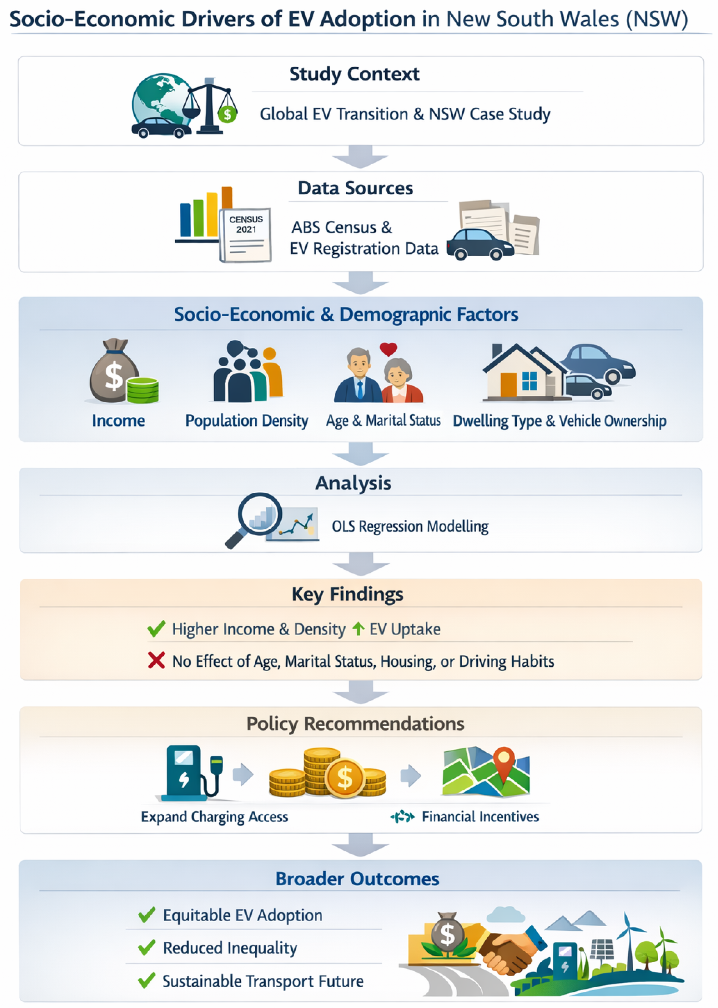
Figure 2.
Analysis Methodology Flow Chart.
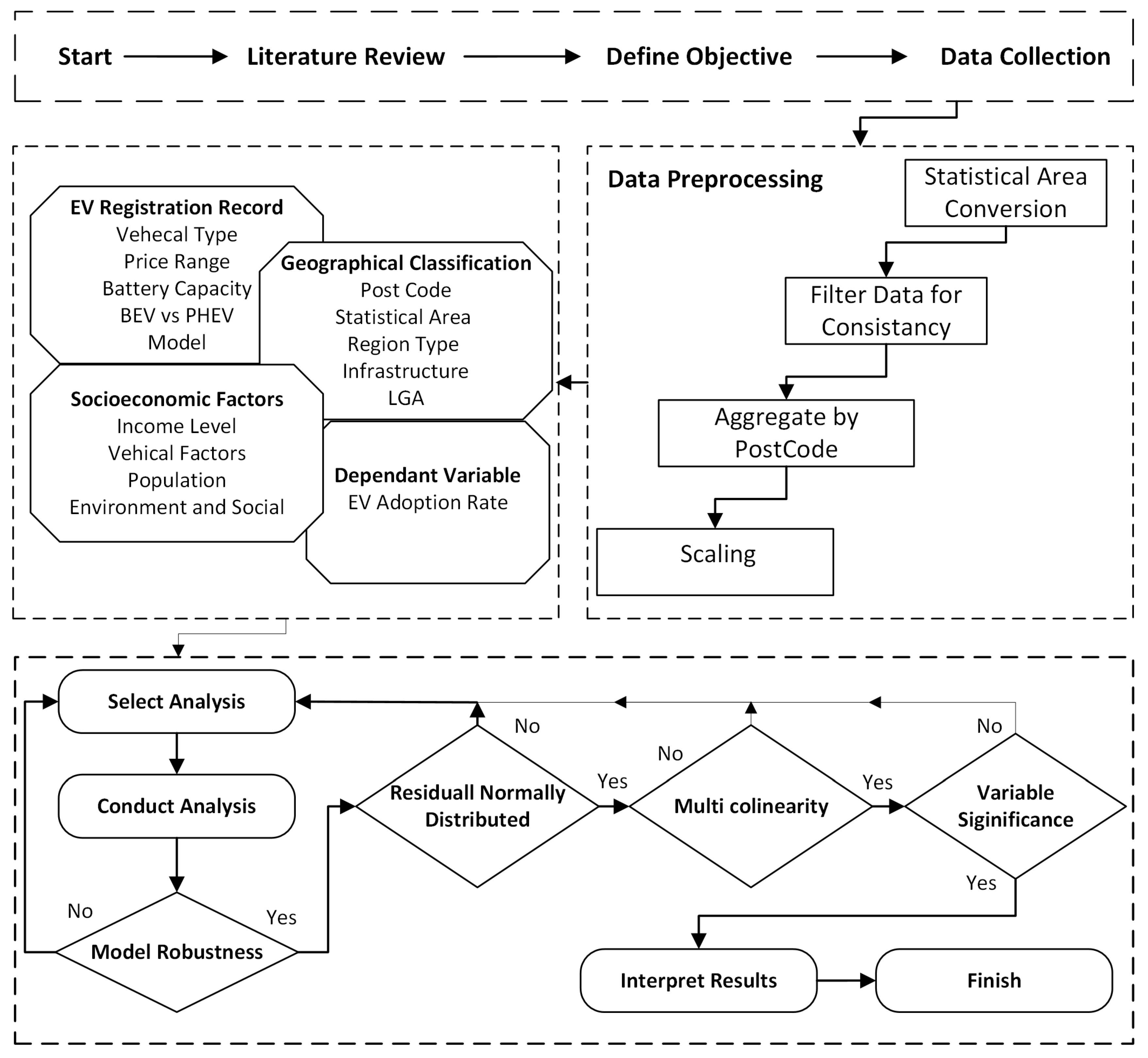
Figure 3.
NSW Heatmap of Registrations 2021.
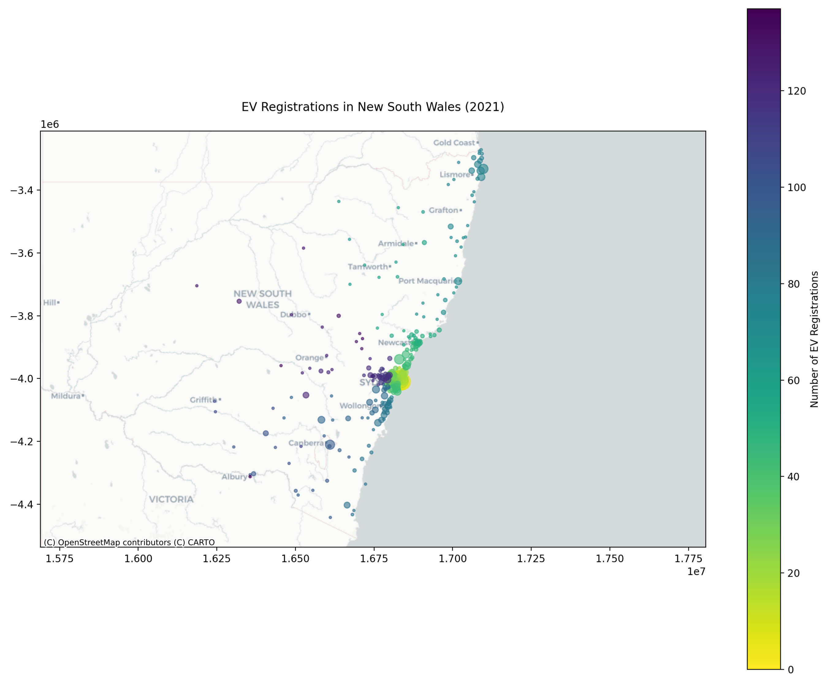
Figure 4.
Sydney Heatmap Registrations 2021.
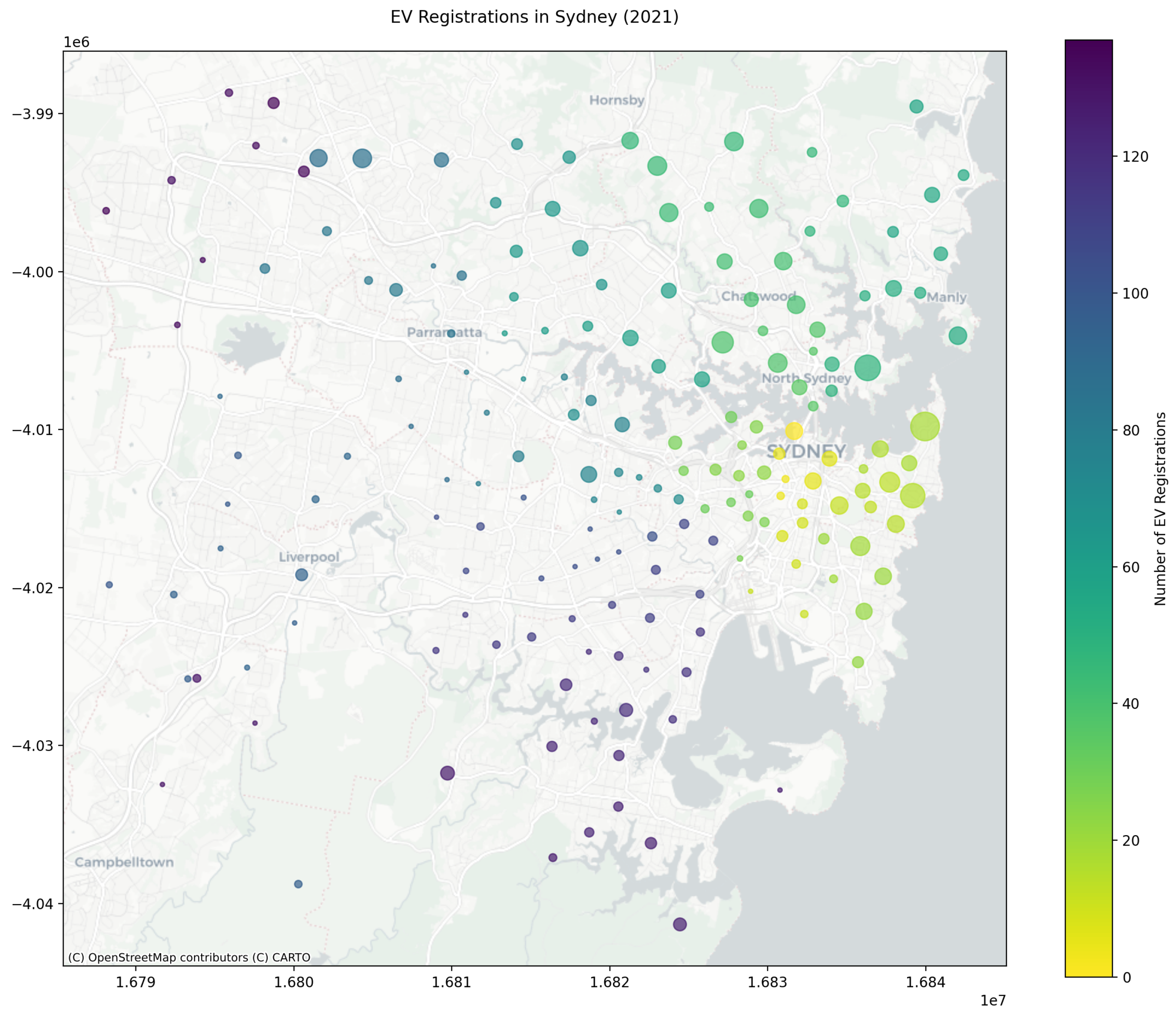
Figure 5.
Final Model Correlation Matrix.
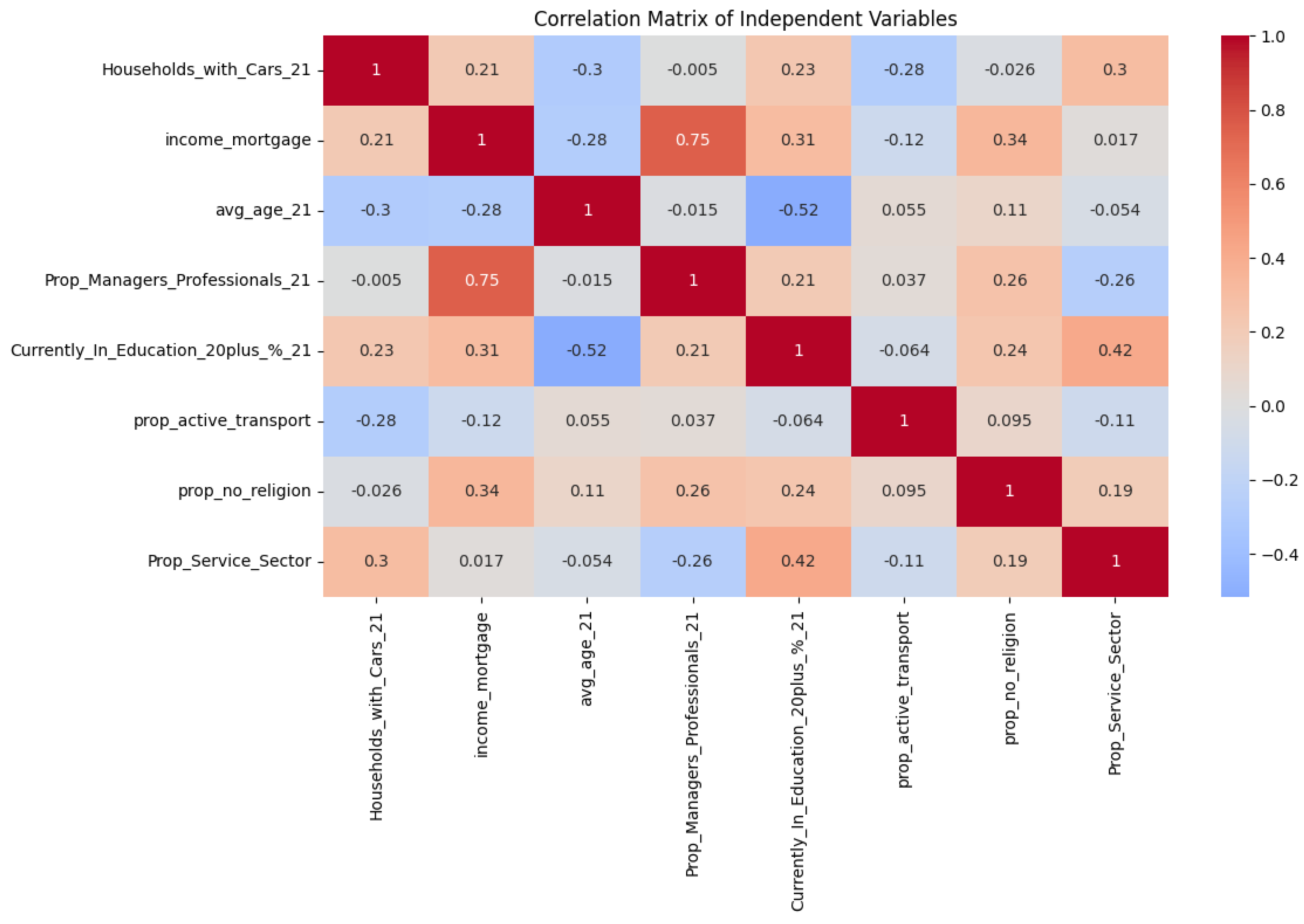
Table 1.
Summary Statistics of Key Variables in EV Uptake Study Dataset.
| Variable | Type | Mean | Std Dev | Min | Max |
|---|---|---|---|---|---|
| Postcode | int64 | 2423.88 | 262.08 | 2000.00 | 2898.00 |
| Latitude | float64 | −33.19 | 1.77 | −37.27 | −28.18 |
| Longitude | float64 | 150.29 | 2.06 | 141.80 | 159.08 |
| EV Registrations | float64 | 9.27 | 14.55 | 0.00 | 137.00 |
| Mean MVs per Dwelling | float64 | 1.80 | 0.34 | 0.53 | 2.66 |
| Households with Cars | float64 | 4252.06 | 4664.75 | 0.00 | 31624.00 |
| Avg Income ($) | float64 | 1104.80 | 340.63 | 306.93 | 2301.35 |
| Avg Weekly Mortgage ($) | float64 | 495.82 | 152.83 | 86.54 | 867.73 |
| Avg Weekly Rent ($) | float64 | 311.05 | 96.26 | 37.50 | 537.23 |
| Avg Age (years) | float64 | 40.28 | 4.22 | 19.93 | 55.51 |
| Prop Apartment (%) | float64 | 9.97 | 19.11 | 0.00 | 99.25 |
| Prop House (%) | float64 | 82.68 | 25.08 | 0.00 | 117.86 |
| Prop Public Transport | float64 | 0.02 | 0.02 | 0.00 | 0.15 |
| Prop Active Transport | float64 | 0.04 | 0.05 | 0.00 | 0.74 |
| Prop Car Driver | float64 | 0.48 | 0.16 | 0.07 | 0.73 |
| Prop Registered Marriage | float64 | 0.47 | 0.08 | 0.00 | 1.00 |
| Prop No Religion | float64 | 0.34 | 0.11 | 0.07 | 0.67 |
| Prop No Health Condition | float64 | 0.61 | 0.08 | 0.38 | 0.87 |
| Prop Service Sector | float64 | 18.14 | 5.31 | 0.00 | 57.61 |
Table 3.
Initial Model OLS Regression Results for EV Registrations in 2021 (Standardisation of Independent Variables).
Table 3.
Initial Model OLS Regression Results for EV Registrations in 2021 (Standardisation of Independent Variables).
| Variable | Coefficient | t-Statistic | P-value |
|---|---|---|---|
| const | 9.2684 | 25.559 | 0.000 |
| mean_mvs_per_dwelling | -0.1993 | -0.247 | 0.805 |
| households_with_Cars | 5.5682 | 12.579 | 0.000 |
| avg_income | 6.4167 | 7.338 | 0.000 |
| avg_weekly_mortgage | 1.2410 | 1.395 | 0.164 |
| avg_age | 0.5146 | 0.695 | 0.487 |
| proportion_age_35_44 | -1.9104 | -2.706 | 0.007 |
| prop_managers_professionals | 2.8479 | 3.526 | 0.000 |
| currently_in_education_20plus_% | -0.4957 | -0.668 | 0.504 |
| apartment_proprtn | 0.5425 | 0.726 | 0.468 |
| prop_active_transport | 0.2150 | 0.436 | 0.663 |
| prop_car_driver | -0.0927 | -0.096 | 0.924 |
| prop_registered_marriage | 0.1904 | 0.300 | 0.764 |
| prop_no_religion | -0.1709 | -0.344 | 0.731 |
| prop_no_health_cond | 0.8446 | 0.957 | 0.339 |
| prop_service_sector | 1.0196 | 1.909 | 0.057 |
| Model Summary | |||
| R-squared | 0.630 | ||
| Adj. R-squared | 0.620 | ||
| F-statistic | 67.46 | ||
| Prob (F-statistic) | 1.52e-117 | ||
| Residual Diagnostics | |||
| Skew | 3.821 | ||
| Kurtosis | 36.327 | ||
| JB test | 0.00 | ||
| Durbin-Watson | 1.641 |
Table 4.
Initial Model OLS Regression Results for EV Registrations in 2021 (Logarithmic Dependent Variable Transformation + Standardisation of Independent Variables).
Table 4.
Initial Model OLS Regression Results for EV Registrations in 2021 (Logarithmic Dependent Variable Transformation + Standardisation of Independent Variables).
| Variable | Coefficient | t-Statistic | P-value |
|---|---|---|---|
| Constant | 1.5544 | 71.431 | 0.000 |
| Mean_MVs_per_dwelling | -0.0606 | -1.253 | 0.211 |
| Households_with_Cars | 0.5657 | 21.298 | 0.000 |
| Avg_Income | 0.3583 | 6.828 | 0.000 |
| avg_weekly_mortgage | 0.3302 | 6.184 | 0.000 |
| avg_age | 0.1054 | 2.375 | 0.018 |
| proportion_age_35_44 | 0.0036 | 0.086 | 0.932 |
| Prop_Managers_Professionals | 0.0847 | 1.748 | 0.081 |
| Currently_In_Education_20plus_% | 0.0197 | 0.442 | 0.658 |
| apartment_proprtn | -0.0396 | -0.882 | 0.378 |
| prop_active_transport | -0.0770 | -2.601 | 0.010 |
| prop_car_driver | -0.0579 | -0.996 | 0.320 |
| prop_registered_marriage | -0.0300 | -0.788 | 0.431 |
| prop_no_religion | 0.0941 | 3.155 | 0.002 |
| Prop_No_Health_Cond | 0.0773 | 1.459 | 0.145 |
| Prop_Service_Sector | 0.1519 | 4.740 | 0.000 |
| Model Summary | |||
| R-squared | 0.827 | ||
| Adj. R-squared | 0.823 | ||
| F-statistic | 189.6 | ||
| Prob (F-statistic) | 4.58e-215 | ||
| Residual Diagnostics | |||
| Skew | 0.022 | ||
| Kurtosis | 3.216 | ||
| JB test | 0.537 | ||
| Durbin-Watson | 1.767 |
Table 6.
Final Model OLS Regression Results for EV Registrations in 2021 (Logarithmic Dependent Variable Transformation + Standardisation of Independent Variables).
Table 6.
Final Model OLS Regression Results for EV Registrations in 2021 (Logarithmic Dependent Variable Transformation + Standardisation of Independent Variables).
| Variable | Coefficient | t-Statistic | P-value |
|---|---|---|---|
| Constant | 1.5544 | 70.163 | 0.000 |
| Households_with_Cars | 0.5928 | 23.256 | 0.000 |
| income_mortgage | 0.7018 | 16.281 | 0.000 |
| avg_age | 0.0700 | 2.154 | 0.032 |
| Prop_Managers_Professionals | 0.0988 | 2.271 | 0.023 |
| Currently_In_Education_20plus | 0.0682 | 2.035 | 0.042 |
| prop_active_transport | -0.0662 | -2.788 | 0.005 |
| prop_no_religion | 0.0754 | 2.906 | 0.004 |
| Prop_Service_Sector | 0.1846 | 5.986 | 0.000 |
| Model Summary | |||
| R-squared | 0.819 | ||
| Adj. R-squared | 0.816 | ||
| F-statistic | 339.4 | ||
| Prob (F-statistic) | 2.02e-217 | ||
| Residual Diagnostics | |||
| Skew | -0.001 | ||
| Kurtosis | 3.028 | ||
| JB test | 0.990 | ||
| Durbin-Watson | 1.710 | ||
| Cond. No. | 4.56 |
Table 7.
Final Model Variance Inflation Factors (VIF) for Independent Variables.
| Variable | VIF |
|---|---|
| Prop_Managers_Professionals | 3.8509 |
| income_mortgage | 3.7855 |
| Currently_In_Education_20plus_% | 2.2900 |
| avg_age | 2.1536 |
| Prop_Service_Sector | 1.9387 |
| prop_no_religion | 1.3711 |
| Households_with_Cars | 1.3236 |
| prop_active_transport | 1.1492 |
Disclaimer/Publisher’s Note: The statements, opinions and data contained in all publications are solely those of the individual author(s) and contributor(s) and not of MDPI and/or the editor(s). MDPI and/or the editor(s) disclaim responsibility for any injury to people or property resulting from any ideas, methods, instructions or products referred to in the content. |
© 2025 by the authors. Licensee MDPI, Basel, Switzerland. This article is an open access article distributed under the terms and conditions of the Creative Commons Attribution (CC BY) license (http://creativecommons.org/licenses/by/4.0/).
Copyright: This open access article is published under a Creative Commons CC BY 4.0 license, which permit the free download, distribution, and reuse, provided that the author and preprint are cited in any reuse.


