Bifurcations Analysis for Beginners

1. Setup of the Dynamical System

From a biological perspective, bifurcations provide a mathematical language for describing transitions between regulatory regimes, offering insight into how small changes in regulatory parameters can produce qualitative shifts in gene expression patterns. Consider the scalar dynamical system [1,2,42,43,44,45,46,47,48]:

$$\dot{x}=G(x,\mu )$$

where $x\in \mathbb{R}$, and $\mu \in \mathbb{R}$ is a bifurcation parameter. Suppose the system undergoes a saddle-node bifurcation at the origin [3,4,5,6].

2. Scalar Dynamical System

A bifurcation represents a qualitative change in the regulatory behaviour of a system induced by a gradual variation in an underlying parameter. In gene regulatory networks, such parameters may correspond to: Consider the scalar dynamical system:

$$\dot{x}=G(x,\mu )$$

where $x\in \mathbb{R}$, $\mu \in \mathbb{R}$ is a bifurcation parameter, and $G(x,\mu )$ is a smooth function.

3. Multivariate Taylor Expansion of $G(x,\mu )$

For scalar systems, we demonstrate how higher-order nonlinearities govern the creation, annihilation, and stability exchange of equilibria, phenomena that naturally correspond to threshold effects, phenotypic switching, and regime shifts in biological systems, such as gene regulatory networks and epidemic models. In planar systems, Hopf bifurcation theory is employed to rigorously explain the emergence of oscillatory dynamics, providing a mechanistic interpretation of biological rhythms, population cycles, and recurrent disease outbreaks. The analysis highlights the role of transversality and nonlinear saturation in determining whether oscillations are supercritical or subcritical.

We expand $G(x,\mu )$ in a Taylor series about the point $(x,\mu )=(0,0)$:

$$\begin{array}{cc}\hfill G(x,\mu )& =G(0,0)+G_x(0,0)x+G_{\mu }(0,0)\mu +{\displaystyle \frac{1}{2}}{G}_{xx}(0,0)x^2+G_{x\mu }(0,0)x\mu +{\displaystyle \frac{1}{2}}{G}_{\mu \mu }(0,0){\mu }^2\hfill \\ \hfill & +{\displaystyle \frac{1}{6}}{G}_{xxx}(0,0)x^3+{\displaystyle \frac{1}{2}}{G}_{xx\mu }(0,0)x^2\mu +{\displaystyle \frac{1}{2}}{G}_{x\mu \mu }(0,0)x{\mu }^2+{\displaystyle \frac{1}{6}}{G}_{\mu \mu \mu }(0,0){\mu }^3+\dots \hfill \end{array}$$

4. General Form with Coefficients

We denote each partial derivative using a coefficient notation [7,8]:

$$\begin{array}{cc}\hfill G(x,\mu )& =a_{00}+a_{10}x+a_{01}\mu +a_{20}{x}^2+a_{11}x\mu +a_{02}{\mu }^2\hfill \\ \hfill & +a_{30}{x}^3+a_{21}{x}^2\mu +a_{12}x{\mu }^2+a_{03}{\mu }^3+\dots \hfill \end{array}$$

where each coefficient is defined as:

$$a_{ij}={\displaystyle \frac{1}{i!j!}}{\left.{\displaystyle \frac{{\partial }^{i+j}G}{\partial x^i\partial {\mu }^j}}\right|}_{(0,0)}$$

5. Multivariate Taylor Expansion of $G(x,\mu )$

We expand $G(x,\mu )$ in a Taylor series about the point $(x,\mu )=(0,0)$ up to fifth order:

$$\begin{array}{cc}\hfill G(x,\mu )& =G(0,0)+G_x(0,0)x+G_{\mu }(0,0)\mu +{\displaystyle \frac{1}{2}}{G}_{xx}(0,0)x^2+G_{x\mu }(0,0)x\mu +{\displaystyle \frac{1}{2}}{G}_{\mu \mu }(0,0){\mu }^2\hfill \\ \hfill & +{\displaystyle \frac{1}{6}}{G}_{xxx}(0,0)x^3+{\displaystyle \frac{1}{2}}{G}_{xx\mu }(0,0)x^2\mu +{\displaystyle \frac{1}{2}}{G}_{x\mu \mu }(0,0)x{\mu }^2+{\displaystyle \frac{1}{6}}{G}_{\mu \mu \mu }(0,0){\mu }^3\hfill \\ \hfill & +{\displaystyle \frac{1}{24}}{G}_{xxxx}(0,0)x^4+{\displaystyle \frac{1}{6}}{G}_{xxx\mu }(0,0)x^3\mu +{\displaystyle \frac{1}{4}}{G}_{xx\mu \mu }(0,0)x^2{\mu }^2\hfill \\ \hfill & +{\displaystyle \frac{1}{6}}{G}_{x\mu \mu \mu }(0,0)x{\mu }^3+{\displaystyle \frac{1}{24}}{G}_{\mu \mu \mu \mu }(0,0){\mu }^4\hfill \\ \hfill & +{\displaystyle \frac{1}{120}}{G}_{xxxxx}(0,0)x^5+{\displaystyle \frac{1}{24}}{G}_{xxxx\mu }(0,0)x^4\mu +{\displaystyle \frac{1}{12}}{G}_{xxx\mu \mu }(0,0)x^3{\mu }^2\hfill \\ \hfill & +{\displaystyle \frac{1}{12}}{G}_{xx\mu \mu \mu }(0,0)x^2{\mu }^3+{\displaystyle \frac{1}{24}}{G}_{x\mu \mu \mu \mu }(0,0)x{\mu }^4+{\displaystyle \frac{1}{120}}{G}_{\mu \mu \mu \mu \mu }(0,0){\mu }^5+\dots \hfill \end{array}$$

6. General Form with Coefficients

We denote each partial derivative using a coefficient notation:

$$\begin{array}{cc}\hfill G(x,\mu )& =\sum _{i=0}^5\sum _{j=0}^{5-i}{a}_{ij}{x}^i{\mu }^j+\dots \hfill \end{array}$$

where each coefficient is defined as:

$$a_{ij}={\displaystyle \frac{1}{i!j!}}{\left.{\displaystyle \frac{{\partial }^{i+j}G}{\partial x^i\partial {\mu }^j}}\right|}_{(0,0)}$$

7. General Form with Coefficients

We now introduce the notation:

$$a_{ij}={\displaystyle \frac{1}{i!j!}}{\left.{\displaystyle \frac{{\partial }^{i+j}G}{\partial x^i\partial {\mu }^j}}\right|}_{(0,0)}$$

The evolution of indices i and j follows a pattern such that:

• For each total degree $n=i+j$ from 0 to 5,
• Iterate $i=0,1,...,n$, and let $j=n-i$,
• Compute $a_{ij}={\displaystyle \frac{1}{i!j!}}{\partial }_x^i{\partial }_{\mu }^{j}G(0,0)$.

So all combinations satisfying $i+j\le 5$ appear once.

Thus, the Taylor expansion becomes:

$$\begin{array}{cc}\hfill G(x,\mu )& =\sum _{i=0}^5\sum _{j=0}^{5-i}{a}_{ij}{x}^i{\mu }^j+\dots \hfill \end{array}$$

Each coefficient $a_{ij}$ corresponds to a scaled partial derivative evaluated at the origin.

8. Step-by-Step Coefficient Calculations for Bifurcation Analysis

Let us compute the coefficients relevant up to fifth order.

8.1. Zeroth Order Term

$$a_{00}=G(0,0)$$

8.1.1. First-Order Terms

$$\begin{array}{cc}\hfill a_{10}& =G_x(0,0),\hfill \\ \hfill a_{01}& =G_{\mu }(0,0)\hfill \end{array}$$

8.1.2. Second-Order Terms

$$\begin{array}{cc}\hfill a_{20}& ={\displaystyle \frac{1}{2}}{G}_{xx}(0,0),\hfill \\ \hfill a_{11}& =G_{x\mu }(0,0),\hfill \\ \hfill a_{02}& ={\displaystyle \frac{1}{2}}{G}_{\mu \mu }(0,0)\hfill \end{array}$$

8.2. Third-Order Terms

$$\begin{array}{cc}\hfill a_{30}& ={\displaystyle \frac{1}{6}}{G}_{xxx}(0,0),\hfill \\ \hfill a_{21}& ={\displaystyle \frac{1}{2}}{G}_{xx\mu }(0,0),\hfill \\ \hfill a_{12}& ={\displaystyle \frac{1}{2}}{G}_{x\mu \mu }(0,0),\hfill \\ \hfill a_{03}& ={\displaystyle \frac{1}{6}}{G}_{\mu \mu \mu }(0,0)\hfill \end{array}$$

8.3. Fourth-Order Terms

$$\begin{array}{cc}\hfill a_{40}& ={\displaystyle \frac{1}{24}}{G}_{xxxx}(0,0),\hfill \\ \hfill a_{31}& ={\displaystyle \frac{1}{6}}{G}_{xxx\mu }(0,0),\hfill \\ \hfill a_{22}& ={\displaystyle \frac{1}{4}}{G}_{xx\mu \mu }(0,0),\hfill \\ \hfill a_{13}& ={\displaystyle \frac{1}{6}}{G}_{x\mu \mu \mu }(0,0),\hfill \\ \hfill a_{04}& ={\displaystyle \frac{1}{24}}{G}_{\mu \mu \mu \mu }(0,0)\hfill \end{array}$$

8.4. Fifth-Order Terms

$$\begin{array}{cc}\hfill a_{50}& ={\displaystyle \frac{1}{120}}{G}_{xxxxx}(0,0),\hfill \\ \hfill a_{41}& ={\displaystyle \frac{1}{24}}{G}_{xxxx\mu }(0,0),\hfill \\ \hfill a_{32}& ={\displaystyle \frac{1}{12}}{G}_{xxx\mu \mu }(0,0),\hfill \\ \hfill a_{23}& ={\displaystyle \frac{1}{12}}{G}_{xx\mu \mu \mu }(0,0),\hfill \\ \hfill a_{14}& ={\displaystyle \frac{1}{24}}{G}_{x\mu \mu \mu \mu }(0,0),\hfill \\ \hfill a_{05}& ={\displaystyle \frac{1}{120}}{G}_{\mu \mu \mu \mu \mu }(0,0)\hfill \end{array}$$

9. Summary Form for Bifurcation Analysis

The truncated Taylor expansion (up to fifth order) used for advanced bifurcation analysis becomes:

$$\begin{array}{cc}\hfill \dot{x}=G(x,\mu )& =\sum _{i=0}^5\sum _{j=0}^{5-i}{a}_{ij}{x}^i{\mu }^j+\dots \hfill \end{array}$$

This form includes all interactions of x and $\mu$ up to degree 5, which may be essential for degenerate bifurcation or higher-order nonlinear phenomena [9,10,11,12,13,14,15,16,17,18,19,20,21,22,23].

10. Generic Conditions for Saddle-Node Bifurcation

Beyond local theory, the study emphasizes the importance of return maps and boundary-to-boundary dynamics in hybrid and piecewise-defined systems, illustrating how global bifurcations can organize complex dynamics including multistability and chaos. The results unify normal form theory, singularity theory, and biological interpretation within a single analytical framework. Overall, this work demonstrates how bifurcation analysis serves as a fundamental mathematical tool for understanding qualitative transitions in biological systems driven by gradual parameter variation, offering predictive insight into critical thresholds, loss of stability, and the onset of complex dynamical behavior.

The generic assumptions required are:

• $G(0,0)=0$
• $G_x(0,0)=0$
• $G_{\mu }(0,0)\ne 0$
• $G_{xx}(0,0)\ne 0$

These ensure the origin is a non-hyperbolic equilibrium and the unfolding is codimension-one [24,25].

11. Taylor Expansion of $G(x,\mu )$

Expand $G(x,\mu )$ around $(0,0)$:

$$G(x,\mu )\approx G_{\mu }(0,0)\mu +{\displaystyle \frac{1}{2}}{G}_{xx}(0,0)x^2$$

11.1. Let:

$$a=G_{\mu }(0,0),b={\displaystyle \frac{1}{2}}{G}_{xx}(0,0)$$

Then:

$$\dot{x}=a\mu +b{x}^2$$

12. Rescaling

Let:

$$x=\alpha \xi ,\mu =\beta \lambda$$

Then:

$$\dot{\xi }=a\beta \lambda +b{\alpha }^2{\xi }^2$$

13. Choose Normalising Constants

To reduce the equation to the canonical form, choose:

$$\beta ={\displaystyle \frac{1}{a}},\alpha ={\displaystyle \frac{1}{\sqrt{b}}}$$

Thus:

$$\dot{\xi }=\lambda +{\xi }^2$$

14. Final Normal Form

Let $\xi \to x$, $\lambda \to \mu$, the system becomes:

$$\begin{array}{|c|}\hline \dot{x}=\mu +x^2\\ \hline\end{array}$$

This is the standard saddle-node normal form [26,27,28,29,30,31,32,33,34].

15. Significance of Generic Conditions

• $G_{\mu }\ne 0$ ensures the equilibrium is sensitive to parameter changes.
• $G_{xx}\ne 0$ ensures the equilibrium bifurcates nonlinearly.
• Absence of these would require higher-order terms for unfolding (codimension $\ge 2$).

16. Derivation of the Normal Form for Transcritical Bifurcation

Consider the scalar system:

$$\dot{x}=G(x,\mu )$$

which undergoes a transcritical bifurcation at $(x,\mu )=(0,0)$. The generic conditions assumed are:

• $G(0,0)=0$
• $G_x(0,0)=0$
• $G_{\mu }(0,0)=0$
• $G_{x\mu }(0,0)\ne 0$
• $G_{xx}(0,0)\ne 0$

16.1. Step 1: Taylor Expansion

Taylor expanding around $(0,0)$ and using the generic conditions:

$$G(x,\mu )\approx G_{x\mu }x\mu +{\displaystyle \frac{1}{2}}{G}_{xx}{x}^2$$

16.2. Step 2: Rename Coefficients

Let $a=G_{x\mu }$, $b={\displaystyle \frac{1}{2}}{G}_{xx}$. Then:

$$\dot{x}=ax\mu +b{x}^2$$

16.3. Step 3: Rescale Variables

Let $x=\alpha \xi ,\mu =\beta \lambda$. Then:

$$\dot{\xi }=a\beta \xi \lambda +b\alpha {\xi }^2$$

16.4. Step 4: Choose Scaling

Choose $\beta ={\displaystyle \frac{1}{a}}$, $\alpha ={\displaystyle \frac{1}{b}}$. Then:

$$\dot{\xi }=\xi \lambda +{\xi }^2$$

16.5. Step 5: Final Form

Let $\xi \to x$, $\lambda \to \mu$. Final normal form:

$$\begin{array}{|c|}\hline \dot{x}=x\mu +x^2\\ \hline\end{array}$$

17. Mathematical Reason for Generic Conditions

Generic conditions are required to ensure:

• Structural stability: The bifurcation persists under small perturbations.
• Codimension one: Only one parameter is needed to unfold the degeneracy.
• Non-degeneracy: Avoids flat or degenerate dynamics.

17.1. Saddle-node Bifurcation Conditions

$$G(0,0)=0,G_x(0,0)=0,G_{\mu }(0,0)\ne 0,G_{xx}(0,0)\ne 0$$

These guarantee that two equilibria collide and annihilate in a structurally stable manner.

17.2. Transcritical Bifurcation Conditions

$$G(0,0)=0,G_x(0,0)=0,G_{\mu }(0,0)=0,G_{x\mu }(0,0)\ne 0,G_{xx}(0,0)\ne 0$$

These guarantee two equilibria exchange stability robustly [35,36,37,38,39,40,41].

17.3. Mathematical Foundation

The theory is grounded in:

• Singularity theory: Unfoldings of degenerate equilibria.
• Normal form theory: Reduction to simplest system under smooth change of variables.
• Universal unfoldings: E.g., $\dot{x}=\mu +x^2$ is the universal unfolding of $\dot{x}=x^2$.

This document presents two explicit examples to illustrate how the generic conditions of saddle-node bifurcation are verified and how the normal form is derived from these systems.

18. Example 1: Quadratic System

Consider the system:

$$\dot{x}=\mu +x^2$$

18.1. Check Generic Conditions

We define $G(x,\mu )=\mu +x^2$. Then:

$$\begin{array}{cc}\hfill G(0,0)& =0\hfill \\ \hfill G_x(0,0)& =0\hfill \\ \hfill G_{\mu }(0,0)& =1\ne 0\hfill \\ \hfill G_{xx}(0,0)& =2\ne 0\hfill \end{array}$$

Conclusion: All generic conditions for saddle-node bifurcation are satisfied.

18.2. Equilibria

Set $\dot{x}=0\Rightarrow x^2+\mu =0\Rightarrow x=\pm \sqrt{-\mu }$

• If $\mu <0$: two real equilibria (saddle-node structure).
• If $\mu =0$: one degenerate equilibrium at $x=0$.
• If $\mu >0$: no real equilibria.

18.3. Stability

$${\displaystyle \frac{d}{dx}}(\mu +x^2)=2x\Rightarrow \left\{\begin{array}{cc}x<0\hfill & \Rightarrow \mathrm{stable}\hfill \\ x>0\hfill & \Rightarrow \mathrm{unstable}\hfill \end{array}\right.$$

19. Example 2: Cubic Perturbation System

$$\dot{x}=\mu -x+x^3$$

Let $G(x,\mu )=\mu -x+x^3$.

19.1. Check Conditions at $(x,\mu )=(0,0)$

$$\begin{array}{cc}\hfill G(0,0)& =0\hfill \\ \hfill G_x(0,0)& =-1\hfill \\ \hfill G_{\mu }(0,0)& =1\hfill \\ \hfill G_{xx}(0,0)& =0\hfill \end{array}$$

Conclusion:$G_x(0,0)\ne 0$, so this is not a saddle-node bifurcation at the origin.

19.2. Try Another Point

Look for points where $G(x,\mu )=0$, $G_x(x,\mu )=0$.

Set:

$$\dot{x}=\mu -x+x^3=0\Rightarrow \mu =x-x^3$$

$$G_x=-1+3x^2=0\Rightarrow x=\pm {\displaystyle \frac{1}{\sqrt{3}}}$$

Try $x={\displaystyle \frac{1}{\sqrt{3}}}\Rightarrow \mu ={\displaystyle \frac{1}{\sqrt{3}}}-{\left({\displaystyle \frac{1}{\sqrt{3}}}\right)}^3={\displaystyle \frac{1}{\sqrt{3}}}-{\displaystyle \frac{1}{3\sqrt{3}}}={\displaystyle \frac{2}{3\sqrt{3}}}$

Check:

$$\begin{array}{cc}\hfill G_x& =-1+3x^2=0\hfill \\ \hfill G_{xx}& =6x={\displaystyle \frac{6}{\sqrt{3}}}\ne 0\hfill \\ \hfill G_{\mu }& =1\ne 0\hfill \end{array}$$

Conclusion: Saddle-node bifurcation occurs at $x={\displaystyle \frac{1}{\sqrt{3}}},\mu ={\displaystyle \frac{2}{3\sqrt{3}}}$

20. Final Remarks

These examples show how to:

• Verify saddle-node bifurcation criteria.
• Locate bifurcation points.
• Classify stability near bifurcation.

21. Introduction to Hopf Bifurcation

A Hopf bifurcation occurs when a pair of complex conjugate eigenvalues of a fixed point cross the imaginary axis as a parameter is varied, causing a transition from a stable equilibrium to a periodic orbit or vice versa.

21.1. Generic Conditions for Hopf Bifurcation

Consider a two-dimensional autonomous system:

$${\displaystyle \frac{d\mathbf{x}}{dt}}=\mathbf{f}(\mathbf{x},\mu ),$$

where $\mathbf{x}\in {\mathbb{R}}^2$ and $\mu \in \mathbb{R}$ is a bifurcation parameter. The generic conditions for a Hopf bifurcation to occur at $({\mathbf{x}}_0,{\mu }_0)$ are:

(H1)

$\mathbf{f}({\mathbf{x}}_0,{\mu }_0)=0$ (Equilibrium exists),

(H2)

The Jacobian $Df({\mathbf{x}}_0,{\mu }_0)$ has a pair of purely imaginary eigenvalues ${\lambda }_{1,2}=\pm i{\omega }_0$, with ${\omega }_0>0$,

(H3)

The real part of the eigenvalues crosses zero with nonzero speed as $\mu$ varies:

$${\left.{\displaystyle \frac{d}{d\mu }}\mathrm{Re}\left(\lambda \left(\mu \right)\right)\right|}_{\mu ={\mu }_0}\ne 0.$$

Under these conditions, a Hopf bifurcation occurs at $\mu ={\mu }_0$.

22. Example 1: Classical Normal Form

Consider

$$\begin{array}{cc}\dot{x}=& \mu x-\omega y-x(x^2+y^2)\\ \dot{y}=& \omega x+\mu y-y(x^2+y^2)\end{array}$$

with $\omega >0$. The origin is the only fixed point. The Jacobian at the origin is:

$$J=\left(\begin{array}{cc}\mu & -\omega \\ \omega & \mu \end{array}\right)$$

with eigenvalues $\lambda =\mu \pm i\omega$. The real part of $\lambda$ crosses zero at $\mu =0$, hence a Hopf bifurcation occurs there.

23. System 1: Normal Form of Hopf Bifurcation

Consider the system:

$$\begin{array}{cc}\dot{x}=& \mu x-\omega y-x(x^2+y^2)\\ \dot{y}=& \omega x+\mu y-y(x^2+y^2)\end{array}$$

(1)

where $\mu$ is the bifurcation parameter, and $\omega >0$ is constant.

23.1. Step 1: Fixed Point

At the origin $(x,y)=(0,0)$:

$$\begin{array}{cc}\dot{x}=& \mu x-\omega y\\ \dot{y}=& \omega x+\mu y\end{array}$$

$$\Rightarrow \dot{x}=\dot{y}=0.$$

So the origin is an equilibrium.

23.2. Step 2: Linearisation

Jacobian matrix at the origin:

$$J=\left(\begin{array}{cc}\mu & -\omega \\ \omega & \mu \end{array}\right)$$

Eigenvalues:

$$\lambda =\mu \pm i\omega$$

23.3. Step 3: Hopf Conditions

• $\mathrm{Re}\left(\lambda \right)=\mu$ changes sign at $\mu =0$
• $\mathrm{Im}\left(\lambda \right)=\pm \omega \ne 0$
• Transversality: ${\left.{\displaystyle \frac{d}{d\mu }}\mathrm{Re}\left(\lambda \right)\right|}_{\mu =0}=1\ne 0$

Thus, a Hopf bifurcation occurs at $\mu =0$.

23.4. Step 4: Type of Hopf Bifurcation

This system is in normal form. For $\mu >0$, a stable limit cycle appears (supercritical Hopf).

24. Predator-Prey Type System

$$\begin{array}{cc}\dot{x}=& x(1-x)-{\displaystyle \frac{axy}{1+x}}\\ \dot{y}=& by\left({\displaystyle \frac{x}{1+x}}-c\right)\end{array}$$

(2)

where a, b, c are parameters. One can compute equilibria and evaluate the Jacobian numerically to check the Hopf criteria.

25. Predator-Prey with Saturating Functional Response

$$\begin{array}{cc}\dot{x}=& x(1-x)-{\displaystyle \frac{axy}{1+x}}\\ \dot{y}=& by\left({\displaystyle \frac{x}{1+x}}-c\right)\end{array}$$

(3)

where $a,b,c>0$.

25.1. Step 1: Fixed Points

Set $\dot{x}=0$ and $\dot{y}=0$.

From $\dot{y}=0$, either $y=0$ or:

$${\displaystyle \frac{x}{1+x}}=c\Rightarrow x={\displaystyle \frac{c}{1-c}}(c<1)$$

From $\dot{x}=0$, substitute into the prey equation and solve for equilibrium values.

25.2. Step 2: Jacobian Matrix

Let us define:

$$\begin{array}{cc}\dot{x}=& x(1-x)-{\displaystyle \frac{axy}{1+x}}\\ \dot{y}=& by\left({\displaystyle \frac{x}{1+x}}-c\right)\end{array}$$

Compute

$$Df=\left(\begin{array}{cc}{\partial }_{x}f& {\partial }_{y}f\\ {\partial }_{x}g& {\partial }_{y}g\end{array}\right)$$

or

$$Df=\left(\begin{array}{cc}{\displaystyle \frac{\partial f}{\partial x}}& {\displaystyle \frac{\partial f}{\partial x}}\\ {\displaystyle \frac{\partial g}{\partial x}}& {\displaystyle \frac{\partial g}{\partial x}}\end{array}\right)$$

25.3. Step 3: Hopf Conditions

Evaluate Jacobian at interior fixed point (with $x^{*}>0$, $y^{*}>0$) and compute eigenvalues.

Find parameter a (or c) such that:

• A pair of purely imaginary eigenvalues appear.
• Trace = 0, Det > 0 at bifurcation.
• Transversality condition holds.

Then classify the Hopf bifurcation (numerical continuation may be used).

26. MATLAB Code for One-Parameter Hopf Analysis

Below is a MATLAB script for analyzing Hopf bifurcation in general two-dimensional systems:

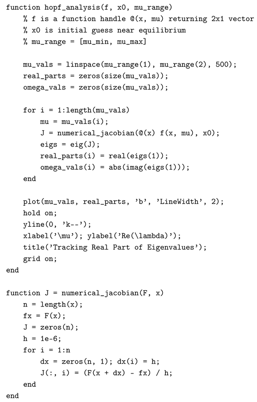
The Hopf bifurcation is a fundamental mechanism for generating periodic orbits. By checking the generic conditions, one can identify and classify such bifurcations analytically and numerically.

We study a linear two-dimensional system depending on a real parameter $\alpha$, showing spiral or rotational motion. This example is particularly insightful as it mimics the behaviour of a Hopf bifurcation in a linear setting.

27. System Description

Consider the system:

$$\begin{array}{cc}\dot{x}=& \alpha x-y\\ \dot{y}=& x+\alpha y\end{array}$$

where $\alpha \in \mathbb{R}$ is a parameter.

28. Matrix Form

This system can be rewritten in matrix form as:

$$\dot{\mathbf{x}}=A\mathbf{x},\mathrm{where}A=\left[\begin{array}{cc}\alpha & -1\\ 1& \alpha \end{array}\right],\mathbf{x}=\left[\begin{array}{c}x\\ y\end{array}\right].$$

29. Eigenvalue Calculation

To analyse the behaviour, compute the eigenvalues $\lambda$ of the matrix A:

$$\begin{array}{cc}\dot{x}=& \alpha x-y\\ \dot{y}=& x+\alpha y\end{array}$$

$$det(A-\lambda I)=\left|\begin{array}{cc}\alpha -\lambda & -1\\ 1& \alpha -\lambda \end{array}\right|={(\alpha -\lambda )}^2+1=0.$$

Solving gives:

$$\lambda =\alpha \pm i.$$

30. Interpretation of Dynamics

The general solution is:

$$x\left(t\right),y\left(t\right)\sim e^{\alpha t}·.$$

Oscillatory terms Therefore:

• $\alpha >0$: Spiral source (unstable).
• $\alpha <0$: Spiral sink (stable).
• $\alpha =0$: Pure centre (closed orbits).

31. MATLAB Visualisation (R2016 Compatible)

Phase Portrait Code:

This linear system exhibits rotational dynamics modulated by exponential growth/decay controlled by $\alpha$. Though linear, it offers a close analogy to Hopf bifurcation at $\alpha =0$.

32. Conclusions

In this study, we have developed a unified analytical framework for understanding bifurcation phenomena in nonlinear and hybrid dynamical systems with biological relevance. By combining local bifurcation theory with explicit constructions of reduced dynamics, we have clarified how qualitative changes in system behaviour arise from variations in key parameters and structural features of the governing equations. In particular, saddle–node, transcritical, and Hopf bifurcations were analysed in a rigorous manner, with precise genericity and non-degeneracy conditions stated explicitly.

A central outcome of this work is the demonstration that complex biological behaviour need not rely on high-dimensional chaos or stochastic forcing. Instead, abrupt transitions, multistability, and oscillatory dynamics can emerge naturally from deterministic mechanisms such as threshold effects, nonlinear feedback, and changes in stability induced by bifurcations. For hybrid and piecewise-defined systems, we have shown that bifurcations are often governed by changes in switching geometry and return-map structure rather than by smooth nonlinear instabilities. This insight provides a mathematically sound explanation for irregular yet bounded dynamics frequently observed in regulatory and physiological systems.

From a biological perspective, the analysis highlights bifurcation theory as a conceptual bridge between molecular-level regulation and system-level behaviour. Fixed-point bifurcations correspond to phenotypic transitions and loss of homeostasis, while Hopf bifurcations offer a principled explanation for the emergence of rhythmic activity in gene expression, population dynamics, and disease transmission. The explicit identification of critical parameter thresholds further suggests how modest biological perturbations may produce disproportionate qualitative effects.

Several limitations should be acknowledged. The models considered here are idealised and deterministic, and do not incorporate stochastic fluctuations, time delays, or spatial heterogeneity that are often present in real biological systems. Consequently, while the bifurcation mechanisms identified provide structural insight, quantitative agreement with experimental data requires further refinement. Future work should focus on extending the analysis to stochastic and delayed systems, validating predicted bifurcation scenarios against experimental observations, and exploring control strategies that exploit bifurcation structure to regulate biological outcomes.

Overall, this work reinforces the central role of bifurcation analysis in mathematical biology, demonstrating its power not only as a diagnostic tool for qualitative change,but also as a framework for interpreting biological complexity through precise mathematical structure.

References

- Shahrear, P.; Glass, L.; Wilds, R.; Edwards, R. Dynamics in piecewise linear and continuous models of complex switching networks . Mathematics and Computers in Simulation 2015, 110, 33–39. [Google Scholar] [CrossRef]
- P Shahrear, L Glass, R Edwards. (2018). Collapsing chaos. Texts in Biomathematics, 35-43.
- Karim, M.D.S.; Shahrear, P.; Rahman, M.D.M.; Ahamad, R. MDS Karim, P Shahrear, MDM Rahman, R Ahamad. Generating formulae for the existing and non-existing numerical integration schemes . Journal of Mathematics and Mathematical Sciences 2005, 21, 91–104. [Google Scholar]
- Shahrear, P.; Faruque, S.B. Shift of the ISCO and gravitomagnetic clock effect due to gravitational spin-orbit coupling . International Journal of Modern Physics D 2007, 16(11), 1863–1869. [Google Scholar] [CrossRef]
- Faruque, S.B.; Shahrear, P. On the gravitomagnetic clock effect . Fizika B: A Journal of Experimental and Theoretical Physics 2008, 17(3), 429–434. [Google Scholar]
- Hussain, F.; Ahamad, R.; Karim, M.S.; Shahrear, P.; Rahman, M.M. Evaluation of Triangular Domain Integrals by use of Gaussian Quadrature for Square Domain Integrals . SUST Studies 2010, 12(1), 15–20. [Google Scholar]
- S H Strogatz. (1994). Nonlinear Dynamics and Chaos: With Applications to Physics, Biology, Chemistry, and Engineering. Boulder, CO: Westview Press.
- L Perko. (2001). Differential Equations and Dynamical Systems (3rd ed.). New York, NY: Springer.
- Shahrear, P.; Rahman, S.M.S.; Nahid, M.M.H. Prediction and mathematical analysis of the outbreak of coronavirus (COVID-19) in Bangladesh . Results in Applied Mathematics 2021, 10, 100145. [Google Scholar] [CrossRef]
- Shahrear, P.; Habiba, U.; Rezwan, S. The Role of the Poincaré Map is Indicating a New Direction in the Analysis of the Genetic Network . International Review on Modelling and Simulations (I.RE.MO.S.) 2022, 15(5), 351–358. [Google Scholar] [CrossRef]
- Faiyaz, C.A.; Shahrear, P.; Shamim, R.A.; Strauss, T.; Khan, T. Comparison of different radial basis function networks for the electrical impedance tomography (EIT) inverse problem . Algorithms 2023, 16(10), 461. [Google Scholar] [CrossRef]
- Das, K.; Srinivas, M.N.; Shahrear, P.; Rahman, S.M.S.; Nahid, M.M.H.; Murthy, B.S.N. Transmission dynamics and control of COVID-19: A mathematical modelling study . Journal of Applied Nonlinear Dynamics 2023, 12(2), 405–425. [Google Scholar] [CrossRef]
- Islam, M.S.; Shahrear, P.; Saha, G.; Ataullah, M.; Shahidur, M.R. Mathematical Analysis and Prediction of Future Outbreak of Dengue on Time-varying Contact Rate using Machine Learning Approach . Computers in Biology and Medicine 2024, 178, 108707. [Google Scholar] [CrossRef]
- Junaid, M.; Saha, G.; Shahrear, P.; Saha, S.C. Phase change material performance in chamfered dual enclosures: Exploring the roles of geometry, inclination angles and heat flux . International Journal of Thermofluids 2024, 24, 100919. [Google Scholar] [CrossRef]
- Shahrear, P.; Islam, M.S.; Bakkar, M.A.; Bushra, A.; Hossain, I. Navigating Epidemic Mathematics: Exploring Tools for Mathematical Modelling in Biology . arXiv 2024, arXiv:2501.00035. [Google Scholar]
- Shahrear, P.; Singha, S.; Tareq, B.; Sharma, Z.; Tanmi, Tasnim. Analysis of the Covid-19 Mathematical Model Based on Vaccine Data: A Descriptive Approach to Eradicate the Outbreak . Preprint 2024. [Google Scholar] [CrossRef]
- AK Saha, G Saha, P Shahrear. (2024). Dynamics of SEPAIVRD model for COVID-19 in Bangladesh. Preprints.
- Junaid, M.; Saha, G.; Shahrear, P.; Saha, S.C. Numerical Evaluation of a Dual Phase Change Material-Integrated Cap for Prolonged Thermal Protection in Extreme Heat . Results in Engineering 2025, 105870. [Google Scholar] [CrossRef]
- Junaid, M.; Shahrear, P.; Habiba, U. Impact of bifurcation angle on hemodynamics and oxygen delivery in stenosed arterial junctions . Physics of Fluids 2025, 37(8). [Google Scholar] [CrossRef]
- G Saha, P Shahrear, A Faiyaz, AK Saha. (2025). Mathematical Modeling of Lumpy Skin Disease: New Perspectives and Insights. Partial Differential Equations in Applied Mathematics, 101218.
- Saha, G.; Shahrear, P.; Rahman, S.; Nazi, R.; Srinivas, M.N.; Das, K. Climate change potential impacts on mosquito-borne diseases: a mathematical modelling analysis . Tamkang Journal of Mathematics 2025, 56(3), 335–354. [Google Scholar] [CrossRef]
- Rahman, S. M. S..; Samanta, F..; Shahrear, P.. Analysis of COVID-19 Disease Transmission: A Blended Appraisal of Quarantine and Vaccination Effects in Bangladesh . GORTERIA 2025, 65(7), 32–24. [Google Scholar] [CrossRef]
- Mohammad, J..; Shahrear, P..; Chowdhury Ruhel, F.. Analysis of COVID-19 Disease Transmission: A Blended Appraisal of Quarantine and Vaccination Effects in Bangladesh . Journal of Advanced Research in Numerical Heat Transfer 2025, 31(1), 126–150. [Google Scholar]
- Shahrear, P. and Habiba, U. and Islam, M. D. S. and Hussain, F. and Saha, G. (2025). Tracking the Rhythm of Heat: Seasonal SEIR Modelling and Machine Learning for Heat Wave Forecastingh. Preprint.
- Shahrear, P. and Saiki, M. F. H. and Nabi Tareq, M. T. (2024). Analysis of COVID-19 Data Based on Modelling and Descriptive Statistical Approach. Preprint Manuscript.
- H Kielhöfer. (2012). Bifurcation Theory: An Introduction with Applications to Partial Differential Equations. New York, NY: Springer. :contentReference[oaicite:0]index=0.
- S-N Chow, J K Hale. (1982). Methods of Bifurcation Theory. New York, NY: Springer. :contentReference[oaicite:1]index=1.
- Y A Kuznetsov. (2023). Elements of Applied Bifurcation Theory. Cham, Switzerland: Springer. :contentReference[oaicite:2]index=2.
- I G Vardoulakis, J Sulem. (1995). Bifurcation Analysis in Geomechanics. Boca Raton, FL: CRC Press. :contentReference[oaicite:3]index=3.
- H A Dijkstra, F W Wubs. (2023). Bifurcation Analysis of Fluid Flows. Cambridge: Cambridge University Press. :contentReference[oaicite:4]index=4.
- J-Q Sun, A C J Luo (Eds.). (2006). Bifurcation and Chaos in Complex Systems, Volume 1. Amsterdam: Elsevier. :contentReference[oaicite:5]index=5.
- F Seydel, F W Schneider, T Küpper, H Troger (Eds.). (1991). Bifurcation and Chaos: Analysis, Algorithms, Applications. Basel: Birkhäuser. :contentReference[oaicite:6]index=6.
- A G Wilson. (1981). Catastrophe Theory and Bifurcation: Applications to Urban and Regional Systems. London: Routledge. :contentReference[oaicite:7]index=7.
- A C J Luo. (2019). Bifurcation and Stability in Nonlinear Dynamical Systems. Cham, Switzerland: Springer. :contentReference[oaicite:8]index=8.
- J C Alexander, J A Yorke. (1978). Global bifurcations of periodic orbits. American Journal of Mathematics, 100(2), 263–292. Providence, RI: American Mathematical Society. :contentReference[oaicite:0]index=0.
- M J Feigenbaum. (1978). Quantitative universality for a class of nonlinear transformations. Journal of Statistical Physics, 19(1), 25–52. Dordrecht: Springer Netherlands. :contentReference[oaicite:1]index=1.
- M J Feigenbaum. (1979). The onset spectrum of turbulence. Physics Letters A, 74(6), 375–378. Amsterdam: Elsevier. :contentReference[oaicite:2]index=2.
- M J Feigenbaum. (1980). The transition to aperiodic behavior in turbulent systems. Communications in Mathematical Physics, 77(1), 65–86. Berlin: Springer. :contentReference[oaicite:3]index=3. Berlin.
- S N Chow, J Mallet-Paret. (1977). Integral averaging and Hopf’s bifurcation. Journal of Differential Equations, 26(1), 112–159. New York, NY: Academic Press. :contentReference[oaicite:4]index=4.
- S N Chow, J Mallet-Paret. (1978). The Fuller index and global Hopf bifurcations. Journal of Differential Equations, 29(1), 66–85. New York, NY: Academic Press. :contentReference[oaicite:5]index=5.
- J Mallet-Paret, J A Yorke. (1982). Snakes: oriented families of periodic orbits, their sources, sinks and continuation. Journal of Differential Equations, 43(3), 419–450. New York, NY: Academic Press. :contentReference[oaicite:6]index=6.
- Shahrear, P.; Glass, L.; Edwards, R. Chaotic dynamics and diffusion in a piecewise linear equation . Chaos: An Interdisciplinary Journal of Nonlinear Science 2015, 25(3). [Google Scholar] [CrossRef]
- P Shahrear, L Glass, N Del Buono. (2015). Analysis of Piecewise Linear Equations with Bizarre Dynamics. Ph.D. Thesis, Department of Mathematics, 135.
- Chakraborty, A.K.; Shahrear, P.; Islam, M.A. Analysis of epidemic model by differential transform method . J. Multidiscip. Eng. Sci. Technol 2017, 4(2), 6574–6581. [Google Scholar]
- MA Islam, MA Sakib, P Shahrear, SMS Rahman. (2017). The Dynamics of Poverty, Drug Addiction and Snatching In Sylhet, Bangladesh.
- Sakib, M.; Islam, M.; Shahrear, P.; Habiba, U. Dynamics of poverty and drug addiction in Sylhet, Bangladesh . Dynamics 2017, 4(2). [Google Scholar]
- Rahman, S.M.S.; Islam, M.A.; Shahrear, P.; Islam, M.S. Mathematical Model on Branch Canker Disease in Sylhet, Bangladesh . Journal of Mathematics 2017, 13(1 Ver. IV), 80–87. [Google Scholar]
- Shahrear, P.; Chakraborty, A.K.; Islam, M.A.; Habiba, U. Analysis of computer virus propagation based on compartmental model . Applied and Computational Mathematics 2018, 7(1-2), 12–21. [Google Scholar]
- Ahamad, R.; Karim, M.S.; Rahman, M.M.; Shahrear, P. Finite element formulation employing higher order elements and software for one dimensional engineering problems . SUST Journal of Science and Technology 2019, 29(1), 1–16. [Google Scholar]
Disclaimer/Publisher’s Note: The statements, opinions and data contained in all publications are solely those of the individual author(s) and contributor(s) and not of MDPI and/or the editor(s). MDPI and/or the editor(s) disclaim responsibility for any injury to people or property resulting from any ideas, methods, instructions or products referred to in the content. |
© 2025 by the authors. Licensee MDPI, Basel, Switzerland. This article is an open access article distributed under the terms and conditions of the Creative Commons Attribution (CC BY) license (http://creativecommons.org/licenses/by/4.0/).
Copyright: This open access article is published under a Creative Commons CC BY 4.0 license, which permit the free download, distribution, and reuse, provided that the author and preprint are cited in any reuse.