Detecting all Homoclinic Points in Nonlinear Discrete Dynamical Systems Via Resurgent Analysis

1. Introduction

In 1890, Poincaré proved that the three-body problem in celestial mechanics is non-integrable and the solution cannot be described by any existent function [1]. He introduced a geometrical concept called homoclinic points for the proof and showed that, if a dynamical system has one (transverse) homoclinic point, then an infinite number of homoclinic points exist in the system. Mathematically, homoclinic points are represented as intersections of the stable and unstable manifolds emerging from fixed or periodic points in a given dynamics [2]. The set of homoclinic points is a geometrical representation of chaos that yields a corresponding configuration in the phase space, which possesses a fractal structure [3,4]. If one can detect the set of homoclinic points, all the quantities of a given dynamical system such as the entropy, Hausdorff (fractal) dimension, Lyapunov exponent, etc. can be obtained whenever the dimension of the phase space is less than three.

Following the discovery of homoclinic points by Poincaré, the ergodic theory was developed by Birkhoff, von Neumann, and Sinai et al. [5,6,7], which is also a geometrical construct. Smale, Ruelle, and Bowen formulated a stochastic analysis technique for chaos, which is based on a geometrical representation [8,9,10]. Barreira and Pesin proved that an abstract concept known as Kolmogorov-Sinai entropy is equivalent to the Lyapunov exponent in chaotic regions, and connected this purely mathematical concept to the corresponding physical quantity [11]. Recently, Koda, Hanada, and Shudo provided the relationship between Kolmogorov-Sinai entropy on Julia sets of polynomial maps and quantum tunneling [12]. These studies are all essentially stochastic and were constructed under the assumption that the integral manifold does not exist, as this characteristic indicates the appearance of chaos. To date, the deterministic approach to chaos has involved the time-series analysis technique only [13,14]; however, this approach is suitable for short-term analysis only, and the accuracy of the time-series analysis deteriorates significantly for long-term calculations.

On the contrary to the time-series analysis, the set of homoclinic points involves every event extending from the past into future in a dynamical system, and therefore, one can calculate chaotic trajectories deterministically provided that all homoclinic points are found. The sea of chaos following the collapse of the KAM torus is a well-known and typical example of the set of homoclinic points [15,16]. Usually, homoclinic points are obtained by perturbing the integrable Hamiltonian systems such that the stable manifold coincides with the unstable one. Detection of homoclinic points has been performed only by qualitative methods as Melnikov integral [15,16]. This method is effective to show the existence of homoclinic points mathematically; however, it is unsuitable for numerical computations and inapplicable to physics.

Tovbis was the first to estimate quantitatively a homoclinic point [17]. He succeeded to calculate the splitting angle between the stable and unstable manifolds in the Hénon map for the case in which the system becomes the Hamiltonian system and showed the transversality at a homoclinic point numerically by using the Borel-Laplace transform. In the same dynamical system, Gelfreich and Sauzin have found a homoclinic point with higher accuracy than that given by Tovbis [18] using the resurgent analysis [19,20,21]. Anastassiou, Bountis, and Bäcker [22] calculated a few homoclinic points using the classical linearized function presented by Poincaré [23]. This linearized function is given by the Taylor expansion around a fixed point, and the accuracy rapidly deteriorates when we consider points far from the fixed point. Therefore, it is not suitable for quantitative calculations. As the set of homoclinic points is a purely mathematical concept, concrete calculation of this set is extremely difficult.

In this article, we present a method for calculating the full set of homoclinic points in a dynamical system, using an analytic function that represents the stable and unstable manifolds of the system and taking a quadratic map as an example. The method adopted here, which is an extension of the resurgent analysis described above, is mathematically rigorous, and no approximation is required. We also provide a numerical scheme that permits visualization of the set of homoclinic points, so that it can be treated as an ordinary function. The set of obtained points represents the solution to a non-integrable system and corresponds to an integral manifold in integrable systems. Identification of the set of homoclinic points indicates that every event extending from the past into future can be determined. If one can calculate all homoclinic points concretely, it becomes possible to model chaos and to make long-term predictions. In one-dimensional dynamical systems, the closure of the set of homoclinic points coincides with the Julia set [24] where the trajectories of dynamical systems are chaotic [25,26,27,28]. We verify this fact by an experimental mathematical approach (multiple-precision calculation) and discuss the extensibility to higher-dimensional dynamical systems where the configuration of homoclinic points is unknown.

This paper is organized as follows. In Section 2, we introduce the difference equation that derived from the quadratic map and present the solution to the difference equation in an asymptotic expansion form. This solution can describe the unstable manifold of the quadratic map. In Section 3, we estimate the number of zeros of the function adopted to capture the homoclinic points. In Section 4, we present an algorithm for the detection of zeros of the function describing the unstable manifold. Numerical results for the distribution of the zeros and the configuration of the set of homoclinic points are provided in Section 5. Section 6 is devoted to concluding remarks.

2. Basic Concepts of Homoclinic Points and Governing Equations

We consider a state $x=x\left(t\right)$ that is parameterized by time t ($t\in \mathbb{C}$) and denote the stable and unstable manifolds as $x=x_s$ and $x=x_u$, respectively [29,30,31]. Then, the set of homoclinic points, which is the intersection of $x=x_s$ and $x=x_u$, is generally represented by the equation

$$x_s\left(t_s\right)-x_u\left(t_u\right)=0,$$

where $t=t_s$ and $t=t_u$ are the times parameterizing $x=x_s$ and $x=x_u$, respectively. When the system is one-dimensional, $x_s\left(t_s\right)=0$ and, therefore, the above equation is reduced to

$$x_u\left(t_u\right)=0.$$

This indicates that, in order to obtain the set of homoclinic points, the zeros of $x_u$ must be calculated. From now on, we drop the subscript u in $x_u\left(t_u\right)$.

We now introduce a nonlinear map f that describes a physical phenomenon, and consider a transform such that the n-th iteration ($n\ge 0$, $n\in \mathbb{Z}$) of f is given by a shift in the t plane: [32]

$$\begin{array}{c}\hfill f^n\circ x\left(t\right)=x(t+n),\end{array}$$

(1)

where $f\left(x\right)$ is assumed to be a polynomial for x. As a prototype of chaotic dynamical systems, we adopt the quadratic map

$$\begin{array}{c}\hfill f\circ x\left(t\right)=1-ax{\left(t\right)}^2,\end{array}$$

(2)

where a is a dynamical parameter. One of the (hyperbolic) fixed points

$$x_f={\displaystyle \frac{-1+\sqrt{1+4a}}{2a}}$$

is shifted to the origin according to $x\to x+x_f$, and the quadratic map is then given by

$$\begin{array}{c}\hfill f\circ x\left(t\right)=-2a{x}_{f}x\left(t\right)-ax{\left(t\right)}^2.\end{array}$$

(3)

From (1) and (3), we obtain the difference equation

$$\begin{array}{c}\hfill x(t+1)=-2a{x}_{f}x\left(t\right)-a{\left[x\left(t\right)\right]}^2.\end{array}$$

(4)

By performing the Laplace transform of $x\left(t\right)$, which is based on the resurgent analysis [18,19,20,21], we obtain the following asymptotic expansion representation as a global solution to the equation (4) [32,33]:

$$\begin{array}{c}\hfill x\left(t\right)=\sum _{N=1}^{\infty }{\displaystyle \frac{b_N(N-1)!,e^{N{\zeta }_{1}t}}{{(t+n_0)}^N}}\left[1+O\left(\right|t+n_0{|}^{-1})\right],\end{array}$$

(5)

where $n_0$, a large positive integer, is an artificial parameter used to increase the accuracy of the asymptotic expansion, ${\zeta }_1=ln\left|\alpha \right|-\pi i$, $\alpha$ ($\alpha \ne 0$) is the eigenvalue of the map that satisfies $\left|\alpha \right|>1$ (hyperbolic, $\alpha <0$ here), i is the imaginary unit, and the coefficient $b_N$ satisfies the recurrence formula

$$\begin{array}{c}\hfill b_N=-{\displaystyle \frac{2a}{D_N}}\sum _{k=1}^{N-1}\sum _{r=0}^{N-k-1}{b}_k{b}_{N-k}{\displaystyle \frac{(N-k-1)!{(-1)}^r{\left(k/N\right)}^{k+r}}{(N-k-1-r)!r!(k+r)}},\end{array}$$

(6)

in which $D_N={\alpha }^N+2a{x}_f$ and the initial value $b_1$ is selected as $b_1=x_f/2$. Here, the coefficient $b_N$ is estimated as [33]

$$|b_N|\le {\displaystyle \frac{K^N{\left|\alpha \right|}^{-NlogN}}{N!}}$$

for $\left|\alpha \right|>1$, where $K>1$ is a constant. This estimate guarantees the suppression of divergence of the factor $e^{N{\zeta }_{1}t}(N-1)!$ for $\Re \left({\zeta }_{1}t\right)>0$ in (5).

Since the function $x\left(t\right)$ in (5) is represented by an asymptotic expansion, it describes the stable and unstable manifolds realized at $t=\pm \infty$ very accurately [33]. The value $t=-n_0$ in (5) is merely a cosmetic singularity, and it is possible to expand $x\left(t\right)$ for any value of t ($t\in \mathbb{C}$). The asymptotic expansion (5) can describe various dynamical quantities in nonlinear systems very precisely [32,34]. Further, the expansion (5) is a mathematically rigorous solution to the difference equation (4), and no approximation is applied to derive the former expression [33]. The only equation used to calculate the set of homoclinic points is (5), which incorporates the deterministic coefficient given in (6). We calculate the set of homoclinic points as zeros of the function $x\left(t\right)$ as accurately as possible and visualize the results via a computational representation. In the following, we set the positive integer $n_0={10}^5$ and drop the higher order term of $O\left(|t+n_0{|}^{-(N+1)}\right)$ from (5).

3. Distribution of Zeros in the Complex Plane

The equation $f\circ x\left(t\right)=0$ in (3) [or (2)] has two roots corresponding to simple zeros, from which, we see that the zeros of $f^n\circ x\left(t\right)=x(t+n)=0$ are given by $2^n$ points

$$\begin{array}{c}\hfill x=x_1,x_2,\dots ,x_{2^n}.\end{array}$$

(7)

When $\left|t\right|$ is large, the function $x\left(t\right)$ oscillates very rapidly [32], which provides the zeros as much as the number of times of oscillations. We estimate the values of t that provide these zeros.

Theorem 1. 

Let $J\left(f\right)$ be the Julia set of the nonlinear map f. Then there exists some constant $M>0$ ($M\in \mathbb{R}$) such that

$$\begin{array}{c}\hfill \left\{x\right(t)\mid |\Re \left(t\right)|,|\Im \left(t\right)|\le M\}\supset J\left(f\right).\end{array}$$

(8)

holds.

Proof. 

The Julia set $J\left(f\right)$ is an infinite set and therefore, there exists some constant $t_0\in \mathbb{C}$ such that $x\left(t_0\right)\in J\left(f\right)$ holds. Let U be an open neighborhood of $t_0$. Then $x\left(U\right)$ is an open set intersecting $J\left(f\right)$ and there exists $n\in \mathbb{N}$ such that $f^n\left(x\left(U\right)\right)\supset J\left(f\right)$ holds [24,27]. Since $f^n\circ x\left(t\right)=x(t+n)$, we have

$$\begin{array}{c}\hfill x(U+n)\supset J\left(f\right).\end{array}$$

(9)

Choose $M>0$ such that

$$U+n\subset \{t\in \mathbb{C}\mid |\Re \left(t\right)|,|\Im \left(t\right)|\le M\}.$$

Then the theorem is obtained.

□

For $M>0$ and $n\ge 0$ ($n\in \mathbb{Z}$), we define

$$\begin{array}{ccc}\hfill B(n,M)& =& \{t\in \mathbb{C}\mid |\Re (t-n)|,|\Im (t-n)|\le M\},\hfill \\ \hfill z(n,M)& =& \{t\in B(n,M)\mid x(t)=0\}.\hfill \end{array}$$

Let ♯ denote the cardinality. For the number of zeros of $x\left(t\right)$, the following theorem holds.

Theorem 2. 

There exists a constant $M>0$ such that

$$\begin{array}{c}\hfill \underset{n\to \infty }{lim}{\displaystyle \frac{1}{n}}log♯z(n,M)=log2\end{array}$$

(10)

holds.

Proof. 

Let M be as in Theorem 1. Since 0 is an expanding fixed point of f, we have $0\in J\left(f\right)$. Note that the Julia set $J\left(f\right)$ is completely invariant under f; i.e.,

$$f\left(J\left(f\right)\right)=f^{-1}\left(J\left(f\right)\right)=J\left(f\right).$$

As $f^{-n}\left(J\left(f\right)\right)=J\left(f\right)$, we have $x_1^n,x_2^n,\dots x_{2^n}^n$ such that

$$f^{-n}\left(0\right)=\{x_1^n,x_2^n,\dots x_{2^n}^n\}\subset J\left(f\right).$$

From Theorem 1, there exist $t_1^n,t_2^n,\dots t_{2^n}^n$$\in B(0,M)$ such that

$$x\left(t_i^n\right)=x_i^n(i=1,2,\dots 2^n),$$

which satisfy

$$\begin{array}{c}\hfill f^n\circ x\left(t_i^n\right)=x(t_i^n+n)=0.\end{array}$$

Therefore,

$$t_i^n+n\in z(n,M).$$

The multiple root; $x_i^n=a{x}_f^2$ [refer to (17)] occurs at most once in $i=1,2,\dots 2^n$ and all n. Then the number of roots $2^n$ reduces to at most $2^{n-1}$. Therefore,

$$\begin{array}{c}\hfill ♯z(n,M)\ge 2^n-2^{n-1}.\end{array}$$

(11)

The number of $t_i^n$ that satisfies $x\left(t_i^n\right)=x_i^n$ is at most $p\in \mathbb{N}$ for a fixed M when t is restricted on $B(0,M)$. Thus, we obtain

$$\begin{array}{c}\hfill ♯z(n,M)\le p{2}^n.\end{array}$$

(12)

From (11) and (12), the theorem is obtained.

□

In the current study, we detect these zeros with the assistance of a computer.

Remark 1. 

The number of zeros in well-known classical entire functions that appear as solutions to the linearization of nonlinear maps [22,23,29,30,31] is usually polynomial order. The fact that the number of zeros is exponential order enables us the computation of the set of homoclinic points.

4. Properties of Adopted Function and Algorithm for Computations

As stated in Theorem 2 of the previous section, the number of zeros increases as $\Re \left(t\right)$ becomes large. Therefore, it is desirable to select the value of $\Re \left(t\right)$ as large as possible to capture more homoclinic points. To detect the zeros of $x\left(t\right)$, we use the Newton’s method. In the function adopted here, $\left|x\right(t\left)\right|$ for $\Re \left(t\right)\gg 1$ is very large [$\sim O\left({10}^{1000}\right)$ for selected t], while the ratio between $\left|x\right(t\left)\right|$ and its derivative $d\left|x\right(t\left)\right|/dt$ is exponentially small. This indicates that the value of t hardly moves and the convergence of the Newton’s method is extremely slow. Therefore, it is difficult to capture the homoclinic points (zeros of the function) only by the conventional Newton’s method. We show this in subSection 4.1. In subSection 4.2, we present an acceleration scheme to converge the Newton’s method in the fewest times as possible.

4.1. Estimation of Initial Values

In this subsection, we estimate the initial magnitude of the function $x\left(t\right)$ and the number of initial zeros prior to implementing the Newton’s method. The zeros of $x\left(t\right)\in \mathbb{C}$ is calculated by using the Newton’s method as

$$\begin{array}{c}\hfill t_{k+1}=t_k-{\displaystyle \frac{x\left(t_k\right)}{x^{\prime }\left(t_k\right)}},\end{array}$$

(13)

where $t_k\in \mathbb{C}$ ($k=1,2,\dots$) is the discretized variable of t and the prime denotes the differentiation with respect to t. Since $x\left(t\right)$ is Laplace transformable (and hence $x^{\prime }\left(t\right)$ is also Laplace transformable), it is guaranteed that the growth at $t=\infty$ is at most exponential order [35]. In Figure 1 (a), we numerically show an example of the initial amplitude of $x\left(t\right)$ before implementing the Newton’s method, where the dynamical parametr $a=1.9408$. We see that the difference between $\left|x\right(t_{k+1}\left)\right|$ and $\left|x\right(t_k\left)\right|$ is extremely large (e.g. more than ${10}^{10}$) when $\Re \left(t_k\right)$ is large. From this figure, we can expect that the growth of $x\left(t\right)$ is

$$\begin{array}{c}\hfill \left|x\left(t\right)\right|\sim e^{c_0\left|t\right|}(c_0>0,c_0\in \mathbb{R}).\end{array}$$

(14)

The derivative $x^{\prime }\left(t\right)$ also has the same growth as (14).

Figure 1. (a) Initial amplitude of $x\left(t\right)$ and (b) the ratio $\left|x\left(t\right)\right|/|x^{\prime }\left(t\right)|$ plotted by log scale, where the holizontal axis denotes the real part of t and we select a as $a=1.9408$.

Figure 1. (a) Initial amplitude of $x\left(t\right)$ and (b) the ratio $\left|x\left(t\right)\right|/|x^{\prime }\left(t\right)|$ plotted by log scale, where the holizontal axis denotes the real part of t and we select a as $a=1.9408$.

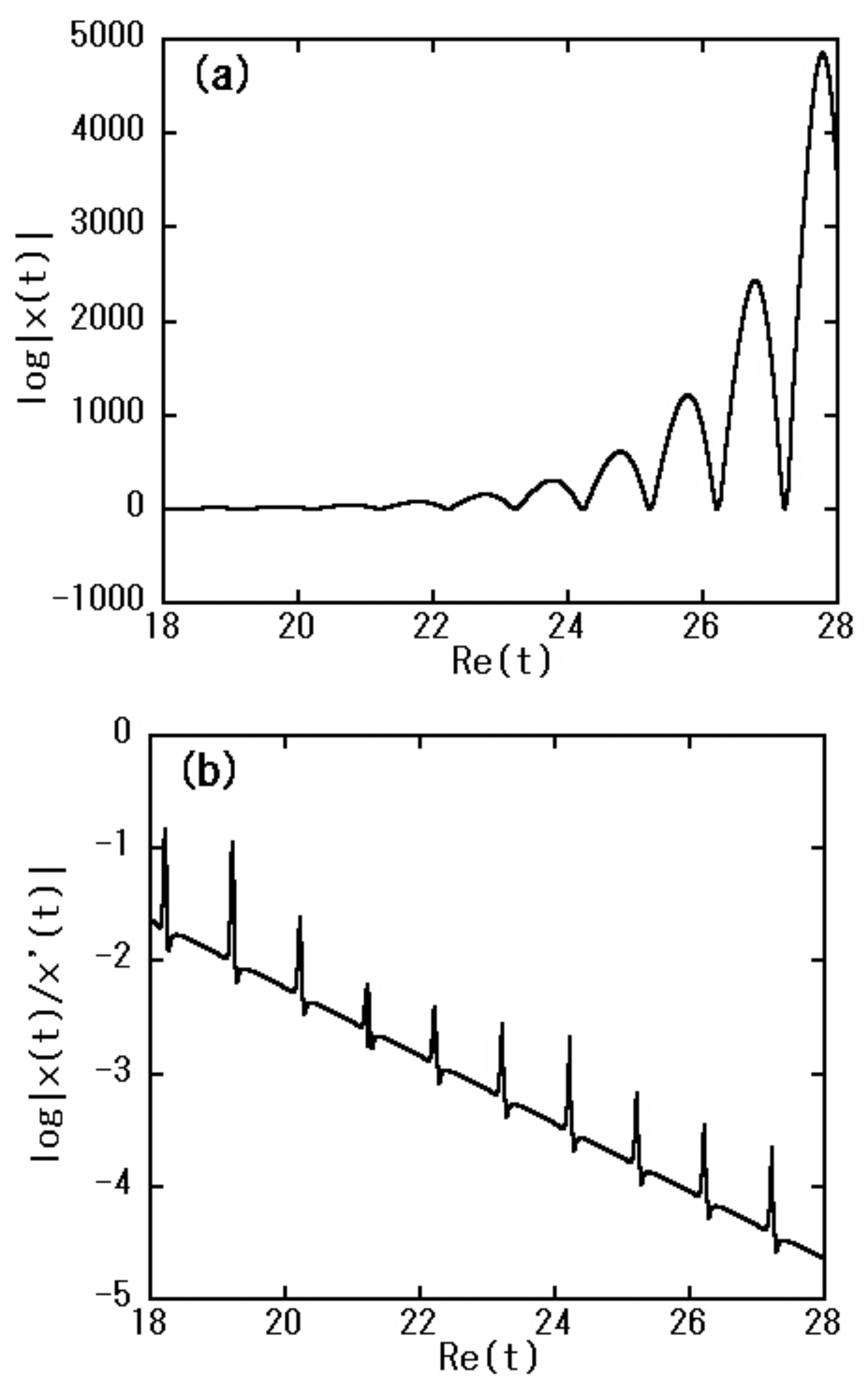
The magnitude of the ratio $|x\left(t\right)/x^{\prime }\left(t\right)|$ on the right hand side of (13) is shown in Figure 1 (b). Using (1), we have

$$\begin{array}{c}\hfill [f^{\prime }\circ x\left(t\right)]x^{\prime }\left(t\right)=x^{\prime }(t+1).\end{array}$$

(15)

From (3), (14), and (15), we can estimate the ratio $|x\left(t\right)/x^{\prime }\left(t\right)|$ as

$$\begin{array}{c}\hfill \left|{\displaystyle \frac{x\left(t\right)}{x^{\prime }\left(t\right)}}\right|\sim \left|{\displaystyle \frac{x^{\prime }(t+1)}{{\left[x^{\prime }\left(t\right)\right]}^2}}\right|\sim c_1{e}^{-c_2\left|t\right|},\end{array}$$

(16)

for some constants $c_1$ and $c_2$ ($>0$, $c_1,c_2\in \mathbb{R}$). Figure 1 (b) supports this estimate. Estimation (16) shows that the difference $|t_{k+1}-t_k|$ in (13) is exponentially small despite the magnitude of $x\left(t\right)$. This fact makes it difficult to converge the Newton’s method. In the neighborhood of cusps in Figure 1 (b) where the derivative $|x^{\prime }\left(t\right)|$ is very small compare to $\left|x\right(t\left)\right|$, the difference $|t_{k+1}-t_k|$ in (13) is relatively large and the candidates of first zeros (“seeds", refer to subSection 4.2) appear after a few implementations of the Newton’s method.

From the fact that the value of $log\left|x\right(t\left)\right|$ in Figure 1 (a) and $log|x\left(t\right)/x^{\prime }\left(t\right)|$ in Figure 1 (b) are finite, we find that there is no zero in $x\left(t\right)$ before the implementations of the Newton’s method. There exist various acceleration methods in the conventional Newton’s method to speed up the convergence [36]; however, these methods can only apply to the case that $|x\left(t_k\right)/x^{\prime }\left(t_k\right)|$ in (13) is polynomial order with respect to t [37]. Therefore, another way is required to accelerate the convergence of the Newton’s method in the current study. We present the method in the next subsection.

4.2. Algorithm for Detecting Zeros

The set of homoclinic points is the set of points that are at the fixed point at $t=-\infty$ (distant past) and that return to the fixed point at $t=\infty$ (distant future). The behavior of $x\left(t\right)$ given by (5) is violent for $\left|t\right|\gg 1$ (distant future), where a large number of zeros exist [32]. We define the time corresponding to the distant future as $t=t_r+i{t}_i$ ($27\le t_r\le 28$), where the imaginary part $t_i$ is selected appropriately depending on the value of a. As regards the value of $t_r$, the larger the better. The range $27\le t_r\le 28$, where we detect the zeros of $x\left(t\right)$, is the only limit of our computation, and the actual value itself is non-critical. In order to find the zeros of $x\left(t\right)$, we adopt the Newton’s method with a certain acceleration. Generally, the values of $\left|x\right(t\left)\right|$ are very large when $t_i>0$, and the typical values of $\left|x\right(t\left)\right|$ calculated here are within $\left|x\left(t\right)\right|>O\left({10}^{100}\right)\sim O\left({10}^{5000}\right)$ for almost all a$(\ge 1.0)$. The conventional Newton’s method and the typically applied double-precision calculation are not useful as regards determine the zeros for such large values of $x\left(t\right)$. In this subsection, we present an acceleration scheme to converge the Newton’s method for a function such that its absolute value is very large and the difference $|t_{k+1}-t_k|$ in (13) is exponentially small. The algorithm to find the zeros of $x\left(t\right)$ is as follows.

1.

Calculate the coefficient $b_N$ given by (6) in advance. Here, we truncate the upper limit N in (6) by setting $N=1000$.

2.

Divide the region $t=t_r+i{t}_i$ ($27\le t_r\le 28$, $t_i$, fixed) into $1/K_0$ parts and calculate the value of $x\left(t\right)$ for each t. The initial number of partitions $K_0$ is selected so that it almost coincides with the number of oscillations of $x\left(t\right)$ in the $27\le t_r\le 28$ region. This number of oscillation corresponds to zeros of $x\left(t\right)$. Here, we set $K_0$ to 2000. For $x\left(t\right)$, we implement Newton’s method once only for each t.

3.

Set the initial values before and after Newton’s method is implemented once as $t=t_0\left(k\right)$ and $t=t_1\left(k\right)$ ($k=1,2,\dots K$), respectively. During the Newton’s method calculation, we remove the values of t such that they satisfy $|x\left(t_1\right)|>|x\left(t_0\right)|$. Therefore, the value of K (the number of partitions after the implementation of the Newton’s method) is always smaller than $K_0$.

4.

Detect the values of $t_1={\tilde{t}}_1\left(m\right)$ ($m=1,2,\dots M_s$) in $t_1\left(k\right)$ ($k=1,2,\dots K$) such that $\left|x\right({\tilde{t}}_1\left(m\right)\left)\right|<L$ is satisfied, where L is a relatively small integer ($L=100$ in this study). The value of $M_s$ is generally small ($M_s\ll K$) after Newton’s method is implemented for the first time. We refer to the ${\tilde{t}}_1\left(m\right)$ ($m=1,2,\dots M_s$) as “seeds".

5.

Calculate the distance between the seeds as $d(k,m)\equiv |t_1\left(k\right)-{\tilde{t}}_1\left(m\right)|$ for all k ($k=1,2,\dots K$) and m ($m=1,2,\dots M_s$) and detect the minimum value with respect to each k, $d_{min}\left(k\right)$, for all m.

6.

Calculate the acceleration coefficient $\beta \left(k\right)\equiv d_{min}\left(k\right)/|t_1\left(k\right)-t_0\left(k\right)|$ ($k=1,2,\dots K$), where we set $\beta \left(k\right)=1$ when $d_{min}\left(k\right)=0$.

7.

Calculate the next initial values $t=t_2$ as $t_2\left(k\right)=\beta \left(k\right)[t_1\left(k\right)-t_0\left(k\right)]+t_0\left(k\right)$, reset to $t_0\left(k\right)=t_2\left(k\right)$, and perform the next Newton’s method calculation.

The processes $1-2$ are initial settings. We repeat the above processes $3-7$ until each value of $x\left(t\right)$ tends to zero [less than $O\left({10}^{-30}\right)$; the tolerance level adopted here]. We refer to processes $4-6$ as the “acceleration." The seeds are the points that are located in the neighborhood of zeros of $x\left(t\right)$ and the acceleration coefficient $\beta$ is greater than one when the points are far from the seeds. The number of seeds $M_s$ increases as repeatedly implement both Newton’s method and the acceleration, and finally, $M_s=K$ holds as a result of the acceleration after the final implementation of Newton’s method. This final $M_s$ provides the number of zeros.

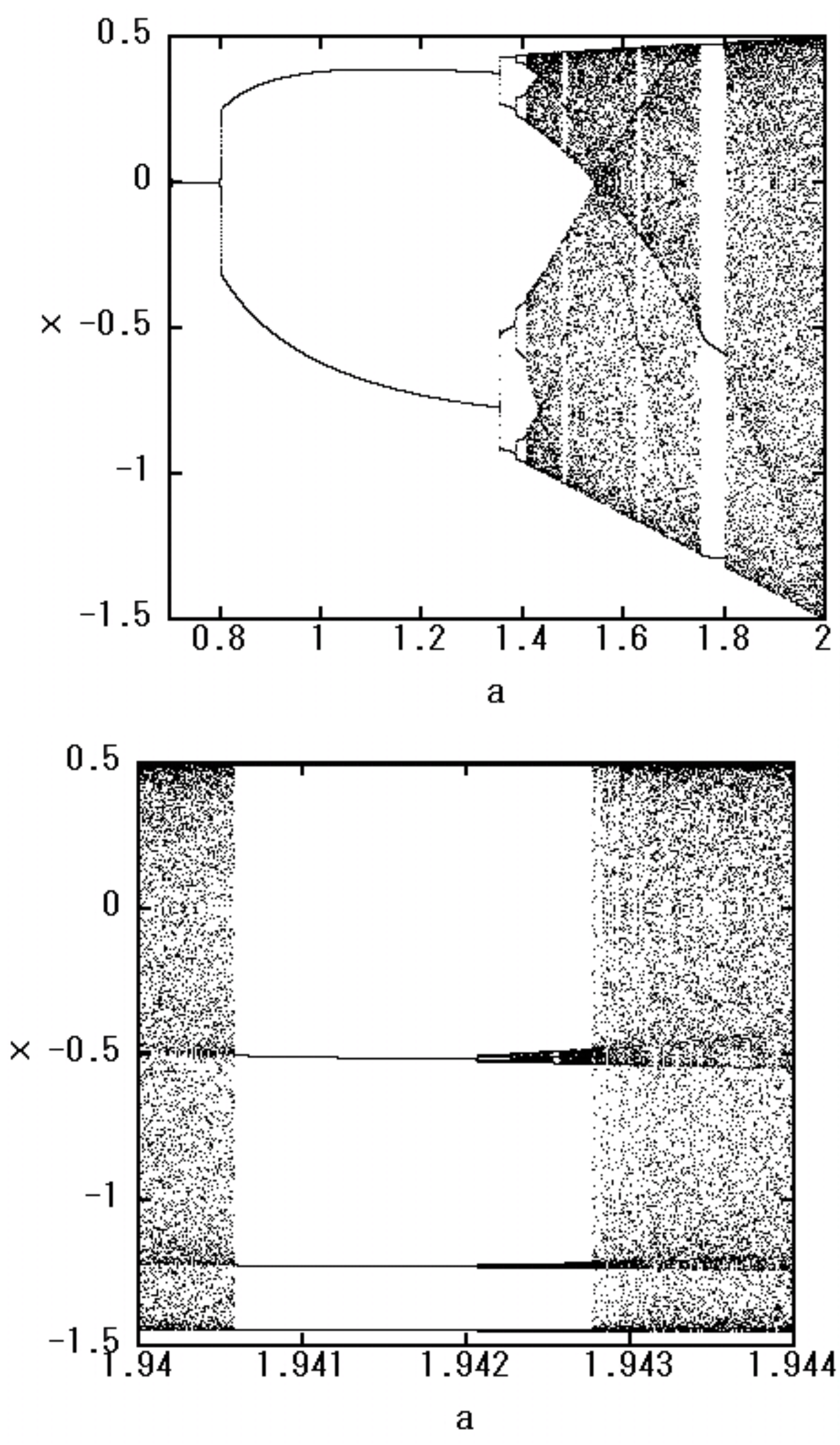
Figure 2. Bifurcation diagram of the quadratic map (3), where the lower figure enlarges the parameter region $1.940\le a\le 1.944$ in the upper figure. The value of x moves in the range $-1.5\le x\le 0.5$ in our normalization.

Figure 2. Bifurcation diagram of the quadratic map (3), where the lower figure enlarges the parameter region $1.940\le a\le 1.944$ in the upper figure. The value of x moves in the range $-1.5\le x\le 0.5$ in our normalization.

The number of implementations of Newton’s method required to reach $\left|x\left(t\right)\right|<O\left({10}^{-30}\right)$ depends on the value of the dynamical parameter a in (2) and the value of t, and becomes larger as a increases. By adopting the acceleration, almost all values of $\left|x\right(t\left)\right|$ with $O\left({10}^{1000}\right)$ decrease up to the level of $O\left(1\right)$ after $10-15$ implementations of Newton’s method. If the acceleration process is not employed, the value of $\left|x\right(t\left)\right|$ with $O\left({10}^{1000}\right)$ remains at the level of $O\left({10}^{400}\right)\sim O\left({10}^{500}\right)$, even after 20 implementations of Newton’s method, and this value decreases only minimally, despite the fact that we continue to implement Newton’s method.

All calculations in processes $2-7$ are performed with multiple precision (150 digits here) to avoid the round-off error. The process 1 only is performed with 500 digits in order to take the coefficients of the asymptotic expansion (6) accurately as many as possible.

5. Numerical Results

As stated in the introduction, it is mathematically known that the set of homoclinic points coincides with the Julia set in one-dimensional dynamical systems. In this section, we show this fact numerically by calculating the homoclinic points of the function $x\left(t\right)$.

The chaotic region is specified by the bifurcation diagram of the nonlinear map f. Iterative calculation of the quadratic map (3) provides Figure 2, where $a\ge 1.4$ is fully chaotic region, at least, as long as we consider the real x. There exist non-chaotic regions called “windows" in this fully chaotic region. These window regions exhibit events that rarely occur but are physically important and it is known to be difficult to calculate dynamical quantities such as the entropy or Lyapunov exponent in those regions because there exists no physically observable measure in the window regions. We show one of the window regions in the lower figure of Figure 2. The orbit realized in the real space is not chaotic in this region; however, the same complexity as the chaotic region ought to exist there. The set of homoclinic points can capture the complexity precisely. We show that in the subsequent subsections, taking $a=1.9408$ (a point in the window of fully chaotic region) as an example. When $a<1.4$, the orbit is non-chaotic in the real space. However, the behavior in the complex plane is completely different. We also present the complexity in the complex plane of the dynamical system such that it is periodic in the real space, taking $a=1.0$ (a point in the periodic region) as an example.

5.1. Effects of acceleration

In this subsection, we estimate the acceleration method stated in Section 4.2. Figure 3 shows the distribution of t such that the value of $x\left(t\right)$ tends to $x\left(t\right)=0$ for the Newton’s method with acceleration stated in Section 4.2, where we select $a=1.9408$. This value of a belongs to a window in the fully chaotic region (refer to Figure 2). The initial time (distant future) $t=t_r+i{t}_i$ is selected as $27\le t_r\le 28$ and $t_i=1.0$ for this value of a, where almost all values of $\left|x\right(t\left)\right|$ for this time region are within ${10}^{1000}-{10}^{5000}$ initially [refer to Figure 1 (a)]. The distribution is finally integrated into the neighborhood of two straight lines with some inclination in the complex t plane. For t on these two straight lines, $x\left(t\right)\in \mathbb{R}$ and small branches extending from the lines provide a tree-like structure in the complex plane (refer to Figure 5).

No zero exists in $x\left(t\right)$ before the implementation of Newton’s method. Only eight seeds (red points, the points satisfying $\left|x\right(t\left)\right|<100$) after the first implementation of Newton’s method (a) gradually increase upon repetition of the Newton’s method with acceleration technique (processes $3-7$ in the algorithm described in Section 4.2). Finally, the number of seeds $M_s$ in process 4 in Section 4.2 coincides with that of the whole zeros [Fig Figure 3 (d)], where $M_s=1154$ for the initial number of detecting points $K_0=2000$. The required number of implementations of Newton’s method for the convergence [$\left|x\left(t\right)\right|<O\left({10}^{-30}\right)$] is $14-35$ for almost all t (this number depends on the initial value of $\left|x\right(t\left)\right|$ and, generally, a greater number of implementations is required for a larger value of $\left|x\right(t\left)\right|$).

The effect of the acceleration is depicted in Figure 4. Although the number of implementations of Newton’s method (four times here) is identical for (a) and (b), the distribution configurations are quite different. When we compare Figure 4 (b) with Figure 3 (b), it is apparent that the t distribution (black points) remains almost unchanged before and after implementations of Newton’s method. This indicates that the solution of the conventional Newton’s method without the acceleration does not converge in the system such that $|x\left(t\right)/x^{\prime }\left(t\right)|$ is exponentially small.

5.2. Computation with Julia Set Obtained by Backward Iteration

In this subsection, we show that it is possible to capture the set of homoclinic points by the method mentioned above and the obtained homoclinic points coincide with the Julia set obtained by the conventional backward iteration of the nonlinear map f with a very good approximation.

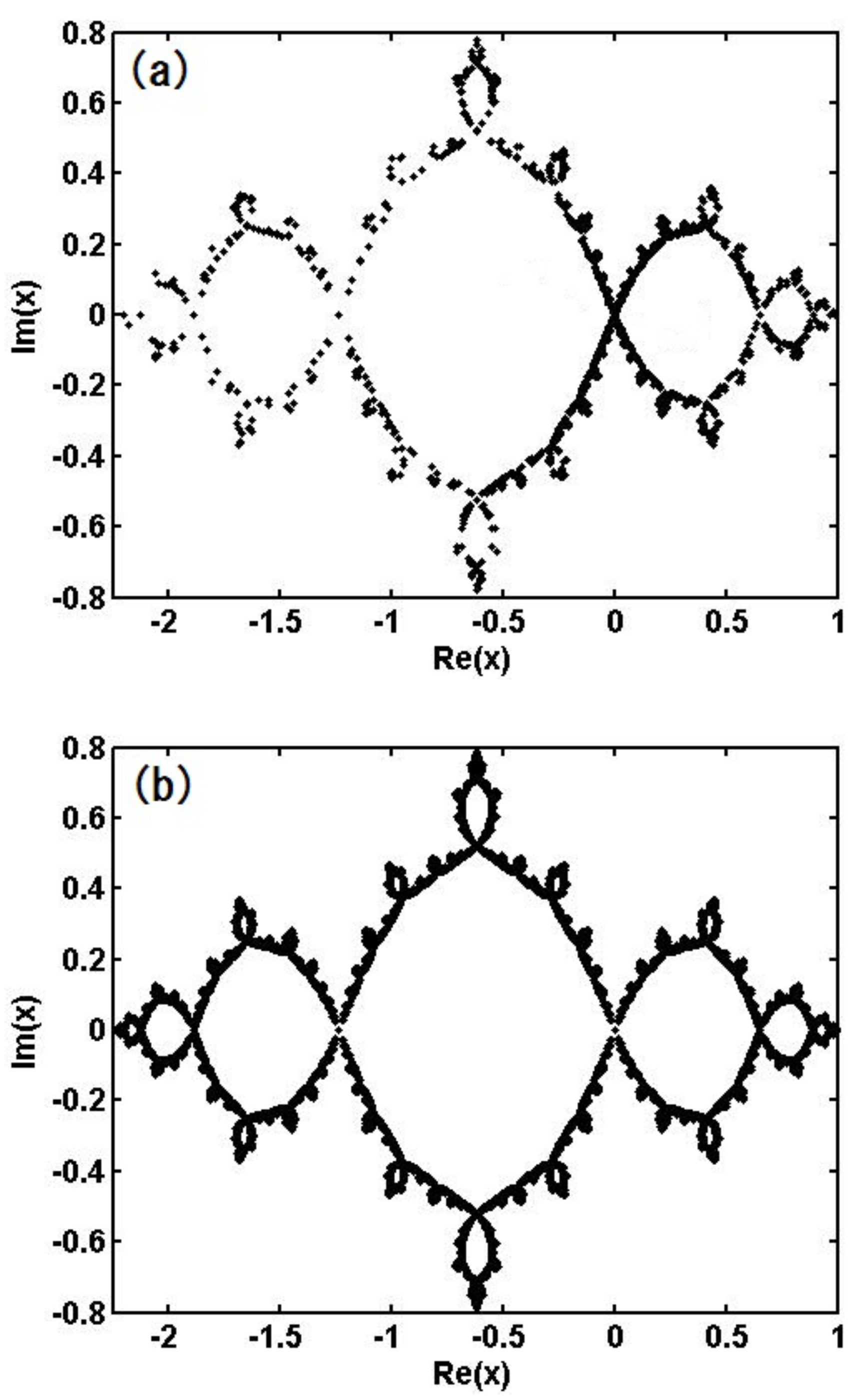
Figure 5 and Figure 6 (a) show the set of homoclinic points for $a=1.9408$ and $a=1.0$, respectively. These figures are calculated using the zeros of $x\left(t\right)$ obtained via the asymptotic expansion given in (5). In Figure 6 (a), the initial value of $t=t_r+i{t}_i$ (distant future) is selected as $27\le t_r\le 28$ and $t_i=3.0$. The number of obtained zeros $M_s=560$ (for the initial number of detecting points $K_0=2000$) at the acceleration after the final implementation of Newton’s method, where the typical initial values of $\left|x\right(t\left)\right|$ for the above time region are within the range ${10}^{100}-{10}^{5000}$ and the number of implementations of Newton’s method required for the convergence [$\left|x\left(t\right)\right|<O\left({10}^{-30}\right)$] is $12-20$ for almost all points; i.e., the convergence for $a=1.0$ is faster than that for $a=1.9408$.

In Figure 5 and Figure 6 (a), we retrieve the obtained values of t that provide $x\left(t\right)=0$ (the number of zeros; $M_s=1154$ for $a=1.9408$ and $M_s=560$ for $a=1.0$) to the past individually, as $t-1,t-2,t-3,\dots ,t-27$ (the value 27 is the initial value of $t_r$ that corresponds to distant future). We plot $(\Re [x(t-n)],\Im [x(t-n)\left]\right)$ (ℑ denotes the imaginary part) for all of these $t-n$ ($n=1,2,\dots 27$) together ($1154\times 27=31158$ points for $a=1.9408$ and $560\times 27=15120$ points for $a=1.0$ in all), where $t-27$ corresponds to the distant past. Thus, we obtain the set of homoclinic points. For $n=1-6$ and $n=25-27$, the value of $\left|x\right(t-n\left)\right|$ is very small and almost all points are located in the neighborhood of the fixed point $x=0$ for both $a=1.9408$ and $a=1.0$.

Figure 3. Results of Newton’s method and acceleration technique for $a=1.9408$ in the complex t plane, where the black points denote (a) the initial distribution, the distributions after (b) 5 and (c) 10 implementations of Newton’s method, and (d) the final distribution. The red points depict the “seeds" (the points satisfying $\left|x\right(t\left)\right|<100$) obtained by the acceleration after each implementations of Newton’s method. All seeds in (d) coincide with the zeros of $x\left(t\right)$ ($\left|x\left(t\right)\right|<{10}^{-30}$).

Figure 3. Results of Newton’s method and acceleration technique for $a=1.9408$ in the complex t plane, where the black points denote (a) the initial distribution, the distributions after (b) 5 and (c) 10 implementations of Newton’s method, and (d) the final distribution. The red points depict the “seeds" (the points satisfying $\left|x\right(t\left)\right|<100$) obtained by the acceleration after each implementations of Newton’s method. All seeds in (d) coincide with the zeros of $x\left(t\right)$ ($\left|x\left(t\right)\right|<{10}^{-30}$).

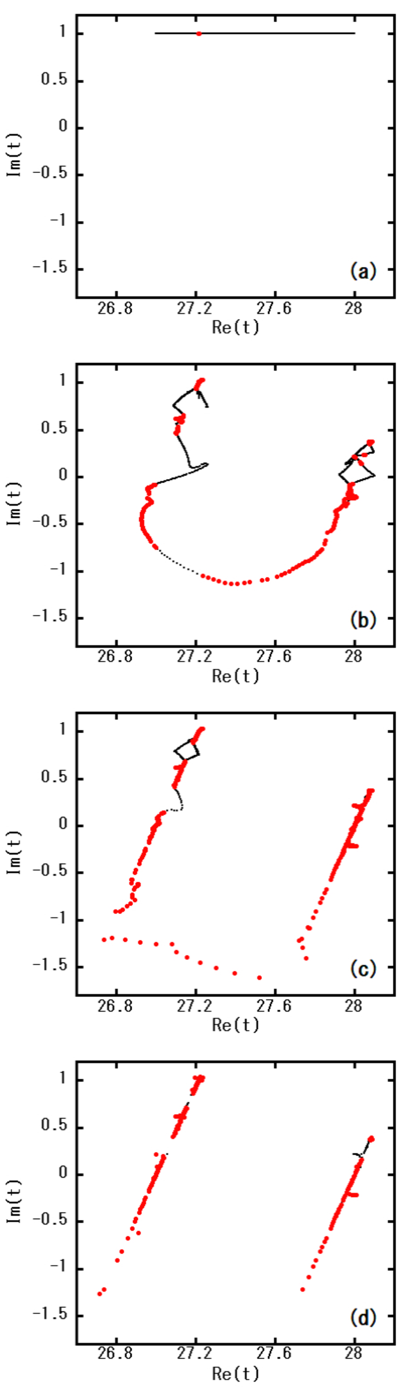
Figure 4. (a) Before and (b) after acceleration for the same number of implementations (four times) of Newton’s method, where the dynamical parameter a is the same as in Figure 3. The red points (seeds) have the same positions in (a) and (b).

Figure 4. (a) Before and (b) after acceleration for the same number of implementations (four times) of Newton’s method, where the dynamical parameter a is the same as in Figure 3. The red points (seeds) have the same positions in (a) and (b).

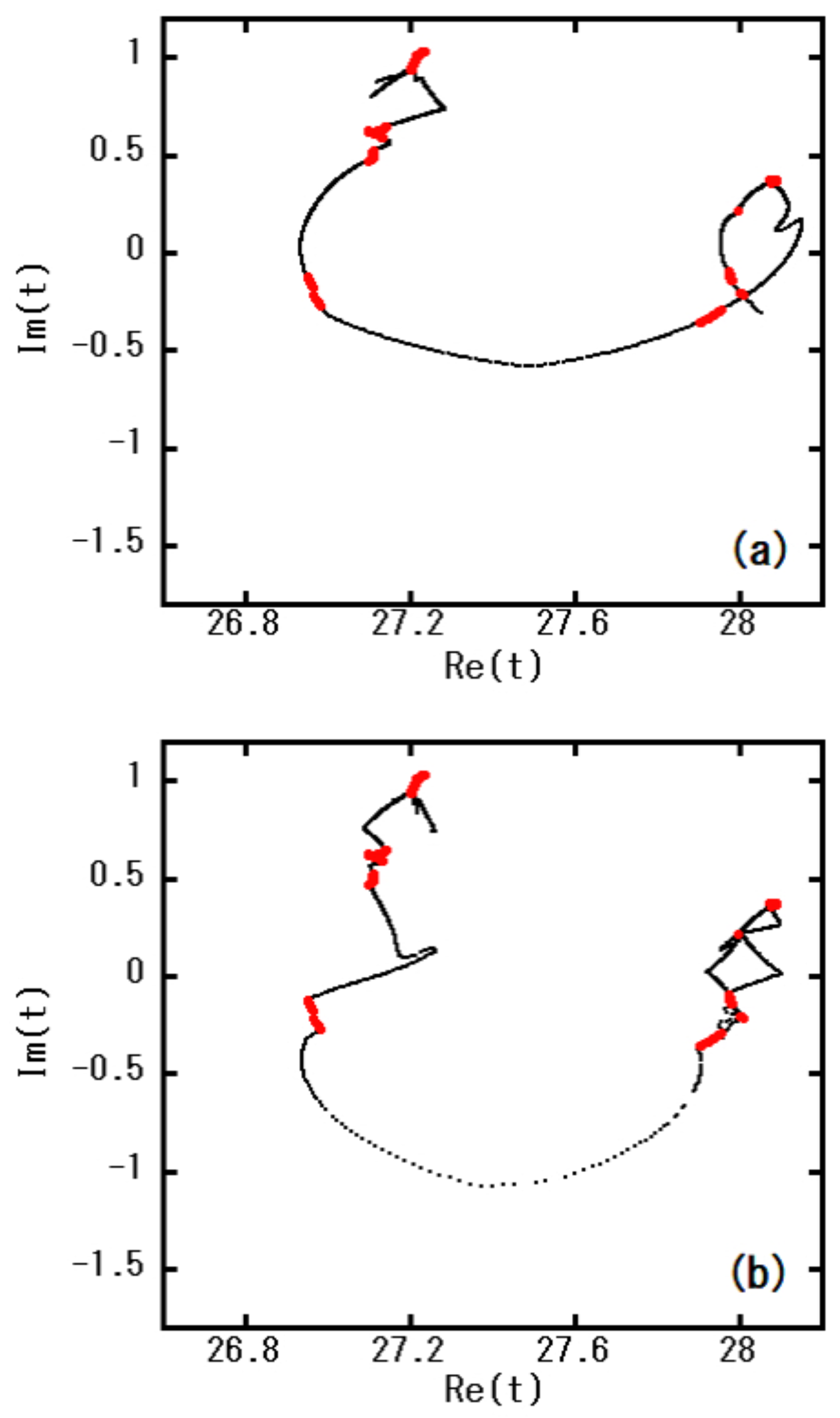
Figure 5 and Figure 6 (b) are the corresponding Julia sets calculated via the backward iteration of the quadratic map given in (3). Here, the backward iteration is given by

$$\begin{array}{c}\hfill x_{n+1}={\displaystyle \frac{-a{x}_f\pm \sqrt{a^2{x}_f^2-a{x}_n}}{a}}(n=0,1,2,\dots ),\end{array}$$

(17)

starting from the initial condition $x_0=0$ (fixed point), in which the calculation is performed with 64 digits and the number of iteration (i.e., the number of plotted points) is $2^{18}=262144$ for both Figure 5 and Figure 6.

Obviously, the figures (a) and (b) in Figs. Figure 5 and Figure 6 are identical, which guarantees the accuracy of our method. The set of homoclinic points has a fractal structure for both dynamical parameters $a=1.9408$ and $a=1.0$. As we see from Figure 2, the value $a=1.0$ in the map (3) belongs to the periodic region for $x\in \mathbb{R}$ and the chaotic behavior is not observed in the real space. However, the behavior of x in the complex plane is very complicated. This exhibits the essential complexity that the dynamical system (3) possesses.

It seems that the figures of Julia sets Figs. Figure 5 and Figure 6 (b) are more accurately than those depicted in Figure 5 and Figure 6 (a). However, we cannot extract any physically meaningful quantities from the backward iteration of map (3). On the other hand, each point in Figs. Figure 5 and Figure 6 (a) corresponds to a real physical event given by a deterministic function. The points included in the set of homoclinic points cannot escape and be physically meaningful, i.e., the observable events are all confined to this set. This result indicates that determination of the set of homoclinic points and identification of the orbit of each point allows every event from the past to the future to be determined; i.e., the dynamical systems given in Figure 5 and Figure 6 (a) are no longer chaotic but deterministic. The number of points that appear on the real axis increases as the dynamical parameter a becomes large, which is reflected in the complexity of the real dynamics, although the two sets of homoclinic points for $a=1.0$ and $1.9408$ have the same degree of complexity in the complex plane.

Figure 5. Homoclinic points for $a=1.9408$ obtained by using (a) the zeros of function $x\left(t\right)$ given by (5) and (b) the backward iteration of the original quadratic equation (17). The horizontal and vertical axes denote the real and imaginary parts of $x\left(t\right)$, respectively.

Figure 5. Homoclinic points for $a=1.9408$ obtained by using (a) the zeros of function $x\left(t\right)$ given by (5) and (b) the backward iteration of the original quadratic equation (17). The horizontal and vertical axes denote the real and imaginary parts of $x\left(t\right)$, respectively.

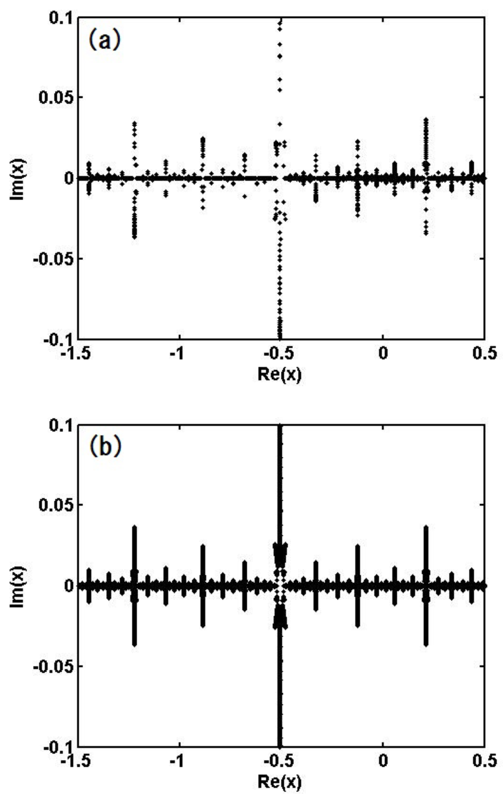
Figure 6. Homoclinic points for $a=1.0$ obtained by using (a) the zeros of function $x\left(t\right)$ and (b) the backward iteration (17).

Figure 6. Homoclinic points for $a=1.0$ obtained by using (a) the zeros of function $x\left(t\right)$ and (b) the backward iteration (17).

6. Concluding Remarks

We have succeeded in calculating the set of homoclinic points concretely, taking the quadratic map as an example. This enables us to capture the chaos deterministically. The obtained results coincide with those defined mathematically, which confirms the accuracy of our calculations. The set of homoclinic points provided in Figs. Figure 5 and Figure 6 involves numerical errors; however, our method itself is mathematically rigorous, and it is possible to decrease those errors through use of higher-performance computers or higher-precision computations. In the current study, we have calculated the set of homoclinic points in the region such that the dynamical system is uniformly hyperbolic. The convergence of the Newton’s method in the fully chaotic region without windows (e.g., the region of $a\ge 1.943$ in Figure 2) deteriorates significantly even if the acceleration scheme is applied. This fact suggests the existence of a lot of points of homoclinic tangency for the stable and unstable manifolds in the corresponding dynamical systems.

The method presented in this study is applicable to two-dimensional nonlinear dynamical systems such as Hénon maps and be used to determine the set of homoclinic points, provided the dynamical system is Laplace transformable. For the case that the stable and unstable manifolds are higher-dimensional (greater than one), the mathematical development is required.

References

- Poincare, H. Sur le probléme des trois corps et les équations de la dynamique. Acta Math. 1890, 13, 1–271.
- Alligood, K.T.; Sauer, T.D.; Yorke, J.A. Chaos. An introduction to dynamical systems.; Springer, New York, 1997.
- Devaney, R.L. An Introduction to Chaotic Dynamical Systems 2nd ed..; Westview Press, Boulder, Cololado, 2003.
- Mandelbrot, B. The fractal geometry of nature.; Freeman, New York, 1983.
- Birkhoff, G. Collected mathematical papers. 3 volumes; AMS, Providence, Rhode Island, 1950.
- Sinai, Y.G. Introduction to ergodic theory. Mathematical notes 18.; Princeton University Press, Princeton, New Jersey, 1975.
- Taub, A.H., Ed. Collected works of John von Neumann, 6 volumes.; Pergamon Press, Oxford, 1961–1963.
- Bowen, R. Equilibrium states and the ergodic theory of Anosov diffeomorphisms. Lecture notes in mathematics 470; Springer, New York, 1975.
- Ruelle, D. Thermodynamic formalism. Encyclopedia of mathematics and its applications, vol. 5.; Addison-Wesley, Boston, 1978.
- Smale, S. The mathematics of time, essays on dynamical systems, economic processes, and related topics.; Springer, New York, 1980.
- Barreira, L.; Pesin, Y.B. Lyapunov exponents and smooth ergodic theory. University lecture series vol. 23.; AMS, Providence, Rhode Island, 2002.
- Koda, R.; Hanada, Y.; Shudo, A. Ergodicity of complex dynamics and quantum tunneling in nonintegrable systems. Phys. Rev. E. 2023, 108, 054219. [CrossRef]
- Barahona, M.; Poon, C.S. Detection of nonlinear dynamics in short, noisy time series. Nature 1996, 381, 215–217. [CrossRef]
- Hamilton, J.D. Time series analysis.; Princeton University Press, Princeton, New Jersey, 1994.
- Guckenheimer, J.; Holms, P. Non-linear oscillations, dynamical systems, and bifurcations of vector fields.; Springer, New York, 1983.
- Lichtenberg, A.J.; Lieberman, M.A. Regular and Stochastic Motion.; Springer, New York, 1983.
- Tovbis, A. Asymptotics beyond all orders and analytic properties of inverse Laplace trnsforms of solutions. Commun. Math. Phys. 1994, 163, 245–255. [CrossRef]
- Gelfreich, V.; Sauzin, D. Borel summation and splitting of separatrices for the Hénon map. Ann. Inst. Fourier (Grenoble) 2001, 51, 513–567. [CrossRef]
- Écalle, J. Les fonctions résurgence, vol. 1.; Publ. Math. d’Orsay, Paris, 1981.
- Écalle, J. Les fonctions résurgence, vol. 2.; Publ. Math. d’Orsay, Paris, 1981.
- Écalle, J. Les fonctions résurgence, vol. 3.; Publ. Math. d’Orsay, Paris, 1985.
- Anastassiou, S.; Bountis, T.; Bäcker, A. Homoclinic points of 2D and 4D maps via the parametrization method. Nonlinearity 2017, 30, 3799–3820. [CrossRef]
- Poincare, H. Sur une classe nouvelle de transcendantes uniformes. Journ. de. Math. 1890, 6, 313–365.
- Blanchard, P. Complex analytic dynamics on the Riemann sphere. Bull. Amer. Math. Soc. 1984, 11, 85–141. [CrossRef]
- Fatou, P. Sur les équations fonctionnelles. Bull. Soc. Math. France 1919, 47, 161–271. [CrossRef]
- Fatou, P. Sur les équations fonctionnelles. Bull. Soc. Math. France 1920, 48, 33–94 and 208–314. [CrossRef]
- Julia, G. Memoire sur l’itération des fonctions rationnelles. J. Math. Pures Appl. 1918, 8, 47–245.
- Milnor, J. Dynamics in one complex variable, 3rd ed. Annals of mathematics studies 160.; Princeton University Press, Princeton, New Jersey, 2006.
- Cabré, X.; Fontich, E.; de la Llave, R. The parameterization method for invariant manifolds I. Manifolds associated to non-resonant subspaces. Indiana Univ. Math. J. 2003, 52, 283–328. [CrossRef]
- Cabré, X.; Fontich, E.; de la Llave, R. The parameterization method for invariant manifolds II. Regularity with respect to parameters. Indiana Univ. Math. J. 2003, 52, 329–360. [CrossRef]
- Cabré, X.; Fontich, E.; de la Llave, R. The parameterization method for invariant manifolds III. Overview and applications. J. Diff. Eqs. 2005, 218, 444–515. [CrossRef]
- Matsuoka, C.; Hiraide, K. Computation of entropy and Lyapunov exponent by a shift transform. Chaos 2015, 25, 103110. [CrossRef]
- Matsuoka, C.; Hiraide, K. Special functions created by Borel-Laplace transform of Hénon map. Electro. Res. Ann. Math. Sci. 2011, 18, 1–11. [CrossRef]
- Matsuoka, C.; Hiraide, K. Entropy estimation of the Hénon attractor. Chaos Solitons Fractals 2012, 45, 805–809.
- Widder, D.V. The Laplace transform.; Princeton University Press, Princeton, New Jersey, 1968.
- Atkinson, K.E. An introduction to Numerical Analysis, 2nd ed..; John Wiley & Sons, New Jersey, 1989.
- Yamamoto, T. Historical developments in convergence analysis for Newton’s and Newton-like methods. J. Comp. Appl. Math. 2000, 124, 1–23. [CrossRef]
Disclaimer/Publisher’s Note: The statements, opinions and data contained in all publications are solely those of the individual author(s) and contributor(s) and not of MDPI and/or the editor(s). MDPI and/or the editor(s) disclaim responsibility for any injury to people or property resulting from any ideas, methods, instructions or products referred to in the content. |
© 2025 by the authors. Licensee MDPI, Basel, Switzerland. This article is an open access article distributed under the terms and conditions of the Creative Commons Attribution (CC BY) license (http://creativecommons.org/licenses/by/4.0/).
Copyright: This open access article is published under a Creative Commons CC BY 4.0 license, which permit the free download, distribution, and reuse, provided that the author and preprint are cited in any reuse.