
Submitted:
29 December 2025
Posted:
30 December 2025
You are already at the latest version
Abstract
As Akasofu noted, no two geomagnetic storms are identical, yet the storm that occurred between November 12 and 14, 2025, stands out as an exceptional phenomenon. Its impact was evident across multiple layers of the ionosphere and numerous parameters, making it essential to conduct a comprehensive multi-parameter analysis of this event. Such an analysis relied upon data from the four LAERT topside sounders mounted aboard the recently-launched Ionosfera-M satellites. Global ionospheric dynamics was thoroughly examined during the storm period, particularly focusing on the polar and auroral zones, along with the equatorial anomaly region. Notable features included sharp electron density gradients, widespread F-layer disturbances, and the formation of giant plasma bubbles. These elements collectively contributed to the dynamic picture of the ionospheric storm captured through multi-parameter measurements by the LAERT sounders.
Keywords:
geomagnetic storm
; topside sounder
; auroral oval
; equatorial anomaly
1. Introduction
Despite extensive research into the ionospheric effects of geomagnetic storms over many years [1,2,3,4,5,6,7,8], these phenomena continue to be a focal point in ionospheric studies. Following the super geomagnetic storm of May 10-11, 2024 [9], the strong geomagnetic storm of November 11-14, 2025 is likely to become one of the most intensively studied events in the coming months. Unlike the study in [9], which utilized data from the SWARM satellite constellation, our work employes data from the “Ionozond” satellite constellation [10], comprising four Ionosfera-M satellites equipped with onboard topside sounders known as LAERT [11]. The capability of the LAERT topside sounder to deliver multi-parameter global monitoring of the ionosphere across four distinct local time sectors, while simultaneously measuring electron concentrations throughout the entire altitude range from 820 km down to the peak altitude of the F2 layer (hmF2), illustrates that the intensity of the so-called “fountain effect” does not necessarily correlate with geomagnetic storms. This conclusion stems from observations showing the formation of dual crests not just near hmF2 but also at the satellite's orbital altitude of 820 km under quiet geomagnetic conditions.
A comprehensive analysis of topside ionograms and dynamic HF spectra revealed detailed insights into the storm-induced dynamics of the high-, mid-, and low-latitude ionosphere, including the development of large-scale spread F regions and unusual plasma bubbles within the equatorial anomaly. The latitudinal migration of these crests has been visualized using vertical cross-section of the ionosphere, effectively illustrating their behavior across the full altitude range of the ionosphere.
The most impressive result is the registration of series of solar type III radio bursts simultaneously with the X5.1 solar flare at 10:04 UT on November, 11.
2. Main Characteristics of Geomagnetic Storm November 11-14
Between 11 and 14 November 2025, an active solar region (NOAA AR 14274) produced four solar flares and released four coronal mass ejections (CMEs), three of which were Earth-directed [12]. Two of the flares were of class X, and one that peaked at 10:04 UTC November 11 was of extreme energy class X5.1. Following this solar flare, a severe radio blackout was recorded across Europe, Africa, and Asia, lasting approximately from 30 minutes to one hour [13]. The extreme velocity of the last coronal mass plasma flow, reaching 1,500 km/s, allowed it to overtake and absorb the plasma of the previous ejections moving at a slower speed. Such storms are classified as cannibal coronal mass ejections. Half an hour after the X5.1 solar flare a rare phenomenon – a high-energy proton flux was registered by the ground based Aragats Solar Neutron Telescope (ASNT), a 77th Ground Level Enhancement (GLE) for the whole history of observing such events since 1944 [14].
This fascinating storm was chosen to investigate the impact on the ionosphere and to highkight the multi-parameter measurement capabilities of the LAERT topside sounder.
To correlate ionospheric variations with the storm development we will use the equatorial Dst index (Figure 1).
3. Experimental Setup and Methods
In this study, our primary data source consists of measurements acquired using the four topside sounders—LAERT instruments aboard the Ionosfera-M satellites. On July 25, 2025, the Ionozond satellite constellation was fully deployed with the successful launches of Ionosfera-M No. 3 and No. 4 spacecraft. These satellites operate in two mutually perpendicular, Sun-synchronous, near-circular orbits at an altitude of approximately 820 km. The equatorial crossing times for these orbits are 09:00–21:00 Local Time (LT) for the first pair and 03:00–15:00 LT for the second pair. The satellites of each pair are positioned in the opposite points of the orbit, 180° apart in latitude
The LAERT topside sounder supports nine distinct operational modes; however, for the purposes of this investigation, only two modes will be utilized: active vertical sounding and active spectrometry in relaxation sounding mode.
During vertical sounding, the sounder sweeps through a frequency range from 0.1 to 20 MHz across the 400 fixed frequencies. It uses step sizes of 25 kHz in the low-frequency band, 50 kHz in the mid-frequency band, and 100 kHz in the high-frequency band. The sounding cycle repeats every 10 s, resulting in 360 ionograms per hour with the spatial resolution of approximately 70 km along the orbit. The vertical resolution is 4.5 km.
To gather additional insights into the electromagnetic environment, the topside sounder records the levels of high-frequency emissions both prior to each sounding pulse and 2.5 ms afterward. This method allows distinguishing between natural emissions such as Auroral Kilometric Radiation (AKR), low-frequency emissions associated with precipitating electrons inside the auroral oval, and solar Type III radio bursts, as well as local plasma resonances induced by the sounding pulses at specific ionospheric plasma frequencies.
Through data processing, we track variations in key parameters including the critical frequency (foF2), local plasma frequency at the satellite altitude (fos) and peak height (hmF2) along the orbital path. These topside ionograms are subsequently converted into vertical profiles of electron density [16], which form the basis for reconstructing the global three-dimensional distributions of electron concentration [17,18].
The satellites in Sun-synchronous orbits are unable to monitor the diurnal variations of ionospheric parameters, which important for studying the dynamics of ionospheric storms at various stages. To address this issue, we utilized data from the Roshydromet's network of ground-based ionosondes located across the European longitude sector—Rostov-on-Don, Moscow, and Kaliningrad—as well as in the Far Eastern region—Khabarovsk, Magadan, and Petropavlovsk-Kamchatsky.
Combination of these technologies of monitoring the ionospheric parameters helped us to correctly interpret the ionospheric variations registered by satellites in different sectors of local time.
4. Results
Disturbances during geomagnetic storms affect all ionospheric layers from the D region to the upper ionosphere. The most prolonged changes are observed in the F2 layer of the ionosphere. That’s why we use for our analysis the variations of critical frequency foF2 at the height of the F-layer maximum hmF2.
4.1. Ground Based Measurements
To understand the dynamics of the ionosphere at high, middle and low latitudes during a storm, the distributions and variations of the critical frequency of the ionospheric F2 layer were examined in two longitudinal sectors – 20° - 40° E and 135°-160° E using the data of ground-based vertical sounding ionosondes mentioned above.
In the upper panel of Figure 3, the solid line represents the 27-day median of the foF2 parameter, while the dots indicate the critical frequency measurements taken at the Rostov-on-Don station. The observed ionospheric activity reveals an extended negative phase of the storm lasting from 0300 UT on November 12, 2025, until 0300 UT on November 13, 2025. During this period, the foF2 value dropped by 40% compared to its 27-day median. On November 13, 2025, there was a minor increase in the critical frequency noted later in the day. This pattern of ionospheric behavior was also typical for other stations within the same longitudinal sector, specifically Kaliningrad and Moscow.
In the bottom panel of Figure 3, analogous findings are presented for the Khabarovsk station. Here, however, the character of ionospheric variations differs significantly. At 0500 UT on November 12, concurrent with a pronounced decline in Dst index (as shown in Figure 1), a 20% rise in the ionospheric critical frequency was documented, marking the positive phase of the storm. Twenty hours later, the negative phase emerged, characterized by a 30% reduction in the critical frequency, persisting another nearly full day.
This distinctive ionospheric response mirrored one observed at other locations along the same longitudinal sector, namely Magadan and Petropavlovsk-Kamchatsky. By November 14th, recovery from the geomagnetic perturbation was evident throughout these regions.
These results demonstrate a non-uniform longitudinal response of the ionosphere to the geomagnetic storm. In the longitudinal sector of 20° - 40° E, where the onset of the geomagnetic storm occurred at the end of the night (0300 UT corresponds to 0600 LT), the ionospheric negative disturbance began synchronously with the geomagnetic disturbance. But in the case of the storm onset occurred during the day (135° - 160° E), when the D and E layers of the ionosphere were still present, a positive phase with an increase in concentration in the F layer was recorded. Only 20 hours later, by the end of the following night local time (2200 UT in the lower panel of Figure 3 corresponds to 0700 LT), ionosphere reacted with a decrease in the critical frequency. This result confirms the conclusions of [8] where dependence of the ionospheric reaction on the local time was studied with the GPS TEC measurements.
4.2. Topside Sounding Results
The topside ionospheric sounder installed on the Ionosphere-M spacecraft, operating on the same principles as ground-based ionosondes, makes it possible to track changes in the electron concentration over the entire latitude range. Because of the fact that the satellites have sun-synchronous orbits, the variations of the parameter values can be considered as a quasi-fixed longitude distribution (except the polar caps). The Figure 4 demonstrates the latitudinal distributions of the critical frequency along the daylight part of the satellite Ionosphere-M No. 3 orbit, which crossed the equator at ~15 LT. Figure 3 shows the critical frequency variations versus the geomagnetic latitude on November 11, 12, 13, and 14, in the time interval (05-06 UT) and in the longitudinal sector of 135°−160° E. The blue line demonstrates the reference distribution obtained on November 11, on the eve of the storm. The northern crest maximum of the equatorial anomaly (EA) is located at 16° N and is equal to 17.5 MHz, while the southern crest maximum is located at 18° S and cis equal to 16.5 MHz. The valley minimum between the crests is at 0° and is equal to 10 MHz.
The red curve was recorded at 05:06 UT on November 12, four hours after the storm's onset when the Dst index reached its minimum value. It shows a distinct poleward shift of the EA crests by approximately 10° in latitude. Notably, the southern EA crest has disappeared while the amplitude of the northern crest remains largely unchanged. This apparent northward displacement of a substantial layer characterized by elevated electron density likely resulted in an observable increase in the critical frequency compared to the median values throughout all day of November 12 across middle latitudes.
In contrast, the green curve corresponds to measurements taken at 05:06 UT on November 13, 2025. Herein, the critical frequency associated with the F2 layer peak at the northern EA crest had diminished by 1 MHz, and no discernible southern crest activity could be detected. Additionally, as evidenced by the critical frequency map derived from the SIMP ionospheric model [19] incorporating both terrestrial and space observation datasets (see Figure 5), the EA structure appears significantly compressed along longitudinal coordinates (upper panel of the Figure 5). Specifically, whereas prior to the storm event (as depicted in the upper panel of Figure 3) at local time 15:00 there is a sign of the active phase in the EA shape, then on the second day of the storm this moment is observable at the eastern boundary of the EA with one active crest (bottom panel of the Figure 5).
Note that the crests took their standard position on November 14 (black line, Figure 4).
To compare data from the ground-based ionosonde in Khabarovsk and the LAERT 3 topside sounder, upper panel of Figure 3 shows red circles corresponding to the topside sounding data as the satellite passed through a geomagnetic latitude of 50° in the longitudinal sector of 135°-160°. The patterns of the data are generally similar, but some longitudinal differences prevent a complete match.
It is interesting to follow up the variations of the local plasma frequency at the satellite altitude 830 km (Figure 6).
In quiet conditions, the distribution has a single maximum (Figure 6, blue line) above the geomagnetic equator, caused by the fountain effect. Four hours after the storm's onset, the plasma distribution pattern at an altitude of 830 km changes sharply. The magnetic field change and corresponding East directed electric field were so strong that it dramatically enhanced the fountain effect, with EA crests also appearing at an altitude of 830 km, with the latitudes of their maxima corresponding to the red curve in Figure 4. Plasma frequencies increased twofold across the entire latitude range outside the EA. This effect was no longer observed on November 13 and later.
As it was mentioned in Paragraph 2, the relaxation sounder mode give opportunity to observe the plasma resonances corresponding the principal frequencies of the ionospheric plasma (electron cyclotron frequency and its harmonics, local plasma and upper hybrid frequencies) as well as to obtain reflections from the ionospheric F-layer at altitude nearly 500 km. All these diagrams including the local plasma frequency are demonstrated at the dynamic spectra presented in the Figure 7.
As one can see the values of the upper hybrid frequency (second curve from the top in the Figure 7 (a-d) are very close to the local plasma frequency and are practically identical to those in the Figure 6 for corresponding times.
Reduction of the topside ionograms allows deriving the altitude profiles of the electron concentration from the satellite's altitude to the peak of electron density. The electron density at lower altitudes is using modeled altitude cross-sections. It is a method for reconstructing the total electron density profile based on the NeQuick model, proposed by Prof. S.M. Radicella (ICTP) and described in [20]. The architecture of the NeQuick model allows calculating the Ne(h) profile using the peak parameters and the thicknesses of the F2, F1, and E layers as reference values. In the general case [21], the foF2 and M3000F2 (or hmF2) values are specified by the coefficients of the CCIR (or URSI) model. The parameters of the maxima of the lower ionosphere are determined by simple empirical relationships based on the solar zenith angle and the level of solar activity. In our case, we use the values of foF2, hmF2, and the thickness of the upper part of the F2 layer (B2u), obtained from satellite ionograms, as initial parameters. The resulting latitudinal cross-sections, combining the results of Figure 3, Figure 4 and Figure 5, are shown in Figure 8.
4.3. Revealing the Longitudinal Differences in the Ionosphere Reaction on the Geomagnetic Storm
Let's examine the observation results in the 20° − 40° E longitudinal sector, where the onset of the geomagnetic storm occurred late in the night (3 UT corresponds to 6 LT). As noted above, the ground stations in this range responded with a decrease in the electron concentration from the first hours of the disturbance. We will also examine the results from the LAERT 3 topside sounder.
In Figure 9, the reference distribution obtained the day before the magnetic disturbance is shown by the blue line. A day later, the EA crests became less pronounced (Figure 7, red curve), and plasma frequencies across the entire range decreased almost twofold. The effect of the EA crest shift toward the poles is not observed. On November 13, an asymmetry in the ionospheric behavior is observed in the Southern and Northern hemispheres. In the northern hemisphere, plasma frequencies are higher than the reference values, which is also reflected in the ground-based ionosonde data (Figure 3, upper panel). In the Southern hemisphere, at mid-latitudes, the plasma frequency increased relative to the first day of the storm, but did not reach the reference values. The southern EA crest completely disappears similarly as was observed in the Far East. On November 14, the ionosphere is practically same as the reference value of November 11.
To compare data from the ground-based ionosonde in Rostov-on-Don and the LAERT 3 topside sounder, red circles are shown on the upper panel in Figure 3. These circles correspond to the topside sounder data as it passed over the geomagnetic latitude of 45° in the longitudinal sector of 20°-40°. The values of the critical frequency are generally consistent.
The results of the ionospheric plasma frequency (fps) measurements at the spacecraft altitude of 830 km are surprising (Figure 10). The observation results for November 11 were used as the reference fps distribution (blue line in Figure 10). On November 12, four hours after the onset of the geomagnetic storm, despite a drop in the foF2 critical frequency, the electron density in the upper ionosphere increased, with fps in the Northern hemisphere nearly doubling (red curve in Figure 10). However, 24 hours later, fps dropped sharply. In the Southern hemisphere and near the geomagnetic equator, it was 25% below the reference value, while in the Northern hemisphere, it was close to the reference value. By November 14, the effects of the storm were no longer visible.
4.4. Small Scale and Regional Storm Induced Irregularities
The storm-time variations in the ionosphere demonstrated in Figure 4 and Figure 10 and followed by detailed discussion are global in nature. The time scale is from several hours up to several days, and we see the global inflation and emptying of the ionosphere at different phases of the geomagnetic storm development.
Another very important factor typical to the effects of geomagnetic storm in the ionosphere is generation of local instabilities in the form of the irregular structures of different sizes as one can see in the right edge of Figure 7 b. Because of limited size of the paper, we provide only two examples of such formations: one in the polar region, and one in the equatorial ionosphere.
The chaotic variations of electron concentration mentioned above are presented in more details in the Figure 12.
In comparison with spectra presented in Figure 7 a,c,d for Northern hemisphere where the plasma frequency at altitude 500 km sis not exceed 2-3 MHz, in Figure 12 we see the rise of the plasma frequency till 7.5 MHz, but it is not the smooth line. From 06:49 till 06:54 we observe continuous negative drops of the plasma frequency more than two times up to 3 MHz similar to plasma bubbles in equatorial ionosphere. From both sides of this formation, we see the splashes of low frequency emission at f < 1 MHz which is generated by low energy electrons precipitating within the auroral oval. This irregular structure may be connected also with another factor: if to look at the local time and geomagnetic latitude we should accept the fact that the structure is within the cusp sector whish during the active phase of geomagnetic storm may contribute to the plasma irregularity formation.
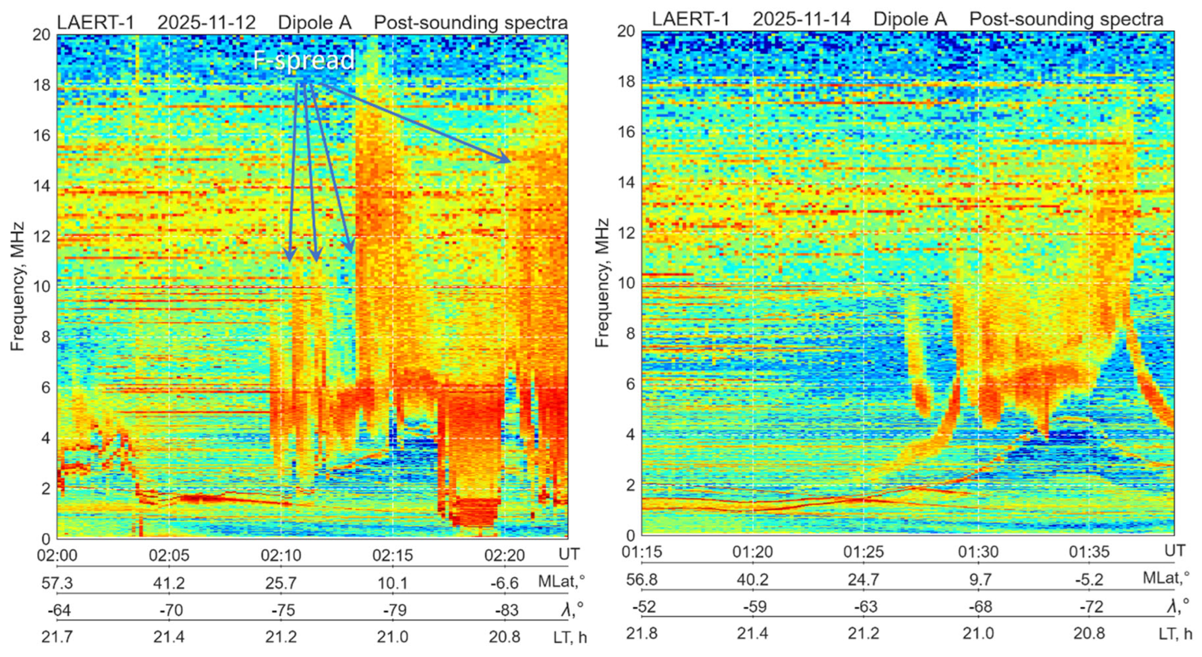
The second strong anomaly was observed in equatorial ionosphere nearly 21 LT when the post sunset reversal of the equatorial electric field causes the formation of equatorial anomaly [22]. Satellites Ionosfera-M No. 1 and No. 2 which orbit located just in this sector of local time register multiple plasma bubbles regularly [11], including the giant plasma bubbles. Formation of plasma bubbles is usually accompanied by the strong F-spread.
In the Figure 13 (left panel) is shown the extremely deep and giant in spatial extension (~1250 km) plasma bubble registered on 12 November 2025 between 02:15 and 02:20. We see the drop of plasma frequency from nearly 6.5 MHz up to 0.5 MHz what corresponds to the electron concentration drop from 5⋅105 sm-3 to 3⋅103 sm-3 i.e., more than 2 orders of magnitude. Such strong irregularities in the low latitudes create the serious problems for the radio communication and navigation [23].
In the right panel the similar pass of the satellite is shown but on 14 November after the geomagnetic storm relaxation. One can see only small plasma bubble nearly 10 s duration approximately on 01:33 on 14 November 2025.
5. Topside Sounder as an Astrophysical Device
The topside sounder working as a radiospectrometer is able to register not only signals generated in the ionosphere or penetrating from the ground industrial noises but also the signal from outside of the near earth space. We reported several cases of the solar type III bursts registered by the LAERT [11]. With the launch of the second pair of Ionosphere-M satellites there are cases when the same burst was registered by two satellites simultaneously when both of them were over the sunlit hemisphere. It is not simple to detect what event in the solar corona was the source of the registered burst and its identification has a special interest to reveal the physical mechanism of the burst’s generation. In this regard the simultaneous detection of a group of intense type III solar radio bursts by Ionosfera-M satellites No. 1 and No. 3 during an X5.1-class solar flare at 10:05 UT on November 11, 2025, has contributed to identifying one of the key indicators behind the subsequent geomagnetic storm discussed in this article.
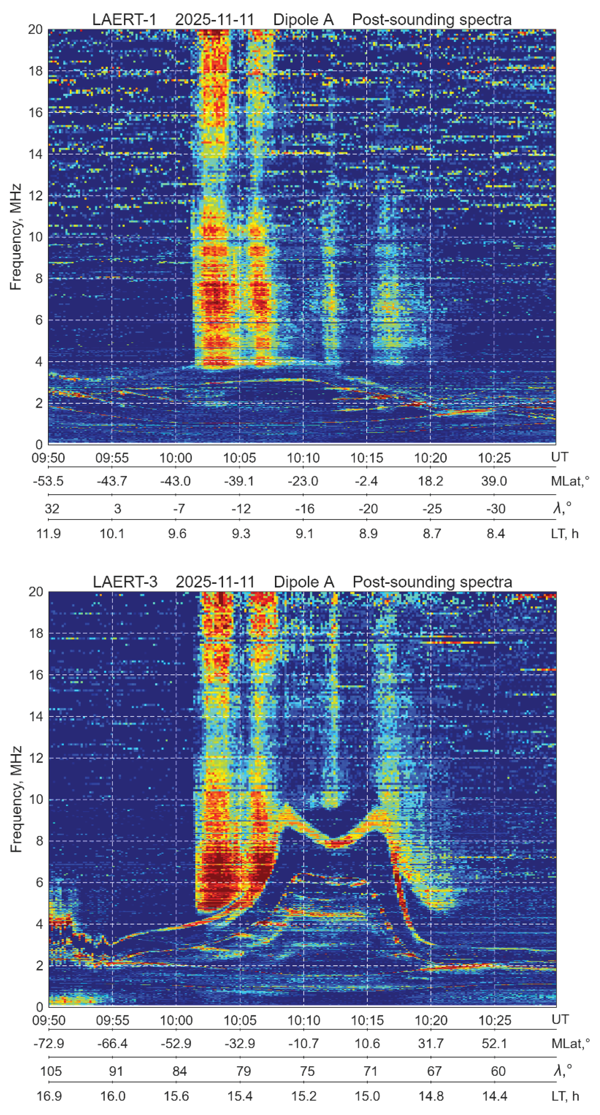
Figure 14.
Type III solar radio bursts registered by the Ionosphere-M No. 1 satellite (upper panel) and Ionosphere-M No.3 (lower panel) simultaneously with the X5.1 solar flare at 1005 UT 11 November 2025.
Figure 14.
Type III solar radio bursts registered by the Ionosphere-M No. 1 satellite (upper panel) and Ionosphere-M No.3 (lower panel) simultaneously with the X5.1 solar flare at 1005 UT 11 November 2025.
6. Discussion
This article presents a part of results obtained by the satellite constellation Ionozond during development of geomagnetic storm 11-14 November 2025. The complete collection of data for this storm requires more extended time including the data from other instruments registered the ionosphere parameters during this storm. Our intention was to demonstrate the wide opportunities of the satellite constellation especially the topside sounding technology and HF radiospectrometry. This is the first scientific study after the completion of flight tests and the commissioning of the system.
Comparison of satellite data with ground-based measurements showed their complete agreement and confirmed the presence of a longitudinal effect of a geomagnetic storm associated with the local time of onset of the main phase of a geomagnetic storm.
7. Conclusions
The revival of topside sounding technology [11] marks a new stage in the development of experimental methods for ionospheric research. New topside sounders offer significantly broader capabilities than previous generations of similar instruments. The combination of vertical sounding and high-frequency radiospectrometry allows for a more detailed study of the ionosphere's internal structure. We are only at the beginning of the application of these new instruments, which promises new, perhaps unexpected, results and discoveries.
Author Contributions
Conceptualization, methodology, investigation, writing—original draft preparation S.P; conceptualization; investigation, data curation, N.K.; investigation, data curation, visualization V.D.; software, visualization, writing—review and editing, K.Ts.
Funding
The work was carried out with the support of the Ministry of Science and Higher Education of the Russian Federation (theme/Monitoring, state registration No. 122042500031-8).
Data Availability Statement
Data are available on request.
Acknowledgments
For providing the geophysical indices data we acknowledge: WDC for Geomagnetism, Kyoto, Japan.
Conflicts of Interest
The authors do not have conflict of interest.
References
- Schuster, A., On the origin of magnetic storms. Proc. Roy. Soc. Lond. 1911. 85, 44–50.
- Chapman, S., and Ferraro, V. C. A., A new theory of magnetic storms. Terr. Mag. Atmos. Elect. 1933. 38, 79–96. [CrossRef]
- Akasofu, S.-I., and Chapman, S. The development of the main phase of magnetic storms. J. Geophys. Res. 1963. 68, 125–129. [CrossRef]
- Danilov, A.D. and Laštovička, J., Effects of geomagnetic storms on the ionosphere and atmosphere, Int. J. Geomagn. Aeron., 2002, 7, 278–286.
- Blagoveshchenskii, D.V., Effect of geomagnetic storms (substorms) on the ionosphere: 1. A review. Geomagn. Aeron. 2013. 53, 275–290 . [CrossRef]
- Akasofu S.-I. A Review of Studies of Geomagnetic Storms and Auroral/Magnetospheric Substorms Based on the Electric Current Approach. Front. Astron. Space Sci. 2021 7:604750. [CrossRef]
- Berényi K.A., Heilig B., Urbář J., Kouba D., Kis Á. and Barta V., Comprehensive analysis of the ionospheric response to the largest geomagnetic storms from solar cycle 24 over Europe. Front. Astron. Space Sci. 2023. 10:1092850. [CrossRef]
- Pulinets M.S., Budnikov P.A., Pulinets S.A., Global Ionospheric Response to Intense Variations of Solar and Geomagnetic Activity According to the Data of the GNSS Global Networks of Navigation Receivers, Geomagn. Aeron. 2023 63. 202–215 . [CrossRef]
- Nayak, C., Buchert, S., Yiğit, E., Ankita, M., Singh, S., Tulasi Ram, S., & Dimri, A. P. Topside low-latitude ionospheric response to the 10–11 May 2024 super geomagnetic storm as observed by Swarm: The strongest storm-time super-fountain during the Swarm era? Journal of Geophysical Research: Space Physics. 2025. 130, e2024JA033340. [CrossRef]
- Mogilevsky M.M., Chernyshov A.A., Pulinets S.A., Lukyanova R.Yu., Petrukovich A.A., Secrets of the Earth's ionosphere and the Ionosonde project for their disclosure, Zemlya i Vselennaya. 2025 No. 3, 5-23. [CrossRef]
- Pulinets S., Tsybulya K., Depuev V., Danilov I., Pulinets M., Ionospheric topside sounding revival, Advances in Space Research, 2026. 77, Issue 2, 2574-2587, . [CrossRef]
- Aerospace & Defence. Available online: https://www.aerospace-and-defence.com/esa-analyses-impacts-november-2025-solar-storm-3-cmes-earth-a-2234835b9110a63fc0c49764ea83ecbd/ (accessed on 20 12 2025).
- European Space Agency. Available online: https://www.esa.int/Space_Safety/Space_weather/Lessons_from_the_November_2025_solar_storm (accessed on 20 12 2025).
- Chilingarian A., Sargsyan B., Kozliner L., and Karapetyan T. Solar neutron and muon detection on November 11, 2025: First simultaneous recovery of energy spectra. arXiv:2512.07859 [astro-ph.SR] 2025 . [CrossRef]
- Data service. Available online: https://wdc.kugi.kyoto-u.ac.jp/aeasy/index.html (accessed on 21 12 2025).
- Jackson J.E. The Reduction of Topside Ionograms to Electron-Density Profiles, Proc. IEEE, 1969. 57, 960-976. [CrossRef]
- Depuev V.H., S.A. Pulinets. A global empirical model of the ionospheric topside electron density. Adv. Space Res., 2004. 34, 2016-2020.
- Pulinets S.A., Depuev V.H., Three-dimensional reconstruction of the global longitude irregularities in the ionosphere and their model representation. In Proceedings of the IRI Task Force Activity 2003, ICTP Publishing, IC/IR/2004/1, pp. 97-105.
- Lapshin, V.B.; Mikhailov, A.V.; Danilov, A.D.; Deminov, M.G.; Karpachev, A.T.; Shubin, V.N.; Mikhailov, V.V.; Tsybulia K.G.; Denisova V.N. The SIMP Model as a New State Standard for the Ionospheric Electron Density Distribution (GOST 25645.146). In Proceedings of the 25th All-Russian Conference on Radio Wave Propagation, Tomsk, Russian Federation, 03-09 July 2016 [in Russian].
- Nava, B.; Radicella, S.M.; Pulinets, S.; and Depuev, V. Modelling bottom and topside electron density and TEC with profile data from topside ionograms. Adv. Space Res. 2001, 27, 31–34. [CrossRef]
- Leitinger, R.; Zhang, M.-L.; Radicella, S. An improved bottomside for the ionospheric electron density model NeQuick. Ann. Geophys. It. 2005, 48, 525–534. [CrossRef]
- Li, J., Chen, Y., Liu, L., Le, H., Zhang, R., Huang, H., & Li, W. Occurrence of Ionospheric Equatorial Ionization Anomaly at 840 km height observed by the DMSP satellites at solar maximum dusk. Space Weather, 2021. 19, e2020SW002690. [CrossRef]
- L.M.M. Myint, N.Tongkasem, P. Supnithi, K. Hozumi, M. Nishioka. Equatorial Plasma Bubble (EPB) Observations at Low Latitude Regions of ASEAN. United Nations Workshop on the International Space Weather Initiative, Vienna, Austria 26 – 30 June 2023. https://www.unoosa.org/documents/pdf/psa/activities/2023/ISWI2023/presentations/ISWI2023_11_05.pdf.
- Kunitsyn V., Tereshchenko E. Ionospheric tomography. Springer-Verlag, Heidelberg, 2003. – 262 p.
Figure 1.
Equatorial Dst index for the period 10 – 15 November 2025.
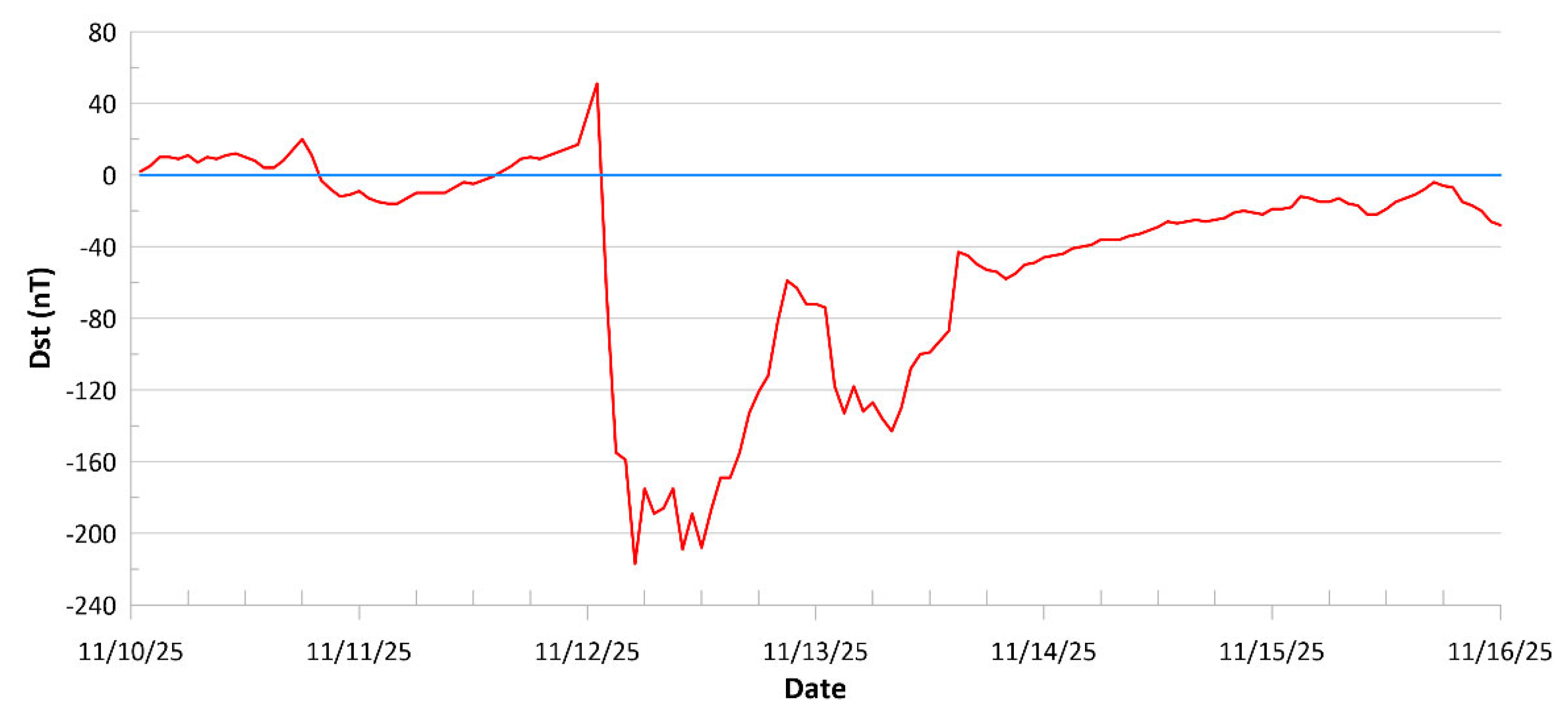
Figure 2.
From top to bottom AU, AL, ASY-D, ASY-H, SYM-H indices [15].
Figure 2.
From top to bottom AU, AL, ASY-D, ASY-H, SYM-H indices [15].
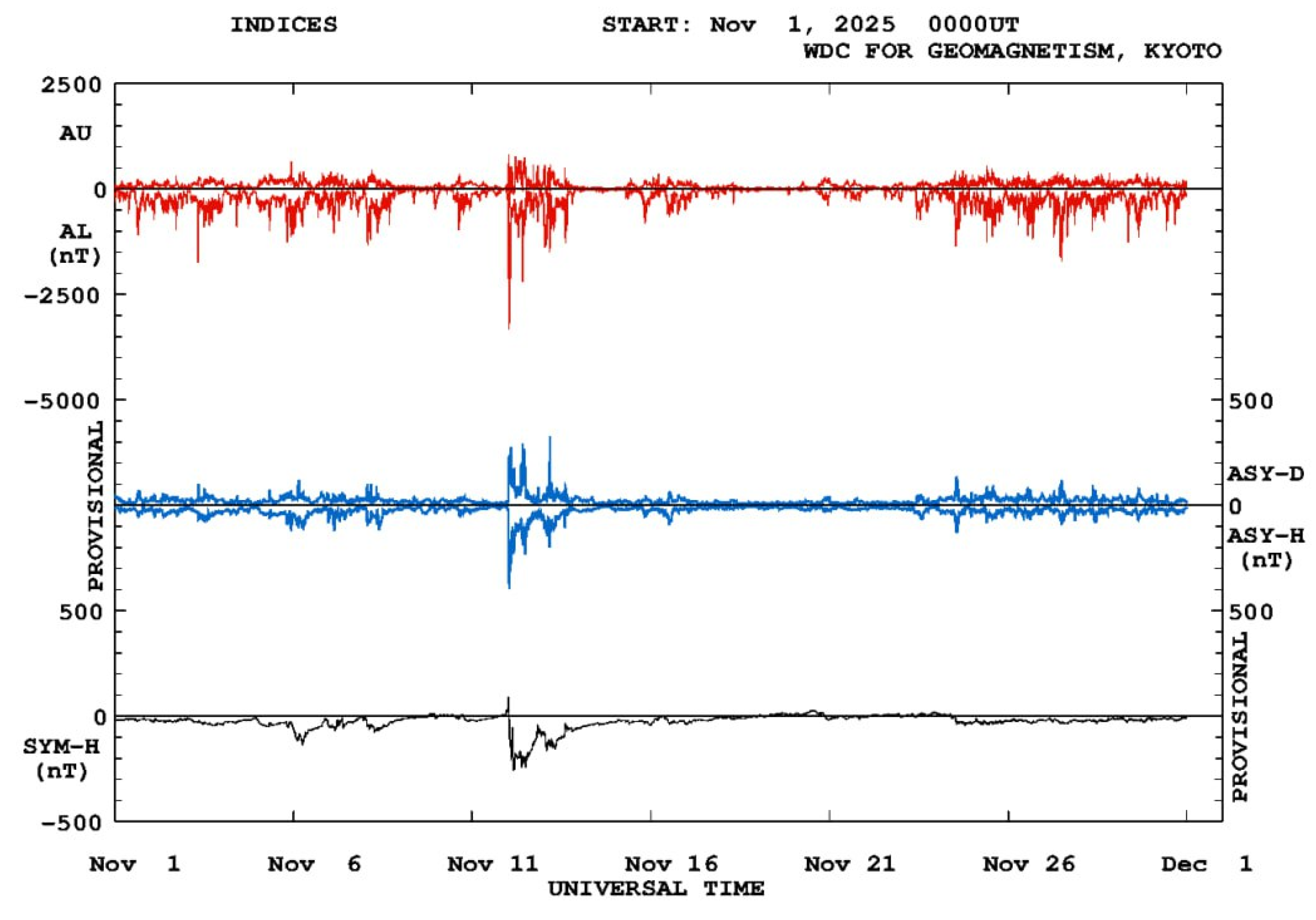
Figure 3.
Diurnal variations of foF2 on November 12–14, 2025. Upper panel –Rostov-on-Don station lower panel – Khabarovsk station. The solid line is the 27-day median, the dots are the observed values.
Figure 3.
Diurnal variations of foF2 on November 12–14, 2025. Upper panel –Rostov-on-Don station lower panel – Khabarovsk station. The solid line is the 27-day median, the dots are the observed values.
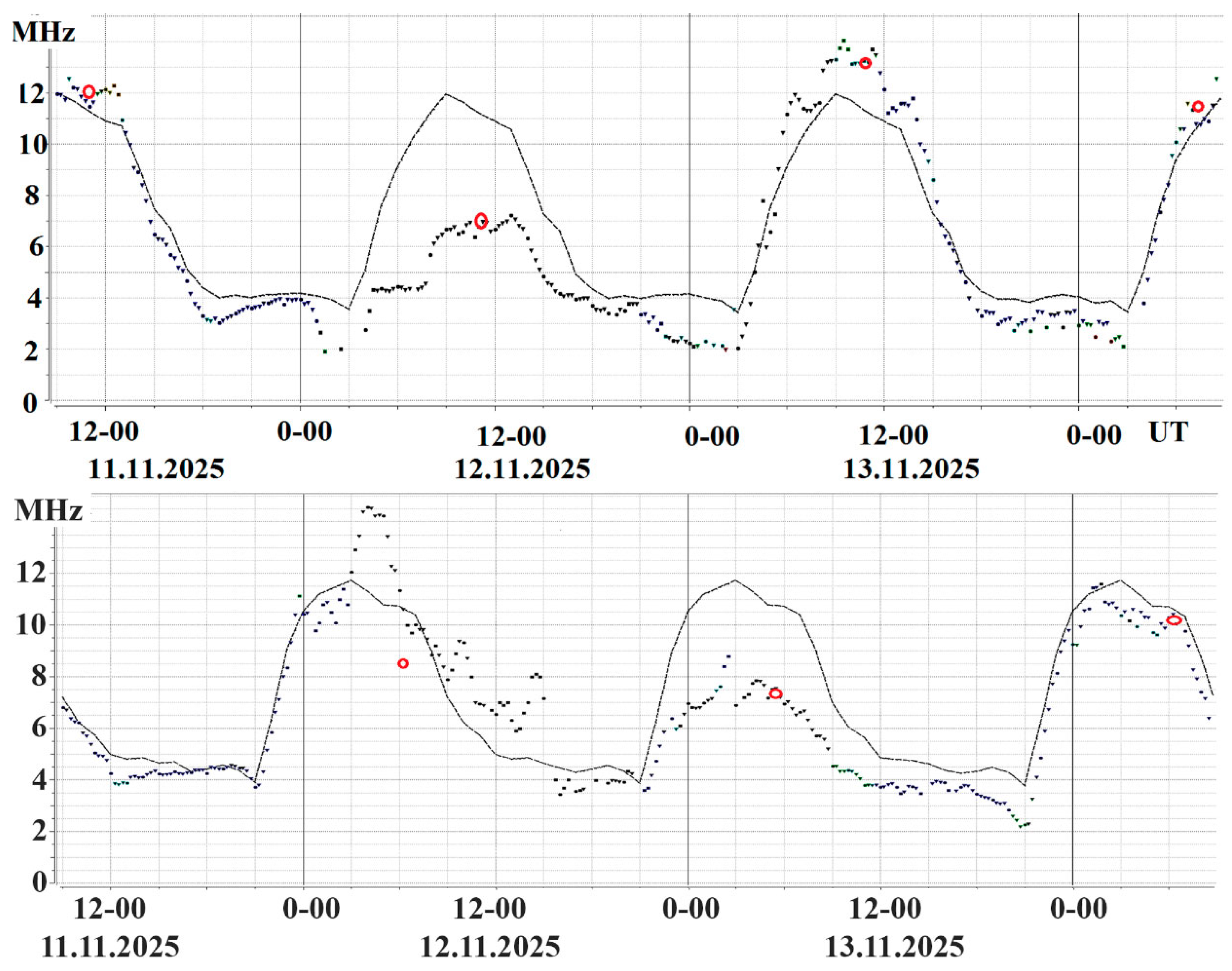
Figure 4.
Critical frequency variations in the ionosphere along the orbit of the Ionosfera-M No.3 spacecraft on November 11–14, 2025, at 5–6 UT in the longitudinal sector 135°–160° E.
Figure 4.
Critical frequency variations in the ionosphere along the orbit of the Ionosfera-M No.3 spacecraft on November 11–14, 2025, at 5–6 UT in the longitudinal sector 135°–160° E.
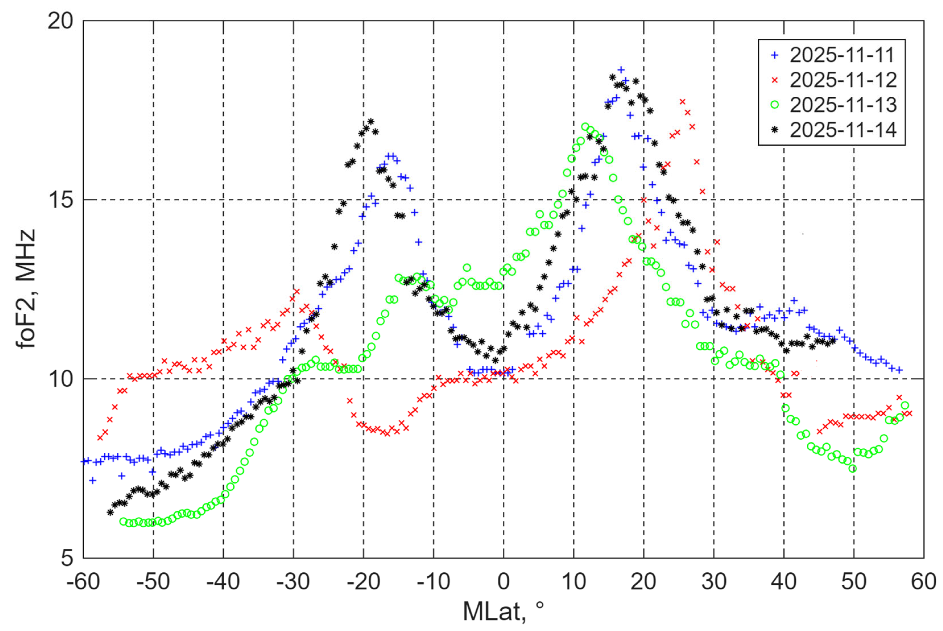
Figure 5.
Maps of the critical frequencies according to the SIMP model with assimilation of observation data from the Ionosphere-M spacecraft No. 1, 2, 3, 4. Upper panel –November 11 2025 0510UT, lower panel –November 13 2024 06:10 UT.
Figure 5.
Maps of the critical frequencies according to the SIMP model with assimilation of observation data from the Ionosphere-M spacecraft No. 1, 2, 3, 4. Upper panel –November 11 2025 0510UT, lower panel –November 13 2024 06:10 UT.
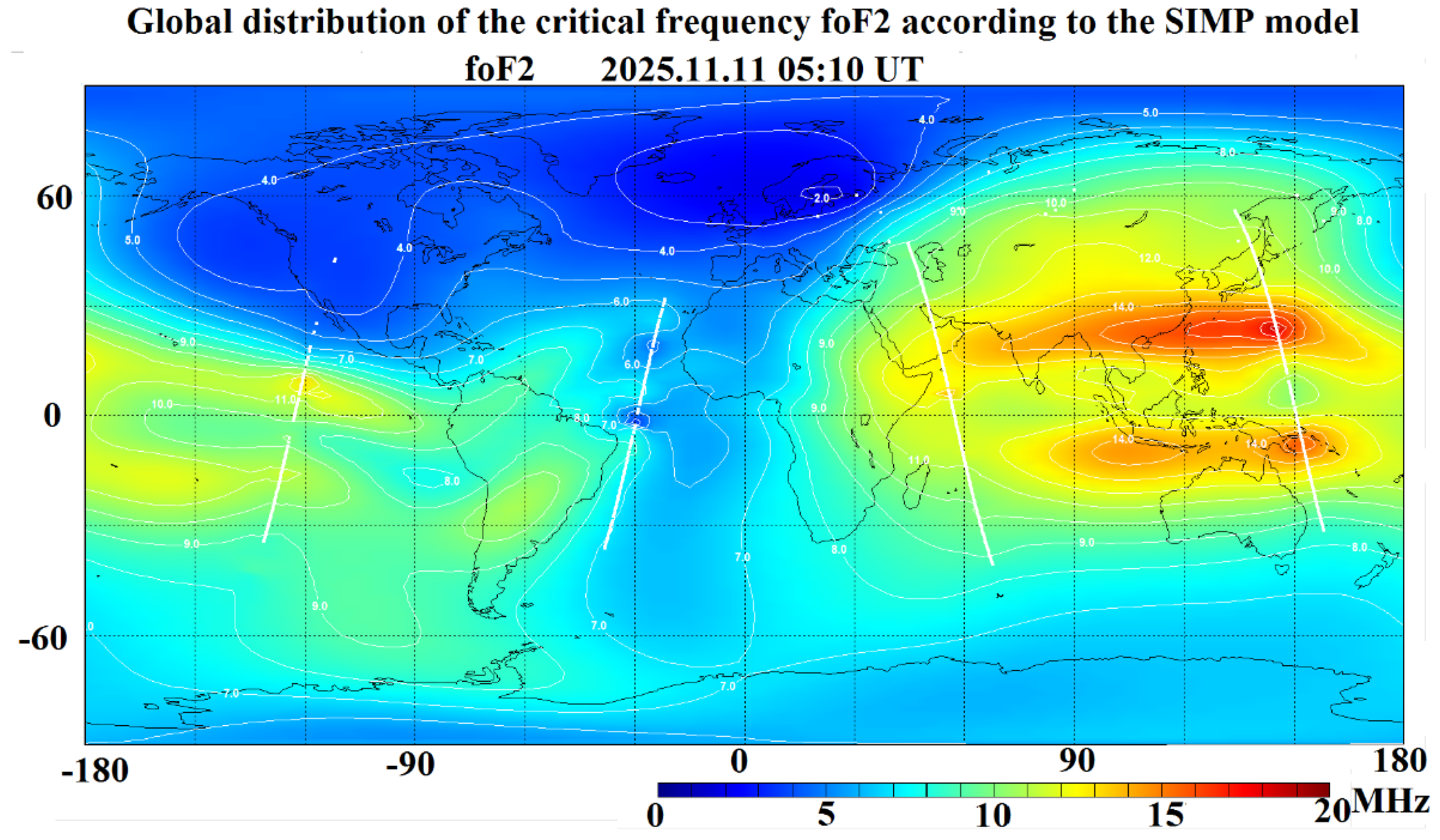
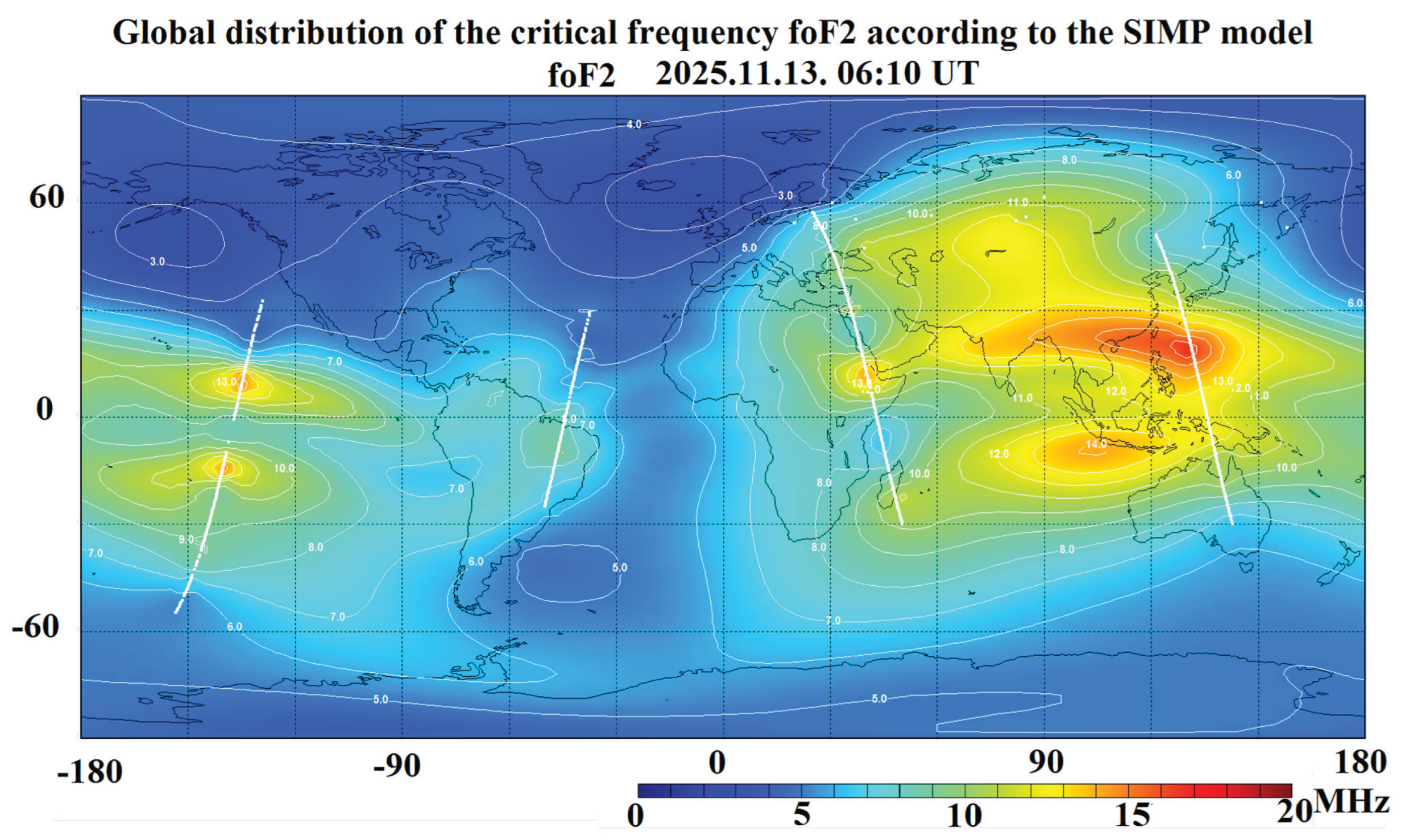
Figure 6.
Distributions of plasma frequencies along the orbit of the Ionosphere-M No. 3 spacecraft at the altitude of the spacecraft on November 11–14, 2025, at 5–6 UT in the longitudinal sector 135°–160° E.
Figure 6.
Distributions of plasma frequencies along the orbit of the Ionosphere-M No. 3 spacecraft at the altitude of the spacecraft on November 11–14, 2025, at 5–6 UT in the longitudinal sector 135°–160° E.
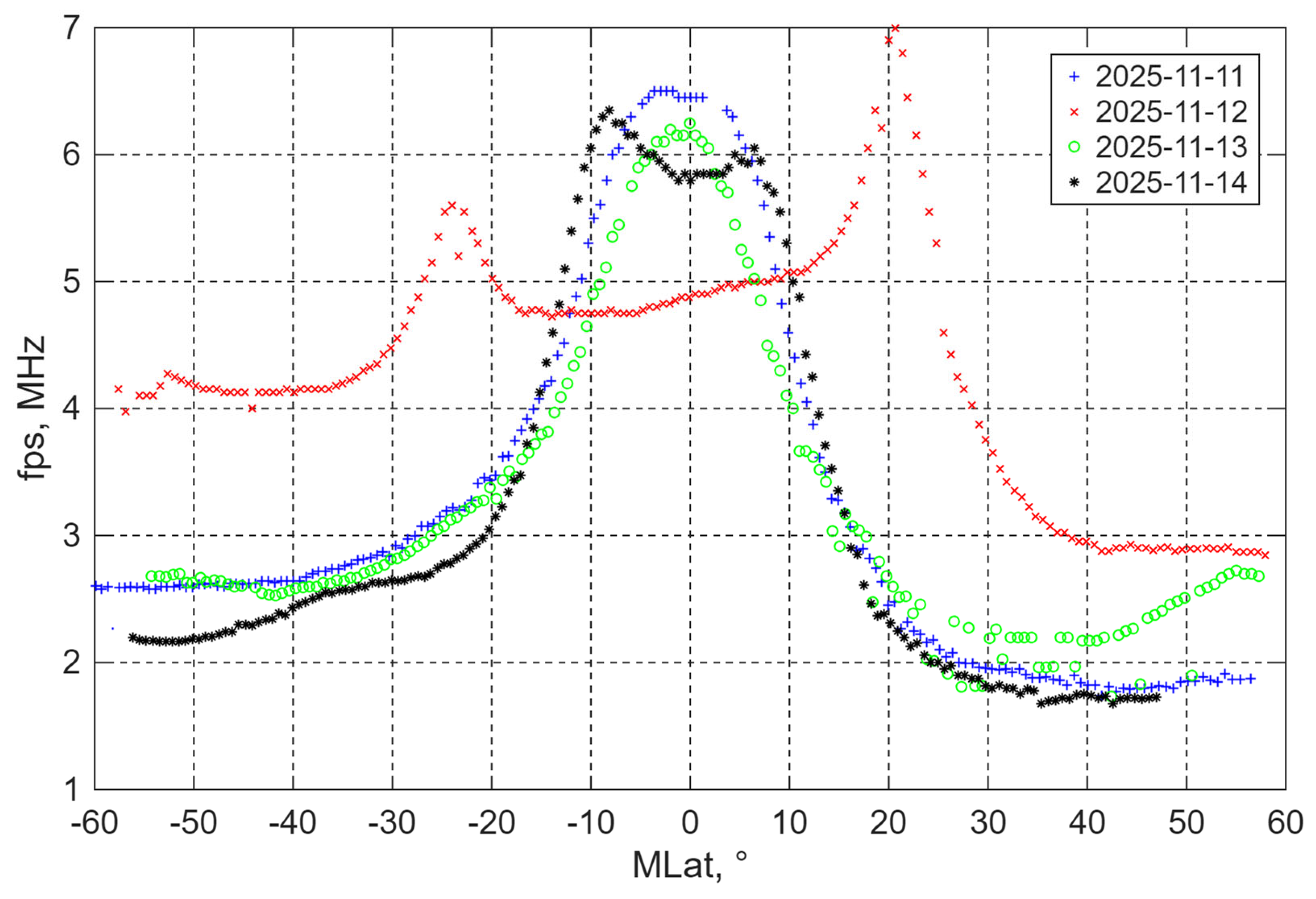
Figure 7.
Dynamic spectra obtained by the satellite Ionosfera-M No. 3 passes. Time periods are the same as those demonstrated in the Figure 6 depicting the variations of the local plasma frequency.
Figure 7.
Dynamic spectra obtained by the satellite Ionosfera-M No. 3 passes. Time periods are the same as those demonstrated in the Figure 6 depicting the variations of the local plasma frequency.
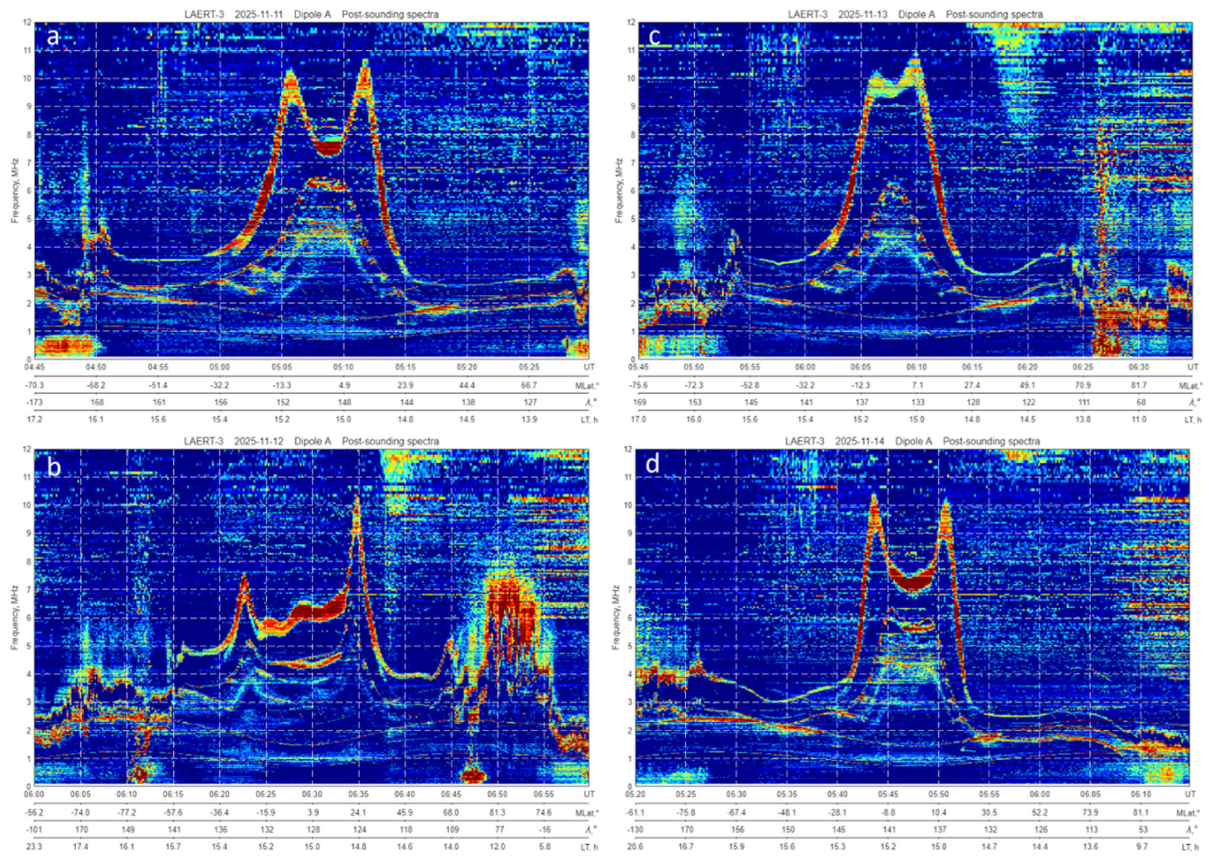
Figure 8.
Tomographic reconstruction of the EA dynamics during the geomagnetic storm 11-14 November 2025 within the longitudinal sector 135°–160° E.
Figure 8.
Tomographic reconstruction of the EA dynamics during the geomagnetic storm 11-14 November 2025 within the longitudinal sector 135°–160° E.
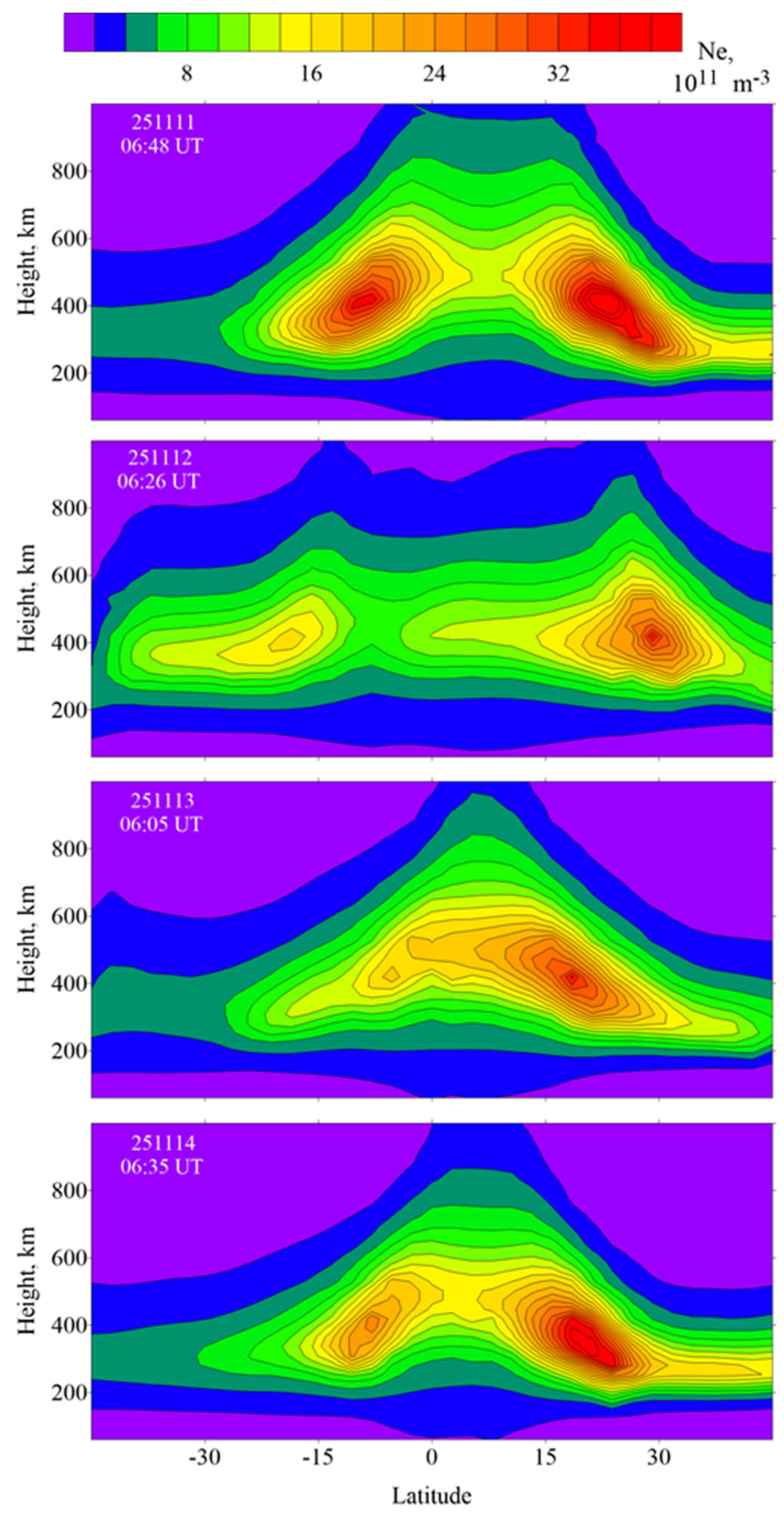
Figure 9.
Critical frequency distributions versus the geomagnetic latitude along the spacecraft orbits on November 11–14, 2025, at 11–12 UT in the longitudinal sector 20°–40° E.
Figure 9.
Critical frequency distributions versus the geomagnetic latitude along the spacecraft orbits on November 11–14, 2025, at 11–12 UT in the longitudinal sector 20°–40° E.
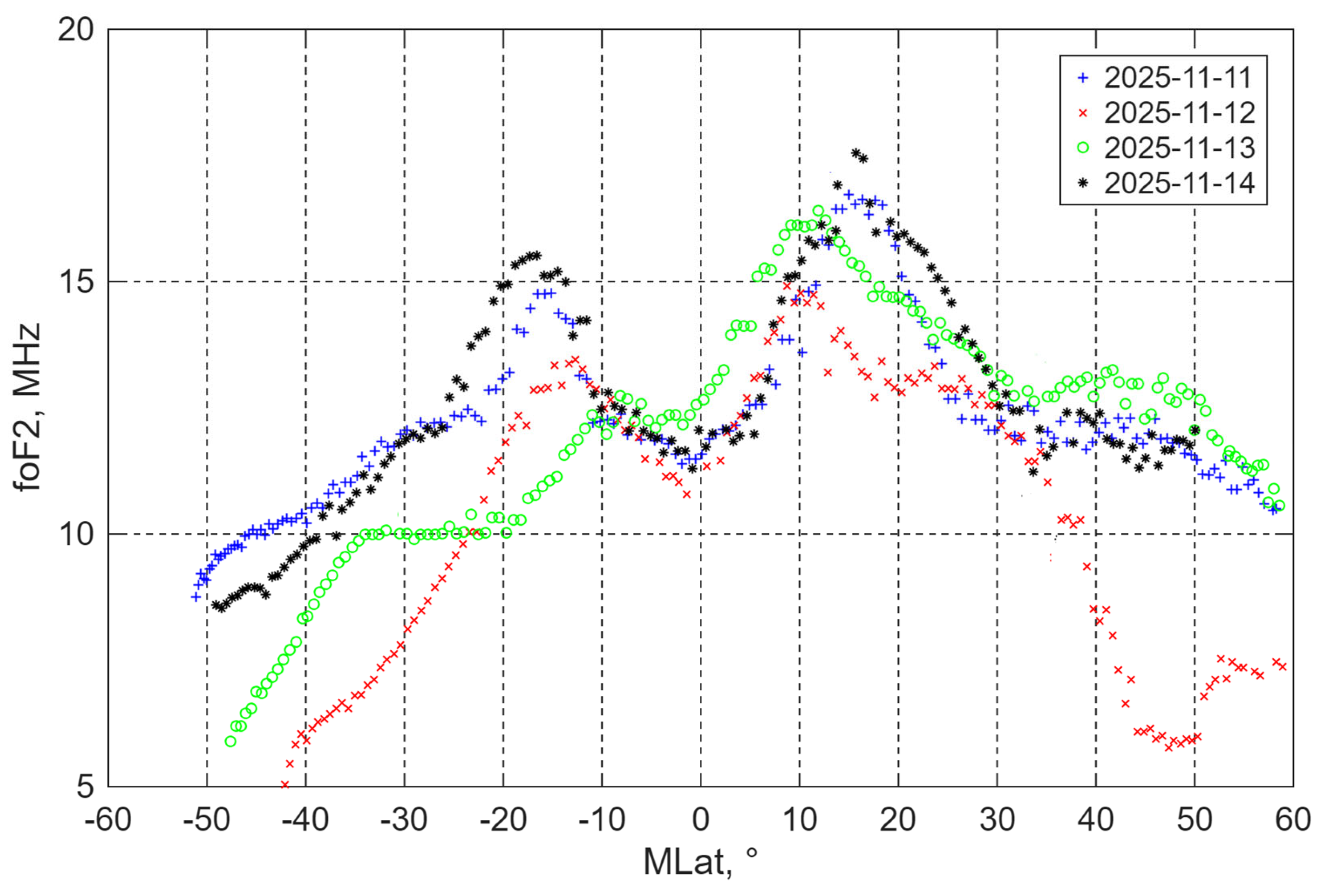
Figure 10.
Distributions of plasma frequencies along the orbit of the Ionosphere-M No. 3 spacecraft at the altitude of the spacecraft on November 11–14, 2025, at 11–12 UT in the longitudinal sector of 20°–40° E.
Figure 10.
Distributions of plasma frequencies along the orbit of the Ionosphere-M No. 3 spacecraft at the altitude of the spacecraft on November 11–14, 2025, at 11–12 UT in the longitudinal sector of 20°–40° E.
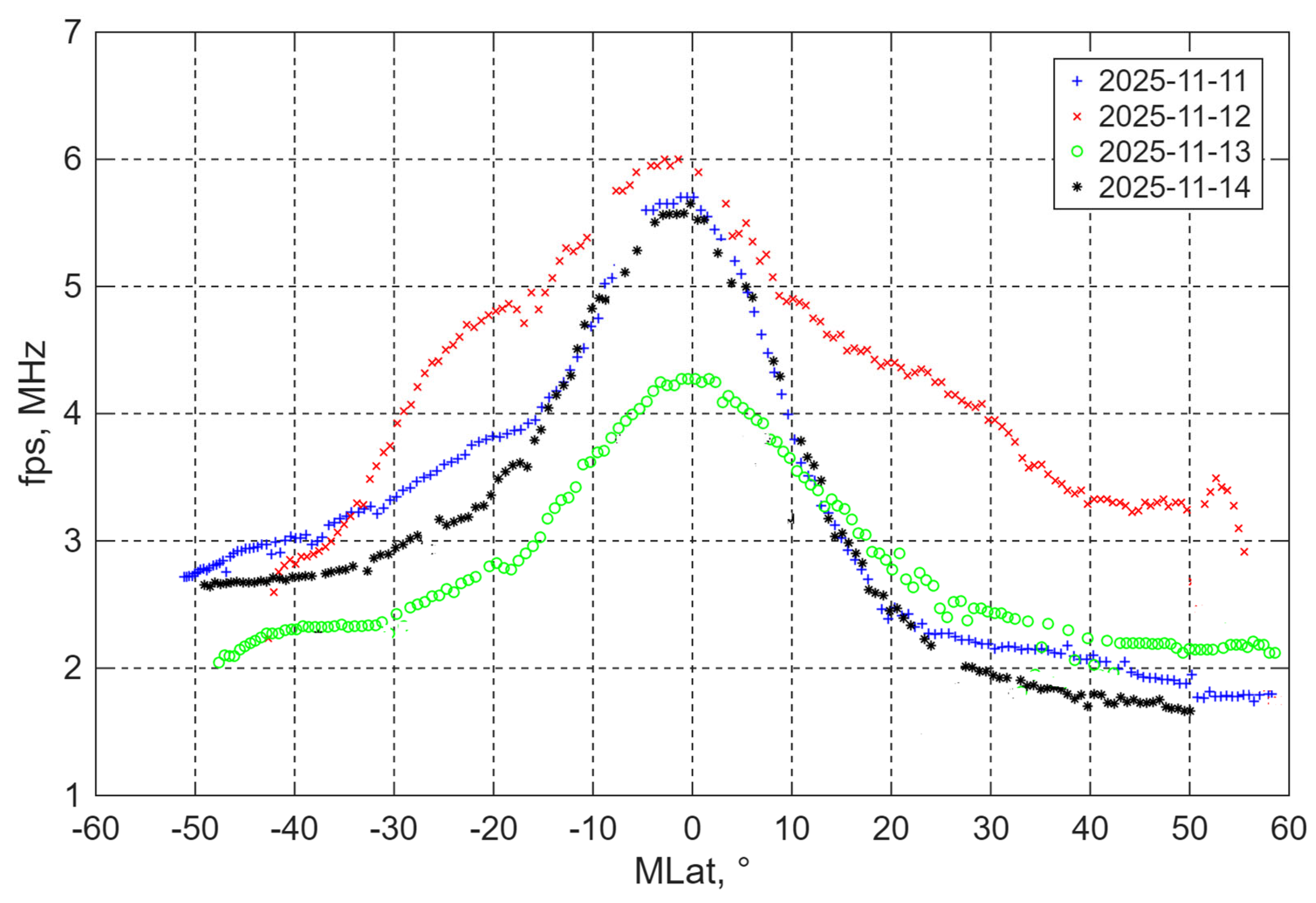
Figure 11.
Dynamic spectra corresponding to the satellite Ionosfera-M No. 3 passes demonstrated in the Figure 9 and depicting variations of the local plasma frequency.
Figure 11.
Dynamic spectra corresponding to the satellite Ionosfera-M No. 3 passes demonstrated in the Figure 9 and depicting variations of the local plasma frequency.
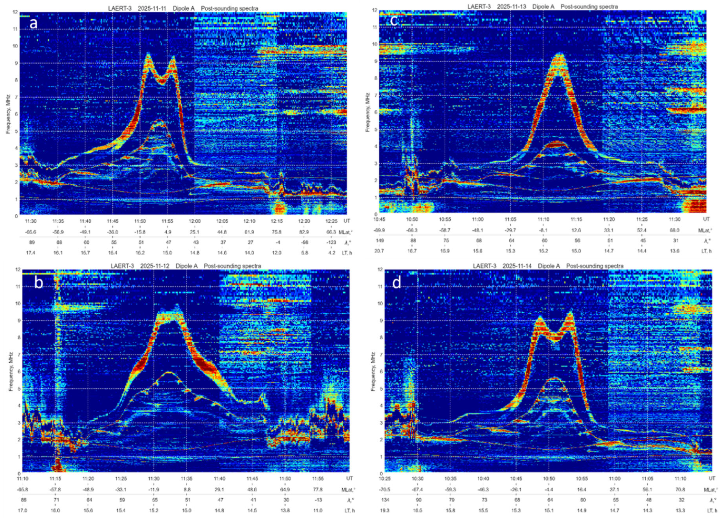
Figure 12.
Dynamic relaxation spectrum over the North polar ionosphere at 06:40 – 07:10 UT 12 November 2025.
Figure 12.
Dynamic relaxation spectrum over the North polar ionosphere at 06:40 – 07:10 UT 12 November 2025.
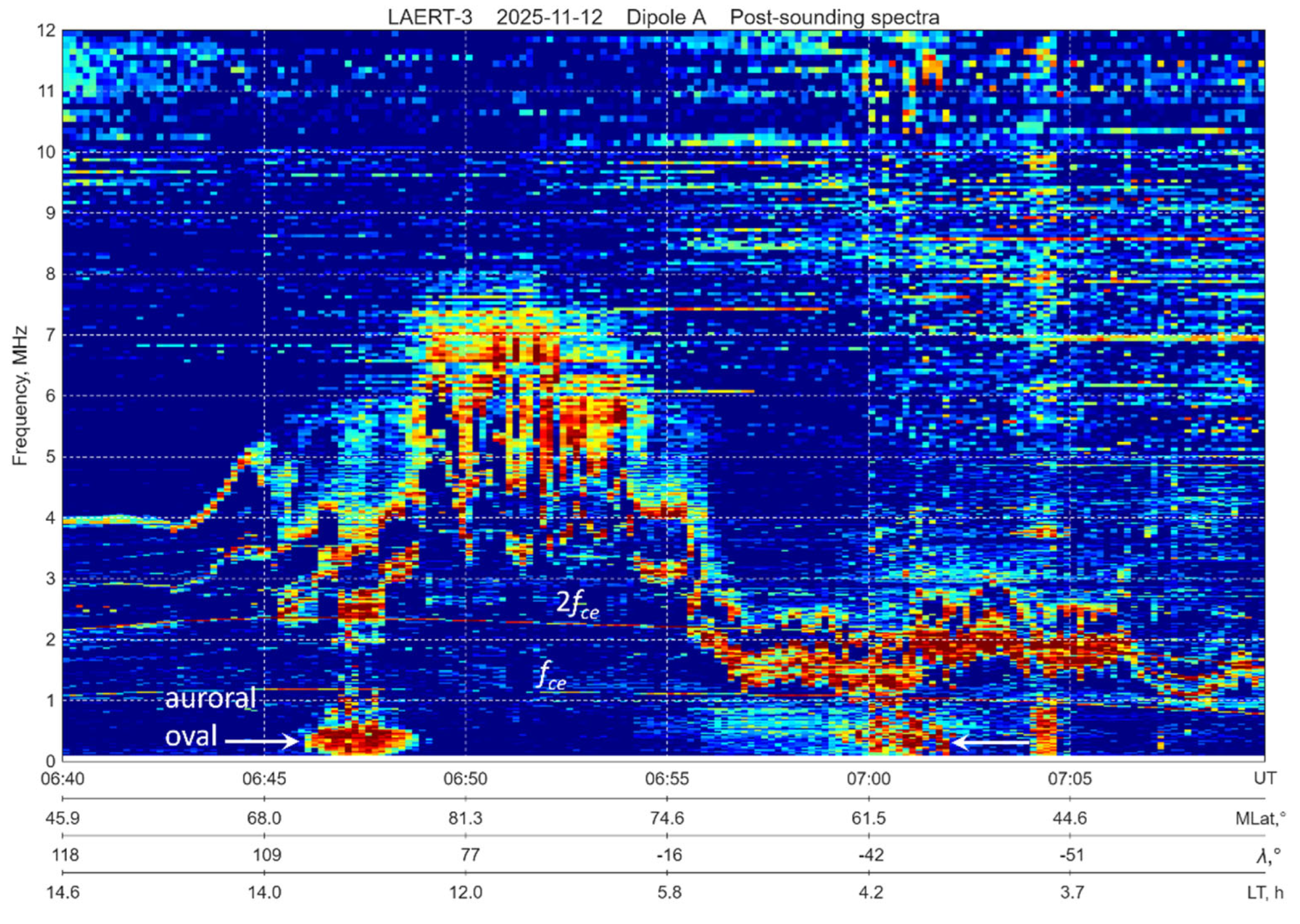
Figure 13.
Left panel – dynamic relaxation spectrum collected at 02:00 – 02:25 UT on 12 November 2025. Right panel – dynamic relaxation spectrum collected at 01:15 – 01:40 UT on 14 November 2025.
Figure 13.
Left panel – dynamic relaxation spectrum collected at 02:00 – 02:25 UT on 12 November 2025. Right panel – dynamic relaxation spectrum collected at 01:15 – 01:40 UT on 14 November 2025.
Disclaimer/Publisher’s Note: The statements, opinions and data contained in all publications are solely those of the individual author(s) and contributor(s) and not of MDPI and/or the editor(s). MDPI and/or the editor(s) disclaim responsibility for any injury to people or property resulting from any ideas, methods, instructions or products referred to in the content. |
© 2025 by the authors. Licensee MDPI, Basel, Switzerland. This article is an open access article distributed under the terms and conditions of the Creative Commons Attribution (CC BY) license (http://creativecommons.org/licenses/by/4.0/).
Copyright: This open access article is published under a Creative Commons CC BY 4.0 license, which permit the free download, distribution, and reuse, provided that the author and preprint are cited in any reuse.


