
Submitted:
28 December 2025
Posted:
29 December 2025
You are already at the latest version
Abstract
This study explores the use of machine learning to predict high-cycle fatigue (HCF) be-havior and fatigue crack growth rate (FCGR) in Co-Cr-Mo alloys manufactured through laser powder bed fusion. Two machine learning (ML) models: extreme gradient boosting (XGB) and deep neural networks (DNN), are implemented to estimate HCF and FCGR across three distinct scanning strategies. The raw datasets for HCF and FCGR are taken from previously performed experiments. The HCF dataset is augmented using a Gaussian Mixture Model, while the FCGR dataset is used in its raw form. Following hyperparameter optimization, both models exhibited quite similar accuracy on validation datasets. Their performance was assessed during testing using mean squared error (MSE) and R2 scores. The XGB model demonstrated higher accuracy in HCF predictions by achieving higher R2 scores. In contrast, the DNN model performed better in FCGR predictions and yielded higher R2 scores compared to XGB. The good agreement with the experimental dataset shows that these two ML techniques are effective in predicting HCF and FCGR behavior.
Keywords:
machine learning
; XGB
; DNN
; scanning strategy
; Co-Cr-Mo alloy
; fatigue
1. Introduction
Mostly, the key components of bio-implants [1,2] and aerospace structures [3] have intricate shapes that undergo complex repeated loadings. These loadings result in fatigue damage, which combines with environmental factors and leads to premature failures. Therefore, a complete fatigue understanding is an important aspect in the material design process. Recently, additively fabricated Co-Cr-Mo alloy has garnered notable attention across several sectors due to its exceptional combination of mechanical properties [2], corrosion resistance [3], biocompatibility [4], wear resistance [5] and admirable strength-to-weight ratio for lightweight lattice structures [6]. The fatigue behavior of additively fabricated components/parts depends on various process parameters, including build orientation [7,8], layer thickness, scanning strategy [9], scanning speed [10], and many more.
Conventional methods of fatigue assessment depend on extensive, time-consuming, and costly experiments, yet their ability to generalize is limited by the experimental ranges. To overcome this limitation, numerous numerical predictive methods (such as S-N curve-based models, Paris law model, probabilistic fatigue approaches, and machine learning based techniques) have emerged that eliminate the need for these labor-intensive experiments. Among these methods, machine learning (ML) is a viable solution [11,12]. ML is recognized by the scientific community very quickly due to its ability to analyze complex relationships between variables and make predictions. Various regression models can be incorporated into ML, such as XGBoost (XGB) [13], Support Vector Regression (SVR) [14], k-nearest neighbor algorithm (KNN) [15] and Deep Neural Networks (DNN) [16]. These methods have specific advantages: XGB utilizes greedy algorithms and parallel processing to enhance training and prediction speeds [17], SVR exhibits strong generalization ability on small datasets and excellent robustness to overfitting [18], KNN is particularly useful when there is little or no prior knowledge about the distribution of the data [19], and DNN are feasible for application to both small dataset [20] as well as large dataset [21]. ML is a powerful tool for modelling vast amounts of data without relying on physical mechanisms. ML-based data mining techniques have been widely applied in fatigue analysis to uncover potential relationships between test parameters and material fatigue properties using large datasets.
In the past, several ML techniques have been explored to predict fatigue life using various algorithms. For instance, Li et al. [11] applied an artificial neural network (ANN) model to predict the fatigue life of laser powder bed fusion (LPBF) printed Ti-6Al-4V using stress, build orientation, defect size, defect depth, and defect distance to the surface as input parameters. A single hidden layer with the Levenberg-Marquardt algorithm, along with a feedforward backpropagation ANN model, was implemented and achieved a good correlation between actual and predicted fatigue life, with an R2 value of 0.98. Braun and Kellner [22] used gradient-boosted tree machine learning models to analyze fatigue behavior and employed the SHapley Additive explanation (SHAP) framework to examine the significance of features and their interactions in relation to the predictions. Zhan and Li [23] compared three ML models (RF, SVM, and ANN) for predicting the fatigue life of additively fabricated SS316L in relation to continuum damage mechanics. Parametric study of these models found that RF achieved the highest R2 value, while support vector machine (SVM) resulted in the highest mean square error (MSE). Shi et al. [24] used various methods for data augmentation (linear interpolation, nearest neighbor interpolation, and linear interpolation with a Gaussian mixture model) for very high-cycle fatigue data (stress amplitude, fatigue life, defect size, defect location, and defect circularity) of LPBF fabricated AlSi10Mg to predict fatigue life using various ML models (ANN, RF, and support vector regression). It was observed that linear interpolation with a Gaussian mixture model generated a virtual dataset that was similar to the original dataset, and the RF model performed the best in predicting fatigue life among the other models. Bao et al. [14] compared support vector regression (SVR) and k-nearest neighbor algorithm (KNN) methods for fatigue life prediction of LPBF fabricated Ti-6Al-4V that led to the development of a relationship between fatigue life and synchrotron X-ray tomography (defect size, location, and morphology) using ML models. These findings showed that the SVR model achieved a higher R2 value and lower MSE for the predicted fatigue life. Konda et al.[25] demonstrated that the XGB method achieved a higher R2 value and lower MSE for predicting the fatigue crack growth behavior of LPBF-fabricated 17-4PH.
To date, a limited number of studies have focused on fatigue life prediction and fatigue crack growth behavior using machine learning in relation to various process parameters. However, no study has been carried out on fatigue life and fatigue crack growth rate prediction based on XGB and DNN models on LPBF-fabricated Co-Cr-Mo alloy.
This study attempts to apply XGB and DNN models from machine learning algorithms to predict high-cycle fatigue and fatigue crack growth data. Initially, fatigue test data for three scanning strategies (stripe (S), meander (M), and chessboard (CH)) were considered from the previous study performed by authors on LPBF-fabricated Co-Cr-Mo alloy, consisting of 21 data points. The dataset was expanded using the Gaussian mixture model (GMM) for high-cycle fatigue data, while for the fatigue crack growth dataset was used without any post-processing. XGB and DNN models were trained and used to predict fatigue life and fatigue crack growth rate across various scanning strategies. A comparison with experimental data was conducted to validate the accuracy of the proposed approach. Finally, a comparative analysis between the XGB and DNN models was performed for fatigue life and fatigue crack growth rate evaluation.
The article is structured as follows. The first section presents a brief overview of recent studies on various ML methods used to predict the fatigue life of additively manufactured components. The second section describes the printing parameters used for specimen fabrication, along with the experimental setups for evaluating high-cycle fatigue and fatigue crack growth behavior of LPBF Co-Cr-Mo alloy. The third section details experimental data collection, data augmentation, and the ML models employed. The fourth section presents the results and a detailed discussion of the influence of different scanning strategies on the ML models for both high-cycle fatigue and fatigue crack growth datasets, as well as a comparison between the predicted and experimental results. Finally, the fifth section presents the conclusions regarding the performance of the ML models in predicting the effects of different scanning strategies on the high-cycle fatigue and fatigue crack growth behavior of LPBF Co-Cr-Mo alloy.
2. Material and Methods
In this investigation, Co-Cr-Mo alloy powder manufactured through gas atomization by Renishaw® was utilized. The material composition, containing approximately 27–30 wt.% Cr and 5–7 wt.% Mo, with trace amounts (<1 wt.%) of Mn and Si, less than 0.75 wt.% Fe, under 0.50 wt.% Ni, and the remainder composed of cobalt. Additive manufacturing was carried out via Laser Powder Bed Fusion (LPBF) on a Renishaw® AM400 system. The used processing parameters for the additive manufacturing in this study are: laser output 200 W, hatch spacing 100 μm, 70 μm laser spot diameter, and layer thickness as 30 μm. Specimens were printed with three scanning strategy i.e., stripe (S), meander (M), and chessboard (CH). Under the stripe scanning approach, the stripe width was fixed at 5 mm. In the meander scanning approach, the laser scanned the complete layer using one uninterrupted trajectory. The chessboard scanning approach divided the layer into multiple islands, each with dimensions of 5 × 5 mm2.
In previous studies, two types of experiments: high cycle fatigue (HCF) and fatigue crack growth rate (FCGR) tests were conducted. These experimental datasets were used for model training and prediction processes. The HCF tests were performed at a frequency of 15 Hz with a load ratio of 0.1 across seven different maximum stress levels. The FCGR tests were carried out at a frequency of 10 Hz with a load ratio of 0.1 and included both pre-cracking and main crack growth stages. The pre-cracking stage employed the decreasing stress intensity factor (K-decreasing) method, while the main crack growth tests were conducted under constant load conditions. However, the details of material, printing setting and all experimental results are given in pervious study [26,27].
3. Experimental data and ML models
This section presents the post-processing of the considered raw data from both the HCF and FCGR experiments. The details of ML procedure for both the XGB and DNN models are also described in this section.
3.1. Experimental data
The maximum stress and number of cycles along with the generated S-N curves are taken from the previous study by the authors [26]. This sparse data (21 data points) of HCF test makes it challenging to generalize an ML predictive model, as models trained on small datasets often encounter overfitting. The scatter or variability of features further increases the likelihood of overfitting in models trained on small datasets, leading to poor generalization. To address these challenges, the dataset was augmented using GMM. GMM is a probabilistic model that assumes data points are derived from a mixture of a limited number of Gaussian distributions [28,29]. The probability distribution of GMM can be written as,
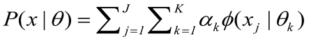 where, xj is j-th observed data, J denotes the number of data points, K represents the number of Gaussian models in mixture model, αk represents probability that the observation belongs to k-th sub model, and θk is the corresponding parameters. A total of 21 data points (7 for each scanning strategy) were expanded to 600 data points corresponding to three different scanning strategies. The augmented data points are constraint within a stress range of 350 MPa to 130 MPa or until the number of cycles reached one million at the corresponding maximum stress. For the fatigue crack growth dataset, the original raw data comprising 446 data points was adopted from the previous study [27]. This dataset includes combined data from all three scanning strategies and covers both the near-threshold and Paris regions of crack growth behavior. As the dataset size is comparable to that of the HCF dataset, data augmentation was not employed.
Before selecting an ML model, it is crucial to transform the experimental data. For the application of the HCF and FCGR prediction models, the training process is expected to be highly time-consuming. To mitigate this, data normalization was applied in this work, scaling the data within the range of zero to unity.
3.2. ML models
3.1.1. Extreme gradient boosting
Extreme gradient boosting is an advanced boosting ensemble technique designed to enhance both predictive accuracy and computational efficiency. It integrates L1 and L2 regularization to reduce overfitting and improve generalization. Using decision trees as base learners, each tree is trained to correct the errors of its predecessors. The algorithm optimizes the training process and model performance by prioritizing speed and accuracy. Additionally, XGB applies gradient descent optimization to minimize the loss function to ensure a closer match between predicted and actual values. Figure 1 depicts the decision-making process, including the root node, intermediate nodes, and leaf nodes. The objective formula combines the loss function with a regularization term as follows [30],
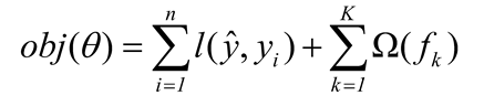 where, l is loss function and Ω(fk) is the regularization term which penalizes the complexity of the tree as,
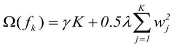
where, γ is a parameter that controls the minimum loss reduction required to make a further partition of number of trees in XGB, K is the number of leaves in the tree, and λ is the regularization term on the weights wj. The processed experimental dataset was divided into training and testing sets, with 80% allocated for training and 20% for testing. Furthermore, the training data was split again, with 80% used for actual training and 20% used as a validation set. The HCF training dataset contained 384 data points, while the FCGR training dataset comprised 286 data points.
Two commonly used metrics for assessing the precision and performance of a machine learning model are the R2 (coefficient of determination) and MSE, as shown in Eqs. (4) and (5).
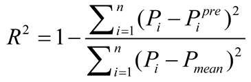
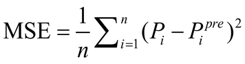 where, Pi represents the ith value in the dataset, Pipre is the ith predicted value, and Pmean denotes the mean of the dataset. A higher R2 indicating a better model fit, where R2 value ranges from 0 to 1. MSE measures the average difference between the dataset and the predicted results, where a smaller MSE indicates more accurate predictions. MSE was calculated on the normalized dataset.
The optimized hyperparameters were determined through sensitivity analysis of two parameters: maximum depth (ranging from 2 to 10) and the number of estimators (100, 200, 400, 500, and 1000). MSE is computed for these values of the parameters and later compared to finding out the optimized hyperparameters. This comparison is illustrated in Figure 2 and the hyperparameters corresponding to the minimum loss values were selected as the optimized hyperparameters. Table 1 presents the optimized hyperparameters for the XGB method for both the tests.
3.1.2. Deep neural network
Deep Neural Network (DNN) is a ML model designed to capture complex input output relationships. As a part of supervised learning, DNNs consist of multiple hidden layers, making them highly powerful for pattern recognition. These networks consists of input layer, hidden layer and output layer [31]. The training process includes both forward and backward passes, where the loss function is optimized using techniques like Gradient Descent and Adaptive Moment Estimation (Adam) [32]. Figure 3 illustrates the full schematic representation of the input, hidden, and output layers.
A typical forward propagation learning process used in the DNN model is given by Eq. (6),
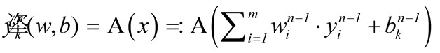 where, the forward propagation output of kth neuron for nth layer is is weight of ith neuron for (n-1)th layer, is the output of ith neuron for (n-1)th layer, is the bias of kth neuron for (n-1)th layer and A(x) is the activation function. For this study, the exponential linear unit (ELU) is used as activation function that can be expressed as [33],
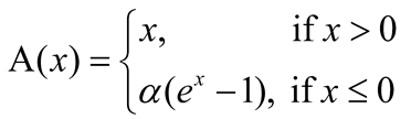
where, x is input to the neuron, α is a constant, and the value is 1. The loss (L) of each layer is calculated in terms of MSE as expressed in Eq. (8) as:
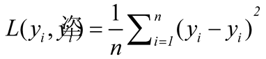
Following forward propagation, the loss function is minimized through backpropagation, as described in Eq. (8), with the help of Adam optimizer. In this method also, the data is divided into two sets: 80% for training and 20% for testing. Furthermore, the training data was split again, with 80% used for actual training and 20% used as a validation set. The hyperparameters were derived from a sensitivity analysis of two factors: the number of hidden layers (ranging from 5 to 40 in increments of 5) and the neurons on each layer (16, 24, 32 and 40). These factors are used to evaluate MSE. The evaluated MSE was compared to finding out the optimized hyperparameters. This comparison is presented in Figure 4 and the hyperparameters corresponding to the minimum loss values were selected as the optimized hyperparameters. Table 2 outlines the optimized hyperparameters for the DNN method in both experiments.
4. Results and Discussion
In this section, the predicted results from both the XGB and DNN models are presented and compared with the experimental results from the previous studies [26,27] A detailed discussion is provided on various aspects of the predictions for all scanning strategies.
4.1. High cycle fatigue
The maximum stress vs. number of cycles curve is a physical–statistical model. It applies empirical formulas (such as Basquin’s equation) to determine parameters that describe the degradation of material strength under fatigue loading. However, ML uses fatigue data to train models and map a nonlinear relationship between the AM process parameters, operating conditions and fatigue life [34,35].
The maximum stress and scanning strategies (S, M, and CH) are considered as input parameters for both models. The output layer contains a single output: fatigue life. The optimized hyperparameters for both models are listed in the previous section. The predicted and actual experimental fatigue life for all the conditions are compared for both models, as shown in Figure 5. The arrows in Figure 5 denote the run-out specimens (more than 1×10⁶ cycles). Additionally, each subplot displays a dashed line corresponding to the 90% survival probability of the specimens. A comparison of the predicted results from models trained on the original experimental dataset indicates that the models perform accurately. For the test dataset, the R2 and MSE are 0.963 and 5.8×10⁻³ for XGB, and 0.961 and 5×10⁻³ for DNN, respectively as shown in Table 3. Both the XGB and DNN models show identical prediction accuracy, as shown in Table 3. Figure 6 (a and b) illustrates the relationship between the loss (i.e., normalized mean squared error) and boosting rounds for XGB model and the epochs for DNN model. The plot shows that the loss rapidly converges to a global minimum, indicating that the XGB and DNN models are well suited to the data and are able to optimize efficiently in a short time. The loss curves are presented for both the training and validation datasets. The predicted data showed good accuracy compared to the actual data, as shown in Figure 7 (almost all data fell within 3 error band).
4.2. Fatigue crack growth
The input parameters for both models include crack length (a), number of cycles (N), stress intensity factor range (ΔK), and scanning strategies (S, M and CH). The output layer produces a single result: crack growth rate (da/dN). The predicted data set and actual experimental data are compared for both models, as shown in Figure 8. This comparison is limited to the Paris region only. The predicted results showed a high degree of accuracy when compared to the actual data, as seen in Figure 8. The prediction results from models trained on the original experimental dataset for FCGR indicate that both models perform accurately. For the test dataset, the R2 and MSE are 0.946 and 1×10⁻⁴ for XGB, and 0.963 and 3×10⁻⁴ for DNN, respectively as shown in Table 4. Among these, the DNN model delivers the higher prediction accuracy, as shown in Table 4. Figure 9 illustrates the relationship between loss (normalized mean squared error) and boosting rounds for the XGB model, and between loss (normalized mean squared error) and epochs for the DNN model. The plot clearly shows that the loss rapidly converges to a global minimum, enabling the model to optimize efficiently in a short period. The predicted data showed good accuracy compared to the actual data, as shown in Figure 10 (almost all data fell within 3 error band).
5. Conclusions
In this study, XGB and DNN machine learning models are used to predict fatigue life and crack growth rate for high-cycle fatigue and fatigue crack growth tests under three different scanning strategies. The key conclusions derived from the observed results and discussions are as follows:
- Both ML models demonstrated similar accuracy and performance on the test data for all three scanning strategies.
- The HCF test data are more sensitive wit hyperparameters as compared to FCGR data set.
- For HCF test data set both models produced nearly identical R2 values, while for FCGR test data set DNN model achieved a higher R2 compared to XGB.
- Both models (XGB and DNN) showed predicted life for the HCF test dataset with more than 90% survivability.
Author Contributions
Conceptualization, V.K.J.; Methodology, V.K.J.; Validation, V.K.J. and R.U.P.; Formal analysis, V.K.J.; Investigation, V.K.J., R.U.P., M.K. and D.B.; Resources, R.U.P. Writing—original draft, V.K.J.; Writing—review & editing, V.K.J., R.U.P., M.K. and D.B.; Visualization, V.K.J.; Supervision, M.K. and R.U.P.; Project administration, M.K. and D.B.; Funding acquisition, M.K. and D.B. All authors have read and agreed to the published version of the manuscript.
Funding
This research received no external funding.
Data Availability Statement
The original contributions presented in this study are included in the article. Further inquiries can be directed to the corresponding author.
Acknowledgments
The authors would like to express their sincere gratitude for the funding and support received from the Ministry of Education (MoE), Government of India.
Conflicts of Interest
The authors declare no conflicts of interest.
References
- Acharya, S.; Gopal, V.; Gupta, S.K.; Nilawar, S.; Manivasagam, G.; Suwas, S.; Chatterjee, K. Anisotropy of Additively Manufactured Co–28Cr–6Mo Influences Mechanical Properties and Biomedical Performance. ACS Appl. Mater. Interfaces 2022, 14, 21906–21915. [Google Scholar] [CrossRef] [PubMed]
- Yoda, K.; Suyalatu; Takaichi, A.; Nomura, N.; Tsutsumi, Y.; Doi, H.; Kurosu, S.; Chiba, A.; Igarashi, Y.; Hanawa, T. Effects of Chromium and Nitrogen Content on the Microstructures and Mechanical Properties of As-Cast Co–Cr–Mo Alloys for Dental Applications. Acta Biomater. 2012, 8, 2856–2862. [Google Scholar] [CrossRef]
- Jenko, M.; Gorenšek, M.; Godec, M.; Hodnik, M.; Batič, B.Š.; Donik, Č.; Grant, J.T.; Dolinar, D. Surface Chemistry and Microstructure of Metallic Biomaterials for Hip and Knee Endoprostheses. Appl. Surf. Sci. 2018, 427, 584–593. [Google Scholar] [CrossRef]
- Hedberg, Y.S.; Qian, B.; Shen, Z.; Virtanen, S.; Odnevall Wallinder, I. In Vitro Biocompatibility of CoCrMo Dental Alloys Fabricated by Selective Laser Melting. Dent. Mater. 2014, 30, 525–534. [Google Scholar] [CrossRef]
- Koizumi, Y.; Chen, Y.; Li, Y.; Yamanaka, K.; Chiba, A.; Tanaka, S.-I.; Hagiwara, Y. Uneven Damage on Head and Liner Contact Surfaces of a Retrieved Co–Cr-Based Metal-on-Metal Hip Joint Bearing: An Important Reason for the High Failure Rate. Mater. Sci. Eng. C 2016, 62, 532–543. [Google Scholar] [CrossRef]
- Park, S.-Y.; Kim, K.-S.; AlMangour, B.; Grzesiak, D.; Lee, K.-A. Effect of Unit Cell Topology on the Tensile Loading Responses of Additive Manufactured CoCrMo Triply Periodic Minimal Surface Sheet Lattices. Mater. Des. 2021, 206, 109778. [Google Scholar] [CrossRef]
- Morettini, G.; Razavi, N.; Zucca, G. Effects of Build Orientation on Fatigue Behavior of Ti-6Al-4V as-Built Specimens Produced by Direct Metal Laser Sintering. Procedia Struct. Integr. 2019, 24, 349–359. [Google Scholar] [CrossRef]
- Xu, Z.W.; Liu, A.; Wang, X.S. The Influence of Building Direction on the Fatigue Crack Propagation Behavior of Ti6Al4V Alloy Produced by Selective Laser Melting. Mater. Sci. Eng. A 2019, 767, 138409. [Google Scholar] [CrossRef]
- Roirand, H.; Hor, A.; Malard, B.; Saintier, N. Effect of Laser-scan Strategy on Microstructure and Fatigue Properties of 316L Additively Manufactured Stainless Steel. Fatigue Fract. Eng. Mater. Struct. 2023, 46, 32–48. [Google Scholar] [CrossRef]
- Cao, Y.; Moumni, Z.; Zhu, J.; Gu, X.; Zhang, Y.; Zhai, X.; Zhang, W. Effect of Scanning Speed on Fatigue Behavior of 316L Stainless Steel Fabricated by Laser Powder Bed Fusion. J. Mater. Process. Technol. 2023, 319, 118043. [Google Scholar] [CrossRef]
- Li, J.; Yang, Z.; Qian, G.; Berto, F. Machine Learning Based Very-High-Cycle Fatigue Life Prediction of Ti-6Al-4V Alloy Fabricated by Selective Laser Melting. Int. J. Fatigue 2022, 158, 106764. [Google Scholar] [CrossRef]
- Ben Chaabene, W.; Flah, M.; Nehdi, M.L. Machine Learning Prediction of Mechanical Properties of Concrete: Critical Review. Constr. Build. Mater. 2020, 260, 119889. [Google Scholar] [CrossRef]
- Xiao, L.; Wang, G.; Long, W.; Liaw, P.K.; Ren, J. Fatigue Life Prediction of the FCC-Based Multi-Principal Element Alloys via Domain Knowledge-Based Machine Learning. Eng. Fract. Mech. 2024, 296, 109860. [Google Scholar] [CrossRef]
- Bao, H.; Wu, S.; Wu, Z.; Kang, G.; Peng, X.; Withers, P.J. A Machine-Learning Fatigue Life Prediction Approach of Additively Manufactured Metals. Eng. Fract. Mech. 2021, 242, 107508. [Google Scholar] [CrossRef]
- Kamble, R.G.; Raykar, N.R.; Jadhav, D.N. Machine Learning Approach to Predict Fatigue Crack Growth. Mater. Today Proc. 2021, 38, 2506–2511. [Google Scholar] [CrossRef]
- Chen, S.; Bai, Y.; Zhou, X.; Yang, A. A Deep Learning Dataset for Metal Multiaxial Fatigue Life Prediction. Sci. Data 2024, 11, 1027. [Google Scholar] [CrossRef]
- Wang, Q.; Yao, G.; Kong, G.; Wei, L.; Yu, X.; Jianchuan, Z.; Ran, C.; Luo, L. A Data-Driven Model for Predicting Fatigue Performance of High-Strength Steel Wires Based on Optimized XGBOOST. Eng. Fail. Anal. 2024, 164, 108710. [Google Scholar] [CrossRef]
- Liu, M.; Wang, X.; Mi, D.; Liu, Z.; Long, X.; Wen, S.; Jiang, C. A New Fatigue Life Prediction Method for Welded Joints Based on Machine Learning Incorporating Defect Information and Physics of Failure. Int. J. Fatigue 2026, 202. [Google Scholar] [CrossRef]
- Guo, K.; Yan, H.; Huang, D.; Yan, X. Active Learning-Based KNN-Monte Carlo Simulation on the Probabilistic Fracture Assessment of Cracked Structures. Int. J. Fatigue 2022, 154. [Google Scholar] [CrossRef]
- Feng, S.; Zhou, H.; Dong, H. Using Deep Neural Network with Small Dataset to Predict Material Defects. Mater. Des. 2019, 162. [Google Scholar] [CrossRef]
- Zhang, X.C.; Gong, J.G.; Xuan, F.Z. A Deep Learning Based Life Prediction Method for Components under Creep, Fatigue and Creep-Fatigue Conditions. Int. J. Fatigue 2021, 148. [Google Scholar] [CrossRef]
- Braun, M.; Kellner, L. Comparison of Machine Learning and Stress Concentration Factors-based Fatigue Failure Prediction in Small-scale Butt-welded Joints. Fatigue Fract. Eng. Mater. Struct. 2022, 45, 3403–3417. [Google Scholar] [CrossRef]
- Zhan, Z.; Li, H. Machine Learning Based Fatigue Life Prediction with Effects of Additive Manufacturing Process Parameters for Printed SS 316L. Int. J. Fatigue 2021, 142, 105941. [Google Scholar] [CrossRef]
- Shi, T.; Sun, J.; Li, J.; Qian, G.; Hong, Y. Machine Learning Based Very-High-Cycle Fatigue Life Prediction of AlSi10Mg Alloy Fabricated by Selective Laser Melting. Int. J. Fatigue 2023, 171, 107585. [Google Scholar] [CrossRef]
- Konda, N.; Verma, R.; Jayaganthan, R. Machine Learning Based Predictions of Fatigue Crack Growth Rate of Additively Manufactured Ti6Al4V. Met. 2022, 12, 1–14. [Google Scholar] [CrossRef]
- Jat, V.K.; Patil, R.U.; Samant, S.S. Influence of Scanning Strategies on the Tensile and Fatigue Properties of Direct Metal Laser Sintering-Printed Co-Cr-Mo Alloy. J. Mater. Eng. Perform. 2025, 34, 7479–7495. [Google Scholar] [CrossRef]
- Jat, V.K.; Patil, R.U.; Yadav, V.K. Fracture Toughness and Fatigue Crack Growth in DMLS Co-Cr-Mo Alloy: Unraveling the Role of Scanning Strategies. Theor. Appl. Fract. Mech. 2024, 134, 104681. [Google Scholar]
- Bera, A.K.; Bilias, Y. The MM, ME, ML, EL, EF and GMM Approaches to Estimation: A Synthesis. J. Econom 2002, 107. [Google Scholar] [CrossRef]
- Shen, L.; Qian, Q. A Virtual Sample Generation Algorithm Supporting Machine Learning with a Small-Sample Dataset: A Case Study for Rubber Materials. Comput. Mater. Sci. 2022, 211, 111475. [Google Scholar] [CrossRef]
- Huang, Q.; Hu, D.; Wang, R.; Sergeichev, I.; Sun, J.; Qian, G. Fatigue Short Crack Growth Prediction of Additively Manufactured Alloy Based on Ensemble Learning. Fatigue Fract. Eng. Mater. Struct. 2025, 48, 1847–1865. [Google Scholar] [CrossRef]
- Zhang, X.C.; Gong, J.G.; Xuan, F.Z. A Physics-Informed Neural Network for Creep-Fatigue Life Prediction of Components at Elevated Temperatures. Eng. Fract. Mech. 2021, 258, 108130. [Google Scholar] [CrossRef]
- Nadda, M.; Shah, S.K.; Roy, S.; Yadav, A. CFD-Based Deep Neural Networks (DNN) Model for Predicting the Hydrodynamics of Fluidized Beds. Digit. Chem. Eng. 2023, 8, 100113. [Google Scholar] [CrossRef]
- Kim, D.; Kim, J.; Kim, J. Elastic Exponential Linear Units for Convolutional Neural Networks. Neurocomputing 2020, 406, 253–266. [Google Scholar] [CrossRef]
- Wang, H.; Li, B.; Gong, J.; Xuan, F.-Z. Machine Learning-Based Fatigue Life Prediction of Metal Materials: Perspectives of Physics-Informed and Data-Driven Hybrid Methods. Eng. Fract. Mech. 2023, 284, 109242. [Google Scholar] [CrossRef]
- Lei, L.; Li, B.; Wang, H.; Huang, G.; Xuan, F. High-Temperature High-Cycle Fatigue Performance and Machine Learning-Based Fatigue Life Prediction of Additively Manufactured Hastelloy X. Int. J. Fatigue 2024, 178, 108012. [Google Scholar] [CrossRef]
Figure 1.
The schematic illustration of the XGB decision tree model architecture.
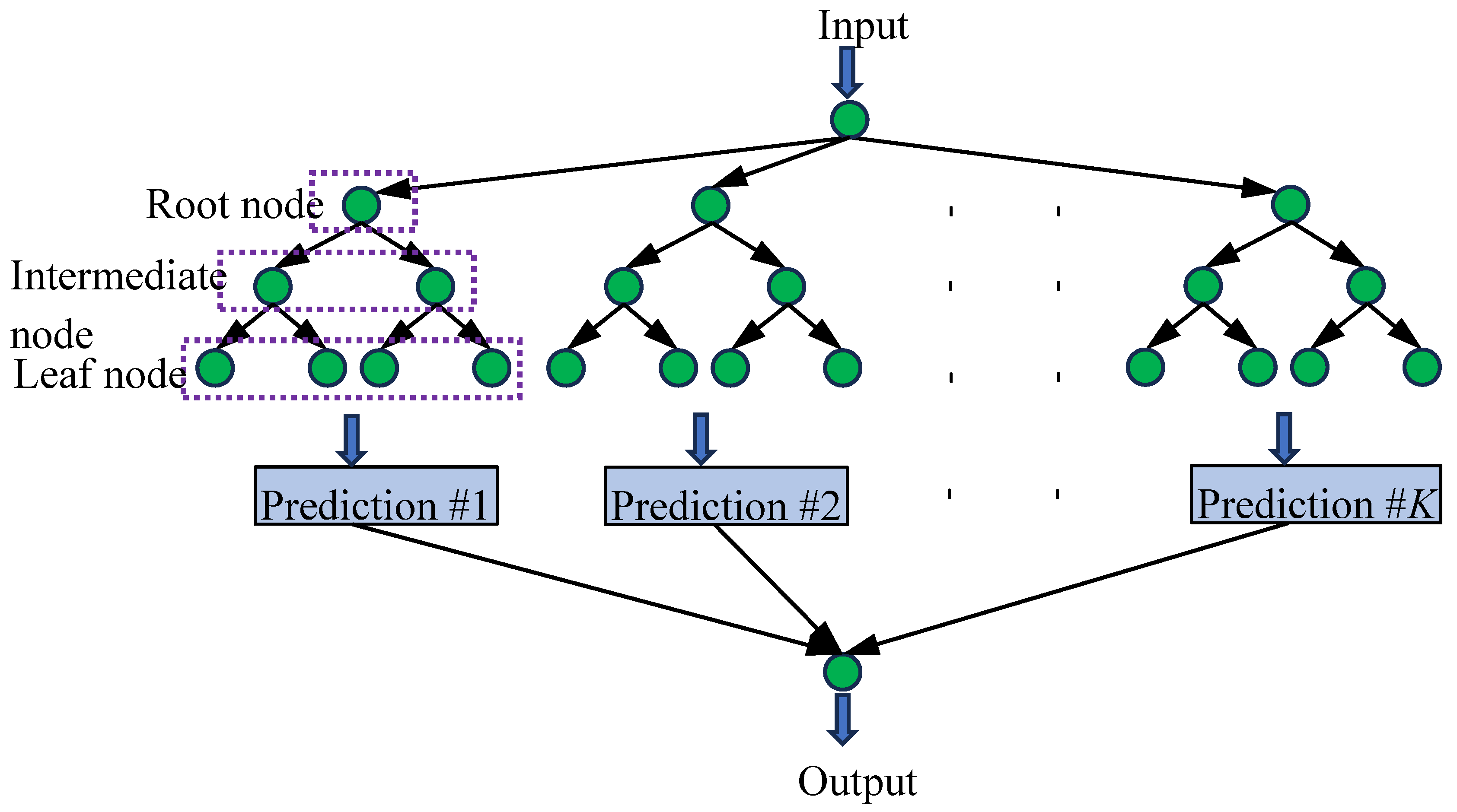
Figure 2.
The hyperparameter sensitivity analysis of the XGB model for both test for (a) number of estimators and (b) maximum depth.
Figure 2.
The hyperparameter sensitivity analysis of the XGB model for both test for (a) number of estimators and (b) maximum depth.
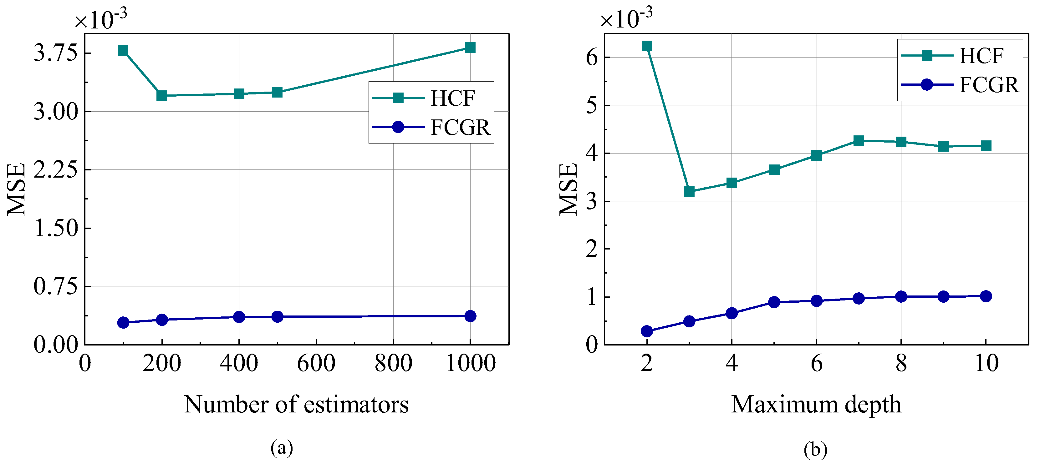
Figure 3.
The schematic illustrations of the DNN model architecture.
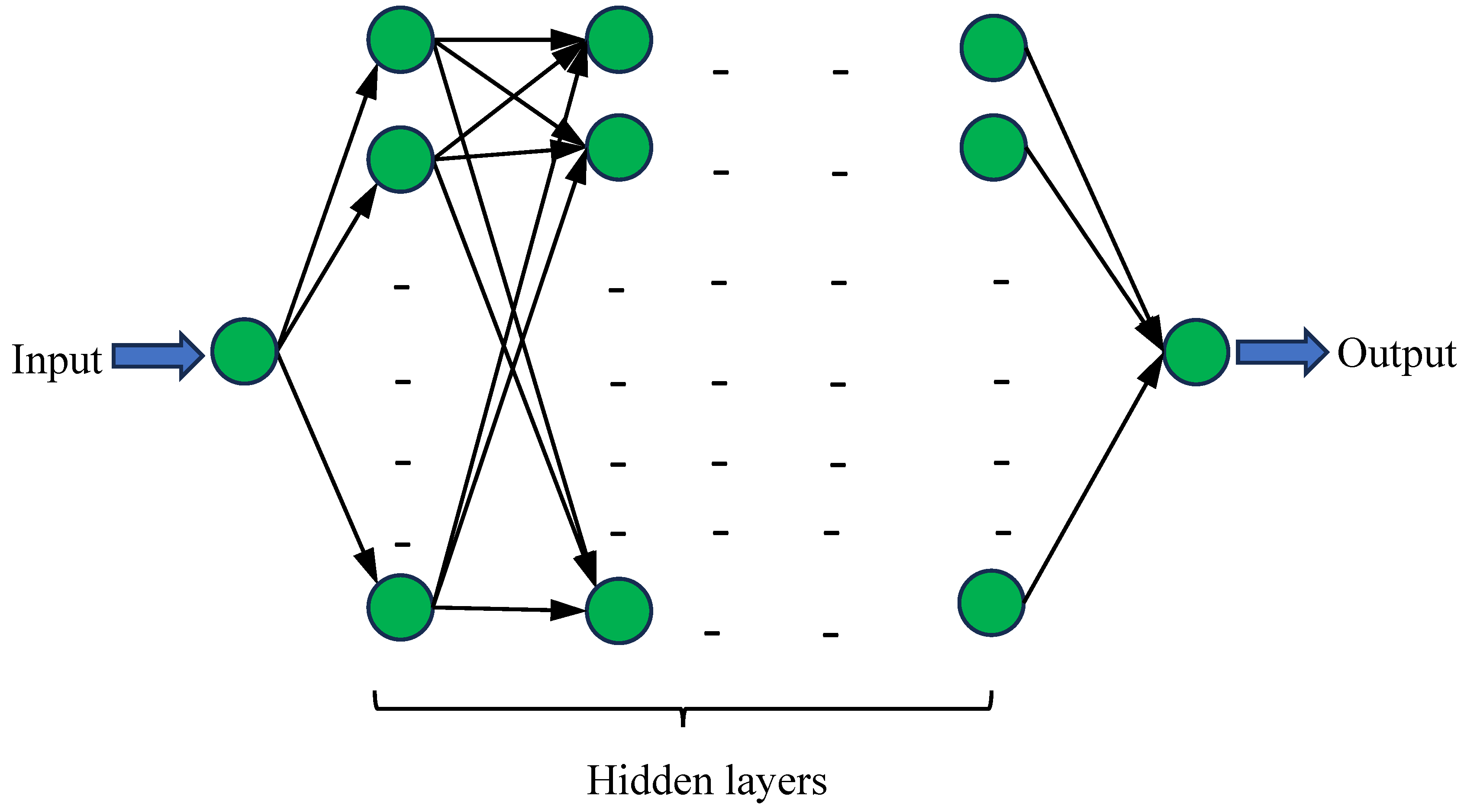
Figure 4.
The hyperparameter sensitivity analysis of the DNN model for both test for (a) number of layers and (b) neurons on each layer.
Figure 4.
The hyperparameter sensitivity analysis of the DNN model for both test for (a) number of layers and (b) neurons on each layer.
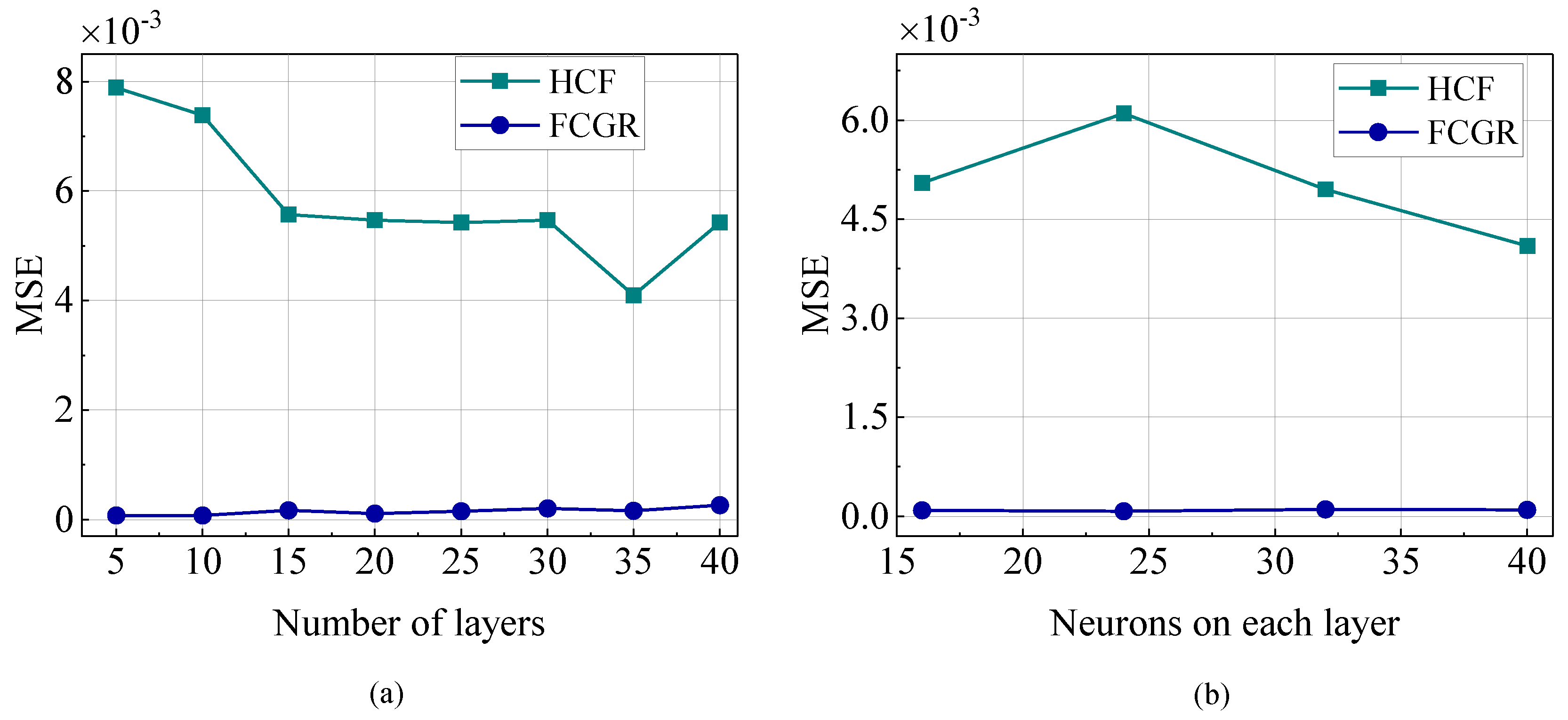
Figure 5.
The maximum stress vs. number of cycle plot for actual experimental data [26] as comparison to predicted data for three different scanning strategy of LPBF printed Co-Cr-Mo alloy for XGB and DNN model.
Figure 5.
The maximum stress vs. number of cycle plot for actual experimental data [26] as comparison to predicted data for three different scanning strategy of LPBF printed Co-Cr-Mo alloy for XGB and DNN model.
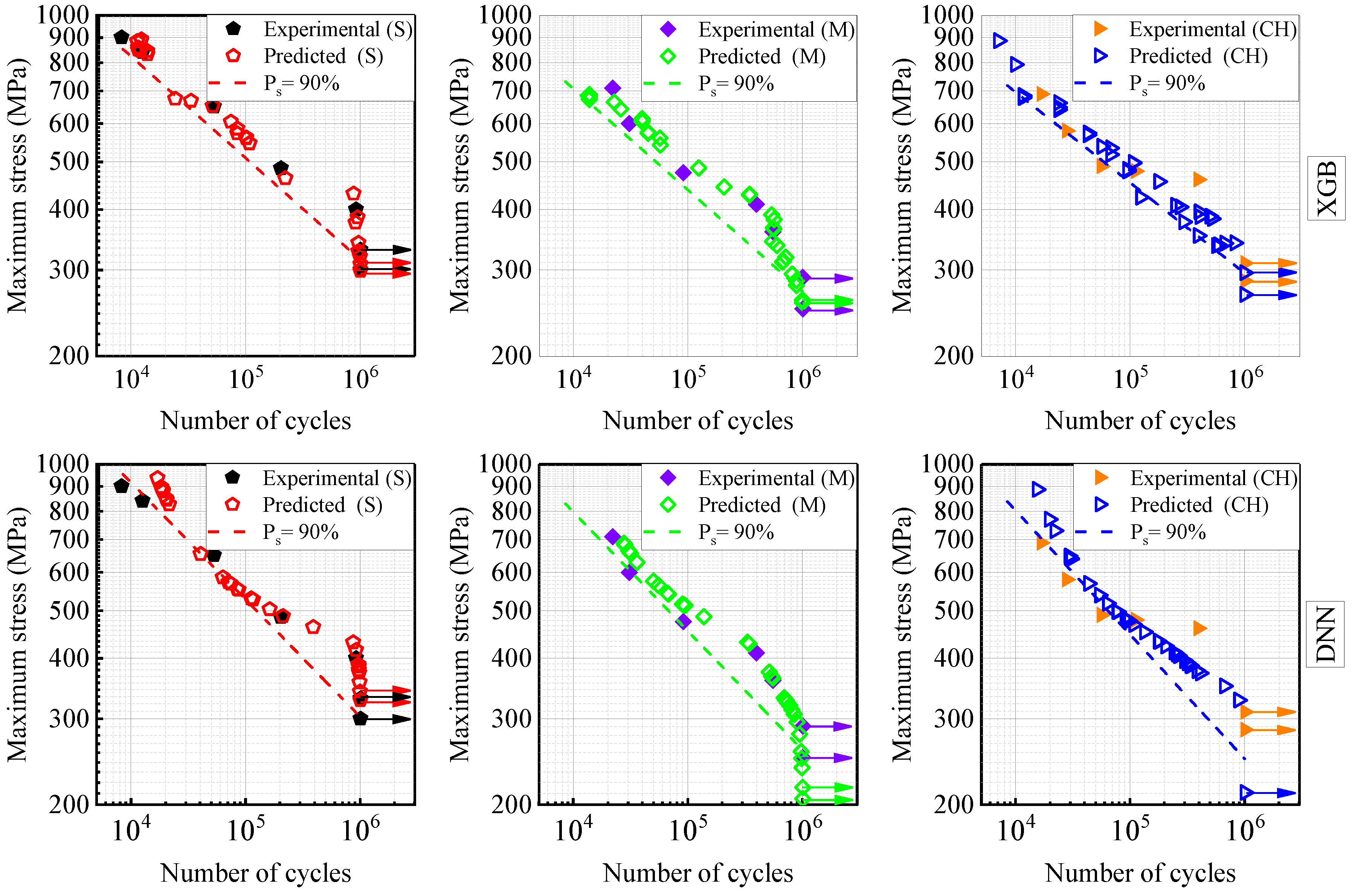
Figure 6.
The loss performance of the (a) XGB and (b) DNN model for HCF data set.
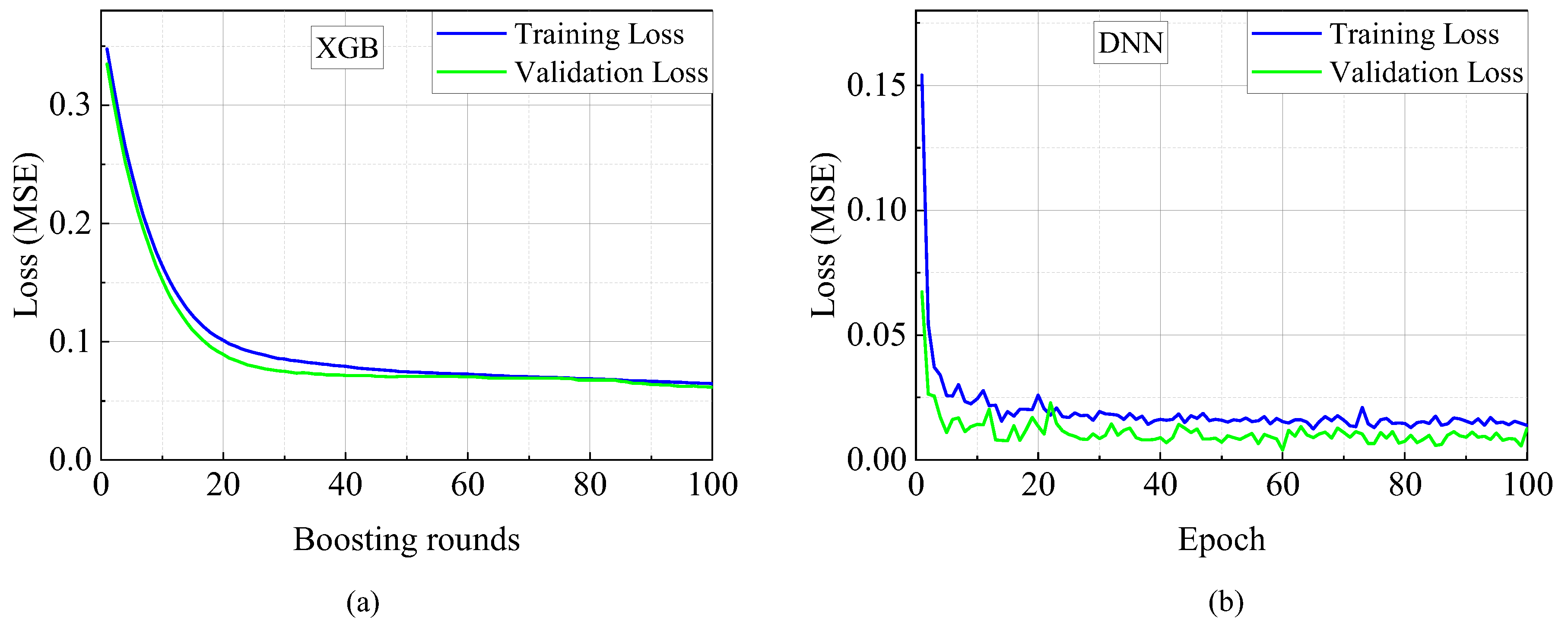
Figure 7.
Predicted fatigue life vs. experimental fatigue life [26] plot for HCF test data set of both XGB and DNN models.
Figure 7.
Predicted fatigue life vs. experimental fatigue life [26] plot for HCF test data set of both XGB and DNN models.
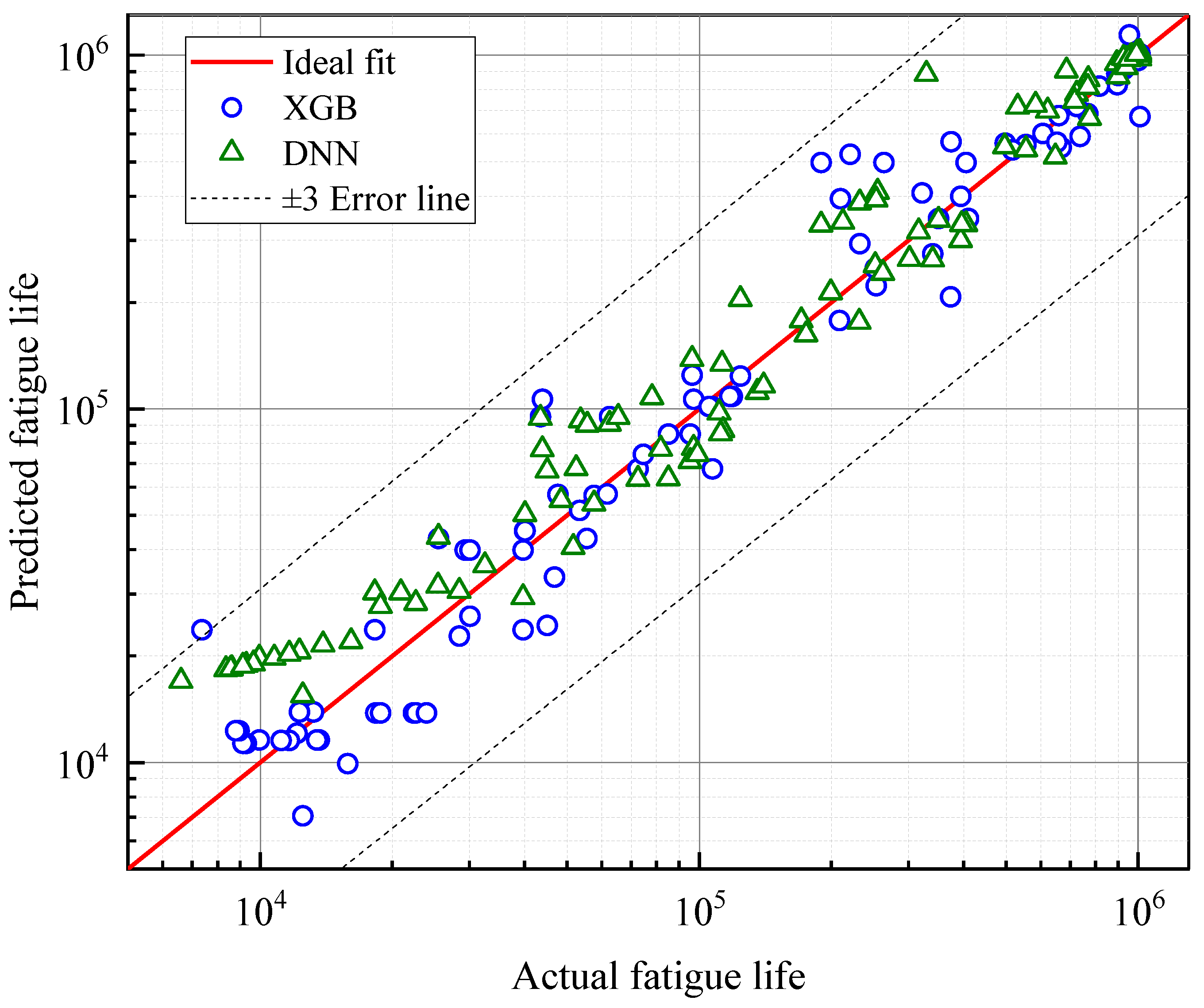
Figure 8.
The plot of stress intensity factor range versus crack growth rate comparing actual experimental data [27] with predicted data for three different scanning strategies of LPBF printed Co-Cr-Mo alloy, based on the XGB and DNN model.
Figure 8.
The plot of stress intensity factor range versus crack growth rate comparing actual experimental data [27] with predicted data for three different scanning strategies of LPBF printed Co-Cr-Mo alloy, based on the XGB and DNN model.
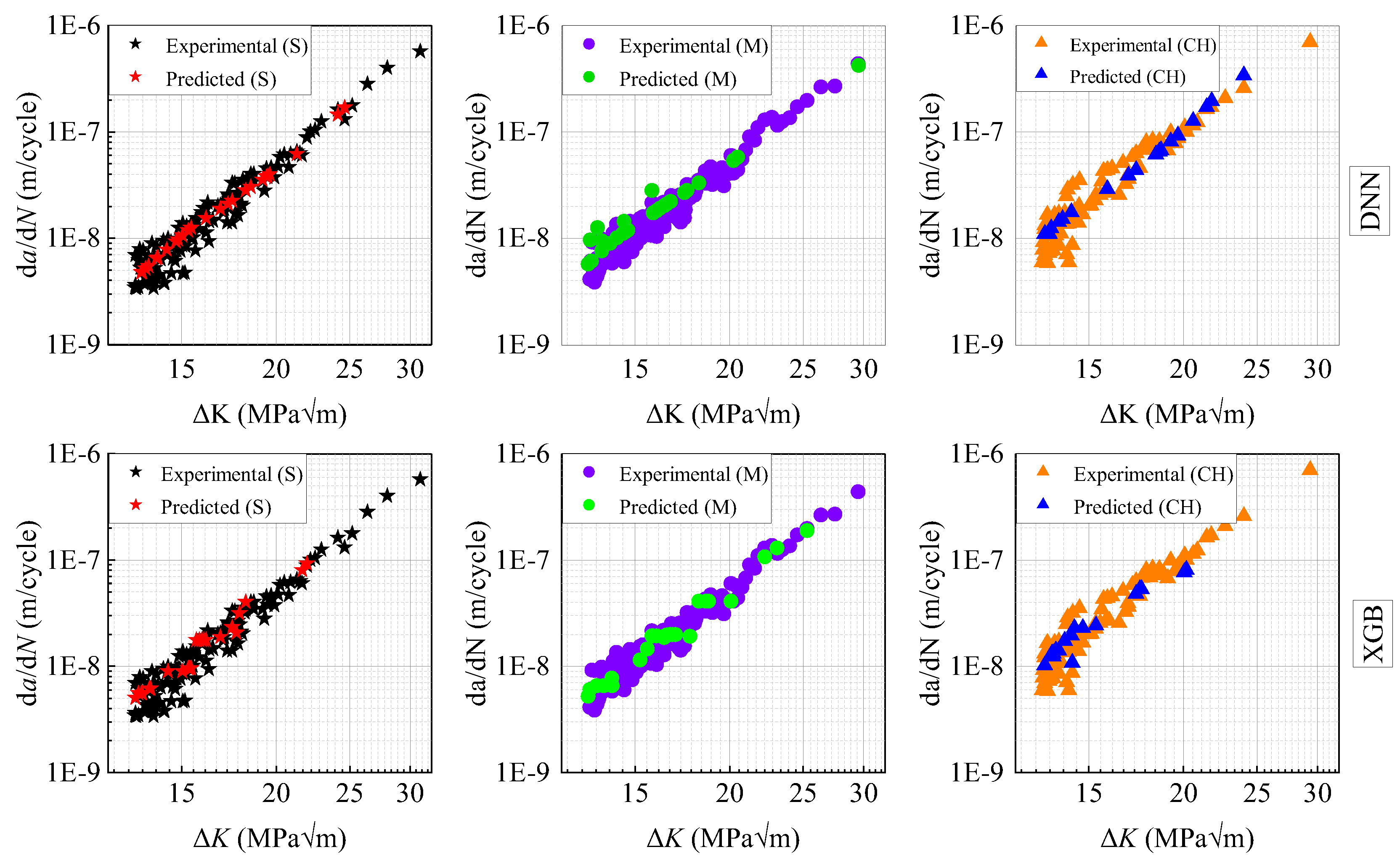
Figure 9.
The loss performance of the (a) XGB and (b) DNN model for FCGR data set.

Figure 10.
Predicted fatigue life vs. actual fatigue life [27] plot for HCF test data set of both XGB and DNN models.
Figure 10.
Predicted fatigue life vs. actual fatigue life [27] plot for HCF test data set of both XGB and DNN models.
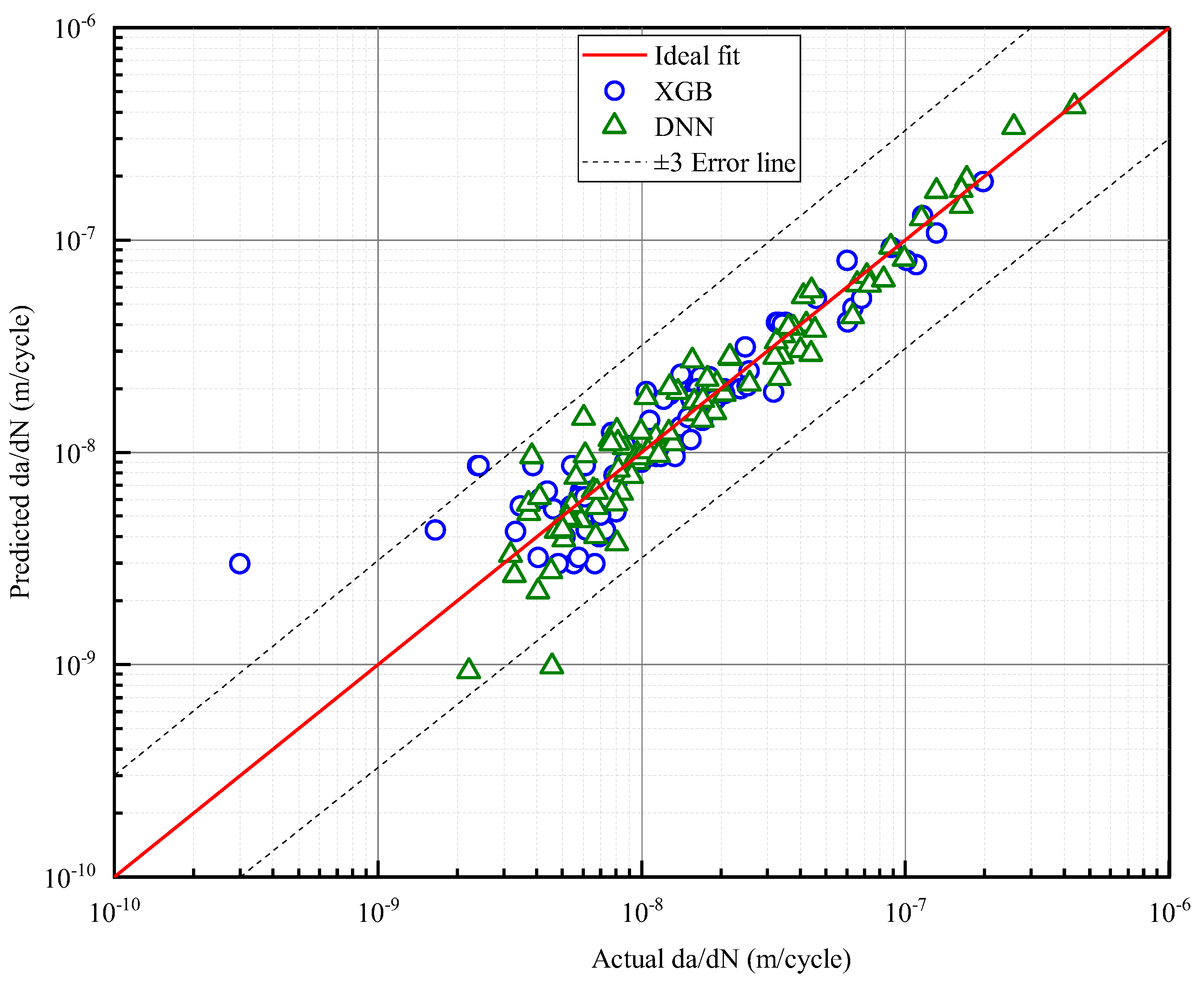

Table 1.
The optimized hyperparameters used in this study for XGB method.
| Hyperparameters | Booster | Learning rate | Regularization term (λ) | Maximum depth | Number of estimators | Min. child weight | Random state | |
|---|---|---|---|---|---|---|---|---|
| Value | HCF | GB tree | 0.1 | 0.2 | 3 | 200 | 2 | 15 |
| FCGR | 2 | 100 | 10 | |||||
Table 2.
The optimized hyperparameters used in this study for DNN method.
| Hyperparameters | Number of Hidden Layers | Learning Rate (Adam) | Neurons on Each Layer | Batch Size | Drop Out | Epochs | Random Seed | |
|---|---|---|---|---|---|---|---|---|
| Value | HCF | 35 | 0.001 | 40 | 24 | 0.02 | 200 | 27 |
| FCGR | 10 | 24 | 15 | |||||
Table 3.
The evaluation metrics for the HCF test predicted test data set for both models.
| Model | R2 | MSE |
|---|---|---|
| XGB | 0.963 | 5.8×10⁻³ |
| DNN | 0.961 | 5×10⁻³ |
Table 4.
The evaluation metrics for the FCGR test predicted test data set for both models.
| Model | R2 | MSE |
|---|---|---|
| XGB | 0.946 | 1×10⁻⁴ |
| DNN | 0.963 | 3×10⁻⁴ |
Disclaimer/Publisher’s Note: The statements, opinions and data contained in all publications are solely those of the individual author(s) and contributor(s) and not of MDPI and/or the editor(s). MDPI and/or the editor(s) disclaim responsibility for any injury to people or property resulting from any ideas, methods, instructions or products referred to in the content. |
© 2025 by the authors. Licensee MDPI, Basel, Switzerland. This article is an open access article distributed under the terms and conditions of the Creative Commons Attribution (CC BY) license (http://creativecommons.org/licenses/by/4.0/).
Copyright: This open access article is published under a Creative Commons CC BY 4.0 license, which permit the free download, distribution, and reuse, provided that the author and preprint are cited in any reuse.


