
Submitted:
17 July 2025
Posted:
18 July 2025
You are already at the latest version
Abstract
The Directed Energy Deposition (DED) process has demonstrated high efficiency in manufacturing steel parts with complex geometries and superior capabilities. Understanding the complex interplays of alloy compositions, cooling rates, grain sizes, thermal histories, and mechanical properties remains a significant challenge during DED processing. Interpretable and data-driven modeling has proven effective in tackling this challenge, as machine learning (ML) algorithms continue to advance in capturing complex property-structure-property relationships. However, accurately predicting the prime mechanical properties, including ultimate tensile strength (UTS), yield strength (YS), and hardness value (HV), remains a challenging task due to complex and non-linear relationships among process parameters, material constituents, grain size, cooling rates, and thermal history. This study introduces an ML model capable of accurately predicting UTS, YS, and HV of a material dataset that comprises 5000 simulation analyses generated using “JMatPro” software, with input parameters including material compositions, grain size, cooling rates and temperature, factors relevant to the DED-processed low alloy steels. Subsequently, an ML model is developed using the generated dataset. The proposed framework incorporates a Physics-based DED-specific feature that leverages “JMatPro” simulations to extract key input parameters such as material composition, grain size, cooling rate, and thermal properties relevant to mechanical behavior. This approach integrates a suite of flexible ML algorithms along with customized evaluation metrics to form a robust foundation to predict mechanical properties. In parallel, explicit data-driven models are constructed using multivariable linear regression (MVLR), polynomial regression (PR), Multi-Layer Perceptron Regressor (MLPR), XGBoost, and Classification models to provide transparent and analytical insight into the mechanical property predictions of DED-processed low alloy steels.
Keywords:
DED
; low alloy steels
; mechanical property prediction
; machine learning
; explainable AI
; process-structure-property relationships
1. Introduction
Metal Additive Manufacturing (AM), especially Directed Energy Deposition (DED), has received considerable interest in manufacturing large-scale components of metallic materials, with complex geometry and tailored microstructures [1]. Unlike traditional subtractive manufacturing, DED is based on a directed heat source, which generally is a laser or an electron beam, to melt and deposit metal feedstock layer by layer, allowing for greater design flexibility, less waste, and faster time to market [2]. However, the complexity of DED with the rapid dynamic thermal cycles, while solidification, formation of the heterogeneous micro-structure, and several microstructural transformations, all make it challenging to find clear processing parameters which govern the resulting mechanical properties [3]. The mechanical response of DED-produced steels depends simultaneously on the interplay of the properties of the alloy, cooling rate, grain size, and thermal gradients, which renders a prediction of the properties a complex task [4]. These aspects are of special interest to critical sectors such as the aerospace and defense industry, where mechanical performance is required to be accurately assessed to control structural quality.
Although microstructural inhomogeneities as well as processing-induced damage, such as porosity, residual stress, or non-equilibrium phases, are inherent to DED-fabricated parts, their detrimental impact on mechanical properties can be frequently mitigated by post-processing methods such as heat treatment or hot isostatic pressing [5,6]. These processes are effective means to improve ductility, strength, and microstructural uniformity. In a number of cases, well-designed, optimally tuned DED parts have shown similarities or even superior mechanical properties when compared to their conventionally processed counterparts, such as cast or wrought steel. However, if the goal is to reduce dependence on post-processes and to better define as-built properties, there is a strong demand for predictive models to accurately predict performance from material parameters and processes. The present study fulfils this need by providing an interpretable, strong ML model that predicts major mechanical properties from DED-specific thermal and compositional characteristics, to improve informed process design and quality control.
Characterizing the mechanical performance of AM-manufactured parts under experimental conditions is currently at a stage where conventional testing methods are high cost, time-consuming, and limited in feasibility. [7]. Experimental studies are typically limited by material-specific setups and explore a specific subset of processing variables, which are difficult to be generalized to other alloys or DED systems. While tools for simulation, such as the finite element method (FEM) or thermodynamic software, are available as an alternative, they often rely on sophisticated calibration, intense computing as well as sequential simulation workflows to predict microstructure evolution and mechanical behavior [8]. For instance, in DED, an effective simulation of material behavior relies not only on the availability and maintenance of the porosity, but also on the ability to simulate the thermal history and the cooling rate in order to predict the final properties [9]. Hence, there is a demand for hybrid methods combining inductive ML methods with physics-based simulations aiming to predict mechanical properties on the basis of dominant process and material parameters with high accuracy and short computation time. The work presented in this study follows a similar hybrid approach, where JMatPro is employed for calculating basic physical properties, whereas ML models are used to quickly and effectively provide generalizations for structure-property relations over broad design spaces.
Evaluation of the mechanical properties of DED-fabricated components is typically limited by being expensive, time-consuming, and resource-intensive for specimen preparation and calibration. Furthermore, experiments usually concern particular alloys and dedicated DED conditions with addition addition-limited range of process parameters. For instance, Akbari et al. [10] introduced a physics-informed ML framework which is trained by experimental data of more than 140 metal AM studies—not limited to processes such as DED—to make accurate predictions of mechanical properties (UTS, YS, hardness) and interpret the impact of features by using SHAP. For example, Sharma et al. [11] built random forest and gradient boosting regression algorithms on a training set of 421 samples and reported high predictive performance (R² > 0.85) for tensile, yield and elongation and that post-processing condition and build orientation were the most important predictors in shaping the mechanical performance in all the three considered properties. Similarly, Mozaffar et al. [12] used a recurrent neural network with Gated Recurrent Units (GRU) for predicting high-dimensional thermal histories in DED, and they reached a test-set MSE of 3.84×10⁻⁵. The model was able to achieve strong modelling accuracy for infrastructure of different geometries and time scales, thus establishing the foundation for data-robust, real-time thermal control measures. Furthermore, Kannapinn et al. [13] proposed a digital twin framework based on neural ordinary differential equations for real-time prediction of residual stress fields and tensile properties during the deposition process by multi-physics DED simulations. Furthermore, predicting mechanical properties such as UTS, YS, and hardness value (HV) through simulations alone is expensive, time-consuming and requires integration of multiple discrete and computationally intensive models.
Given the constraints in experimental datasets, using ML methods to develop models based on simulation data provides a cost-effective and scalable approach to model structure–property relationships for DED-fabricated low alloy steels [14]. Unlike expensive and time-consuming experiments and physical simulations, data derived from thermodynamic tools such as JMatPro, allow a quick assessment of the most important metallurgical characteristics, such as, for example, phase fractions, grain size, or thermal properties over a broad range of compositions and cooling rates [15]. ML models built from such simulation-based datasets are highly flexible and generalize to be able to predict the mechanical properties under different DED conditions and reveal complex input parameter interdependencies. As a result, coupling JMatPro simulations with ML frameworks not only facilitates the accurate prediction of UTS, YS, and HV, but also provides guidance to optimize DED processing parameters to realize the targeted mechanical performance. Despite these benefits, the use of ML in metal AM also has challenges, such as the complexity of features and the small size and limited variance in the simulation-based datasets in comparison with traditional ML applications.
Considering the obstacles and limitations, ML has found applications in Metal AM DED processes. For instance, Rahman et al. [16] employed JMatPro developed mechanical properties data—based on alloy composition, cooling rates, grain sizes and thermal gradients—for more than 2,400 DED produced low alloy steel compositions. They used ML models such as PR and MVLR to predict UTS, YS, and hardness, obtaining R² > 0.79 and showing that simulation augmented datasets can be effectively used to inform mechanical property prediction. Sinha et al. [17] demonstrated a Random Forest Regression model to predict the mechanical properties, such as the Elongation, UST and YS of the alloy steel by using the compositional features and cold rolling deformation. The model had excellent predictive ability of R² ≈ 0.94 for Elongation, 0.99 for UTS, and 0.85 for YS, which presents the power of ensemble learning in materials properties prediction. Furthermore, Era et al. [18] showed that the use of XGBoost outperformed Random Forest and Ridge Regression for the prediction of tensile properties of L-DED parts of SS 316L. Based on input parameters given as laser power, scanning speed, and layer thickness, XGBoost captures the most accurate response with RMSE error of 11.38 MPa (YS), 12.22 MPa (UTS), and 3.22% (elongation). This demonstrated the model’s capacity for mechanical behavior prediction in AM. Qi et al. [19] have predicted YS, UTS, and elongation of low-alloy steels with an average R² of 0.73 using the proposed KD-GCN method compared to classical ML models. It also shows higher consistency (90%) with domain knowledge when analyzing the feature importance than MLP did (70%), which proves its accuracy and interpretability. Chandraker et al. [20] established an ML model which maps alloy composition and DED printing parameters to YS in multi-principal-element alloys (e.g., Co–Cr–Fe–Mn–Ni system). They achieved an R² of 0.84 using ensemble methods like Random Forest and XGBoost, to show the efficiency of ML in predicting mechanical performance from processing inputs. Xie et al. [21] presented a wavelet-CNN model for the accurate prediction of UTS for metal AM based on its thermal history. It surpassed traditional ML, obtaining an R² ~0.70. Certain temperature bands (1213–1365°C and 654–857°C) were observed to have a pronounced effect on UTS. Longer dwell times and quick cooling caused more fine-grained microstructures and better mechanical properties.
Although prior studies have successfully applied ML for advancing the prediction of the mechanical properties of metal AM, they were usually carried out with small experimental datasets, which is very restricting due to the inherent large spread in processing parameters, and with individual materials and build strategies. In contrast, the present study is based on a large and simulation-based dataset, consisting of 4900 instances produced by JMatPro for DED-fabricated low alloy steels. Such a large-scale dataset includes comprehensive input information such as chemical composition, grain size, cooling rate, and thermal property, which can guarantee sufficient training capacity of the ML models for UTS, YS, and HV prediction. Our framework features enhanced generalization by encoding a larger range of material and process variables to enable optimal processes and quality monitoring for a more comprehensive scope of DED processing conditions. This approach allows for a more systematic and physics-based investigation of structure–property relations that are important in advanced manufacturing applications.
With our extensive JMatPro simulated dataset, this work adopts an ML framework for AM to predict mechanical properties—UTS, YS, and HV of DED-manufactured low alloy steels. For assessing the performance of the predicted models, MVLR, PR- Degree 2 and Degree 3, MLPR and XGBoost algorithms were used for predicting the mechanical properties. For the classification, datasets were also trained with classification models to classify ranges of mechanical properties according to DED features like cooling rate, grain size, temperature, and chemical composition. The performance of each model was extensively evaluated in terms of predictive accuracy and interpretability. In addition, this study employed SHAP (SHapley Additive exPlanations) analysis to explain the role of each input feature in making predictions for the ML algorithm. Through physics-based feature creation and interpretable regression and classification models, this framework allows for robust and explainable structure–property prediction in DED-manufactured low-alloy steels.
A key innovation of our framework lies in its ability to generalize across a wide range of alloy compositions and DED processing conditions. By physics-informed featurization— computed using JMatPro simulations, ML models are capable of training a relation for mechanical properties such as UTS, YS, and HV as a function of parameters such as cooling rate, grain size, alloy composition, and thermal behavior that are specific to a DED process. This simulation-driven feature engineering enables the framework to extend its predictive capability to unseen alloy systems and DED parameter spaces, including novel compositions or thermal profiles not explicitly present in the dataset. In contrast to traditional empirical models which were confined to narrow experimental ranges, this study framework provides a flexible and extensible prediction platform to propel the current standard of structure–property modeling in AM, in particular for DED processed low alloy steels.
2. Methodology
This section describes the ML framework, including the process used to acquire and preprocess data from the JMatPro simulations. It also discusses feature engineering based on the parameter of DEDs and the implementation of MVLR, PR (Degree 2 and Degree 3), MLPR, XGBoost and Classification models. To verify and interpret models, the SHAP analysis and standard evaluation metrics are used to verify and interpret the models in predicting the mechanical properties.
2.1. ML Algorithm Framework
The ML algorithm is divided into four main parts: data generation and pre-processing, baseline model learning, feature selection and model simplification, and model interpretation (see Figure 1). First, a full dataset of 4900 JMatPro simulation cases, including physically relevant parameters such as alloy content, grain size, cooling rate, and heat transfer properties for DED processed low alloy steels, was obtained. After the data cleaning and normalization, the training was first performed using two regression models, MVLR, and PR (degree 1 and degree 3). Then, for the improvement of the results, a dataset is used to train MPLR, XGBoost, and classification models to achieve better accuracy and results.
Subsequently, feature importance analysis was investigated based on correlations and model ranking to determine the most influential input features. An involved variant of each model was further retrained using only the top features to facilitate model interpretability and avoid overfitting. Finally, to further understand how certain features influenced predictions of mechanical property (UTS, YS, HV), the SHAP (Shapley Additive exPlanations) analysis was implemented. This individualized substance contribution was, however, useful and interpretable for guiding future alloy design and optimization in DED manufacturing.
2.2. Data Acquisition and Pre-processing
In this study, a comprehensive dataset comprising 4938 sample datasets generated from thermophysical calculations on low alloy DED processed steel carried out in the form of JMatPro simulation software analyses. Each example consists of 13 input descriptors and one of three target mechanical response variables (UTS, YS, and HV). The input features include the full elemental compositions (C, Si, Mn, P, S, Ni, Cr, Mo, Cu, V, Al, N), grain size, thermal exposure temperature (Temp), and cooling rate— all significant factors affecting microstructural evolution. The cooling rate material shows three types of cooling mediums typical of the processing of materials: furnace-cooling corresponding to slow cooling (0.01 °C/s), air-cooling as a model of medium-speed cooling (3.3 °C/s), and ice-brine, fast cooling (375 °C/s). Rigorous preprocessing steps were applied to ensure data integrity, including format alignment, detection of outliers, and normalization of features. The obtained high-fidelity dataset serves as a robust foundation for predictive modeling of mechanical properties in AM.
Data preprocessing is a key step to the dataset training of predictive ML models, as it has a direct impact on the performance, accuracy, and generalizability of these models. This process commonly includes excluding incomplete samples, removing redundant samples, and addressing outliers that can induce biased learning patterns. In this study, missing values were handled using the complete case filtering strategy, retaining only those samples with fully observed features across all input dimensions. The filtering operation is mathematically represented in Eq. (1) [22], where denotes the data point and , its corresponding feature value:
where:
- = original dataset with n samples and m features
- = ith data sample
- = value of the feature in the sample
- = filtered dataset containing only complete records
This equation means that only the samples for which the values of the features are valid and not missing (i.e., not NaN) are retained for subsequent modelling. Here, NaN is the abbreviation for “Not a Number”, used to represent an undefined or missing number in a data set which typically results from incomplete simulations, corrupted input data, or format irregularities.
As a result of this filtering, the dataset used for the regression-based algorithm consists of MVLR, PR, MLPR, and XGBoost models used for 4900 samples after filtering, cleaning, deduplicating, and handling missing values. This ensured that only complete and consistent data contributed to the ML algorithm’s dataset training and evaluation. In contrast, the classification model dataset of 4900 samples, as the pre-processing step focused on label binarization and class balancing, not involving sample removal. No automated outlier detection (e.g., Mahalanobis distance or Z-score) was conducted, however, inspection of input feature distributions assured that all samples remained consistent. Duplicate entries were inherently excluded due to unique simulation configurations. The retained variability in chemical composition, grain size, thermal input, and cooling rate presented a large and diverse feature space suitable for both regression and classification model tasks. Table 1 illustrates a statistical overview of several labels within the dataset, incorporating their mean, median, and standard deviation. The descriptive statistics provided in this paper will highlight the spread and features of the data, thus providing an important insight into the general nature of the data.
2.3. Dataset Featurizations
To ensure robust and generalizable predictions for mechanical properties, a dedicated and physics-based feature selection approach was employed during ML models training. The featurization approach employed in this work combines material-related as well as process-informed features acquired from extensive simulations generating the low-alloy steel-based alloy using JMatPro. Specifically, elemental compositions (i.e., C, Mn, Si, Cr, Ni, Mo), grain size, cooling rate, and thermal history, all of which are known to decisively impact mechanical behavior in DED-produced low alloy steels. These characteristics, collated in Figure 2, are from the foundation of the dataset and represent domain knowledge for the understanding of complex structure–property relationships for DED fabrication.
Besides process parameters and material compositions used to generate continuous variables, the featurization framework includes some categorical features to capture essential qualitative distinctions within the dataset. As illustrated in Figure 2, the categorical input (e.g., alloy code: MBB, MBC) represents key identifiers that differentiate compositional families or experimental groupings relevant to the DED process. These categorical variables are converted to machine-readable form via one-hot encoding where a binary vector of size 1×n is used to express each category, with “1” assigned to the index and zeros assigned to the rest of the indices for any data point that belongs to the category. This encoding framework is implemented so that ML models can understand and learn discrete differences between alloy classes without adding prediction tasks. While this study analysis is focused on alloy code as a categorical input, it demonstrates that the featurization method can be straightforwardly applied to other types of input features such as process parameters and material composition. To confirm the consistency and completeness of the training datasets with the absence of any of the necessary categorical or continuous aspects is removed. This pre-processing ensures that data used as input can provide a full feature set for both training and evaluation, thereby promoting more consistent and reliable model training and evaluation.
2.4. Models Evaluations and Verification Strategy
To comprehensively evaluate the prediction accuracy of the developed models, both regression-based and classification-based evaluation strategies were used. These combined methods enabled robust validation of both continuous and discretized outputs for mechanical property prediction of DED-manufactured low alloy steels.
For regression tasks involving MVLR, PR, MLPR, and XGBoost algorithms performance was quantified using four standard error-based metrics which are Mean Absolute Error (MAE), Root Mean Squared Error (RMSE), and the Coefficient of Determination (R2). The equations are as follows in Equations (2)–(4) [23,24,25]:
where and represent the predicted and observed values of the sample, is the mean of the observed values, and N denotes the number of data points. These measurements define an adaptive regression rule based on absolute and squared deviations from predictions to labels, offering a sound assessment of the accuracy and generalization of the regression model. The better model performance depends on the lower value of MAE, RMSE, and the higher the value of R2.
To complement regression analysis, a classification framework was used to interpret model performance when the continuous mechanical property outputs were transformed into categorical bins (i.e., low, medium, and high hardness). The confusion matrix and its derived metrics- accuracy, precision, recall, and F1-score were used to report the performance. This was supplemented by multiclass Receiver Operating Characteristic (ROC) curves and Area Under the Curve (AUC) analysis, giving an overview of the discriminatory power of the model across the different classes.
To enhance ML model reliability and minimize bias caused by data heterogeneity, rigorous cross-validation techniques were integrated into the validation strategy. In particular, cross-validation used in this study, the dataset was split into subsets, and the subset of the data was used as a test set while the rest was used as training data one at a time. K-Fold and Stratified K-Fold cross-validation (CV) were employed to maintain the class balance between the folds, and leave-one-out cross-validation (LOOCV) is also used to ensure the evaluation results are statistically robust and generalizable. The best resulting model, according to cross-validation loss, was chosen and saved for each mechanical property task. This comprehensive evaluation system, comprising continuous and discrete measures, multilayered cross-validation, and optimized learning parameters, guarantees accurate prediction and interpretability of mechanical behaviors in DED-manufactured low alloy steels.
This dual-framework approach integrates regression-based precision with classification-based interpretability, provides full model verification, and demonstrates the potential of the developed ML algorithm framework in estimating the mechanical properties based on the process-dependent features in DED-processed low alloy steels.
2.5. ML Algorithms
This section provides the ML algorithms used to predict mechanical properties- UTS, YS, and hardness of the futurized dataset based on JMatPro simulations of DED fabricated low alloyed steel. The algorithms used are Multivariable Linear Regression (MVLR), Polynomial Regression (degree 2 and 3), Multi-Layer Perceptron Regressor (MLPR), Extreme Gradient Boosting (XGBoost), and classification models that are then employed to enhance predictive accuracy and comparative analysis.
2.5.1. Multi-Variable Linear Regression (MVLR)
MVLR is an important statistical technique for studying the linkage of a dependent single variable to several independent variables. MVLR serves as a simple and easy-to-use reference model for the prediction of mechanical properties of DED-processed low alloy steels [26]. The model assumes a linear relationship between the input features -chemistry composition, cooling rate, and process parameters and target outputs- UTS, YS, and HV. The model estimates coefficients for each input variable that best fit the data by minimizing the difference between the observed and the predicted values -Residual sum of squares (R2). MVLR is formulated to solve the following equation in symbolic notations, in mathematical expressions shown in Eq.1 [27]:
where is the predicted mechanical property, is the input characteristics and is the learned coefficient. One of the main advantages of MVLR is the high interpretability, which permits explicit quantification of the contribution of each processing or compositional variable to the mechanical response. This is particularly beneficial for understanding metallurgical trends in DED-produced steels. However, MVLR rests on some assumptions such as linearity, homoscedasticity, and no multicollinearity. To make good predictions, pre-processing includes feature engineering and correlation analysis. Despite its simplicity, MVLR is a method that provides interesting hints and serves as a robust benchmark to be compared with more complex models applied within this work.
2.5.2. Polynomial Regression (PR)
PR extends the concept of linear regression by including polynomial terms in the input features so that the model can detect non-linear correlations between the features and the output [28]. PR is employed in this work (Eq. 2) for the complex non-linear interrelations of DED process parameters, alloy compositions, UTS, YS, and hardness. The following Eq. (06) describes the PR model [29]:
Here, represents the predicted mechanical property, and x is the input variable(s), are the coefficients obtained by training. This formulation allows PR to be capable of conforming not only to linear lines but also to curves, thereby enhancing its capacity to model real material properties where the linear approximation is not sufficient. However, such an assumption may oversimplify the inherent physics-driven interactions in DED-processed steels. Hence, polynomial models—particularly PR degree 2 and degree 3—are incorporated to better fit the observed curvature in mechanical response behavior due to interactions between grain size, cooling rate, and alloy composition.PR Degree 2 and Degree 3 Equations (7) and (8) are as follows [29]:
One major strength of PR is its flexibility, as it can effectively model non-linear relationships in the data with low computational cost. In the context of DED processed steels, this is a great advantage to study the influence of subtle variations in thermal history and composition on mechanics [30]. However, increasing the degree of the polynomial increases the complexity of the model, which could lead to overfitting unless regularization techniques are applied [30]. To account for this in the model tuning, procedures of polynomial degree selection and validation were applied to ensure generalization and prevent high variability.
2.5.3. Multi-Layer Perceptron Regressor (MLPR)
MLPR model, which is a feedforward artificial neural network model that maps sets input data onto a set of appropriate outputs. It includes the input layer, one or more hidden layers with non-linear activation functions such as ReLU or tanh, and an output layer that emits continuous results for regression. Every neuron computes a weighted sum of its inputs and applies a non-linear transformation, which makes the network capable of learning complex patterns. The model is trained by appropriating and optimizing a loss function, often the MSE— with gradient-based optimizers such as Adam, or LBFGS. The model architecture of MLPR used in this study has only one hidden layer and is mathematically expressed in Eq. (9) [31],
where is the predicted mechanical property and x the input feature vector, and are the weights and biases of the hidden layer, σ (⋅) denotes the activation function, and , are the weights and biases of the output layer. The model was fitted using the Adam optimizer with ReLU activation and MSE loss, in addition to the following hyperparameters: hidden layer size = 100, learning rate = ‘adaptive’, alpha = 0.0001, and max iterations = 1000.
In the context of this study, MLPR was used to describe intricate non-linear relationships between DED-processing parameters, such as cooling rate, grain size, alloy composition, and properties -UTS, YS, and HV. In contrast to the conventional linear models, the MLPR provides more flexibility by learning hierarchical feature representations, which is most promising for modeling high-dimensional structure–property relationships where the linear assumption fails to capture interaction effects.
2.5.4. Extreme Gradient Boosting (XGBoost)
XGBoost is an ensemble ML algorithm that builds a sequence of weak learners, usually decision trees, and combines them to construct a predictive model. Compared to traditional decision trees, XGBoost adopts gradient boosting with more advanced regularization (both L1 and L2), tree pruning, and parallelized training to minimize a differentiable loss function as an additive model updates and is characterized by its high accuracy, efficiency, and scalability to complex, non-linear datasets. Given an input x, the prediction of XGBoost can be formulated as in Equations (10)–(12) [32]:
Here, is the prediction for the sample, and K is the number of regression trees. The function (⋅) denotes the regression tree that contributes to the overall model prediction. The space refers to the set of all possible regression tree functions, where each tree maps an input from the feature space to a real-valued output in R.
Here, is the loss function applied to quantify the gap between the predicted and actual values, which can be, for instance, squared error: . The regularizer is the regularization instead of the kth regression tree and is used to maintain the complexity of the model. T is the number of leaves in each decision tree, and wj is the weight of the leaf node. The regularization terms γ and λ penalize the number of leaves and the absolute values of leaf weights, respectively, which encourage simpler models with better generalization performance over unseen data.
In this work, XGBoost is implemented for the establishment of non-linear regression models between process parameters of DED (composition, grain size, cooling rate) and the related mechanical properties (UTS, YS and hardness). Its immunity to overfitting, the ability to process multicollinearity, and the feature importance analysis, indicate its great suitability to high-dimensional materials data from JMatPro simulations.
2.5.5. Classification Model
The predictive performance and generalization capability of the classification models for the training score and test score is used to evaluate the models based on classification accuracy. The training score measures how well the model is performing on the training dataset and the test score on the test dataset. These measures are calculated as the percentage of samples that are correctly classified from the set. Balanced performance in the two scores suggests better generalization, while a significant difference between the values may indicate underfitting or overfitting. The equations are as below in Equations (13) and (14) [33],:
Here, the predicted class labels for the training sample and test sample, respectively; and are their corresponding true class labels. and represent the total number of training and test samples.
Additionally, classification accuracy was assessed with confusion matrix-based metrics including accuracy, precision, recall, and F1-score, for each class, averaged with both the macro and the weighted approach in Equations (15) to (19) [34]. To evaluate the model’s ability to distinguish among multiple classes, multi-class ROC curves (via the one-vs-rest method) and the corresponding area under the curve (AUC) with the macro averaging and weighted averaging in Equations (20) to (22) [35]. These all-inclusive performance criteria verify the efficiency and dependability of the proposed ML models for predicting the mechanical properties of DED-manufactured low alloy steels.
Precision (per class):
Recall (per class):
F1-Score (per class):
Macro-Averaged F1:
where TP, TN, FP, and FN are the number of true positives, true negatives, false positives, and false negatives. Precision measures the ratio of correctly predicted positive observations to the total predicted positives (positive predictive value), while recall measures the ratio of correctly predicted positive observations to all observations in the actual class. The F1-score is the harmonic mean of precision and recall, which provides a trade-off between them. Where, in a multiclass framework F1c is the F1-score for class c, and C is the number of classes. Macro-averaged F1 score is taken as the unweighted average of F1 scores across all classes to make sure all classes contribute equally.
Multiclass ROC-AUC (OvR) Equation:
Then, the overall macro-average AUC,
Here is the True Positive Rate as a function of the False Positive Rate for class ccc in a one-vs-rest (OvR) multiclass classification. Namely, the AUC for class c, noted , is obtained by integrating over [0,1] with respect to the false positive rate. The macro-averaged ROC-AUC score, , is calculated as the average of individual class-wise over all C classes
To further ensure robustness, cross-validation methods are used, such as K-Fold, Stratified K-Fold, and Leave-One-Out Cross-Validation (LOOCV). In K-Fold CV, the dataset is divided into K subsets that are used for validation (K-Fold) and for training (rest of the K−1 Folds). Stratified K-Fold builds upon it by keeping the class distribution through them, which is a very useful option for imbalanced datasets. Leave-one-out-cross-validation (LOOCV), a special case of K-Fold with K = N, trains on all but a single data point and tests that single point for any parameter; LOOCV uses all available data at the expense of computational cost. The equations are as follows in Equations (23)–(25) [36],
K-Fold Cross Validation:
Stratified K-Fold,
Leave-One-Out Cross Validation (LOOCV),
Here, is a performance measure (such as accuracy, F1-score, or RMSE) in the fold or iteration. Here, K is the sum of all folds in K-Fold and Stratified K-Fold cross-validation, and N is the count of all samples in the dataset for the Leave-One-Out Cross Validation (LOOCV).
3. Results and Discussion
This section provides a detailed analysis of the prediction performance of the ML models proposed for UTS, YS, HV mechanical properties by JMatPro simulated dataset on DED-processed low alloy steels. The focus is given on the regression and classification performance of models like MVLR, PR, MLPR, and especially XGBoost and the results are validated by error metrics, confusion matrices, SHAP analysis, and cross-validation methods.
3.1. ML Algorithms Results
3.1.1. Quantitative Model Evaluation
The predictive performance of five regression algorithms—Multivariable Linear Regression (MVLR), Polynomial Regression (PR) with degrees 2 and 3, Multi-Layer Perceptron Regressor (MLPR), and XGBoost were systematically evaluated to predict the mechanical behavior for DED-fabrication of Low Alloy Steels. The detailed error matrix- MAE and RMSE, and determination coefficients- R² values corresponding to UTS, YS, HV predictions are listed in Table 2.
MVLR presented as the baseline model that provided R² of 0.82, 0.79, and 0.83 for UTS, YS, and HV, respectively. These results imply that though linear correlations between compositional and thermal features, MVLR does not have the capacity to approximately capture higher-order dependencies, particularly within domains where compositional phase transformation interacts non-linearly with thermal steep gradients. The PR with degree 2 achieved only very slight improvement, suggesting that the square term in the second-order polynomial model is not enough to capture the complex feature interactions that are inherent to DED processes.
In contrast, PR of degree 3 significantly improved prediction accuracy with R² of 0.91 for UTS and HV and 0.88 for YS. These significant improvements are a consequence of the improved flexibility of the model to capture multivariate non-linear relationships which are associated with the effects of cooling rate and the alloying element on the transformation-induced strengthening and hardenability [36,37]. The MAEs for PR with degree 3 were reduced to 50.79MPa UTS, 56.95MPa YS and 2.26 for HV with all the data involved in the model indicating the model has strong adaptability to a variety of property scales for the low alloy steels.
The MLPR model also further outperformed polynomial approaches, reporting R² values of 0.94 for UTS, 0.93 for YS, and 0.93 for HV, with the corresponding MAE values closing to 38.03 MPa, 36.94 MPa and 1.68, respectively. This result confirms the capability of the neural network in learning non-linear, higher-dimensional maps between compositional and thermal features and mechanical responses, in the absence of explicit feature engineering or transformation terms.
The highest accuracy was obtained with the XGBoost model and R² values of 0.98 in all properties for estimation purposes. The corresponding MAEs values—15.40 MPa for UTS, 15.43 MPa for YS, and 0.556 for HV—are the lowest recorded errors among all tested models. This result shows that XGBoost is not only capable of capturing non-linear feature hierarchy but also maintains strong generalization performance without overfitting. From a materials modeling standpoint, the low prediction errors presented in this study strongly indicate highly acceptable and relevant, especially given the inherent complexity of DED-fabricated steels, where the mechanical response is controlled by a combination of microstructural heterogeneity and thermal history effects [38].
From a recent scientific perspective, the trend in performance observed in this study and provides support to the hypothesis that model architecture based on an ensemble with a decision tree backbone, such as XGBoost, are well suited for the prediction of structural property relationships in the context of AM. These results are in line with previous work in metal AM where ensemble models were shown to outperform linear and neural network-based regressors on problems involving complex PSP linkages. Overall, the prediction accuracy obtained in this work not only demonstrates the ability of the proposed ML model but also introduces a reproducible baseline for the future big data-based modelling of DED-processed steels applications. From an industrial point of view, such model prediction frameworks that can reproduce property value accurately can potentially speed up material qualification and validation, reduce the number of iterations on the experimentation loop, and help to develop closed-loop control systems in the context of future AM processes.
3.1.2. Visual Evaluation of Model Predictions
To further evaluate model performance, actual vs predicted plots were also drawn for each of the ML algorithms for the three mechanical properties- UTS, YS, and HV in Figure 3. These plots serve as a graphical diagnostic of the model’s predictive accuracy and the ability of the model to be generalized over the range of observed values.
The results of the MVLR model are shown in Figure 3a to Figure 3c. Although there is a linear trend between the predicted and actual outputs in general, a large spread of data points is also observed, especially for the higher values of the UTS and YS. The UTS plot (Figure 3a) indicates a higher degree of scatter at strengths in excess of 1400 MPa whereas it is observed for the YS predictions (Figure 3b) between 600–1000 MPa. Similarly, the HV predictions (Figure 3c) differ at both ends of the range, especially at less than 10 HV and more than 45 HV, indicating the model’s limited capacity to capture complex thermomechanical relationships.
Figure 3d to Figure 3f display the performance of the PR algorithm. These plots indicate the MVLR results, with comparable trends in deviation and similar clustering around the mean. While PR does introduce some non-linearity in the model, it does not summarize higher-order interactions of the higher-order polynomials, as shown by the remaining large residuals from the extreme values. Although PR substantially improves prediction quality, plots for this model are shown here. This improvement is reflected in the evaluation metrics, with R² increasing from 0.82 to above 0.90, demonstrating the advantages of adding higher-degree polynomial terms to represent non-linear feature interactions.
Figure 3g–Figure 3i show the predictions obtained from the MLPR model. Here, a substantial decrease in the prediction error is observed for all properties. In the UTS plot (Figure 3g), predictions closely trace the 1:1 diagonal line with little disturbance by the residuals, with a similar touching for the YS plot (Figure 3h), with some overprediction in the mid-strength range. The prediction of hardness (Figure 3i) seems to be especially well modeled with dense data clustering around the ideal fit line, a clear indication that the model can effectively relate the compositional and thermal factors to the mechanical performance. These findings demonstrate the potential of neural networks to capture complex and non-linear structure-property relationships, particularly with complex feature-rich datasets in big datasets.
Finally, Figure 3j–Figure 3i show the predictions of the XGBoost, which presents the highest prediction accuracy among all algorithms. For the UTS and YS in the Figure 4j, 4k diagrams, both entire and arranged, are uniformly presented with the closest relationship of predicted and actual values across the entire range, including both lower and upper extremes. The prediction of hardness (Figure 3i) stands out for its precision, with predicted values very close to overlapping with the identity line. This model performance demonstrates the prediction accuracy and the robustness of the XGBoost model on representing multi-level, non-linear feature interactions as well as controlling overfitting. The ensemble nature of XGBoost also allows it to generalize across a diverse set of complexes and high-dimensional datasets, which are especially relevant for AM applications, as microstructural changes with process history significantly influence final properties.
Together, these plots demonstrate that although linear and low-order polynomial models serve as a baseline, more sophisticated ML models, and especially MLPR and XGBoost, can greatly improve the prediction performance and generalization ability. The visual overlap between predictions and ground truth using XGBoost further supports its efficacy in capturing the complex structure–process–property relationships inherent to DED alloy fabrication.
3.1.3. XGBoost Model Residual and Distribution Error Plots
Residual Plots
The distribution errors in XGBoost model predictions were assessed both in the residual plots, model bias, variance, and evaluated across the predicted range for UTS, YS, and Hardness. Figure 4 shows the residuals- actual Vs predicted values as a function of the true values of the target for each of the mechanical properties.
In the UTS residual plot Figure 4a, the residuals are generally centered around zero, which is the majority falling within ±100 MPa. Some outliers are observed below 600 MPa and above 1400 MPa, but without a clear pattern or curvature. This indicates that the XGBoost model is well calibrated and unbiased for the UTS spectrum, and a slightly larger variation in the middle to high strength range is evident.
The YS residual plot Figure 4b shows that visualized residuals mostly clustered and most of the residuals are concentrated around the zero line, and the model has disadvantages of less than ±100 MPa of the predictions. Some bigger residuals are present within the 500-1000MPa range, but they are randomly distributed without a systematic trend. This implies the model is not heterogeneous with equality, which is increasing variance with increasing strength, and that the prediction error is uniform across all the classes.
The residual plot (Figure 4c) of the Hardness shows the tightest residual distribution between the features, and most of the errors lie within ±5 HV and with the center close to zero. There is no observable trend or systematic bias, and the errors are evenly spread across 0 to 50 HV values. This is consistent with the previously noted high R² and low MAE/ RMSE for hardness, confirming that XGBoost is highly accurate and consistent in capturing thermal-compositional effects on microstructural hardness.
Overall, the residuals of three properties exhibit random scatter and no observable systematic deviation, satisfying the assumption of model accuracy and correctness, and suggesting that XGBoost produces very stable and unbiased regression results. These findings endorse the model’s applicability to a broad range of DED-fabricated low-alloy steel and mechanical properties, and its variability across different regimes.
Distribution Error Plots
The reliability and statistical behavior of the prediction errors can also be further evaluated using the prediction residuals (Actual-Predicted) plotted for each property for the XGBoost model, as shown in Figure 5a to Figure 5c. Figure 5 indicates the symmetry of errors, central tendency, and presence of potential bias or outliers.
The error distribution for UTS (Figure 5a) is unimodal and centered at zero to make an almost normal distribution. Most of the prediction errors are located within the ±50 MPa range, and not many extreme outliers are evident outside the ±100 MPa. The distinct zero-centered peak and symmetric tapering on each side indicate that the model is well-calibrated and not biased, with random residual fluctuations rather than a systemic under- or over-prediction.
The YS (Figure 5b) error distribution observed a similar pattern, with a bell-shaped Gaussian-like distribution centered at 0. The majority of residuals lie between 50 and +50 MPa, agreeing with the residual scatter observed in the previous residual plot. This symmetric and narrow distribution indicates that the XGBoost model well predicts the relationship between input features and yield strength without heteroscedasticity or directional bias.
The hardness (Figure 5c) of residual distribution is even more tightly centered, with almost all residuals lying within ±3 HV, and its density peak is very close to zero. This indicates that the model is more accurate in capturing hardness variations, possibly due to the stronger correlations between thermal/compositional features and hardness in the training dataset.
So, these distribution error histograms illustrate statistical stability and confidence for the predictions of the XGBoost regression model for all mechanical properties. The error distributions are tight, symmetric, and have no significant skewness or heavy tails, showing that the XGBoost model generalizes well across the dataset without suffering from overfitting or prediction drift. This constitutes another validation step and further confirms that the model can be applied to robust mechanical property inference in DED-fabricated low alloy steels.
3.2. Confusion Matrix Evaluation of Mechanical Properties
The potential predictive robustness of the ML models was further investigated using a classification-based model evaluation, in which the mechanical parameters- UTS, YS, and HV- were categorized into three levels: Low, Medium, and High. The classification accuracies were then evaluated by confusion matrices, the results of which were shown in Figure 6a to Figure 6c.
For the UTS categorization (Figure 6a), the model classified 314, 316, and 301 samples as low, medium, and high in the classes, respectively. Errors were low, but not absent, 13 samples with low UTS were misclassified as high, and 12 with high UTS were misclassified as medium. This dominant diagonal indicates that the system captured the overall class strengths. The classification accuracy was particularly good for medium strength, which frequently presents overlap with low and high strength zones because of phase transformation zones.
The YS classification matrix (Figure 6b) also shows strong performance for classification models. The classifier made correct predictions for 322 low-YS, 310 medium-YS, and 309 high-YS, with very small confusion across categories. Very few of the samples from 10–14 were misclassified with their neighboring classes. This implies that the model accurately carried over the effect of composition and thermal history on YS of DED-processed low alloy steels and even though the naturally found scatter in the DED- processed low alloy steels is high.
For Hardness classification (Figure 6c), the highest overall prediction accuracy was achieved in the model, being 318, 304, and 310 samples classified as low, medium, and high levels, respectively. Misclassified samples were very few, only 2 low-HV samples classified as medium, and 5 high-HV samples classified as medium, thus confirming the remarkable resolution of the model in detecting microstructural hardness variations. This may be due to the relatively high sensitivity of hardness with respect to the composition of carbon and alloying content and cooling rate, which were strongly embedded in the input features.
Overall, the high-diagonal intensity among the three confusion matrices demonstrates the high categorical discriminative ability of the classification models. The low misclassification rates, particularly for non-adjacent classes, indicated the model’s capacity to capture meaningful thresholds and transitions in mechanical performance. It is clear that the developed ML framework is better for regression problems and can be used effectively for the classification of property domains related to the materials qualification standards.
3.3. Pearson Correlations Matrix:
In order to understand the relationship among the target mechanical properties, Pearson correlation is investigated, and the result is illustrated in Figure 7. The correlation plot shows that there are very strong positive linear correlations between UTS and YS and HV, with correlation coefficients above 0.97 in all the possible two combinations.
In particular, the UTS–YS relationship was only 0.98, suggesting that changes in tensile strength are highly dependent upon similar changes in both yield strength. This conforms to the metallurgical concept in low alloy steels that both characteristics are determined by the same strengthening mechanisms, including solid-solution-strengthening, grain-refinement, and phase transformation behavior. In the same way, the UTS–Hardness and YS–Hardness correlations were found to be and also indicating that hardness can be naturally considered a reliable substitute of both the yield and tensile strengths, at least for those alloys fabricate by DED printing and where the microstructure is dominated by martensitic or bainitic phases originated by under high cooling rates.
Such a high correlation demonstrates that the internal consistency of the dataset is well-verified, and simultaneously, it also endorses that a unified ML framework can predict more than one mechanical property with high accuracy. On the modeling side, this also means that multi-target regression or transfer learning methods might be adopted to utilize common knowledge among correlated property domains, which enhances model robustness and reduces training complexity.
3.4. SHAP Technique
Shapley Additive Explanations (SHAP) gives every feature a Shapley feature attribution for a given prediction, reflecting the average difference in the prediction made by a feature value compared to when the feature value is not known. Essentially, the Shapley value of a feature measures the average effect on the prediction of being in every possible combination. To strengthen the interpretability of the developed ML models and quantitatively understand the importance of each input feature toward the classification outputs, Explainable AI (XAI) methods are applied using SHAP techniques. The SHAP summary plots of the classification tasks, such as UTS, YS, and Hardness, are depicted in Figure 8, in which the mean SHAP values represent the importance of each feature in influencing the model predictions.
For the UTS classification model (Figure 8a), the most dominant parameter is temperature, with a mean SHAP value of +0.47, followed by cooling rate at +0.22. These findings are in good agreement with metallurgical knowledge, because the UTS of DED-manufactured low-alloy steels is largely controlled by thermal gradients and the solidification kinetics and microstructural development. Other alloying elements, including carbon and molybdenum, presented noteworthy recliner significance (+0.08 each), revealing their effects on solution strengthening and phase transformation behavior. Small contributions of nickel and manganese were also confirmed, indicating their secondary role in strength build-up.
In the YS model (Figure 8b), temperature is the most important factor (+0.39), highlighting the importance of temperature for both dislocation dynamics and plastic deformation modes. The UTS feature had a moderate SHAP value (+0.25), reaffirming its strong statistical and physical interaction with YS, which was reflected by the high Pearson correlation coefficient (R² = 0.98) between the two. The cooling rate, molybdenum, and carbon were the other significant factors indicating that the thermal processing and capacity of alloy design had a combined effect on the strength of the low alloy steels.
For hardness classification (Figure 8c), the YS feature showed the highest SHAP value (+0.56), followed by temperature (+0.22) and UTS (+0.15), implying that hardness predictions largely relied on the prediction results of tensile strength and yield strength classifications. This is physically reasonable when one considers the well-known empirical relationships between these mechanical properties in steels. In summary, although direct effects such as cooling rate and chromium played a marginal role, their presence serves to further attest the impact of thermal processing and solid solution effects on hardness.
Overall, the SHAP-based XAI method not only clarifies the model’s nature in a transparent and quantitative form but also demonstrates the physical consistency of the discovered relationships. The temperature and the cooling rate are early important factors in all three models repeatedly, which confirms their importance in shaping the microstructure–property relations in the DED processed low alloy steels. Moreover, the intrinsic property correlations between mechanical properties observed are an indication of the proposed ML framework. This indicates a robust and interpretable solution to multi-property prediction in the context of advanced AM.
3.5. Drop Column Feature- UTS, YS, and Hardness Value
A drop-column importance analysis is performed to find the feature relevance and cross-validate it with SHAP-based interpretations. This method drops the model’s accuracy when a single input feature is removed from the training dataset. Figure 9a–Figure 9c indicate the degradation of accuracy for each feature along UTS, YS, and Hardness prediction.
In UTS prediction (Figure 9a), the removal of temperature induced the most significant drop in accuracy (~0.52), whilst the cooling rate (~0.27 C/s). This finding confirms that thermal history plays a primary role in the tensile strength change in DED-processed steels. Withdrawal of all the other 7 alloying elements, including C, Mn, Cr, and Mo had almost no impact on prediction accuracy, indicating that their effects are either spanned by the others, or that they are not dominant in UTS.
A similar trend in YS prediction (Figure 9b), with temperature being the most dominant feature where the accuracy decreased by ~0.54, followed by cooling rate ~0.25 C/s. This is consistent with both SHAP results and domain knowledge, as the yield strength is very sensitive to thermal gradient, solid-state transformation paths, and dislocation density that are influenced by rapid solidification. Minor contributors such as molybdenum and nickel caused marginal changes in accuracy upon removal, emphasizing the impact of the thermal parameter adjustment relative to the fine-tuning of the composition when it comes to predicting yield strength.
For the Hardness prediction (Figure 9c), the behavior is the same. Temperature removal showed the maximum degree of decrease in model performance (~0.51), followed by the cooling rate (~0.30 C/s). This once more confirmed the marked influence of the thermal conditions imposed by the processing on hardness value and microstructural hardness in low alloy steels is mainly controlled by the thermal cycles and cooling rates, and not by simple alloying effects.
In all three properties, GS and the majority of the minor alloying elements (e.g., S, P, Cu, Al) had a relatively small impact on the precision of the models, indicating either reduced variability in these inputs or influence compared to the thermal features. The strong correspondence between drop-column and SHAP analyses adds to the confidence in the physical interpretability of the model and the selection of temperature and cooling rate as important predictive features.
These findings collectively support a broader conclusion: thermal process conditions and in particular temperature and cooling rate, are the primary determinants of the mechanical property differences between DED deposited low alloy steels. Therefore, process-aware feature engineering is essential for developing effective predictive models in AM.
3.6. Performance Metrics of XGBoost and Classification Model
3.6.1. XGBoost Model
In order to quantify the model performance that is inspected beyond visual inspection of confusion matrices, standard evaluation metrics, including precision, recall, accuracy, and F1 score, were calculated for the XGBoost model. The empirical results are presented in Table 3.
For both UTS and YS prediction, XGBoost models had high and balanced performance with precision, recall, accuracy, and F1 score of 0.9524. These results show that the model balances the number of false positives (high precision) and the number of capturing all relevant positive samples in each class (high recall), and maintains relatively consistent overall classification quality (F1 score). The symmetric precision and recall values between the UTS and YS tasks indicate that the model can handle class imbalances and overlapping decision boundaries with minimal bias.
The hardness prediction achieved better performance, with all four metrics reaching 0.9676. This higher classification accuracy is probably due to closer statistical distribution, and clear separation of the hardness classes, as was demonstrated previously with the confusion matrix and correlation analysis. These results prove the excellent capability of the model in distinguishing mechanical property domains.
From an ML model perspective, accuracy scores are very significant. Getting >95% performance in all metrics further demonstrates the reliability of the XGBoost model in predicting property-based categories, which can pertain to the materials qualification standards in industry.
3.6.2. Classification Model
To obtain a granular understanding of the classification model behavior across the mechanical properties, a more detailed precision, recall, F1-score was carried out for each of the High, Medium, Low, based on UTS, YS, and Hardness values. The results in Table 4 indicate the classification model’s robustness and balanced predictive abilities.
For UTS, performance is strong with class-wise precision and recall values of .92 for all classes. The low-UTS class achieves the highest F1-score of 0.97 which highlights high robustness in detecting samples with low tensile strength, an essential ability for failure-sensitive applications. The medium-UTS class, although lower in accuracy, F1-score = 0.92, is yet preserved with balanced precision and recall, indicating the classifier is also effective with the mid-range values, which are frequently exposed to overlapping with other neighboring classes.
For the YS classification, the three classes yielded a high F1-score of 0.93 and 0.97, with macro and average values of 0.95. The model is slightly better than for UTS classification for mid and high of YS, where the precision and recall were ∼0.96 or larger. These results reflect the heavy influence of yield strength on physical attributes such as temperature, UTS, and cooling rate, previously confirmed by SHAP and Pearson correlation analyses.
The classification of Hardness achieved the highest overall performance among the three properties. The perfect precision (0.98) was obtained for the low-HV class, and the high-HV class showed the highest recall (0.97). The medium-HV class had slightly lower precession and recall values, which is 0.93, and the overall weighted F1-score was reduced to 0.95, which proves that the classification model had a good capability for hardness categories. Its better performance on hardness is due to its being more closely related to YS and temperature conditions in the previous Pearson correlation matrix and feature importance in Figure 7 and Figure 9.
3.7. Cross Validation
Three cross-validation methods- K-Fold Cross-Validation (K-Fold CV), Stratified K-Fold Cross-Validation (CV), and Leave-One-Out Cross-Validation (LOOCV) are performed in this study to validate the accuracy and generality of the constructed ML models. The cross-validation scores of UTS, YS, and Hardness are listed in Table 5.
All three cross-validation techniques demonstrated an exceptionally high performance for all mechanical properties. Specifically, K-Fold CV and Stratified K-Fold CV yielded R² of 0.99 for UTS, YS, and HV, which meant that the models have consistent prediction accuracy over multiple data partitions. The stratified approach that maintains the distribution of the target classes across the folds is an additional confirmation that the ML model’s performance is not influenced by the class imbalance and by the noise in the sampling.
The LOOCV results, offering the most granular validation by leaving out exactly one observation in each iteration, equally indicated R² = 0.99 for UTS, and for YS, the estimate is stronger still, at 1.00. This score of 1.00 reflects the high ability of the model to generalize and accurately predict the YS at the individual sample level, even when minimal training datasets are used.
Taken together, these cross-validation results suggest that the XGBoost model is accurate and robust, as well as generalizable, under various cross-validation methods. The high scores of all the methods are consistent, which mitigates the risk of overfitting and potentially allows for the model deployment in real-world AM applications where unseen or rare compositions might be observed.
3.8. Multi-Class ROC-AUC Evaluation of Mechanical Property Classification
Receiver Operating Characteristic (ROC) curves are employed to evaluate the performance of the multiclass classification models used for UTS, YS, and Hardness prediction. Figure 10 indicates the ROC curves and the AUC values of each class, which is between true positive rate and false positive rate is visually represented.
For UTS (Figure 10a), the AUC values for the three classes were 0.2511 (Class 1), 0.2742 (Class 2), and 0.2816 (Class 3). These are below the 0.5 threshold, which means that the ROC analysis is not consistent with the rest of the strong performance shown in the accuracy, precision, recall, and F1-score metrics. This trend was also present in YS (Figure 10b) classification, with respective AUC values of 0.2516, 0.2826, and 0.2725 for Classes 1, 2, and 3. On Hardness (Figure 10c), the corresponding AUC varied between 0.2481 and 0.2716, which indicates that ROC-based separability of the model is low, despite high classification metrics.
Despite the low AUC values, prior evaluations—including confusion matrices, SHAP and drop-column importance, and F1-score metrics consistently indicate high predictive performance. Thus, the ROC results may not be representative in this context and should be interpreted with caution. For a reliable ROC-based assessment, probability-calibrated outputs or one-vs-rest AUC averaging would be more appropriate for future analysis. Although the AUC values are low, prior evaluations of confusion matrices, SHAP, drop-column importance, and F1-score metrics show consistently good predictions.
For UTS (Figure 11a), the AUC values of three classes were 0.25 (Low), 0.27 (Medium), and 0.28 (High). Also, for YS (Figure 11b), the values were 0.25, 0.28, and 0.27, and for Hardness (Figure 11c) were 0.25, 0.27 and 0.26, respectively. These AUCs are all well below 0.5, signifying a random or non-informative classifier. The ROC curves come very close to the reference diagonal, which is an additional indication that the classifier does not make clear class separation on the probabilistic score level alone.
The lower AUCs are inconsistent since the ML models perform very well on other metrics like precision, recall, F1-score (all ≥0.95), and confusion matrix results (low values). The difference is likely due to which predicted probabilities are calibrated (or multi-class AUC is computed), for example using raw scores or without a proper one-vs-rest decomposition. This kind of challenge can be frequently encountered in multi-class ROC analysis, especially when SoftMax probabilities are not well separated, or the class imbalance results in the deformation of the ROC space.
3.9. Multiclass Model Result:
To validate the model performance and detect over-fitting of the multiclass classification models, training and testing accuracy were investigated for the UTS, YS, and Hardness classification tasks. As seen in Table 6, all three models obtained 100% training accuracy, indicating the ML algorithms learned from the training data without any mistakes.
Despite the perfect training fit, the testing accuracy remained high and consistent across all properties—0.94 for UTS, 0.95 for YS, and 0.94 for HV, which suggests that the models are well-fit and not overfitting. The minimal gap between training and testing performance demonstrates that the models maintain excellent generalizability and robustness even when exposed to unseen data.
Based on training results, the testing accuracy is high and close to each other in each characteristic (0.95 for UTS, 0.94 for YS, and 0.94 for HV), which means that the models were well fitted and not overfitted. The small discrepancy between training and testing performance indicates that the models are capable of being well-generalizing, robust, even on unknown data.
These results further support the previous conclusions from confusion matrix analysis, SHAP interpretation, and cross-validation scores that our models indeed extract meaningful and physically relevant patterns and do not simply memorize the training data. From the engineering perspective, this tight alignment of training and test scores suggests that the framework is trustable for use in prediction accuracy, digital certification, and real-time sorting of AM parts regarding mechanical property thresholds.
4. Conclusions
This study presents a comprehensive and physics-informed ML-based prediction of mechanical properties—UTS, YS, and HV of DED fabricated low alloy steels. Using a robust simulation-driven dataset of 4900 samples produced in JMatPro, this framework includes important thermal and compositional characteristics, including cooling rate, temperature, grain size, and alloy chemistry to capture complex process–structure–property relationships.
Five ML models were studied: MVLR, PR, MLPR, XGBoost, and classification model. Among them, XGBoost achieved the best R² values of 0.98 for UTS, YS and HV, and the minimum prediction errors (MAE = 15.4 MPa for UTS, 15.43 MPa for YS and 0.556 for HV). This high predictive capability is confirmed from residual plots, error distribution and robust cross-validations (K-Fold, Stratified, LOOCV) in which R² were always above 0.99.
On the other hand, classification models showed a good predictability (macro averaged F1 scores of 0.95 for the three mechanical properties) and classification accuracies of 94–95% in test datasets. These models can successfully differentiate low, medium, and high-performance classes, as indicated by confusion matrices. Correlation analysis of Pearson showed highly significant linear correlations (R = 0.98 between UTS–YS; R = 0.97 between UTS–HV; R = 0.97 between YS–HV) that reflected the physical interdependence among strength and hardness in the DED-processed steels. This high coefficient also confirms the internal consistency of the dataset and shows the relevance of combining multi-property predictive methods.
The explainable AI (XAI) methods, especially SHAP and the drop-column analysis, revealed temperature and cooling rate as the most influential predictors, once more confirming their metallurgical significance in microstructural evolution. High inter-property correlation (UTS–YS: R² = 0.98, UTS–HV: R² > 0.97) also strengthened the possibility of unified multi-property modeling.
Overall, this study highlights the potential of utilizing physics-based featurization and interpretable ML algorithms to efficiently predict mechanical properties in DED-manufactured steels. In addition to the scientific insights gained, the concept of intelligent AM process control is scalable toward industrial applications, toward real-time quality assurance, decreased material qualification time, and intelligent AM process optimization in future Industry 5.0-ready AM systems.
5. Future Work
On the success of this study, the next steps are to incorporate empirical mechanical property data to better train and validate the simulation-driven ML models. The framework will be further expanded to other alloy systems, including high-strength steels and multi-principal element alloys, to assess its universality.
Integration of multi-objective optimization approaches will enable joint optimization of process variables to achieve specific property combinations. By integrating in real-time with DED systems, digital twins or models can be developed to allow for predictive control, and adaptive processing improvements.
Hybrid techniques, marrying ML with finite element thermal simulations and CALPHAD-based predictions, could offer options for better physical interpretability. Furthermore, transfer learning and domain adaptation techniques will be used to improve model generalizability across various machines, geometries, and build conditions.
Although multi-class ROC-AUC was sub-optimal in this study, the classification model performed competitively, as reflected by validation and F1-scores, SHAP-based feature importance, and cross-validation. This ROC demonstration indicates that proper probability calibration and class-wise smoothing are important when using AUC in multi-class environments. In the future, a better choice is to use the macro-averaged ROC-AUC and precision–recall curve that provides more robust evaluations for the imbalanced or threshold-sensitive classification problems.
Author Contributions
A.R: Writing, review and editing, Writing original draft, Visualization, Software, Methodology, Investigation, Formal analysis, Data Collection, and Training. M.H.A: Writing, Review, Editing, Data Training, Supervision. M.A.M: Review, Editing and Writing. A.WM: Review, Editing, Writing, Data training. F.L: Writing, Review and Editing, Supervision, Project administration, Funding acquisition.
Funding
This project was supported by Product Innovation and Engineering, LLC/ Navy (Contract number as : #N6833524C0577) through the Center for Aerospace Manufacturing Technologies (CAMT), and the Intelligent Systems Center (ISC) at Missouri S&T.
Data Availability Statement
Data will be available upon request.
Conflicts of Interest
Not Applicable.
References
- Svetlizky, D.; Das, M.; Zheng, B.; et al. Directed energy deposition (DED) additive manufacturing: Physical characteristics, defects, challenges and applications. Materials Today 2021, 49, 271–295. [Google Scholar] [CrossRef]
- Imran, M.M.; Che Idris, A.; De Silva, L.C.; et al. Advancements in 3D Printing: Directed Energy Deposition Techniques, Defect Analysis, and Quality Monitoring. Technologies (Basel) 2024, 12, 86. [Google Scholar] [CrossRef]
- Lewandowski, J.J.; Seifi, M. Metal Additive Manufacturing: A Review of Mechanical Properties. Annu Rev Mater Res 2016, 46, 151–186. [Google Scholar] [CrossRef]
- Lee, J.-R.; Lee, M.-S.; Chae, H.; et al. Effects of building direction and heat treatment on the local mechanical properties of direct metal laser sintered 15-5 PH stainless steel. Mater Charact 2020, 167, 110468. [Google Scholar] [CrossRef]
- Ge, J.; Pillay, S.; Ning, H. Post-Process Treatments for Additive-Manufactured Metallic Structures: A Comprehensive Review. J Mater Eng Perform 2023, 32, 7073–7122. [Google Scholar] [CrossRef]
- Hasan, F.; Hamrani, A.; Rayhan, M.M.; et al. Precision Calibration in Wire-Arc-Directed Energy Deposition Simulations Using a Machine-Learning-Based Multi-Fidelity Model. Journal of Manufacturing and Materials Processing 2024, 8, 222. [Google Scholar] [CrossRef]
- Traxel, K.D.; Groden, C.; Valladares, J.; Bandyopadhyay, A. Mechanical properties of additively manufactured variable lattice structures of Ti6Al4V. Materials Science and Engineering: A 2021, 809, 140925. [Google Scholar] [CrossRef] [PubMed]
- Rayhan, M.M.; Hamrani, A.; Hasan, F.; et al. Dynamic Dwell Time Adjustment in Wire Arc-Directed Energy Deposition: A Thermal Feedback Control Approach. Journal of Manufacturing and Materials Processing 2025, 9, 143. [Google Scholar] [CrossRef]
- Fang, L.; Cheng, L.; Glerum, J.A.; et al. Data-driven analysis of process, structure, and properties of additively manufactured Inconel 718 thin walls. NPJ Comput Mater 2022, 8, 126. [Google Scholar] [CrossRef]
- Akbari, P.; Zamani, M.; Mostafaei, A. Machine learning prediction of mechanical properties in metal additive manufacturing. Addit Manuf 2024, 91, 104320. [Google Scholar] [CrossRef]
- Sharma, A.; Chen, J.; Diewald, E.; et al. Data-Driven Sensitivity Analysis for Static Mechanical Properties of Additively Manufactured Ti–6Al–4V. ASCE-ASME Journal of Risk and Uncertainty in Engineering Systems, Part B: Mechanical Engineering 2022, 8. [Google Scholar] [CrossRef]
- Mozaffar, M.; Paul, A.; Al-Bahrani, R.; et al. Data-driven prediction of the high-dimensional thermal history in directed energy deposition processes via recurrent neural networks. Manuf Lett 2018, 18, 35–39. [Google Scholar] [CrossRef]
- Kannapinn, M.; Roth, F.; Weeger, O. Digital twin inference from multi-physical simulation data of DED additive manufacturing processes with neural ODEs 2024.
- Saunders, N.; Guo, U.K.Z.; Li, X.; et al. Using JMatPro to model materials properties and behavior. JOM 2003, 55, 60–65. [Google Scholar] [CrossRef]
- JMatPro. 2025. Available online: https://www.sentesoftware.co.uk/jmatpro/full-details.
- Rahman, A.; Ali, M.H.; Mahmood, M.A.; et al. A Machine Learning Model to Predict Mechanical Property of Directed Energy Deposition Processed Low Alloy Steels. In: 2025 Annual International Solid Freeform Fabrication Symposium (SFF Symp 2025). 2025. [Google Scholar]
- Samjukta, S.; Prabhat, D. FROM DATA TO DESIGN: RANDOM FOREST REGRESSION MODEL FOR PREDICTING MECHANICAL PROPERTIES OF ALLOY STEEL. 2024. [CrossRef]
- Era, I.Z.; Grandhi, M.; Liu, Z. Prediction of mechanical behaviors of L-DED fabricated SS 316L parts via machine learning. The International Journal of Advanced Manufacturing Technology 2022, 121, 2445–2459. [Google Scholar] [CrossRef] [PubMed]
- Qi, C.; Wang, C.; Fu, D.; et al. A hybrid knowledge-guided and data-driven method for predicting low-alloy steels performance. Comput Mater Sci 2025, 249, 113602. [Google Scholar] [CrossRef]
- Chandraker, A.; Sai, N.J.; Chauhan, A. Data-driven machine learning approach for predicting yield strength of additively manufactured multi-principal element alloys.
- Xie, X.; Bennett, J.; Saha, S.; et al. Mechanistic data-driven prediction of as-built mechanical properties in metal additive manufacturing. NPJ Comput Mater 2021, 7, 86. [Google Scholar] [CrossRef]
- Little, R.J.A.; Rubin, D.B. Analysis with Missing Data, Wiley, 2002.
- Willmott, C.; Matsuura, K. Advantages of the mean absolute error (MAE) over the root mean square error (RMSE) in assessing average model performance. Clim Res 2005, 30, 79–82. [Google Scholar] [CrossRef]
- Chai, T.; Draxler, R.R. Root mean square error (RMSE) or mean absolute error (MAE)? – Arguments against avoiding RMSE in the literature. Geosci Model Dev 2014, 7, 1247–1250. [Google Scholar] [CrossRef]
- James, G.; Witten, D.; Hastie, T.; Tibshirani, R. An Introduction to Statistical Learning, Springer: New York, New York, NY, 2013.
- Pornbunyanon, T.; Kanjanakul, C.; Suwanno, P.; Yaibok, C. Application of Multiple Linear Regression Method in Steel Column Design under Combined Loading. Journal of Advanced Research in Applied Sciences and Engineering Technology 2024, 240–252. [Google Scholar] [CrossRef]
- Smalheiser, N.R. Correlation and Other Concepts You Should Know. Data Literacy, Elsevier, 2017; 169–185. [Google Scholar]
- Deprez, M.; Robinson, E.C. Regression. Machine Learning for Biomedical Applications, Elsevier, 2024; 67–86. [Google Scholar]
- Deprez, M.; Robinson, E.C. Machine learning basics. Machine Learning for Biomedical Applications, Elsevier, 2024; 41–65. [Google Scholar]
- Kim, Y.; Oh, H. Comparison between Multiple Regression Analysis, Polynomial Regression Analysis, and an Artificial Neural Network for Tensile Strength Prediction of BFRP and GFRP. Materials 2021, 14, 4861. [Google Scholar] [CrossRef]
- Braga-Neto, U. Fundamentals of Pattern Recognition and Machine Learning; Springer International Publishing: Cham, 2024. [Google Scholar]
- Chen, T.; Guestrin, C. XGBoost. In Proceedings of the 22nd ACM SIGKDD International Conference on Knowledge Discovery and Data Mining; ACM, New York, NY, USA, 2016; pp 785–794. [Google Scholar]
- Hao, J.; Ho, T.K. Machine Learning Made Easy: A Review of Scikit-learn Package in Python Programming Language. Journal of Educational and Behavioral Statistics 2019, 44, 348–361. [Google Scholar] [CrossRef]
- Martin Ward Powers D Evaluation: From Precision, Recall and F-Factor to ROC, Informedness, Markedness & Correlation. [CrossRef]
- Fawcett, T. An introduction to ROC analysis. Pattern Recognit Lett 2006, 27, 861–874. [Google Scholar] [CrossRef]
- Bazarova, A.; Raseta, M. CARRoT: R-package for predictive modelling by means of regression, adjusted for multiple regularisation methods. PLoS One 2023, 18, e0292597. [Google Scholar] [CrossRef]
- Chicco, D.; Warrens, M.J.; Jurman, G. The coefficient of determination R-squared is more informative than SMAPE, MAE, MAPE, MSE and RMSE in regression analysis evaluation. PeerJ Comput Sci 2021, 7, e623. [Google Scholar] [CrossRef]
- DebRoy, T.; Wei, H.L.; Zuback, J.S.; et al. Additive manufacturing of metallic components – Process, structure and properties. Prog Mater Sci 2018, 92, 112–224. [Google Scholar] [CrossRef]
Figure 1.
Featurization strategy used in this study for the ML model training flowchart.
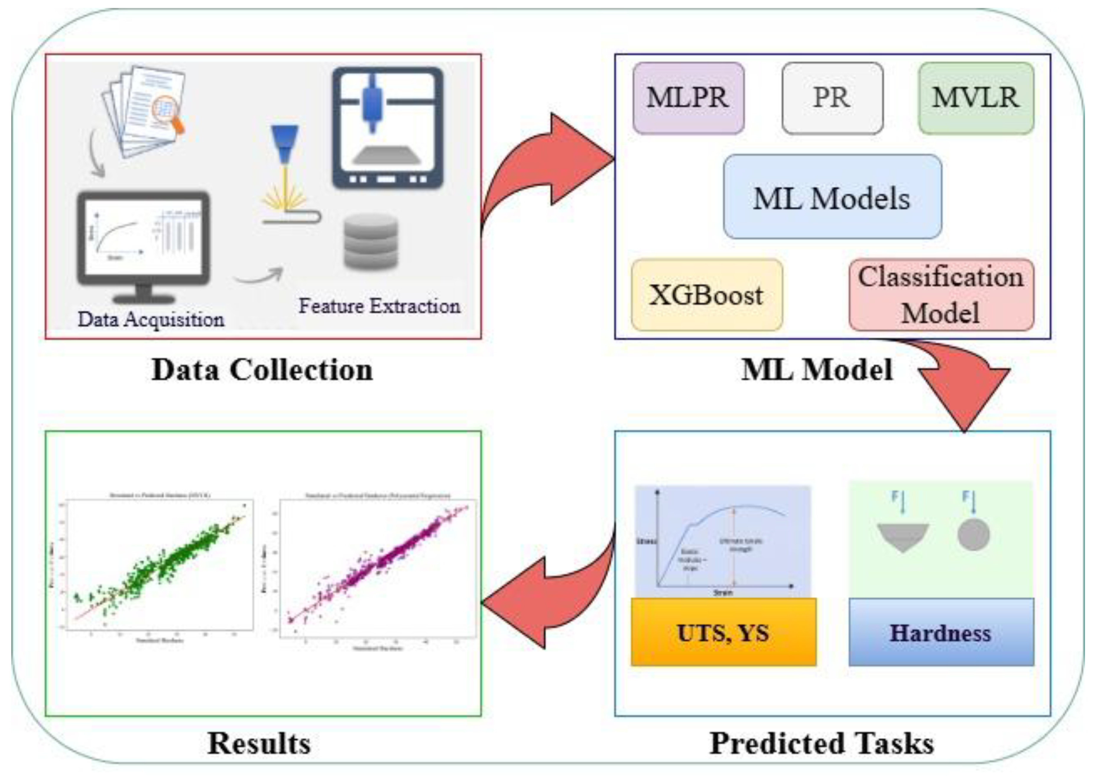
Figure 2.
Featurization strategy used in this study for the ML model training flowchart.
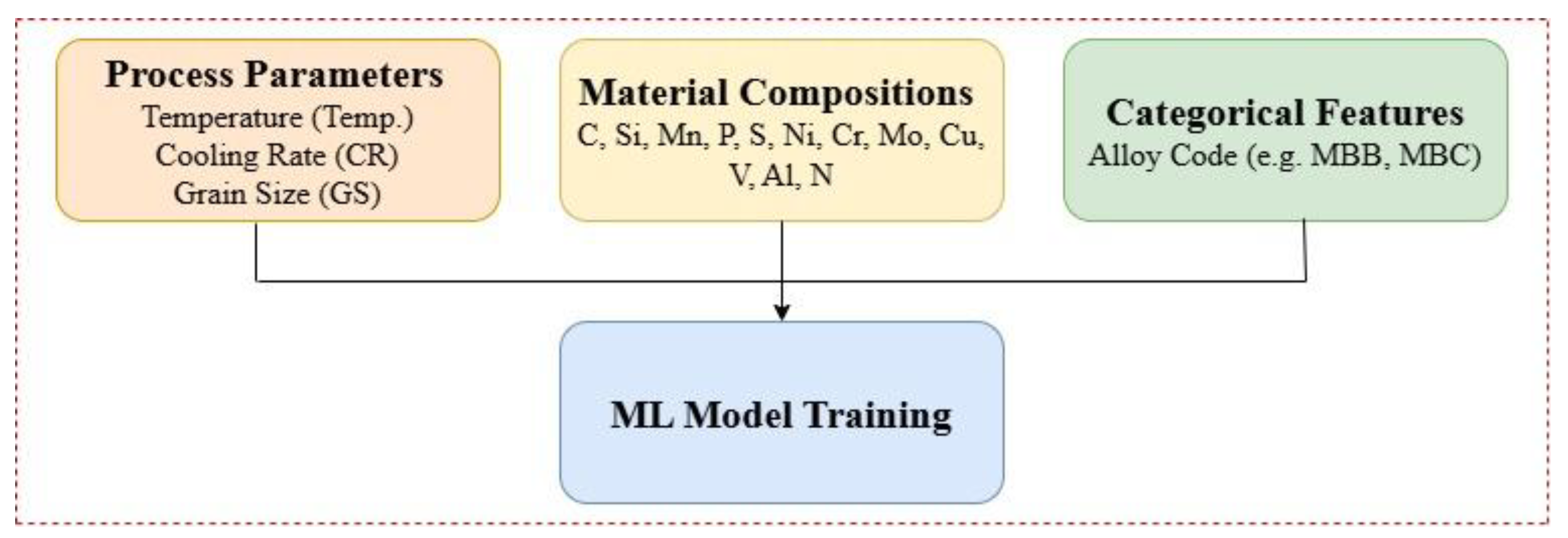
Figure 3.
Comparison of Actual vs Predicted Mechanical Properties-UTS, YS and Hardness Using Various Regression Models Result. (a) to (c) MVLR Model, (d) to (f) PR Model, (g) to (i) MLPR Model, (j) to (k) XGBoost Model.
Figure 3.
Comparison of Actual vs Predicted Mechanical Properties-UTS, YS and Hardness Using Various Regression Models Result. (a) to (c) MVLR Model, (d) to (f) PR Model, (g) to (i) MLPR Model, (j) to (k) XGBoost Model.
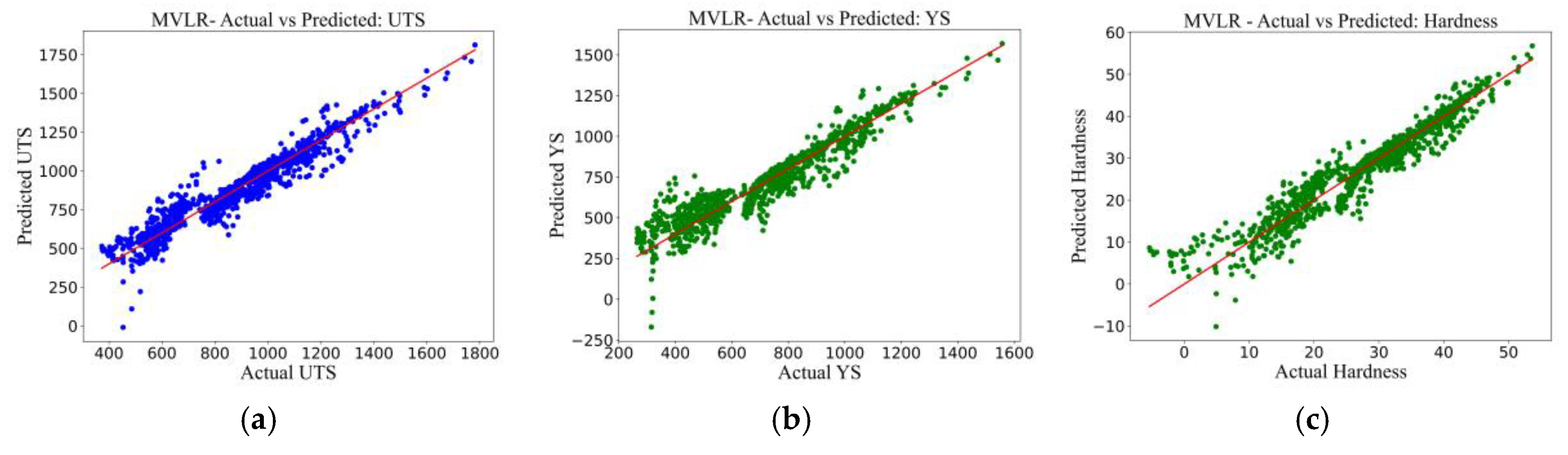

Figure 4.
Residual plots of XGBoost regression model for (a) UTS, (b) YS, and (c) Hardness. The residuals (Actual − Predicted) are plotted against the actual values to assess prediction bias and heteroscedasticity.
Figure 4.
Residual plots of XGBoost regression model for (a) UTS, (b) YS, and (c) Hardness. The residuals (Actual − Predicted) are plotted against the actual values to assess prediction bias and heteroscedasticity.
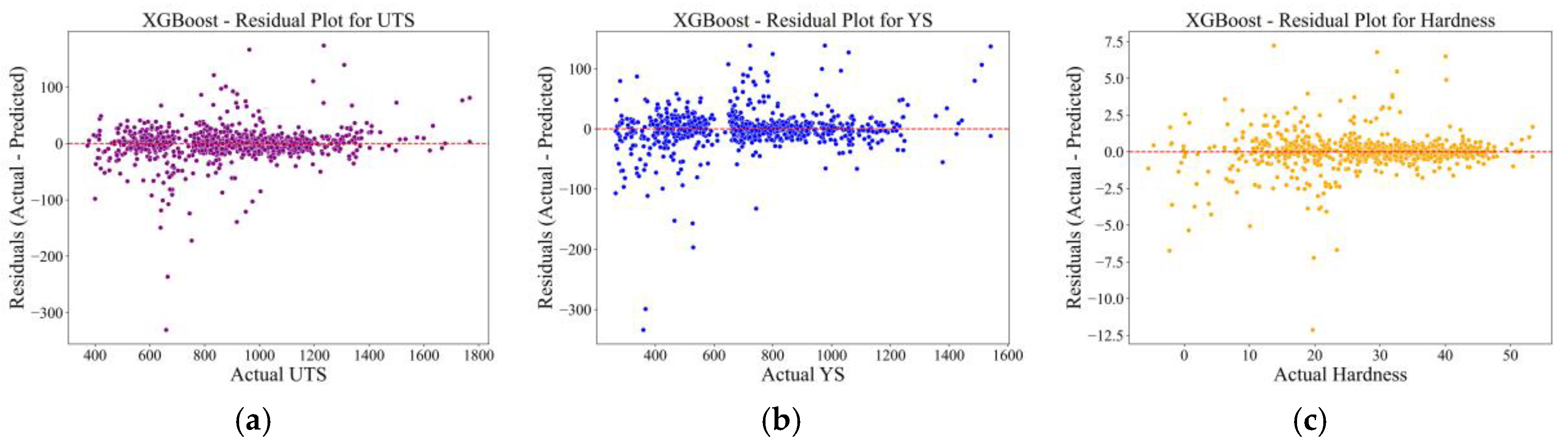
Figure 5.
Distribution of prediction errors (Actual − Predicted) using XGBoost for (a) UTS, (b) YS, and (c) Hardness.
Figure 5.
Distribution of prediction errors (Actual − Predicted) using XGBoost for (a) UTS, (b) YS, and (c) Hardness.
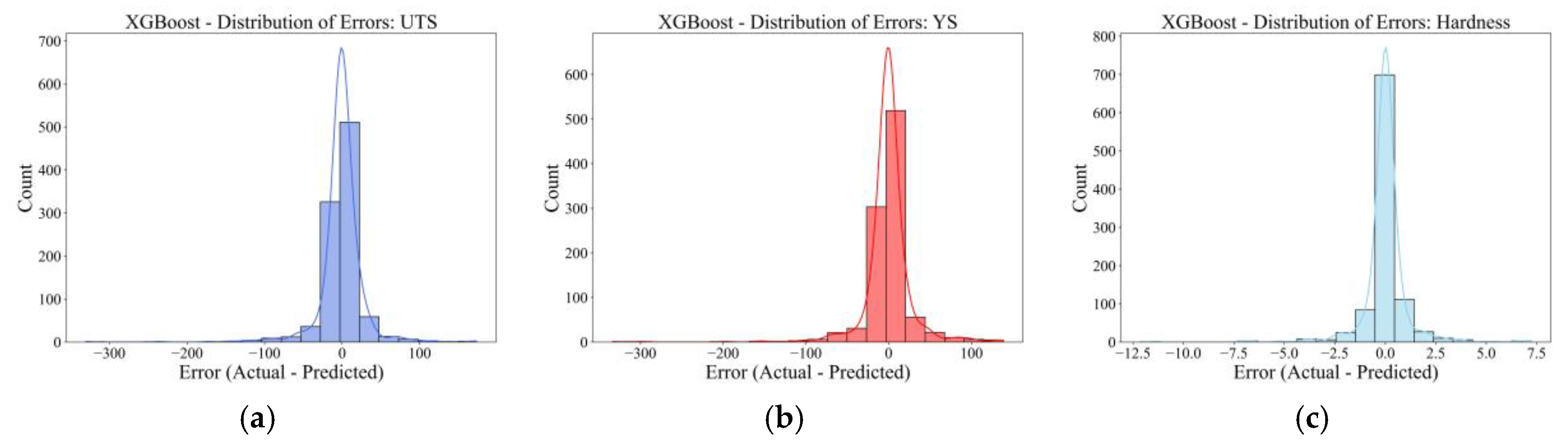
Figure 6.
Confusion matrices for classification model of mechanical property classes using XGBoost model in low alloy steel dataset: (a) Ultimate Tensile Strength (UTS), (b) Yield Strength (YS), and (c) Hardness. The actual vs predicted class labels are categorized as Low, Medium, and High based on value thresholds.
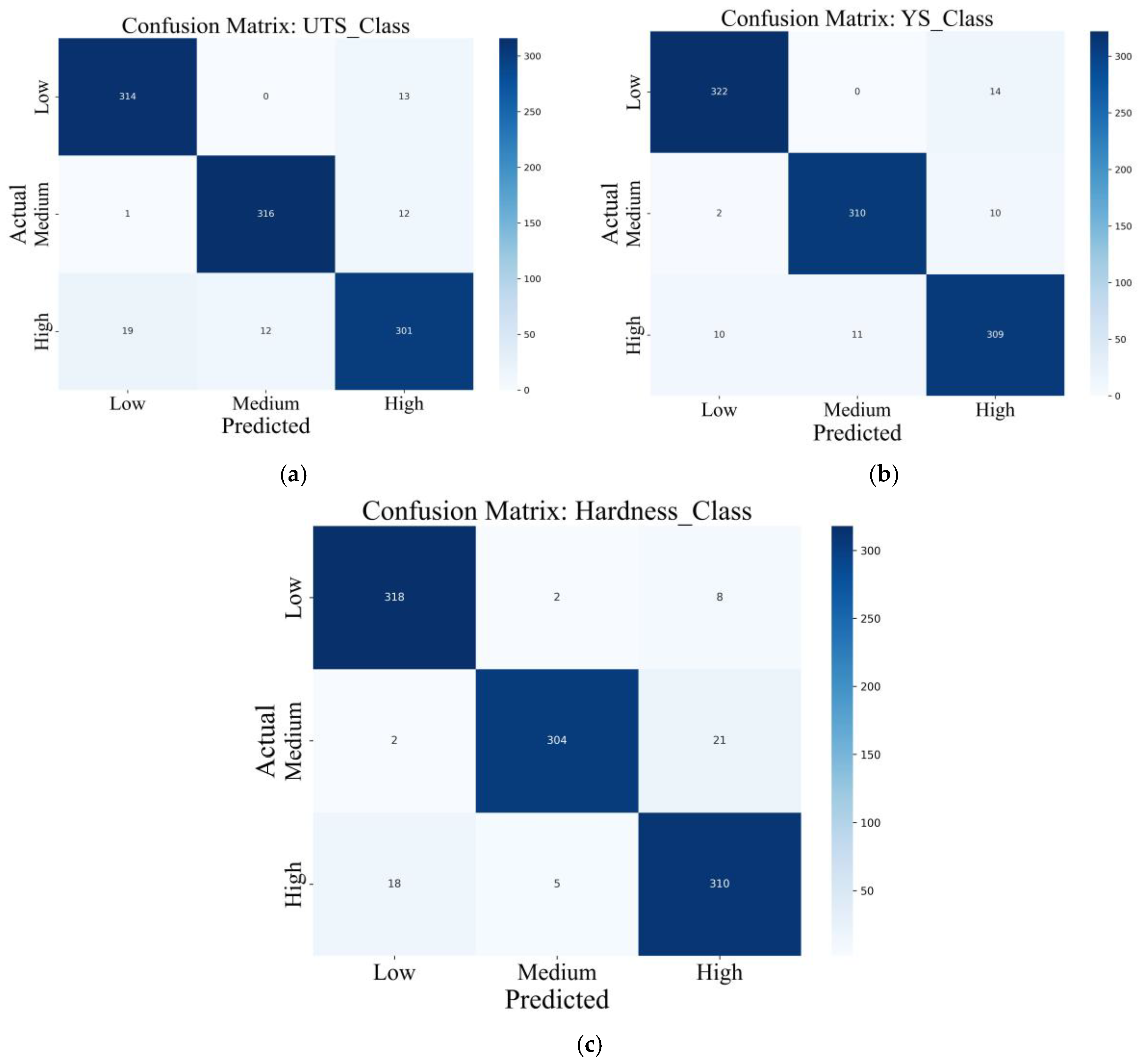
Figure 7.
Pearson correlation matrix among mechanical properties in the low alloy steel dataset.
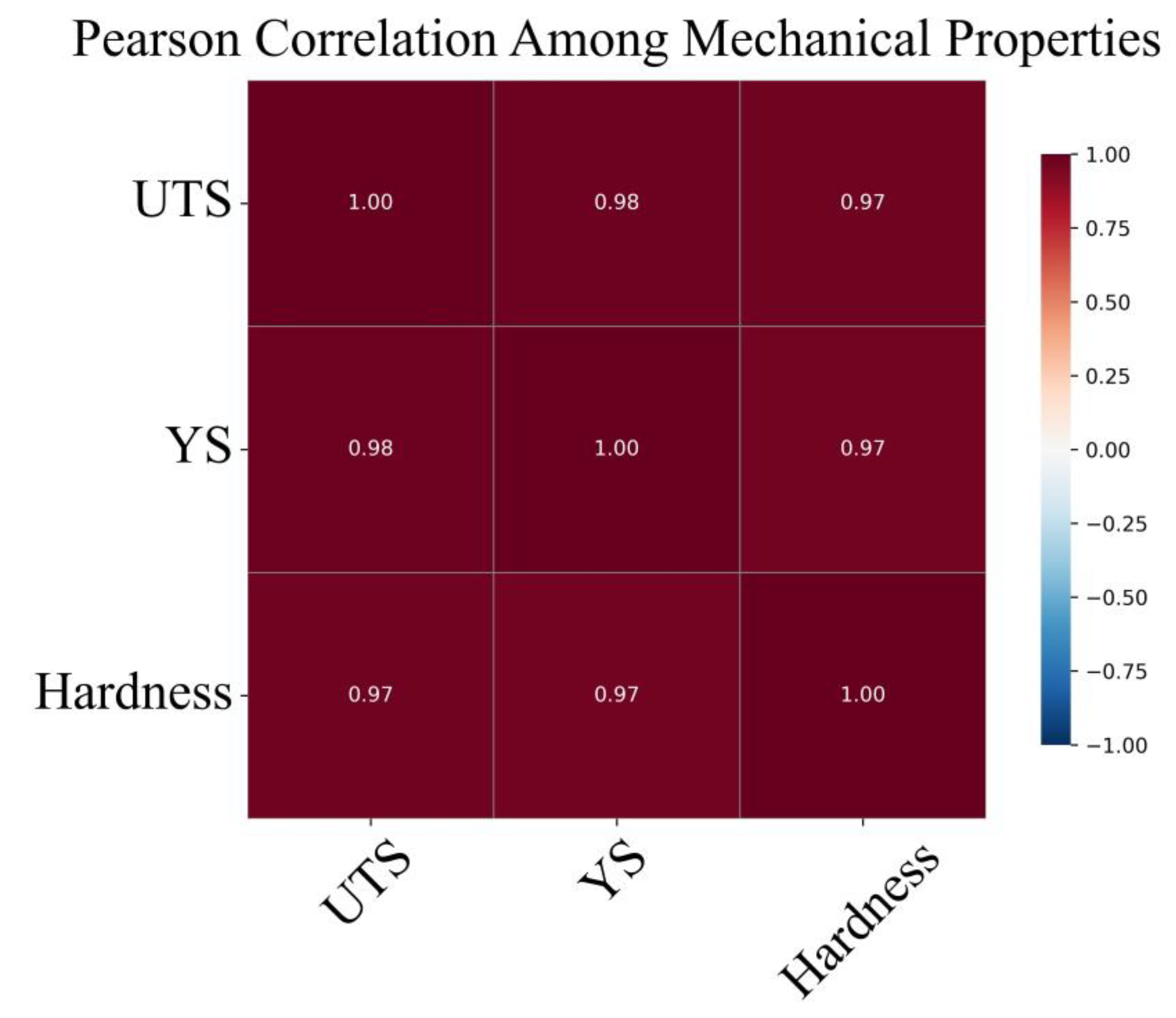
Figure 8.
SHAP features important plots for classification models predicting (a) UTS, (b) YS, and (c) Hardness.
Figure 8.
SHAP features important plots for classification models predicting (a) UTS, (b) YS, and (c) Hardness.
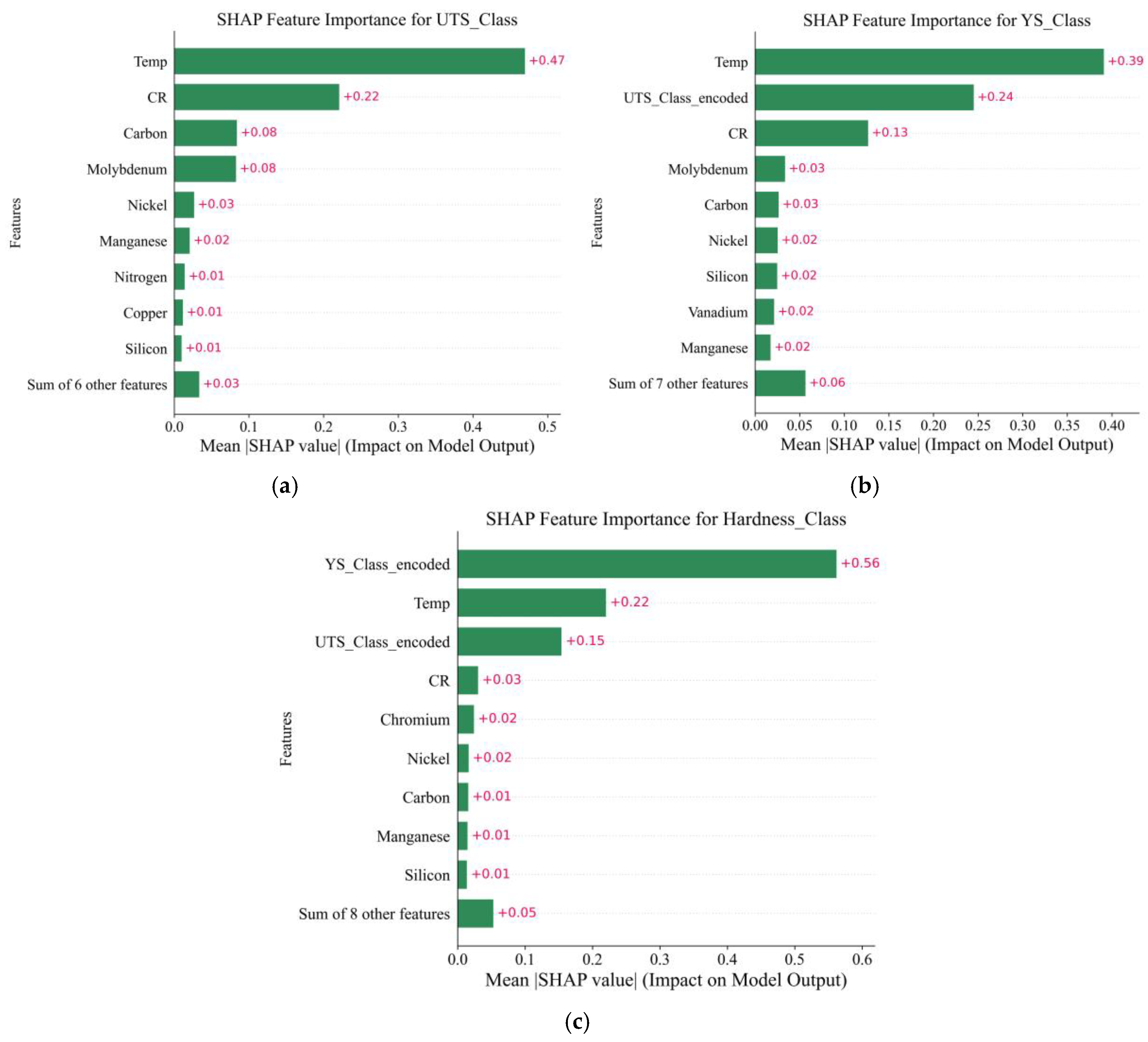
Figure 9.
Drop column feature importance analysis for predicting the low alloy steels dataset (a) Ultimate Tensile Strength (UTS), (b) Yield Strength (YS), and (c) Hardness.
Figure 9.
Drop column feature importance analysis for predicting the low alloy steels dataset (a) Ultimate Tensile Strength (UTS), (b) Yield Strength (YS), and (c) Hardness.
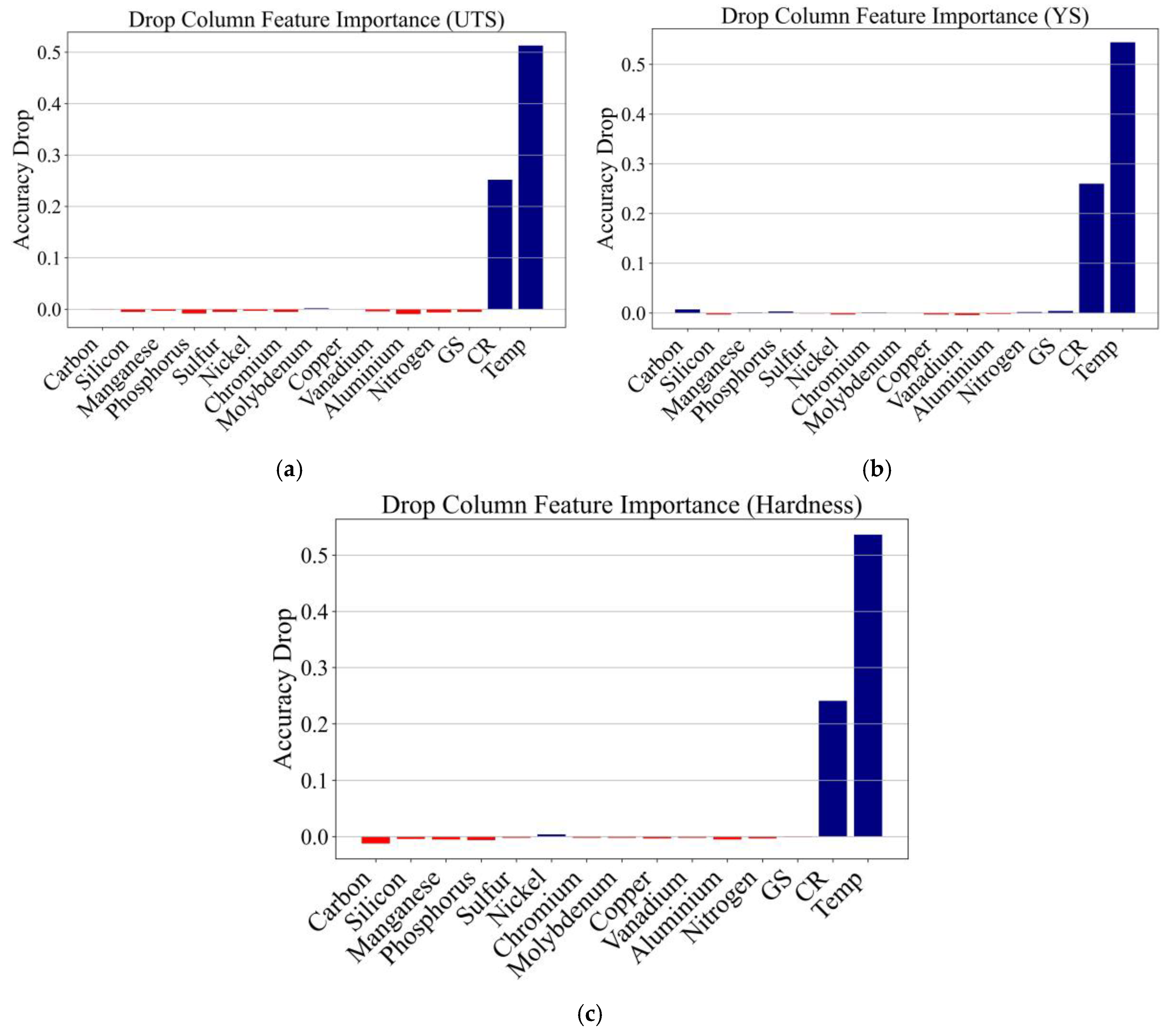
Figure 10.
Multi-Class ROC Curve for low allow steels (a) UTS (b) YS (C) Hardness.
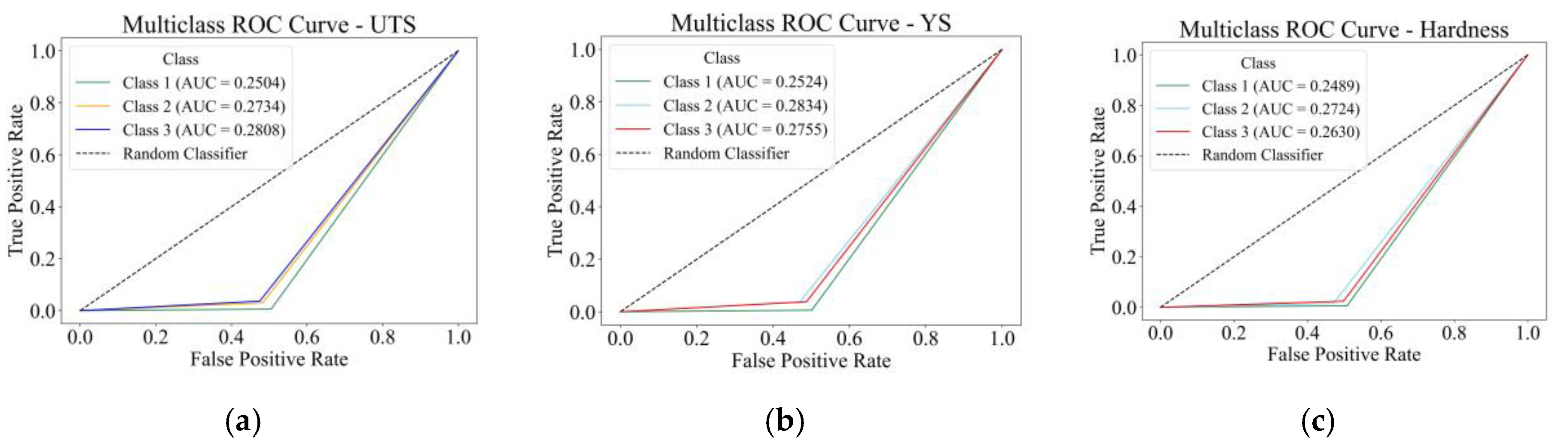
Figure 11.
Multi-Class ROC Curve with AUC for low allow steels (a) UTS (b) YS (C) Hardness.
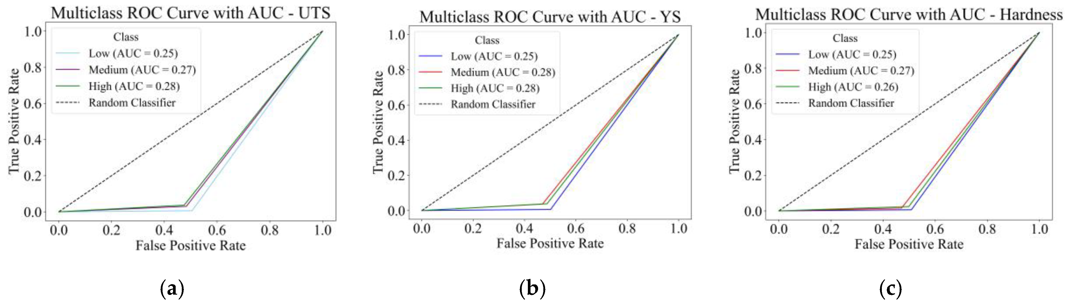

Table 1.
Statistics of the dataset after data cleaning.
| Variables | Description | Min. | Max. | Mean | Median | SD | |
|---|---|---|---|---|---|---|---|
| Input Detector | C | Chemical composition (wt.%) | 0.09 | 0.34 | 0.174 | 0.16 | 0.06 |
| Si | 0.18 | 0.53 | 0.31 | 0.30 | 0.085 | ||
| Mn | 0.42 | 1.48 | 0.797 | 0.66 | 0.342 | ||
| P | 0.006 | 0.03 | 0.015 | 0.014 | 0.005 | ||
| S | 0.003 | 0.022 | 0.01 | 0.01 | 0.004 | ||
| Ni | 0.00 | 0.60 | 0.134 | 0.05 | 0.169 | ||
| Cr | 0.00 | 1.31 | 0.435 | 0.12 | 0.455 | ||
| Mo | 0.005 | 1.35 | 0.451 | 0.50 | 0.387 | ||
| Cu | 0.00 | 0.25 | 0.077 | 0.07 | 0.056 | ||
| V | 0.00 | 0.30 | 0.059 | 0.00 | 0.096 | ||
| Al | 0.002 | 0.05 | 0.012 | 0.006 | 0.013 | ||
| N | 0.0035 | 0.015 | 0.008 | 0.008 | 0.002 | ||
| Grain Size | 20.00 | 20.00 | 20.00 | 20.00 | 0.00 | ||
| Cooling Rate (C/s) | Cooling medium | Categorical | Furnace Cooling-0.01 | Air Cooling-3.3 | Ice Brine-375.00 | ||
| Temperature | 25.00 | 900.00 | 437.37 | 450 | 264.11 | ||
| Output Properties | YS | Yield strength (MPa) | 264.49 | 1557.14 | 728.84 | 727.84 | 244.75 |
| UTS | Ultimate Tensile strength (MPa) | 371.63 | 1781.45 | 878.36 | 876.98 | 244.75 | |
| HV | Hardness Value (HRC) | -5.61 | 53.65 | 28.44 | 29.53 | 10.66 |
Table 2.
MVLR, PR (Degree 2, Degree 3), MLPR, and XGBoost Algorithm Result.
| ML Algorithm | Mechanical Property | MAE | RMSE | R2 |
|---|---|---|---|---|
| MVLR | UTS | 78.86 | 100.9 | 0.82 |
| YS | 79.53 | 104.90 | 0.79 | |
| HV | 3.34 | 4.30 | 0.83 | |
| PR (Degree 2) | UTS | 78.86 | 100.92 | 0.82 |
| YS | 79.50 | 104.90 | 0.79 | |
| HV | 3.34 | 4.30 | 0.83 | |
| PR (Degree 3) | UTS | 50.79 | 71.02 | 0.91 |
| YS | 56.95 | 78.87 | 0.88 | |
| HV | 2.26 | 3.14 | 0.91 | |
| MLPR | UTS | 38.03 | 58.96 | 0.94 |
| YS | 36.94 | 60.65 | 0.93 | |
| HV | 1.68 | 2.67 | 0.93 | |
| XGBoost | UTS | 15.40 | 29.05 | 0.98 |
| YS | 15.43 | 30.17 | 0.98 | |
| HV | 0.5556 | 1.115 | 0.98 |
Table 3.
XGBOOST model summary of Pression, Accuracy, Recall and F1 Score.
| ML Model | Mechanical Property | Pression | Accuracy | Recall | F1 Score |
|---|---|---|---|---|---|
| XGBoost | UTS | 0.9524 | |||
| YS | 0.9524 | ||||
| HV | 0.9676 | ||||
Table 4.
Classification Model Summary of Precision, Accuracy, Recall, and F1 Score.
| Mechanical Property | Class | Precision | Recall | F1-Score |
|---|---|---|---|---|
| UTS | High | 0.95 | 0.96 | 0.95 |
| Low | 0.97 | 0.96 | 0.97 | |
| Medium | 0.92 | 0.92 | 0.92 | |
| Accuracy | -- | -- | 0.95 | |
| Macro Avg. | 0.95 | 0.95 | 0.95 | |
| Weighted Avg. | 0.95 | 0.95 | 0.95 | |
| YS | High | 0.96 | 0.97 | 0.97 |
| Low | 0.96 | 0.96 | 0.96 | |
| Medium | 0.94 | 0.93 | 0.93 | |
| Accuracy | -- | -- | 0.95 | |
| Macro Avg. | 0.95 | 0.95 | 0.95 | |
| Weighted Avg. | 0.95 | 0.95 | 0.95 | |
| HV | High | 0.94 | 0.97 | 0.95 |
| Low | 0.98 | 0.94 | 0.96 | |
| Medium | 0.93 | 0.93 | 0.93 | |
| Accuracy | -- | -- | 0.95 | |
| Macro Avg. | 0.95 | 0.95 | 0.95 | |
| Weighted Avg. | 0.95 | 0.95 | 0.95 |
Table 5.
Cross-Validation Score of Low Alloy Steels Dataset.
| Mechanical Property | K-Fold CV | Stratified K-Fold CV | LOOCV |
|---|---|---|---|
| UTS | 0.99 | ||
| YS | 0.99 | 1.0 | |
| HV | 0.99 | ||
Table 6.
Multiclass Model Result based on the Training and Testing Accuracy.
| Mechanical Properties | Training Accuracy | Testing Accuracy | Model Result |
| UTS | 1.0 | 0.94 | Fit |
| YS | 1.0 | 0.95 | Fit |
| HV | 1.0 | 0.94 | Fit |
Disclaimer/Publisher’s Note: The statements, opinions and data contained in all publications are solely those of the individual author(s) and contributor(s) and not of MDPI and/or the editor(s). MDPI and/or the editor(s) disclaim responsibility for any injury to people or property resulting from any ideas, methods, instructions or products referred to in the content. |
© 2025 by the authors. Licensee MDPI, Basel, Switzerland. This article is an open access article distributed under the terms and conditions of the Creative Commons Attribution (CC BY) license (http://creativecommons.org/licenses/by/4.0/).
Copyright: This open access article is published under a Creative Commons CC BY 4.0 license, which permit the free download, distribution, and reuse, provided that the author and preprint are cited in any reuse.


