
Submitted:
26 March 2025
Posted:
27 March 2025
You are already at the latest version
Abstract
This study evaluates the predictive capabilities of various machine learning (ML) al-gorithms for estimating the hardness of AlCoCrCuFeNi high-entropy alloys (HEAs) based on their compositional variables. Among the ML methods explored, a back-propagation neural network (BPNN) model exhibited superior predictive accuracy compared to other algorithms, including Support Vector Machine (SVM), Stochastic Gradient Descent Regressor (SGDR), Bayesian Ridge (BR), Automatic Relevance De-termination Regression (ARDR), Passive-Aggressive Regressor (PAR), Theil-Sen Re-gressor (TSR), Linear Regression (LR), and Random Forest (RF). The BPNN model achieved excellent correlation coefficients (R²) of 99.54% and 96.39% for training (116 datasets) and testing (39 datasets), respectively. Validation of the BPNN model on an independent dataset (19 alloys) further confirmed its high predictive reliability. Addi-tionally, the developed BPNN model facilitated a comprehensive analysis of the indi-vidual effects of alloying elements on hardness, providing valuable metallurgical in-sights. This comparative evaluation highlights the potential of BPNN as an effective predictive tool for material scientists aiming to understand composition-property rela-tionships in HEAs.
Keywords:
machine learning algorithms
; backpropagation
; artificial neural networks
; high entro-py alloys
; hardness
1. Introduction
High-entropy alloys (HEAs) are a unique class of alloys where multiple principal elements are mixed in relatively high concentrations to maximize the configurational entropy [1]. The HEAs remain a simple solid solution phase, such as face-centered cubic (FCC, using Co, Cr, Fe, and Ni, etc.), body-centered cubic (BCC, using Mo, Nb, Ta, and Zr, etc.), or a mixture of the two instead of forming complex phases and intermetallic compounds [2]. The HEAs possess excellent chemical, and mechanical properties absent in traditional metallic alloys. For instance, the HEAs show high strength, hardness, cryogenic toughness, and thermal stability at elevated temperatures. Further, the alloys resist corrosion and wear [3]. Due to their attractive properties, the alloys have got an immense interest in the scientific community in recent years. Since the HEAs are composed of simple phase constituents (either FCC, BCC, or mixed), the selection of alloying elements has a great influence on mechanical properties.
Due to relatively high amounts of multi-principal elements, the compositions of HEAs are located near or at the center of the composition space [4]. This multi-dimensional compositional space is practically limitless which opens up a vast new realm of alloy design with unprecedented freedom. It comes as no surprise that, even after over a decade only a small fraction of HEAs compositional regions is identified so far within the immense compositional space, and the alloy designing is typically carried out by trial and error methods with low success rate [5]. Hence it is a great challenge to design a search strategy to recognize the desired compositions with some exceptional mechanical properties while minimizing the time and cost-intensive experimentations. In this regard, the progress in computer-aided algorithms with excellent computation capability brings a new opportunity for modelling multicomponent alloy systems [6]. Several novel parameter optimization techniques have been developed to design multivariable complex systems [7]. Especially in the case of HEAs, high throughput CALPHAD [8], high-throughput ab initio method LTVC (for phase identification) [9], DFT, MD (for phase stability, solidification and crystallization kinetics) and genetic algorithms have been developed to accelerate the design of HEAs [10]. However, accurate prediction of the resulting properties for a given combination of constituent elements is crucial to the development and applications of new HEAs. Unlike parametric approaches, machine learning (ML) is a cutting-edge tool that implicit the relations from existing data [11]. The ML method due to its huge success in various fields has become an effective approach and got greater attention in materials science, especially in the HEAs community [12].
Machine learning is a broad computing field where algorithms play a significant role in problem optimization [13]. Several authors reported various ML algorithm types for the optimization of HEAs related issues. For instance, Chang et al. [14] utilized a simulated annealing algorithm (SA) to predict the composition and hardness of HEAs. Menou et al. [15] used a multi-objective optimization genetic algorithm to design the high specific strength HEAs. Therefore, utilizing the best machine learning approach for designing a multi-component system is of great importance. The selection of a proper ML algorithm approach helps to understand the optimum algorithm for designing HEAs with high accuracy as well as high throughput. Several authors used various ML algorithms to design the HEAs, unfortunately, the information regarding the prediction accuracy of train and test datasets, as compared with the other algorithms is often ignored [14]. Finding such information certainly helps the alloy designers to choose a highly accurate ML tool. Comparing the efficiency of various commonly used ML algorithms certainly helps to choose the appropriate ML algorithm for a given problem optimization. However, there is hardly any reported study on this aspect. Considering this, in the present study, we proposed various popular ML algorithms (a total of 9 ML algorithms, namely Support Vector Machine (SVM), Stochastic Gradient Descent Regressor (SGDR), Bayesian Ridge (BR), Automatic Relevance Determination Regression (ARDR), Passive-Aggressive Regressor (PAR), Theil-Sen Regressor (TSR), Linear Regression (LR), Random Forest (RF) and finally the Back Propagation Neural Networks (BPNN)) to predict the hardness of multi-component alloy (Al-Co-Cr-Cu-Fe-Ni) systems. The work mainly concentrated on the AlCoCrCuFeNi alloy system due to its complex phase transitions with alloying as well as limited work availability [16]. In general, the phase formation completely depends on the alloying elements, for example, the CoCrCuFeNi quinary alloying system exhibits only a single solid solution, the FCC phase. On the other hand, the six-elemental alloy, the AlCoCrCuFeNi forms FCC, BCC and a combination of phases according to the alloying content. Thus, the detailed understanding of the alloy behavior with composition is quite complex and challenging, needs significant attention [17]. Therefore, the present study mainly focused on selecting the optimal ML algorithm for understanding the composition-structure-property relationships which helps to design novel multi component AlCoCrCuFeNi alloy systems. The performance of each model was determined with the help of prediction accuracy of both training and testing datasets. Among all ML algorithms, the backpropagation neural networks (BPNN) exhibit a high level of prediction accuracy. Therefore, we utilize the BPNN model to design the new compositions of Al-Co-Cr-Cu-Fe-Ni-based HEAs with excellent mechanical performance.
2. Methods
2.1. Brief Notes on Various ML Algorithms
2.1.1. Support Vector Machine
Support Vector Machine is an ML tool that can be used for regression and classification-based tasks (mainly used for classification). By definition, an SVM constructs a hyperplane or set of hyperplanes in a high or infinite-dimensional space, which can be used for classification or regression. For example, for a given set of input data and predicts, for each given input, two possible classes form the output (binary linear classifier). In the case of the non-linear or higher-dimensional features, the SVM uses different kernel functions where the given non-linear problem is reformulated as a linear problem by different kernel functions [18].
2.1.2. SGD Regressor
SGD is one of the descent tools that has been successfully applied to large-scale ML problems. Simply, it is an iterative method and a very efficient approach for optimizing an objective function. Due to its fast computation and easy learning, the SGD regression is interesting in the research perspective [19].
2.1.3. Bayesian Ridge
The Bayesian ridge regression is a kind of linear regression where the predicted value is considered as a linear combination of the input variable. The method is very useful for process regularization [20]. The method has flexibility in the design for any given problem, however the predictions take noticeably more time to be solved and computed.
2.1.4. Automatic Relevance Determination Regression
ARD regression is a hierarchical Bayesian approach widely used for model selection [21]. The main advantage of the ARD is that the model can be able to switch off the irrelevant input variables (which are irrelevant to the prediction of the output variable) by setting the coefficients to zero. Thus, the model is effectively able to infer which variables are relevant and then switch the others off and prevent the model from overfitting. The method is mainly used where a large number of input variables further allows the irrelevant input variables to be left in the model without harm [22]. A detailed description of ARD regression can be found in [21].
2.1.5. (. e) Passive-Aggressive Regressor
Passive-aggressive algorithms are a family of machine learning algorithms mainly used for both classification and regression. These algorithms can be used for large-scale with regulation parameters [23].
2.1.6. Theil-Sen Regressor
Theil-Sen Regression is a method for robustly fitting a line to sample points in the plane by choosing the median of the slopes of all lines through pairs of points. Due to its simplicity in computation, the method can be applicable for various fields to estimate the trends in the given complex system [24].
2.1.7. (. g) Linear Regression
Regression analysis is one of the most widely used techniques for analyzing multi-factor data. The method is simple and easier to implement and interpret the output coefficients [25]. Diversely, the method over-simplifies real-world problems by assuming a linear relationship among the variables.
2.1.8. Random Forest
Random Forest is a meta estimator that fits several classifying decision trees on various sub-samples of the dataset and uses averaging to improve the predictive accuracy and control over-fitting [23]. Thus, the algorithm builds multiple decision trees and merges them together to get a more accurate and stable prediction. Despite the advantages, the RF has some drawbacks such as much computational power as well as training time.
2.1.9. Backpropagation Neural Networks
Backpropagation is simple, fast and easy to program and is the essence of neural net training. It is a method of fine-tuning the weights of a neural net based on the error rate obtained in the previous epoch. Proper tuning of the weights allows us to reduce error rates and make the model reliable by increasing its generalization. A detailed theory of backpropagation neural networks can be found elsewhere [26].
2.2. Data Processing
The database used in the present study was taken from published literature. A total of 155 combinations of alloy compositions (in at. %) and their respective hardness values [27] were reported in [14]. Overall, the composition of each element varies in vast range and is multi-dimensional.
The minimum, maximum, mean and standard deviation values of each element and hardness values were tabulated in Table 1. The pair plot (or scatter plot matrix) shown in Figure 1 describes the distribution of a single variable and its relationship with all the other variables present in the multi-dimensional variable system [28]. Briefly, the pair plot provides a matrix of the pairwise scatter plots of all variables in the data frame. The principal diagonal of the matrix running from the top left to its bottom right contains the distribution plots or histograms of each variable. Thus, from the pair plot, one can get an idea about the distribution of each variable and the corresponding relation with the other variables present in the database. The data points are randomly distributed and the correlation value (Pearson’s r) between any two given variables is weak and complex. On the other hand, the histogram and the fitted normal distribution curve summarize the distribution of the variable in the database.
3. Results
4.1. Model Development
The composition of the alloy consists of Al, Co, Cr, Cu, Fe, and Ni (in at. %) are considered as the input variables and the hardness [27] is the output variable for constructing the model. The predictive models have been developed with various ML algorithms. Among 155 datasets, 116 datasets were used for training whereas the remaining 39 datasets were used to test the optimal performance of the various ML algorithms. The optimum model for each ML algorithm was determined based on the cross-validation error calculated using Equation 1.
Where Ecve (y)= cross-validation error in prediction of training and testing data set for output parameter y. N = Number of datasets, Ti(y) = Targeted output and Oi(y) = Output calculated.
The cross-validation error during the development of neural networks with the backpropagation ML algorithm is shown in Figure 2. The cross-validation error of training datasets (116) tends to decrease with increasing iterations hence it is quite difficult to find the optimum model with only the training datasets. On the other hand, the cross-validation error of test datasets decreased with increasing iterations at the initial stage and attained a minimum value at 20000 iterations (as indicated in Figure 2). Afterward, the error significantly increased with increasing iterations. Hence, the optimum model was determined based on the minimum test data error.
4.2. Comparing Prediction Accuracy of Various ML Algorithms
The predictive performances of different machine learning (ML) algorithms were compared by examining correlation plots of experimental versus predicted hardness values, as depicted in Figure 3. These plots illustrate the correlation between experimental and predicted hardness values and provide the corresponding correlation coefficient (R²) values for the 39 test datasets. The Passive-Aggressive Regressor (PAR) demonstrated the lowest prediction accuracy, achieving an R² value of only 52.93%. Conversely, both the Support Vector Machine (SVM) and Backpropagation Neural Network (BPNN) models showed excellent predictive performance, each yielding R² values exceeding 90%. Among all the algorithms, the BPNN exhibited the highest accuracy, achieving an R² of 96.39%. For a clearer comparative evaluation, Figure 4 summarizes the R² values of the various ML algorithms for both training (116 datasets) and testing (39 datasets) phases. Based on the correlation coefficients obtained from both datasets, the BPNN model exhibited minimal prediction error and demonstrated outstanding reliability for predicting the hardness of high-entropy alloys (HEAs).
4.3. Validation of BPNN Model
To validate the developed BPNN model we further considered the various HEAs (total of 14 as shown in Table 2) compositions from the literature [7, 20]. The alloy hardness was predicted using the finalized optimal BPNN model. The predicted hardness and respective error values were tabulated in Table 2. The model was able to estimate the hardness values of the validation set of HEAs with considerable accuracy. The average error in the predictions was noted as 18.19. Hence, the developed neural networks model with the backpropagation algorithm could correlate the complex relations among the composition and hardness of HEAs compared with other well-known ML algorithms. Moreover, the BPNN model was able to provide significant prediction accuracy even for validation (unknown) datasets.
4.4. Effect of Element Concentration on the Hardness
The mechanical properties of HEAs strongly depend on the composition and microstructure. D.B. Miracle et al. [30] reported that the alloy composition determines the existing phases and their volume fractions, atomic interactions that influence the properties through the intrinsic properties of the phases. However, the individual elemental effect on hardness values of HEAs is rather limited and only a few studies focused on the variation of individual element amount effect on the mechanical properties of HEAs [31-33]. Therefore, herein with the help of the developed BPNN model, we tried to estimate the effect of alloying elements on the hardness of HEAs. The metallurgical reasoning of predicted hardness results was given, and the results were ensured with the published data. As illustrated in Figure 5a, Al tends to increase the hardness with concentration. As reported in [30,34] the concentration of Al increases, the single-phase FCC (low hardness phase ~ HV 100-200) transforms to BCC+FCC and then to the single-phase BCC/B2 phase which has the higher hardness ranging from HV 500-600. The BPNN predicted trend regarding the variation in hardness as a function of Al content shows close agreement with the experimental trend [39, 42]. As shown in Figure 5b, the effect of Co on hardness is quite negligible yet it tends to minimize the hardness slightly. Qin et al. [35] reported that increase in Co content leads to the formation of the FCC phase which tends to decrease the hardness, and the other possible reason is due to the low solubility of Co in the BCC solid solution the element gets rejected from the high hardness phases and causes a reduction in hardness [36]. In contrast to the Co, the Cr gradually increases the hardness as depicted in Figure 5c. Shun et al. [33] observed that at low concentrations Cr forms the FCC phase and with increasing the Cr content the phase fraction of FCC was decreased, and the element stabilizes the BCC phase. Accordingly, we observed the lowest hardness value at the low content Cr and with increasing Cr, the hardness increased gradually (Figure 5c). The Cu doesn’t show considerable influence on the hardness and the value is almost constant throughout the given range of Cu concentration (0 to 30 at. %) as illustrated in Figure 5d. The estimated behavior of hardness as a function of Fe content is plotted in Figure 5e. From the figure, it is clear that an increase in Fe content leads to a continuous decrement in the hardness and similar results have been reported in the literature [37]. According to Chen et al. [37], the lattice distortion and absence of the Cr3Ni2 phase are the main possible reasons caused by Fe content which results in deterioration of hardness. Finally, the effect of Ni content on hardness is shown in Figure 5f. The Ni tends to increase the hardness in low content levels (< 8 at. %) however, with increasing Ni content leads to decrease the hardness up to 20 at. % and the hardness remained constant with further increase in Ni content. The similar trend of Ni effect has been reported by Suresh et al. [32]. They investigated the effect of Ni content on hardness and found that the higher Ni content (> 10 at. %) significantly decrease the hardness due to the stabilization of single FCC phase. At lower concentrations the increase in hardness is due to the presence of a mixture of both FCC and hard tetragonal phases. Hence, from the estimated results it can be concluded that the develop BPNN model was able to correlate the concentration and hardness of HEAs and provides detailed knowledge regarding the qualitative influence of alloying elements on hardness.

Table 2.
The list of datasets used for validation of the BPNN machine learning model.
| S No | Composition (at. %) | Hardness (Exp.) |
Hardness (BPNN) |
Error | Ref. | |||||
|---|---|---|---|---|---|---|---|---|---|---|
| Al | Co | Cr | Cu | Fe | Ni | |||||
| 1 | 0 | 22.2 | 22.2 | 11.1 | 22.2 | 22.2 | 174 | 160.63 | 13.37 | [7] |
| 2 | 7 | 23.3 | 23.3 | 0 | 23.3 | 23.3 | 125 | 113.68 | 11.32 | [7] |
| 3 | 22.2 | 22.2 | 22.2 | 11.1 | 0 | 22.2 | 564 | 552.28 | 11.72 | [7] |
| 4 | 25 | 0 | 25 | 0 | 25 | 25 | 558 | 517.52 | 40.48 | [7] |
| 5 | 27.3 | 18.2 | 18.2 | 0 | 18.2 | 18.2 | 482 | 462.23 | 19.77 | [7] |
| 6 | 10 | 20 | 20 | 10 | 20 | 20 | 204 | 197.94 | 6.06 | [7] |
| 7 | 33.3 | 16.7 | 16.7 | 0 | 16.7 | 16.7 | 510 | 542.74 | 32.74 | [7] |
| 8 | 18.2 | 18.2 | 18.2 | 9.1 | 18.2 | 18.2 | 563 | 560.96 | 2.04 | [7] |
| 9 | 11.1 | 22.2 | 22.2 | 0 | 22.2 | 22.2 | 160 | 172.77 | 12.77 | [7] |
| 10 | 16.7 | 16.7 | 16.7 | 16.7 | 16.7 | 16.7 | 410 | 409.6 | 0.4 | [7] |
| 11 | 0.5 | 19.9 | 19.9 | 19.9 | 19.9 | 19.9 | 208 | 161.84 | 46.16 | [37] |
| 12 | 19.9 | 0.5 | 19.9 | 19.9 | 19.9 | 19.9 | 473 | 469.61 | 3.39 | [37] |
| 13 | 19.9 | 19.9 | 19.9 | 19.9 | 0.5 | 19.9 | 418 | 407.25 | 10.75 | [37] |
| 14 | 19.9 | 19.9 | 19.9 | 19.9 | 19.9 | 0.5 | 423 | 466.72 | 43.72 | [37] |
4.5. Validation of the Model Predictions with Experimental Results
The composition-property correlations predicted by the BPNN model were validated with the experimental results. Such validation ensures a great degree of confidence in the accuracy of predictions made by the present study. To verify the predicted behavior of hardness, we compared the experimental hardness values of various AlxCoCrCuFeNi alloys. Figure 6 shows the experimentally measured effect of Al content on hardness (shown with a solid red line connecting the triangles) of AlxCoCrCuFeNi where x is varying from 0 to ~40 at.%. It is evident that increasing Al content significantly increases the hardness value (from 130 to 650 HV). On the other hand, the BPNN model predicted hardness values as a function of Al content were denoted with the green-colored circles (Figure 6), and the predicted hardness values were well-matched with the experimental results. The overall experimental and model-predicted hardness values as a function of Al content obey a similar trend. It has been well reported that the properties of HEAs certainly depend on the alloy composition. In particular, the addition of Al can harden the HEAs. This is mainly because of the formation of a hard BCC phase. Initially, the AlCoCrCuFeNi alloy with a lower concentration of Al usually consists of the FCC phase. With increasing the Al content (>10-12 at. %), the formation of the BCC phase can be noticed thus the alloy with a mixture of FCC+BCC reveals higher hardness which further increases with Al content. Finally, the higher Al content (>35 at. %) completely stabilizes the hard BCC phase and raises the hardness values > 700 HV. The variations in the microstructural constituents with increasing Al content in the AlxCoCrCuFeNi HEAs system have been systematically reported in [38,39]. Besides the microstructural variations, the stronger cohesive bonding between Al and other elements and larger atomic size can partly harden the alloy and this phenomenon is generally named as a Cocktail effect [34]. Therefore, the present BPNN model was able to correlate the complex relations that are present among the composition properties of HEAs. More importantly, the predicted behavior follows the experimental trend which certainly helps us to understand the metallurgical phenomenon of other alloying elements that exist in the HEAs. Such clear knowledge about the system helps to design the HEAs with desired properties.
4.6. Significance of Alloy Components on the Hardness
The overall influence of each input variable on the output can be explained with the help of the index of relative importance (IRI). A detailed explanation of this method has been reported in previous studies [40]. The significance of each chemical component on the hardness was represented with the help of a pie chart as shown in Figure 7. According to Figure 7, among all chemical components, the Al shows a positive IRI value (+0.0775) which indicates the element can lead to an increase in hardness value. On the other hand, the Ni exhibits a strong negative impact (with an IRI value of –0.0412) and leads to decline in the hardness value. The order of relative importance of the chemical components on the hardness value of HEAs can be summarized as “Al > Cr > Co > Cu> Fe > Ni”. Therefore, with the help of this method, one can clearly understand the influence of individual components on the hardness.
4. Conclusions
The results of the present work demonstrate that compared to the other ML models, the BPNN method is in good agreement with the predictions for both train and test datasets (99.54% and 96.39%, respectively). According to correlating index values of train and test datasets, the backpropagation ML model can be used as a standalone unit for optimizing the multi-component concentration to achieve better mechanical properties. Furthermore, the model corroborated the hardness values of unknown datasets with considerable accuracy. The graphical user interface was developed to understand the influence of multi-component concentration on hardness which can help to reduce the level of effort required for the experimentation. The model can also be able to provide a huge number of virtual alloy systems within the given range of input variables. Finally, the relative importance index of the components one can utilize to understand the hierarchical order of input variables on the output
Author Contributions
N.S.R. and P.L.N. conceptualized the study. The methodology was developed by P.L.N. and M.I. ANN model Software was developed by N.S.R and P.L.N., while validation was performed by A.K.M. and M.I. Formal analysis was conducted by P.L.N. and M.I., with investigation carried out by A.K.M. and U.M.R. Resources were provided by S.W.C. and N.S.R., and data curation was handled by P.L.N. The original draft was written by U.M.R., A.K.M., and P.L.N., and reviewed and edited by N.S.R. and S.W.C. Visualization was prepared by U.M.R and M.I. The research was supervised by S.W.C. and N.S.R. All authors have read and agreed to the published version of the manuscript.
Funding
This research received no external funding.
Data Availability Statement
All the data is available within the manuscript.
Conflicts of Interest
The authors declare no conflicts of interest.
Abbreviations
The following abbreviations are used in this manuscript:
| BPNN | Back propagation neural network |
| IRI | Index of relative importance |
| HEA | High entropy alloy |
| FCC | Face centered cubic |
| BCC | Body centered cubic |
Appendix A
All appendix sections must be cited in the main text. In the appendices, Figures, Tables, etc. should be labeled starting with “A”—e.g., Figure A1, Figure A2, etc.
References
- George, E.P.; Curtin, W.A.; Tasan, C.C. High Entropy Alloys: A Focused Review of Mechanical Properties and Deformation Mechanisms. Acta Mater. 2020, 188, 435–474. [Google Scholar] [CrossRef]
- Kaufmann, K.; Vecchio, K.S. Searching for high entropy alloys: A machine learning approach. Acta Mater. 2020, 198, 178–222. [Google Scholar] [CrossRef]
- Xie, J.; Zhang, S.; Sun, Y.; Hao, Y.; An, B.; Li, Q.; Wang, C.-A. Microstructure and mechanical properties of high entropy CrMnFeCoNi alloy processed by electopulsing-assisted ultrasonic surface rolling. Mater. Sci. Eng. A 2020, 795. [Google Scholar] [CrossRef]
- Ye, Y.; Wang, Q.; Lu, J.; Liu, C.; Yang, Y. High-entropy alloy: challenges and prospects. Mater. Today 2016, 19, 349–362. [Google Scholar] [CrossRef]
- Lee, S.Y.; Byeon, S.; Kim, H.S.; Jin, H.; Lee, S. Deep learning-based phase prediction of high-entropy alloys: Optimization, generation, and explanation. Mater. Des. 2021, 197. [Google Scholar] [CrossRef]
- Pei, Z.; Yin, J.; Hawk, J.A.; Alman, D.E.; Gao, M.C. Machine-learning informed prediction of high-entropy solid solution formation: Beyond the Hume-Rothery rules. npj Comput. Mater. 2020, 6, 1–8. [Google Scholar] [CrossRef]
- Zhang, Y.; Yang, X.; Liaw, P.K. Alloy Design and Properties Optimization of High-Entropy Alloys. JOM 2012, 64, 830–838. [Google Scholar] [CrossRef]
- Zhang, F.; Zhang, C.; Chen, S.; Zhu, J.; Cao, W.; Kattner, U. An understanding of high entropy alloys from phase diagram calculations. Calphad 2014, 45, 1–10. [Google Scholar] [CrossRef]
- Lederer, Y.; Toher, C.; Vecchio, K.S.; Curtarolo, S. The search for high entropy alloys: A high-throughput ab-initio approach. Acta Mater. 2018, 159, 364–383. [Google Scholar] [CrossRef]
- Rickman, J.M.; Chan, H.M.; Harmer, M.P.; Smeltzer, J.A.; Marvel, C.J.; Roy, A.; Balasubramanian, G. Materials informatics for the screening of multi-principal elements and high-entropy alloys. Nat. Commun. 2019, 10, 1–10. [Google Scholar] [CrossRef]
- J. Schmidt, M.R.G. J. Schmidt, M.R.G. Marques, S. Botti, M.A.L. Marques, Recent advances and applications of machine learning in solid-state materials science. npj Computational Materials 2019, 5, 83. [Google Scholar] [CrossRef]
- Zhou, Z.; Zhou, Y.; He, Q.; Ding, Z.; Li, F.; Yang, Y. Machine learning guided appraisal and exploration of phase design for high entropy alloys. npj Comput. Mater. 2019, 5, 1–9. [Google Scholar] [CrossRef]
- Ishtiaq, M.; Tariq, H.M.R.; Reddy, D.Y.C.; Kang, S.-G.; Reddy, N.G.S. Prediction of Creep Rupture Life of 5Cr-0.5Mo Steel Using Machine Learning Models. Metals 2025, 15, 288. [Google Scholar] [CrossRef]
- Chang, Y.-J.; Jui, C.-Y.; Lee, W.-J.; Yeh, A.-C. Prediction of the Composition and Hardness of High-Entropy Alloys by Machine Learning. JOM 2019, 71, 3433–3442. [Google Scholar] [CrossRef]
- Menou, E.; Tancret, F.; Toda-Caraballo, I.; Ramstein, G.; Castany, P.; Bertrand, E.; Gautier, N.; Díaz-Del-Castillo, P.E.J.R. Computational design of light and strong high entropy alloys (HEA): Obtainment of an extremely high specific solid solution hardening. Scr. Mater. 2018, 156, 120–123. [Google Scholar] [CrossRef]
- Wen, C.; Zhang, Y.; Wang, C.; Xue, D.; Bai, Y.; Antonov, S.; Dai, L.; Lookman, T.; Su, Y. Machine learning assisted design of high entropy alloys with desired property. Acta Mater. 2019, 170, 109–117. [Google Scholar] [CrossRef]
- Singh, S.; Wanderka, N.; Murty, B.; Glatzel, U.; Banhart, J. Decomposition in multi-component AlCoCrCuFeNi high-entropy alloy. Acta Mater. 2011, 59, 182–190. [Google Scholar] [CrossRef]
- Rashidi, A.; Sigari, M.H.; Maghiar, M.; Citrin, D. An analogy between various machine-learning techniques for detecting construction materials in digital images. KSCE J. Civ. Eng. 2016, 20, 1178–1188. [Google Scholar] [CrossRef]
- Pääkkönen, P.; Heikkinen, A.; Aihkisalo, T. Online architecture for predicting live video transcoding resources. J. Cloud Comput. 2019, 8, 9. [Google Scholar] [CrossRef]
- R. Bose, A. R. Bose, A. Das, J. Poray, S. Bhattacharya, Risk Analysis for Long-Term Stock Market Trend Prediction, in: M. Singh, P.K. Gupta, V. Tyagi, J. Flusser, T. Ören, R. Kashyap (Eds.) Advances in Computing and Data Sciences, Springer Singapore, Singapore, 2019, pp. 381-391.
- Mørup, M.; Hansen, L.K. Automatic relevance determination for multi-way models. Journal of Chemometrics: A Journal of the Chemometrics Society 2009, 23, 352–363. [Google Scholar] [CrossRef]
- MacKay, D.J. Probable networks and plausible predictions—a review of practical Bayesian methods for supervised neural networks. Network: computation in neural systems 1995, 6, 469–505. [Google Scholar] [CrossRef]
- Davronov, R.; Adilova, F. A comparative analysis of the ensemble methods for drug design. INTERNATIONAL UZBEKISTAN-MALAYSIA CONFERENCE ON “COMPUTATIONAL MODELS AND TECHNOLOGIES (CMT2020)”: CMT2020. LOCATION OF CONFERENCE, UzbekistanDATE OF CONFERENCE; p. 030001.
- XDang; Peng, H. ; Wang, X.; Zhang, H. Theil-sen estimators in a multiple linear regression model. Olemiss Edu 2008. [Google Scholar]
- Montgomery, D.C.; Peck, E.A.; Vining, G.G. Introduction to linear regression analysis, John Wiley & Sons2012.
- Hassoun, M.H. Fundamentals of artificial neural networks, MIT press1995.
- Varacalle, D.J.; Wilson, G.C.; Johnson, R.W.; Steeper, T.J.; Irons, G.; Kratochvil, W.R.; Riggs, W. A taguchi experimental design study of twin-wire electric arc sprayed aluminum coatings. J. Therm. Spray Technol. 1994, 3, 69–74. [Google Scholar] [CrossRef]
- Sharma, N. Open Data for Sustainable Community: Glocalized Sustainable Development Goals, Springer2020.
- Tung, C.-C.; Yeh, J.-W.; Shun, T.-T.; Chen, S.-K.; Huang, Y.-S.; Chen, H.-C. On the elemental effect of AlCoCrCuFeNi high-entropy alloy system. Mater. Lett. 2007, 61, 1–5. [Google Scholar] [CrossRef]
- Miracle, D.B.; Senkov, O.N. A critical review of high entropy alloys and related concepts. Acta Mater. 2017, 122, 448–511. [Google Scholar] [CrossRef]
- Yeh, J.-W.; Chen, S.K.; Lin, S.-J.; Gan, J.-Y.; Chin, T.-S.; Shun, T.-T.; Tsau, C.-H.; Chang, S.-Y. Nanostructured High-Entropy Alloys with Multiple Principal Elements: Novel Alloy Design Concepts and Outcomes. Adv. Eng. Mater. 2004, 6, 299–303. [Google Scholar] [CrossRef]
- SKoppoju; Konduri, S. P.; Chalavadi, P.; Bonta, S.R.; Mantripragada, R. Effect of Ni on Microstructure and Mechanical Properties of CrMnFeCoNi High Entropy Alloy. Transactions of the Indian Institute of Metals 2020, 73, 853–862. [Google Scholar] [CrossRef]
- Ma, X.; Li, F.; Cao, J.; Li, J.; Sun, Z.; Zhu, G.; Zhou, S. Strain rate effects on tensile deformation behaviors of Ti-10V-2Fe-3Al alloy undergoing stress-induced martensitic transformation. Mater. Sci. Eng. A 2018, 710, 1–9. [Google Scholar] [CrossRef]
- Tsai, M.-H.; Yeh, J.-W. High-entropy alloys: a critical review. Materials Research Letters 2014, 2, 107–123. [Google Scholar] [CrossRef]
- Qin, G.; Xue, W.; Fan, C.; Chen, R.; Wang, L.; Su, Y.; Ding, H.; Guo, J. Effect of Co content on phase formation and mechanical properties of (AlCoCrFeNi)100-Co high-entropy alloys. Mater. Sci. Eng. A 2018, 710, 200–205. [Google Scholar] [CrossRef]
- Kang, M.; Lim, K.R.; Won, J.W.; Na, Y.S. Effect of Co content on the mechanical properties of A2 and B2 phases in AlCoxCrFeNi high-entropy alloys. J. Alloy. Compd. 2018, 769, 808–812. [Google Scholar] [CrossRef]
- Chen, Q.; Zhou, K.; Jiang, L.; Lu, Y.; Lu, Y. Effects of Fe Content on Microstructures and Properties of AlCoCrFe x Ni High-Entropy Alloys. Arabian Journal for Science and Engineering 2015, 40. [Google Scholar] [CrossRef]
- Tong, C.-J.; Chen, M.-R.; Yeh, J.-W.; Lin, S.-J.; Chen, S.-K.; Shun, T.-T.; Chang, S.-Y. Mechanical performance of the Al x CoCrCuFeNi high-entropy alloy system with multiprincipal elements. Met. Mater. Trans. A 2005, 36, 1263–1271. [Google Scholar] [CrossRef]
- Tong, C.-J.; Chen, Y.-L.; Yeh, J.-W.; Lin, S.-J.; Chen, S.-K.; Shun, T.-T.; Tsau, C.-H.; Chang, S.-Y. Microstructure characterization of Al x CoCrCuFeNi high-entropy alloy system with multiprincipal elements. Metall. Mater. Trans. A 2005, 36, 881–893. [Google Scholar] [CrossRef]
- Reddy, N.; Panigrahi, B.; Ho, C.M.; Kim, J.H.; Lee, C.S. Artificial neural network modeling on the relative importance of alloying elements and heat treatment temperature to the stability of α and β phase in titanium alloys. Comput. Mater. Sci. 2015, 107, 175–183. [Google Scholar] [CrossRef]
Figure 1.
Data distribution plots and pairwise relationships among chemical components and hardness. Respective Pearson correlation coefficient r between each pair of variables is mentioned in each plot.
Figure 1.
Data distribution plots and pairwise relationships among chemical components and hardness. Respective Pearson correlation coefficient r between each pair of variables is mentioned in each plot.
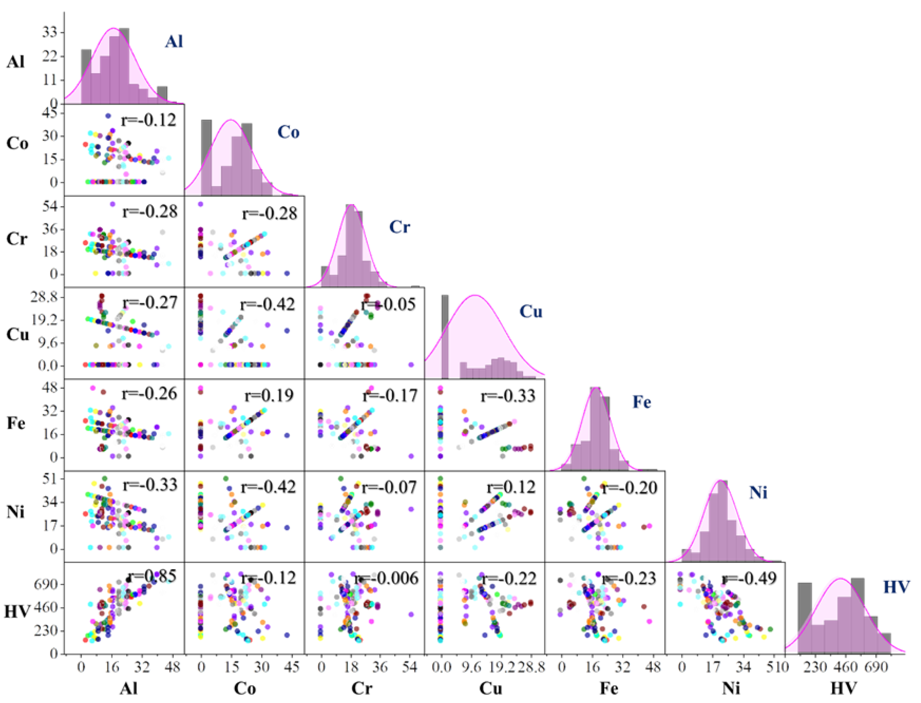
Figure 2.
Change in cross-validation error as a function of iterations in the BPNN model.
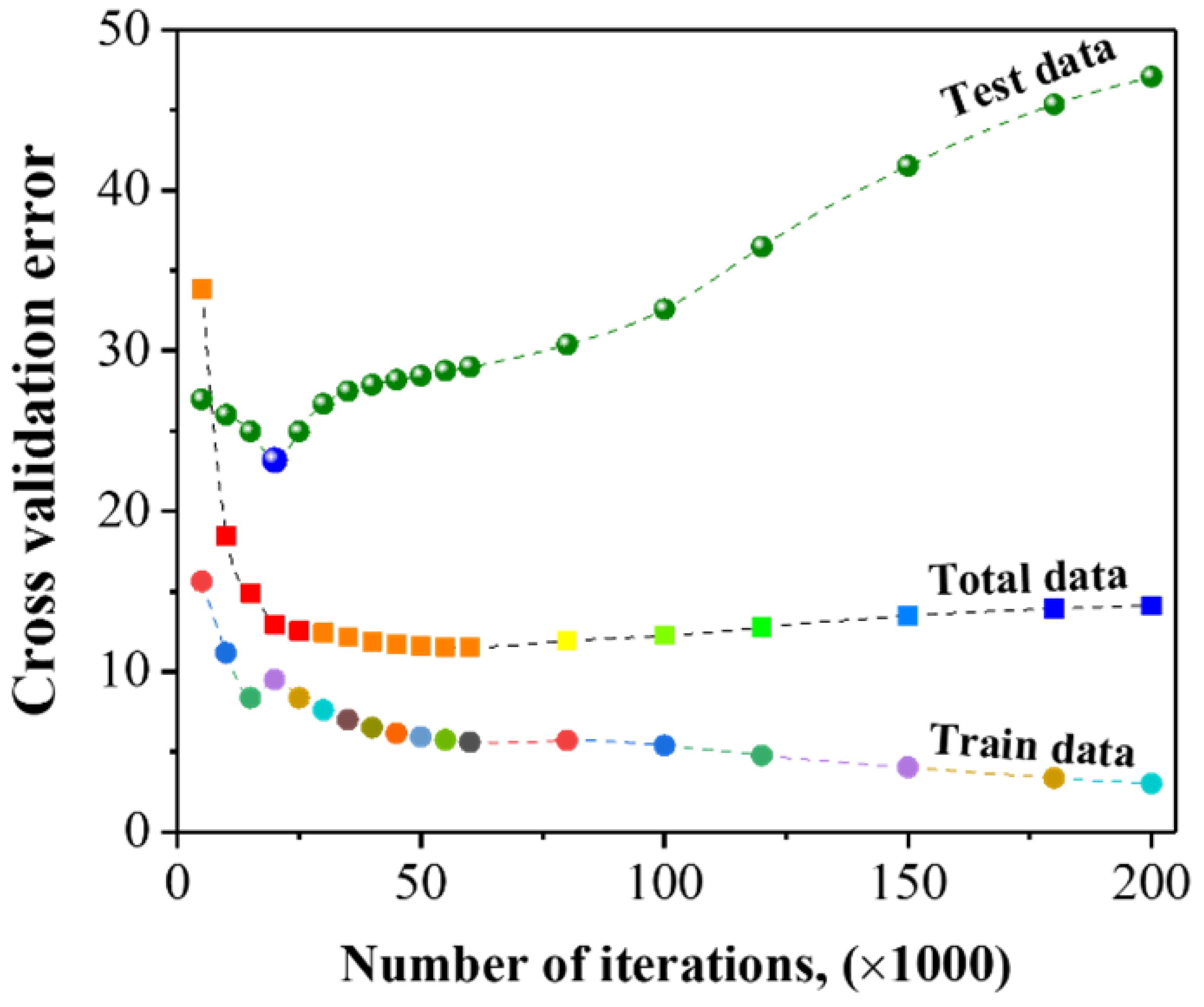
Figure 3.
Performance of various ML algorithms for 39 test datasets.
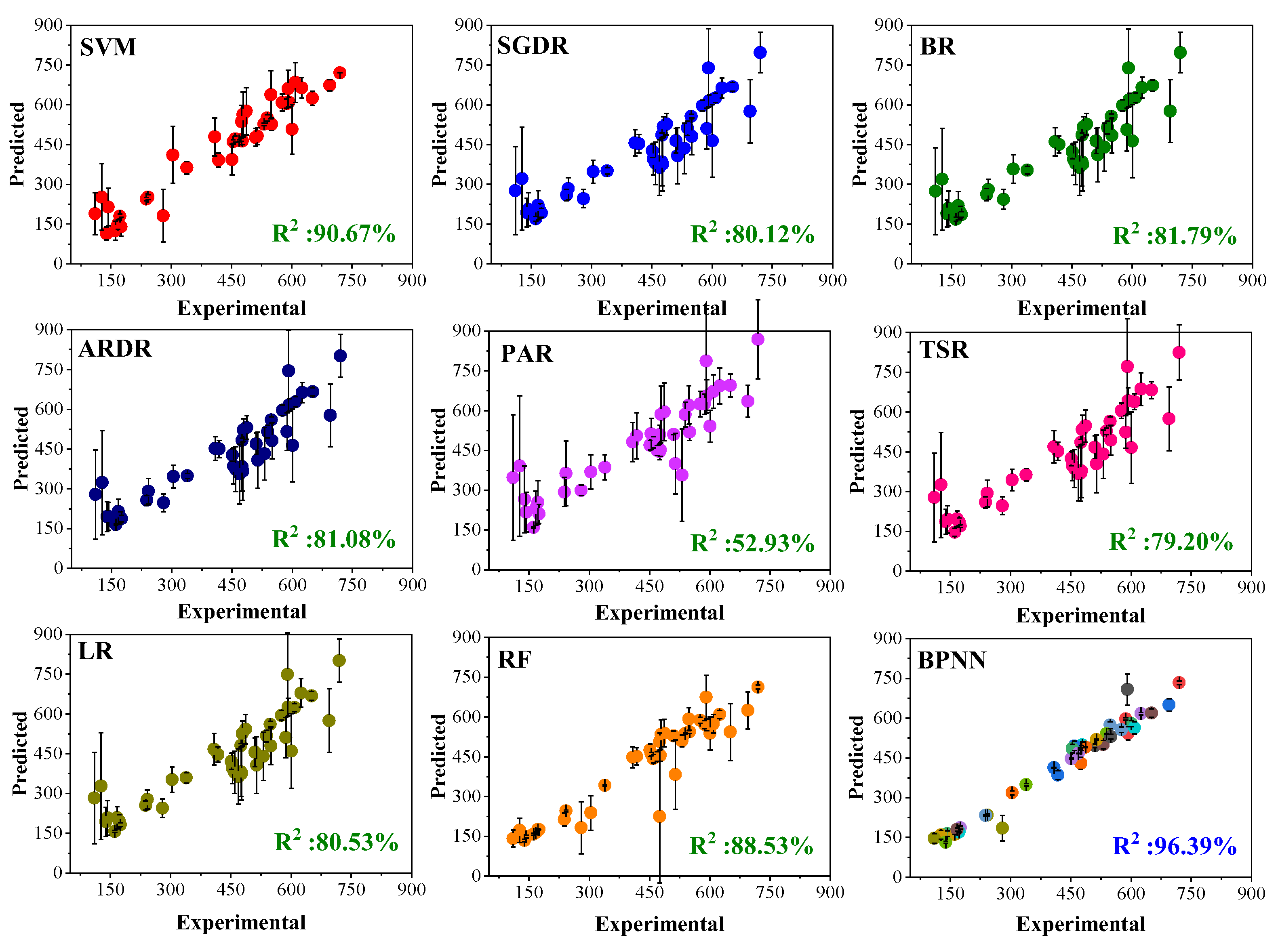
Figure 4.
Correlation coefficient (R2) values of various ML algorithms: (a) train datasets and (b) test datasets.
Figure 4.
Correlation coefficient (R2) values of various ML algorithms: (a) train datasets and (b) test datasets.
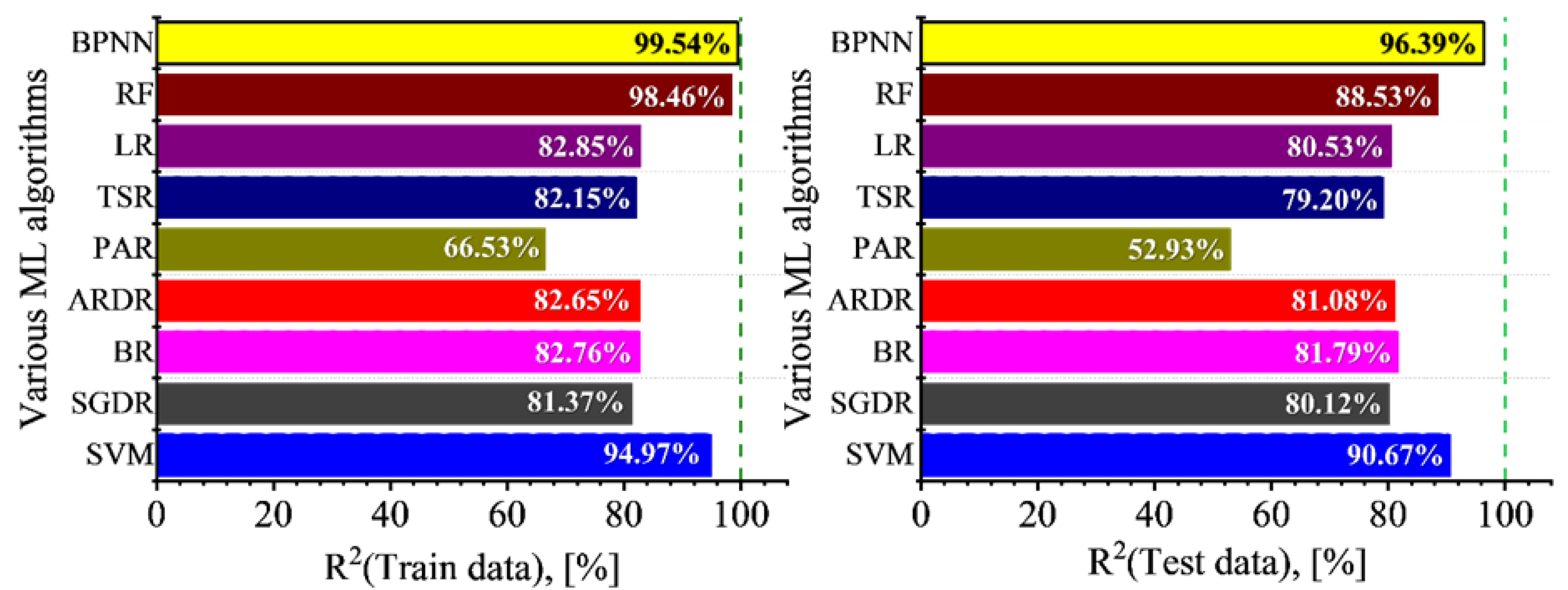
Figure 5.
The BPNN model estimated the results of the element concentration effect on hardness behavior: (a) Al, (b) Co, (c) Cr, (d) Cu, (e) Fe and (f) Ni.
Figure 5.
The BPNN model estimated the results of the element concentration effect on hardness behavior: (a) Al, (b) Co, (c) Cr, (d) Cu, (e) Fe and (f) Ni.
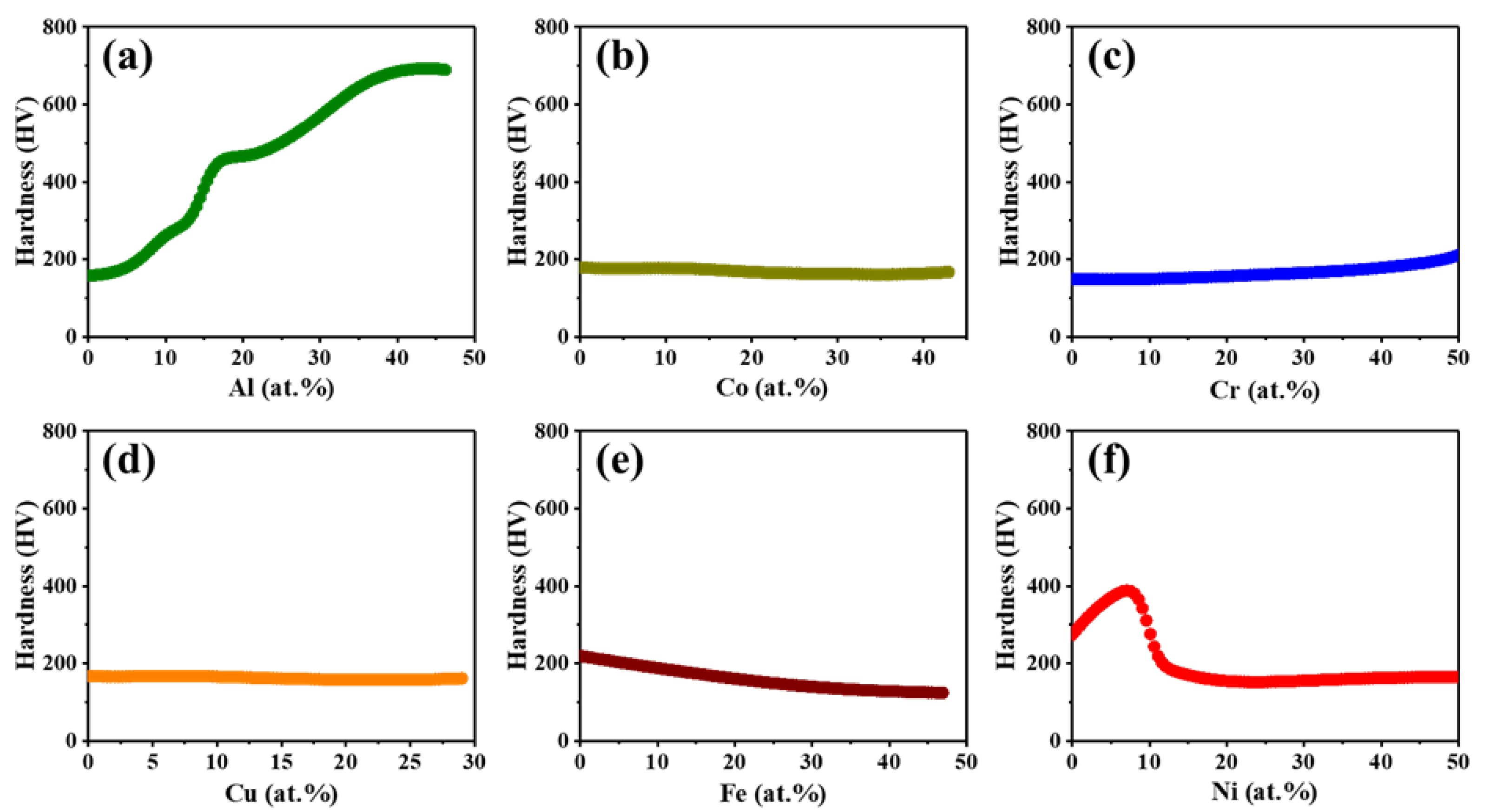
Figure 6.
Comparing the experimental [42] and BPNN model predicted hardness variation trend as a function of Al content in cast AlxCoCrCuFeNi alloys.
Figure 6.
Comparing the experimental [42] and BPNN model predicted hardness variation trend as a function of Al content in cast AlxCoCrCuFeNi alloys.
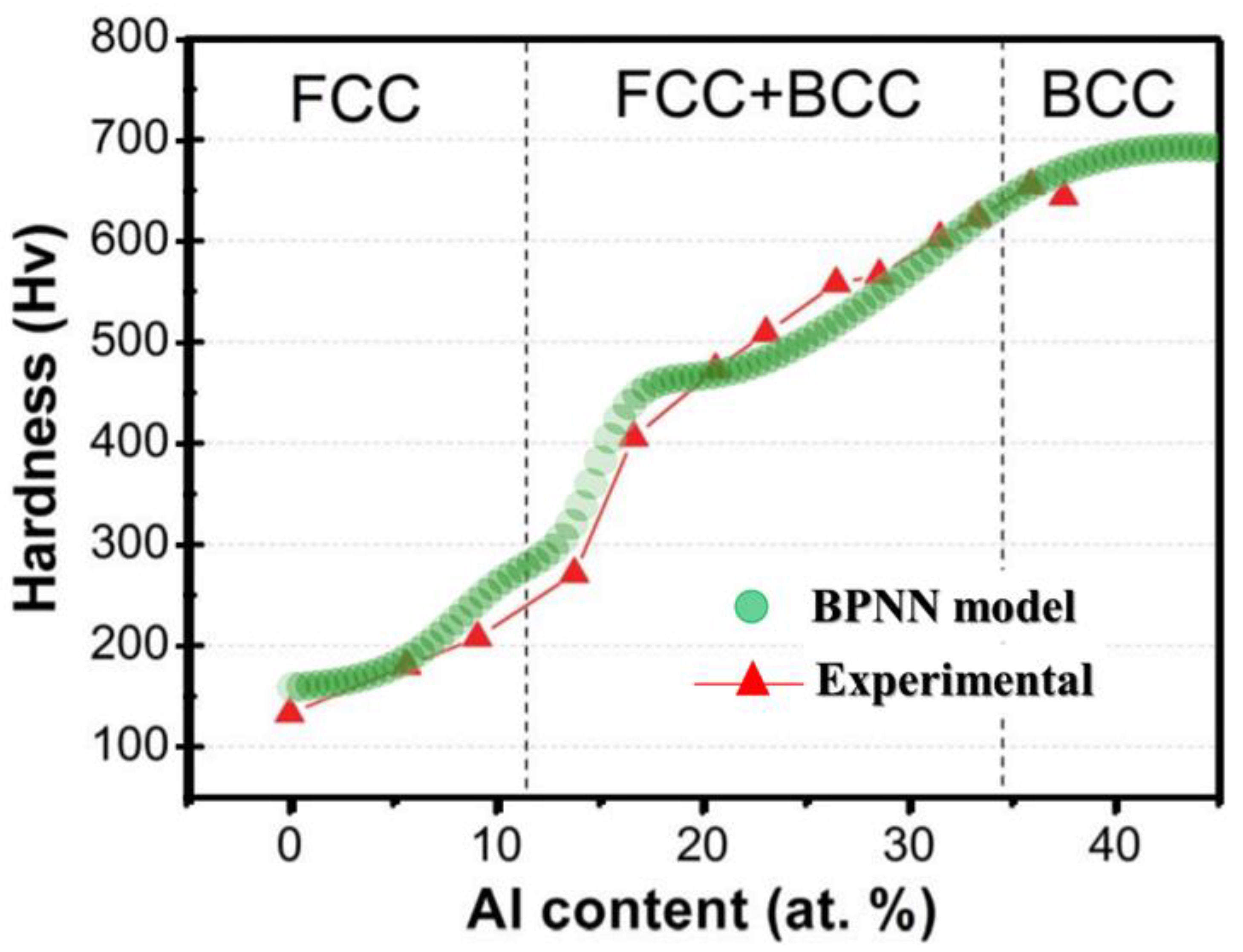
Figure 7.
The significance of chemical components on the hardness of HEAs was estimated using the BPNN model.
Figure 7.
The significance of chemical components on the hardness of HEAs was estimated using the BPNN model.
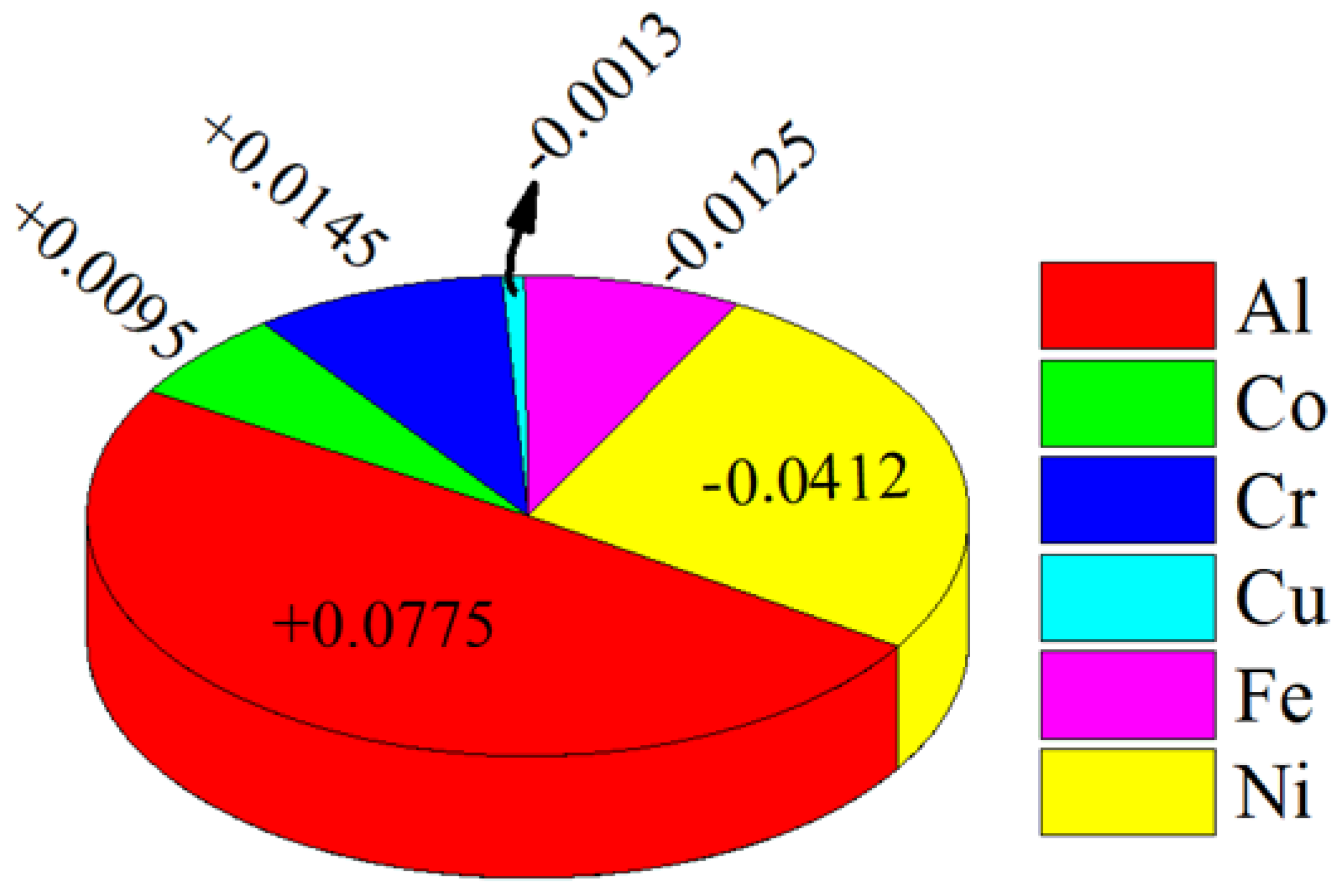
Table 1.
The minimum, maximum, average and standard deviation values of variables.
| Variable | Variables | Minimum | Maximum | Average | Std. Dev. |
|---|---|---|---|---|---|
| Inputs | Al | 0 | 46.2 | 16.89 | 11.26 |
| Co | 0 | 42.9 | 14.56 | 10.23 | |
| Cr | 0 | 55.6 | 18.52 | 8.52 | |
| Cu | 0 | 29 | 10.65 | 9.2 | |
| Fe | 0 | 46.9 | 18.07 | 7.44 | |
| Ni | 0 | 50 | 21.31 | 9.2 | |
| Output | Hardness | 110 | 775 | 422.07 | 187.66 |
Disclaimer/Publisher’s Note: The statements, opinions and data contained in all publications are solely those of the individual author(s) and contributor(s) and not of MDPI and/or the editor(s). MDPI and/or the editor(s) disclaim responsibility for any injury to people or property resulting from any ideas, methods, instructions or products referred to in the content. |
© 2025 by the authors. Licensee MDPI, Basel, Switzerland. This article is an open access article distributed under the terms and conditions of the Creative Commons Attribution (CC BY) license (http://creativecommons.org/licenses/by/4.0/).
Copyright: This open access article is published under a Creative Commons CC BY 4.0 license, which permit the free download, distribution, and reuse, provided that the author and preprint are cited in any reuse.


