
Submitted:
28 January 2025
Posted:
29 January 2025
You are already at the latest version
Abstract
High-entropy alloys (HEAs) have emerged as a novel class of materials that exhibit a wide range of desirable properties making them a focal point for research and potential applications across various industries. The complexity and variability in the compositions of HEAs pose a significant change in predicting their phases, which is crucial for determining their applicability and performance in specific applications. Accurate phase prediction is essential for determining the ideal combination of elements required to design HEAs with targeted properties. This study proposes a machine learning (ML) based approach to predict the phase structure of HEAs utilizing experimental data containing features derived from the chemical composition and corresponding phases. A Boolean vector technique was employed to represent the presence or absence of multiple phase combinations enhancing the model’s ability to accurately capture complex phase structures. Four robust ML algorithms consisting of support vector machine (SVM), k-nearest neighbors (KNN), random forest (RF) and neural network (NN), were employed to develop models capable of classifying the phases of HEAs. The performance of these models was rigorously evaluated through testing on unseen data samples. The findings revealed that both NN and KNN demonstrate superior performance achieving a remarkable test accuracy of 84.85%. This study underscores the potential of ML as an effective tool for predicting the phases of HEAs, offering a new avenue for more innovative approaches to material design and discovery in the future.
Keywords:
high-entropy alloys
; machine learning
; phase prediction
Introduction
High-entropy alloys (HEAs) are a type of metallic alloy that usually contains five or more principal elements in approximately equimolar proportions, as opposed to conventional alloys that typically consist of one or two dominant elements. These alloys are also known as complex metallic alloys or multi-principal element alloys (MPEAs) [1]. The combination of multiple elements in near-equiatomic ratios results unique and superior properties [2] including enhanced corrosion resistance [3,4], high wear resistance [5,6], excellent fatigue resistance [7] and exceptional mechanical strengths [8] that make HEAs the material of choice for a wide range of applications. The burgeoning interest in HEAs is driven by their remarkable attributes which offer new ways to develop of materials with tailored characteristics. The discovery and development of HEAs have opened up exciting possibilities for creating novel materials with customized characteristics and have the potential to revolutionize various industries in the future. The phase structure of HEAs includes Body-Centered Cubic (BCC), Face-Centered Cubic (FCC) and Intermetallic (IM) phases. These phases critically influence the material properties. BCC structures are synonymous with high strength and hardness, while FCC structures enhance ductility and formability. IM phases arising from specific element combinations can enhance or detract from the alloy’s mechanical properties depending on their nature and distribution within the material [9]. Due to the complexity of HEAs’s phase structures, advanced methods are required for phase prediction. Common approaches for predicting phases in HEAs have traditionally relied on trial-and error experimentation. While this method provides essential validation and real-world data, it is often time-consuming and resource-intensive. Consequently, it is challenging to thoroughly explore the extensive compositional space of HEAs using this approach alone. Various empirical design approaches [10,11] have been used to identify the phase formation in solid solution (SS), IM and amorphous (AM) phases. These approaches include parameters such as entropy of mixing (), enthalpy of mixing (), melting temperature (), atomic size difference (), valence electron concentration () and the parameter for predicting solid solution formation (). Additionally, the and electronegativity difference () has been proposed as an empirical rule to differentiate between BCC and FCC structures of SS phases [12]. While these models can indicate certain phase formation trends, their prediction performance is often unreliable, making them not very robust. The Calculation of Phase Diagrams (CALPHAD) [13] and Density Functional Theory (DFT) [14] are efficient computational methods for investigating the thermodynamics and phase stability of HEAs. However, CALPHAD relies on static databases and approximations, which may not fully capture the complexities of systems with higher-order elements [3,15]. On the other hand, DFT does not depend on pre-existing databases, Instead, it computes material properties from first principles. While this allows DFT to avoid the limitations of static data, it demands significant computational resources, making it impractical for modeling disordered or compositionally complex systems such as HEAs [16]. In contrast, machine learning (ML) offers novel and efficient approaches to prediction in material science, providing significant advantages in terms of accelerating the discovery and design of new materials [17,18,19]. This method enables the rapid screening of vast compositional space, predicting material properties based on large datasets. ML has the potential to streamline the discovery and optimization of HEAS by leveraging large, diverse datasets to identify complex patterns and make accurate predictions. Unlike CALPHAD, which relies on static databases with limited flexibility. ML dynamically learns from diverse datasets and can generalize to new compositions, enabling it to handle the complexities of HEAs more effectively. This approach is particularly advantageous given the growing repository of experimental HEA data enabling the development of predictive models that can navigate the complex interplay of compositional and processing parameters to predict phase outcomes accurately.
Several notable recent studies on the application of ML for HEA phase prediction have showcased the efficacy of various algorithms [20,21,22]. The corresponding phase data from experimental observations and some features derived from Gibbs free energy and Hume-Rothery parameters serve as valuable training data for ML algorithms. Islam et al. [23] utilized a neural network (NN) incorporating five input features to categorize phase selection in HEAs as SS, IM or AM. They achieved an average cross-validation accuracy exceeding 80%. Huang et al. [24] proposed ML to effectively investigate phase selection rules using a comprehensive experimental dataset comprising 401 samples. Three diverse ML algorithms: k-nearest neighbors (KNN), support vector Machine (SVM) and neural network (NN) were selected for classifying phases into SS, IM and multiphase SS+IM. The NN achieved the highest testing accuracy of 74.3%. Dai et al. [25] applied six different algorithms consisting of SVM, Ada boost (AB), decision tree (DT), RF, gradient boosting (GB) and logistic regression (LR). They selected 9 initial features and created 36 additional features through dimensionality augmentation. Two distinct feature selection techniques, namely Least Absolute Shrinkage and Selection Operator (LASSO) and Recursive Feature Elimination (RFE), were applied to classify phases as FCC, BCC, Hexagonal close packed (HCP), multiphase (MP) and AM. The findings highlighted that feature engineering led to enhanced predictive accuracy in phase identification compared to conventional methods. Zhang et al. [26] employed NN, SVM and GB and optimized features with feature selection and feature variable transformation based on Kernel Principal Component Analysis (KPCA) to classify phases into SS, IM and SS+IM. The accuracy of the testing set predicted by the SVM was 97.43%. R Machaka et al. [27] trained DT, linear discriminant analysis (LDA), naїve Bayes (NB), generalized linear regression (GLMNET), RF, NN, KNN and SVM to classify solid solution phases into BCC, FCC and BCC+FCC. A total of 36 metallurgy specific features were reduced to 13 features by using feature selection. The RF outperformed the other algorithms with an accuracy rate of 97.5%. Syarif et al. [28] implemented NN to discover the set of element phase formation drivers that can stabilize or destabilize the phase formation of BCC, FCC and IM in HEAs based on the concentration of the alloy constituent element. Nia et al. [29] proposed KNN with an HEA interaction network to categorize FCC, BCC, HCP, MP and AM structures. The results show that the accuracy of the proposed algorithm was 88.88%. Gao et al. [30] employed four ensemble models including RF, XGboost, Voting and Stacking to identify the phases of BCC, FCC and BCC+FCC. Among these algorithms, Voting and Stacking stand out with predictive accuracy of over 92%. He et al. [31] distinguished BCC, FCC, BCC+FCC and AM phases using five ML algorithms. RF showed the best performance of the tested algorithms, with an accuracy of 87%. and parameters play an important role in prediction. The experimental results validated that the phase structure of CoCrFeNiAlx alloys with the increase in Al content is consistent with that obtained by ML prediction. These recent studies highlight ML’s capability not only to achieve high predictive accuracies but also to uncover the underlying phase selection rules that govern the formation of specific phases in HEAs.
Previous research has primarily focused on distinguishing FCC, BCC and FCC+BCC phases in SS [27,30,31] or identifying SS, IM, SS+IM or AM phases [23,24,26]. However, no study has accurately identified complex combinations such as BCC+IM, FCC+IM or BCC+FCC+IM. The current study aims to address this gap by accurately identifying these specific phase combinations in HEAs through the development of a comprehensive model capable of classifying HEAs into a broader spectrum of six distinct phase categories including BCC, FCC, BCC+FCC, BCC+IM, FCC+IM and BCC+FCC+IM. This endeavor not only addresses the intricate challenge posed by multiphase and complex phase structures in HEAs but also makes the following key contributions: (1) introduction of a novel Boolean vector encoding technique to effectively represent complex phase combinations, (2) demonstrating that NN and KNN outperform other models with a maximum accuracy of 84.85% for complex phase predictions, and (3) identification of critical features such as and as major determinants in HEA phase prediction. These contributions collectively enhance the granularity and accuracy of phase prediction, significantly advancing the design and development of HEAs with tailored properties for innovative and cutting-edge applications.
Materials and Methods
Figure 1 illustrates the comprehensive strategy employed in this study to predict the phase structures of HEAs using an ML approach. This strategy encompasses the typical steps of an ML process as applied in materials science [32]. The phase structures considered in this study are categorized into six groups: BCC, FCC, BCC+FCC, BCC+IM, FCC+IM and BCC+FCC+IM.
2.1. Dataset Construction
2.1.1. Data Collection and Feature Extraction
The data for this study were sourced from the existing literature [33,34,35,36,37,38,39,40,41,42,43,44,45,46,47,48,49,50,51,52,53,54,55,56,57,58,59,60,61,62,63,64]. The dataset underwent a manual refinement process which included removing duplicate entries, addressing missing and inconsistent phase data, and limiting the scope to alloys synthesized via arc melting. Alloys produced by different synthesis methods such as powder metallurgy, mechanical alloying, laser melting deposition and additive manufacturing were excluded to avoid the influence of production techniques on the results [9]. After this refinement process, 329 entries remained including 96 BCC, 55 FCC, 52 BCC+FCC, 67 BCC+IM, 46 FCC+IM and 13 BCC+FCC+IM phases. When working with imbalanced datasets, as in this study, careful data handling is crucial to maintain predictive accuracy. To address this, a Boolean vector approach was introduced. In cases where multiple phase combinations need to predicted, a Boolean vector can represent each phase as a separate binary outcome. This enables the model to focus on learning which elements or conditions are associated with each phase combination individually rather than struggling to learn from an uneven distribution across multiple overlapping classes [65]. The corresponding phases were encoded with three entries corresponding to {BCC, FCC, IM} phases as shown in Table 1. A value of 0 indicates the absence and 1 indicates the presence of a specific phase. The logical values in the target variable indicated the set of phases present in each HEA sample. For instance, [1,0,0] represents BCC, [1,1,0] represents BCC+FCC and [1,1,1] represents BCC+FCC+IM.
The dataset comprises numerical features derived from the chemical composition of the alloys and their corresponding phases. Seven features were extracted from the chemical composition of each entry using the equations presented in Table 2. These features were , , , , , and . These calculated features provide essential information for the ML models to understand the underlying relationships in the alloy compositions enabling the prediction of phase structures with greater accuracy.
2.1.1. Data Normalization
Preprocessing data in ML is an essential step to enhance data quality and ensure their suitability for ML algorithms. One common technique is normalization which standardizes the range of feature data, ensuring that each feature contributes approximately equally to the final prediction as described by the following formula:
where is the standardized value of the feature, is the original value of the feature, is the mean value of the feature and is the standard deviation of the feature. The purpose of normalization is to produce dimensionless numerical features so that each data point is on the same numerical scale. This process is crucial for improving the accuracy of the ML model by ensuring that no single feature dominates the learning process due to its scale.
2.2. ML Algorithms
ML algorithms have become a power tool for predicting complex material properties including the phase structure of HEAs. By leveraging large datasets and sophisticated algorithms, researchers can identify patterns and relationships that traditional methods may overlook. In this study, four ML algorithms were employed to predict the phases of HEAs: SVM, KNN, RF and NN. These algorithms were implemented using the scikit-learn library and were selected based on their frequent application in similar studies and their demonstrated effectiveness in handling classification tasks in material science. Each algorithm offers unique strengths: SVM excels in distinguishing non-linear relationships, KNN is simple yet effective for pattern recognition, RF is robust against overfitting and interpretable due to feature importance analysis, and NN is well-suited for capturing complex, non-linear interactions within the dataset.
- Support Vector Machine (SVM)
The SVM aims to find the hyperplane that best separates different classes of data points. This separation is achieved by minimizing the loss function which involves finding the hyperplane that maximizes the margin between the classes. It can handle nonlinear boundaries by using the Kernel function [68,69]. the Kernel function transforms the data into a higher dimensional space where separation might be possible. The key hyperparameters used for the SVM in this study are penalty (C), the Kernel function and the Kernel coefficient (gamma). When C is too large, the model may overfit the training data, leading to poor generalization to new data. When C is too small, the model might not capture outliers well resulting in high training set errors and limiting to fit the training data. Different Kernel functions serve different purposes and can capture various types of relationship in the data. The Radial Basis Function (RBF), Polynomials, and Sigmoid Kernels are Kernel functions used for the SVM in this study. Gamma affects the sensitivity to differences in feature vectors. If gamma is set too high, the model might overfit as it would become sensitive to individual data points. If gamma is chosen too low, the model may not capture the underlying patterns in the data.
- K-Nearest Neighbor (KNN)
The KNN makes predictions based on the minimum distance between data points and a simple majority vote from the nearest neighbors. Its hyperparameters are the number of neighbors to consider for prediction, the weight function, the algorithm for computing the nearest neighbors and a distance metric [29,70]. Smaller values of nearest neighbors can make the model sensitive to noise, while larger values can make it biased. For this study, two common weight function options are uniform (equal weights) and distance (inverse of distance as weight). The algorithms used for efficiently computing the nearest neighbors are Auto, ball tree, KD tree and brute force. Euclidean and Manhattan are used to measure the distance between data points.
- Random Forest (RF)
RF is an ensemble technique that combines multiple decision trees to make predictions. Each tree relies on values from a random vector sampled independently and from the same distribution for all trees. The majority predicted class across trees become the final predicted class. The hyperparameters for tuning this model include the number of trees, the maximum feature, the maximum tree depth, the minimum sample split, the minimum sample leaf and bootstrap sampling. The number of trees determine the decision tree in the forest. Increasing the number of trees can improve model performance, but it also increases computation time. The maximum feature specifies the maximum number of features considered for splitting a node in each decision tree. This parameter can impact the diversity and randomness of the trees, reducing overfitting. The maximum tree depth defines the maximum number of levels a decision tree can have. Restricting tree depth can help prevent overfitting and enhance generalization. The minimum sample split sets the minimum number of data points required in a node before it is eligible for further splitting. The minimum sample leaf specifies the minimum number of data points that a leaf node must contain. If bootstrap sampling is set to true, sampling is performed with replacements when constructing individual decision trees [68].
- Neural Network (NN)
The NN is a type of feedforward neural network with multiple layers including an input layer, one or more hidden layers and an output layer. The key hyperparameter associated with training the NN are number of the hidden layers, size, activation functions, the loss function, the optimizer and the learning rate. The number of hidden layers and the number of neurons in each hidden layer are crucial parameters which define the depth and width of the neural network. More layers and neurons allow the network to capture more complex patterns but also increase the risk of overfitting and the computational complexity [71]. Activation functions like rectified linear unit (ReLU), sigmoid or tanh are used to introduce nonlinearities in the model, allowing it to learn more complex relationships. Different activation functions have different properties and are suitable for different types of data. The loss function is a measure of how well the neural network is performing. The optimizer is an algorithm that adjust the weights of the network to minimize the loss. Common optimizers include stochastic gradient descent (SGD), adaptive moment estimation (Adam), etc. The learning rate is a hyperparameter that controls how to change the model in response to the estimated error when the model weights are updated. A small value can make the training process very slow while a large value can cause the model to converge too quickly to the optimal solution or even diverge.
Table 3 summarizes the hyperparameter options and their ranges for the SVM, KNN, RF and NN used for the phase prediction of HEAs in this study. Each hyperparameter is crucial for tuning each model to achieve optimal performance. The dataset was randomly divided into two subsets at an 80:20 ratio for training and testing. This means that 80% of the data were used to train the models while the remaining 20% were reserved for testing the model performance. This split helps ensure that the models are trained on a comprehensive portion of the data while also providing an unbiased evaluation of their performance on unseen data. To prevent overfitting where a model performs well on the training data but poorly on new data, a cross-validation (CV) technique was employed during the model training process. In five-fold CV, the training data are divided into five subsets. The model is trained on four of these subsets and validated on the remaining subset. This process is repeated five times, each time with a different subset used for validation [72]. The results are then averaged to provide a more accurate estimate of the model’s performance. This method ensures that the model generalizes well to new data, improving its robustness and reliability.
2.3. Evaluation of Model Performance
During model training, five-fold CV was applied to assess the mean CV accuracy of each model, providing an initial measure of model reliability and generalizability. For testing with an unseen dataset, multiple evaluation metrics were calculated to provide a comprehensive performance assessment. These metrics included accuracy, precision, recall and F1-score. Accuracy measures the ratio of correctly predicted instances to total instances. Precision calculates the proportion of true positives among all predicted positives. Recall assesses the model’s ability to identify all true positives. F1-score combines precision and recall to find their harmonic mean for a balanced assessment. These metrics are defined as follows [73]:
Where a true negative () is an instance that is actually negative and correctly predicted as negative, a true positive () is an instance that is actually positive and correctly predicted as positive, a false positive () is an instance that is actually negative but incorrectly predicted as positive and a false negative () is an instance that is actually positive but incorrectly predicted as negative. Additionally, the Receiver Operating Characteristic (ROC) curve and the Precision-Recall (PR) curve were analyzed to provide a better understanding of model performance. The ROC curve provides insight into the trade-off between the true positive and false positive rate, while the PR curve highlights the balance between precision and recall, which is especially valuable for assessing models on imbalanced datasets.
The complex combination phase prediction accuracy offers a rigorous evaluation standard for applications requiring precise phase identification in HEAs. This metric along-side the other performance indicators, provides a comprehensive overview of each model’s suitability for predicting HEA phase compositions in both individual and multi-phase scenarios.
3. Results and Discussion
3.1. Data analysis
The pair plot generated using the Seaborn library, as depicted in Figure 2, showcases the relationships between pairs of features. Each scatter plot point corresponds to a specific phase in the dataset, with its position representing the values of the two features for that phase. The diagonal cells contain Kernel density plots illustrating the distribution of each individual features. The pair plot reveals that certain feature pairs, such as and exhibit noticeable trends, where specific phase categories cluster within distinct regions. For instance, FCC phases tend to align with higher VEC values, while BCC phases correlate with lower values and more negative . These relationships indicate that some features play a critical role in determining phase stability and composition, offering valuable insights for phase prediction.
The radar plot in Figure 3 provides a comparative visualization of the normalized feature values for each phase category. The plot highlights distinct patterns across the phases, with BCC phases exhibiting lower values and higher while FCC phases show relatively higher values. IM phases, on the other hand, demonstrate a unique combination of high and more negative , reflecting their ordered structures and complex bonding characteristics. These differences emphasize the significance of these features in distinguishing between phase categories
Figure 4 shows a heat map illustrating the relationships or correlations between feature in the dataset. Each cell in the matrix represents the correlation coefficient between two features, ranging from -1 to 1. A value of 1 indicates a strong positive correlation, -1 indicates a strong negative correlation and 0 indicates no correlation between features. The values in the heatmap are correlation coefficients which measure the strength and direction of the linear relationship between two features. The most commonly used correlation coefficient is the Pearson correlation coefficient calculated as follows:
where is the Pearson correlation coefficient between feature and . and are the individual sample points indexed with . and are the means of the and features, respectively.
The correlation values in heat map of two independent features range from -0.75 to 0.58. Specifically, and exhibit a negative correlation implying that as increases, tends to decrease. Higher values favor FCC structures whereas lower values stabilize BCC structures, since FCC phases often have lower . Conversely, the electronegativity difference and show a positive correlation, meaning that as increases, so does the melting temperature. Larger values can promote the formation of complex phases or IM phases which often have higher than SS phases [74]. Overall, there are no strong positive or negative correlations between the features. Thus, all the features can be retained.
The 3D scatter plot was created to illustrate the phase distribution across three axes: , and . The relationship between these features and the corresponding phases is displayed in Figure 5. From the plot, it is apparent that IM phases have higher and lower values compared to solid solution phases (BCC and FCC). IM phases often involve the bonding of atoms with significantly different atomic sizes, creating lattice distortions and stains within the crystal structure leading to distinctive and ordered structures. Gibbs free energy ) determines the thermodynamic stability of phases. A lower results in a lower , which can favor the formation of intermetallic compounds. When examining solid solution phases. A higher tends to result in the formation of FCC phases, while a lower tends to lead to the formation of BCC phases. Lower values generally encourage the formation of SS phases, whereas significant atomic size disparities are more likely to result in the formation of IM phases. The results are consistent with earlier research [10,12,26].
3.2. Model Performance for Phase Prediction
In this study, four ML algorithms (SVM, KNN, RF and NN) were employed to predict phase compositions in HEAs based on a structured dataset. To ensure model generalizability and avoid overfitting, hyperparameters were optimized using grid search combined with layered cross-validation. This process involved training the models on four sets of data and validating of them on the fifth, with grid search identifying the best parameter combinations to enhance model performance. Table 4 provides a comprehensive evaluation of these model for each phase (BCC, FCC and IM) using metrics such as mean CV accuracy, test accuracy, precision, recall and F1-score. A summary of the CV and test accuracies in Figure 7 shows that all the models achieve an average CV accuracy above 81%, confirming their viability for phase prediction in HEAs. The following section discusses each model’s performance by phase.
- 1.
-
SVM
- BCC Phases: The SVM achieves a mean CV accuracy of 90.89% and a test accuracy of 92.42%. Precision, recall and F1-score are all above 90%, with precision at 93.15 being the highest. This suggests that the SVM is highly reliable for correctly identifying BCC phases with only minor classifications.
- FCC Phases: The SVM performs exceptionally well for the FCC phases with test accuracy and all other metrics at 96.97%. This indicates that the SVM effectively classifies the FCC phase with near-perfect accuracy, likely due to clear distinguishing features in the dataset for this phase.
- IM Phases: For IM phases, the SVM shows a lower performance compared to for BCC and FCC phases, with a mean CV accuracy of 79.81% and a test accuracy of 85.24%. Precision and recall are both around 81-82% indicating moderate performance.
- 2.
-
KNN
- BCC Phases: The KNN shows excellent performance for BCC phases with a high mean CV accuracy of 92.79% and an impressive test accuracy of 98.48%. Both precision and recall are very high at 97.83% and 98.48%, respectively, indicating that the KNN is particularly effective in distinguish BCC phases.
- FCC Phases: The KNN’s performance for FCC phases is similarly strong, with a mean CV accuracy of 93.18%, a perfect test accuracy and other metrics at 96.97%. This suggests that the KNN can reliably identify FCC phases, similar to SVM.
- IM Phases: the KNN also performs well for IM phases with a mean CV accuracy of 83.27% and a test accuracy of 86.36%. The precision and F1-score are around 85-87%, indicating a balanced performance with a slight improvement over the SVM.
- 3.
-
RF
- BCC Phases: The RF achieves a mean CV accuracy of 89.36% and a strong test accuracy of 95.45% along with high precision (94.64%) and recall (96.50%). These metrics suggest that RF is highly effective in identifying BCC phases although it slightly lags behind the KNN in precision.
- FCC Phases: The RF performs well for FCC phases with a mean CV accuracy of 91.26% and a test accuracy of 93.94%. The precision, recall and F1-scores are all close to 94%, indicating a solid performance but slightly lower than the performance of the SVM and KNN. The RF is still reliable for FCC phases but the slightly lower metrics suggest that FCC features are well-learned but not perfectly.
- IM Phases: The RF’s performance for IM phases is moderate with a mean CV accuracy of 81.36% and a test accuracy of 81.81%. Precision and recall are around 80-83%, which are the lowest among the models. This lower performance for IM phases could indicate that RF struggles to differentiate IM from other phases, possibly due to the complex feature space of IM phases or insufficient training samples.
- 4.
-
NN
- BCC Phases: The NN has the highest mean CV accuracy for BCC phases at 94% and a high test accuracy of 95.45%. Precision, recall and F1-score are all above 94%, showing that the NN performs comparably to the KNN and RF for BCC phases. This suggests that the NN has a strong predictive capability for BCC phases and handles the features well.
- FCC Phases: The NN shows a strong performance for FCC phases with all metrics at 96.97%. This indicates that the NN is reliable and effective for FCC phase classification, similar to the SVM and KNN.
- IM Phases: The NN achieves the highest mean CV accuracy and test accuracy for IM phases at 86% and 87.88% respectively. Precision and F1-scores are also high at around 87-88%, indicating that the NN is the most effective model for distinguishing IM phases among the four.
Overall, the results indicate that the NN and KNN consistently perform best for BCC and FCC phases followed closely by RF. The SVM also performs well but is slightly behind in term of recall and F1-score for BCC phase. IM phase classification has the lowest performance across models, which is likely due to the complex or overlapping features associated with IM phases. The NN’s superior performance in this category suggests that it is particularly adept at handling complex, non-linear patterns in the feature space. This finding highlights that both The KNN and NN are highly effective for BCC and FCC phase predictions, whereas The NN is the most robust for distinguishing IM phases, making it a promising model for complex HEA compositions where phase combinations may be intricate.
To further assess the performance of the NN model which achieved the highest CV accuracy, additional evaluation methods, namely, the Precision-Recall (PR) and Receiver Operating Characteristic (ROC) curve were compiled in this study. These curves help analyze classifier performance and provide visual insights into the model’s predictive abilities. The PR curve illustrated in Figure 8(a) is used to visualize the classifier’s predictive accuracy. A larger area under the curve (AUC) indicates better predictive accuracy. For the NN algorithm, the area for the BCC (PR AUC: 99%) and FCC (PR AUC: 100%) phases shows an excellent performance in predicting BCC and FCC phases. The area of the IM (PR AUC: 82%) phase has a reasonable performance but it is lower than the others. This suggests that the model has some difficulty in consistently identifying IM phase instances correctly compared to BCC and FCC phases. The discrepancy could be due to the inherent differences in the dataset’s feature representation or the phase overlap in feature space. Similarly, the ROC curve shown in Figure 8(b) is another metric used to evaluate the performance of the ML model. The AUC of the ROC curve indicates the classifier’s ability to distinguish between positive and negative classes. The high AUC scores for BCC (ROC AUC: 99%) and FCC (ROC AUC: 100%) phases show that the model is very effective in identifying these two phases. However, the slightly lower AUC for the IM (ROC AUC: 89%) phase suggests that the model has more difficulty in distinguishing this phase which may be due to fewer training samples for the IM phase in the dataset.
3.3. Complex Combination Phase Prediction Results
The previous sections detailed each model’s performance for individual phases, but in practical applications, accurate prediction of complex phase combinations in HEAs is crucial. Therefore, a strict evaluation criterion was applied, where only predictions with entirely correct combinations were scored as accurate. Partially or totally incorrect predictions were excluded from the accuracy calculation. This approach was chosen due to the multi-phase nature of the task where accurate prediction of all phase components in each alloy is necessary for the prediction to be considered valid. As illustrated in Figure 9, the complex combination phase prediction accuracy across the models ranges from 75.75% to 84.85%, with notable variations in performance. This strict evaluation criterion reveals that the test accuracy for each model is slightly lower than the mean CV accuracy previously reported. This reduction is expected as the stringent criterion applied during testing requires the model to predict all phases in each combination accurately rather than evaluating them individually. Under this challenging evaluation, the NN and KNN achieved the highest prediction accuracy reaching 84.85%. This demonstrates the NN’s and the KNN’s robustness in handling complex phase combinations which may involve non-linear interactions among features. In contrast, the SVM and RF achieved moderate prediction accuracies of 77.27% and 75.75%, respectively, indicating that they may be less reliable for complex combinations where all phases must be identified simultaneously. This difference could be attributed to the feature space complexity and the overlapping characteristics of certain phases.
While this study demonstrates the efficacy of ML in predicting complex phase combination in HEAs, certain limitations should be acknowledged. First, the dataset used in this study, though refined and diverse, remains relatively small for certain phase combinations such as BCC+FCC+IM. The limited sample size for these phases may have affected the model’s ability to generalize effectively, particularly for underrepresented combinations. Expanding the dataset through additional experimental data or synthetic data augmentation could further improve model performance and robustness. Second, although this study employed well-established algorithms like SVM, KNN, RF and NN, the exploration of other advanced ML models, such as ensemble approaches (e.g., gradient boosting, XGboost) or deep learning architectures tailored to materials data, may uncover addition insights or improve prediction accuracy for more complex phase structures. Future studies could explore these alternative approaches. Another limitation lies in the feature space, which is restricted to features derived from chemical composition. Incorporating additional features, such as processing parameter (e.g., cooling rate or synthesis method) or microstructural descriptors, could further enhance predictive capabilities by capturing more intricate dependencies.
4. Conclusion
This study presents a machine learning-based approach for predicting phase structures in HEAs. Four ML algorithms including SVM, KNN, RF and NN were evaluated to determine their efficacy in phase prediction. The feature importance analysis highlighted and as crucial factors in distinguishing the phase structures of HEAs. Among the algorithms studied, the NN and KNN showed superior performance, achieving a complex combination phase prediction accuracy of 84.85% on the test data. Although the prediction accuracy for BCC and FCC phases was high, the accuracy for IM phases was comparatively lower, suggesting potential limitations in capturing the complexities of IM phases. This result highlights the opportunity for further research focused on improving IM phase prediction accuracy which could enhance the model’s overall predictive capabilities for HEAs. The findings confirm the high effectiveness of machine learning in accurately predicting HEA phase structure and underscore its potential application in materials science for the design and development of HEAs with tailored properties
References
- Yeh, J. -W.; Chen, S. -K.; Lin, S. -J.; Gan, J. -Y.; Chin, T. -S.; Shun, T. -T.; Tsau, C. -H.; Chang, S. -Y. Nanostructured High-Entropy Alloys with Multiple Principal Elements: Novel Alloy Design Concepts and Outcomes. Adv Eng Mater 2004, 6, 299–303, doi:10.1002/adem.200300567. [CrossRef]
- Gao, M.; Qiao, J. High-Entropy Alloys (HEAs). Metals 2018, 8, 108, doi:10.3390/met8020108. [CrossRef]
- Shi, Y.; Yang, B.; Liaw, P. Corrosion-Resistant High-Entropy Alloys: A Review. Metals 2017, 7, 43, doi:10.3390/met7020043. [CrossRef]
- Li, T.; Wang, D.; Zhang, S.; Wang, J. Corrosion Behavior of High Entropy Alloys and Their Application in the Nuclear Industry—An Overview. Metals 2023, 13, 363, doi:10.3390/met13020363. [CrossRef]
- Liang, H.; Hou, J.; Liu, J.; Xu, H.; Li, Y.; Jiang, L.; Cao, Z. The Microstructures and Wear Resistance of CoCrFeNi2Mox High-Entropy Alloy Coatings. Coatings 2024, 14, 760, doi:10.3390/coatings14060760. [CrossRef]
- Firstov, S.A.; Gorban’, V.F.; Krapivka, N.A.; Karpets, M.V.; Kostenko, A.D. Wear Resistance of High-Entropy Alloys. Powder Metall Met Ceram 2017, 56, 158–164, doi:10.1007/s11106-017-9882-8. [CrossRef]
- Hemphill, M.A.; Yuan, T.; Wang, G.Y.; Yeh, J.W.; Tsai, C.W.; Chuang, A.; Liaw, P.K. Fatigue Behavior of Al0.5CoCrCuFeNi High Entropy Alloys. Acta Materialia 2012, 60, 5723–5734, doi:10.1016/j.actamat.2012.06.046. [CrossRef]
- Gao, X.; Chen, R.; Liu, T.; Fang, H.; Qin, G.; Su, Y.; Guo, J. High-Entropy Alloys: A Review of Mechanical Properties and Deformation Mechanisms at Cryogenic Temperatures. J Mater Sci 2022, 57, 6573–6606, doi:10.1007/s10853-022-07066-2. [CrossRef]
- Ujah, C.O.; Von Kallon, D.V. Characteristics of Phases and Processing Techniques of High Entropy Alloys. International Journal of Lightweight Materials and Manufacture 2024, 7, 809–824, doi:10.1016/j.ijlmm.2024.07.002. [CrossRef]
- Yang, X.; Zhang, Y. Prediction of High-Entropy Stabilized Solid-Solution in Multi-Component Alloys. Materials Chemistry and Physics 2012, 132, 233–238, doi:10.1016/j.matchemphys.2011.11.021. [CrossRef]
- Guo, S.; Hu, Q.; Ng, C.; Liu, C.T. More than Entropy in High-Entropy Alloys: Forming Solid Solutions or Amorphous Phase. Intermetallics 2013, 41, 96–103, doi:10.1016/j.intermet.2013.05.002. [CrossRef]
- Guo, S.; Ng, C.; Lu, J.; Liu, C.T. Effect of Valence Electron Concentration on Stability of Fcc or Bcc Phase in High Entropy Alloys. Journal of Applied Physics 2011, 109, 103505, doi:10.1063/1.3587228. [CrossRef]
- Liu, Y.; Yen, S.; Chu, S.; Lin, S.; Tsai, M.-H. Mechanical and Thermodynamic Data-Driven Design of Al-Co-Cr-Fe-Ni Multi-Principal Element Alloys. Materials Today Communications 2021, 26, 102096, doi:10.1016/j.mtcomm.2021.102096. [CrossRef]
- Singh, P.; Smirnov, A.V.; Alam, A.; Johnson, D.D. First-Principles Prediction of Incipient Order in Arbitrary High-Entropy Alloys: Exemplified in Ti0.25CrFeNiAl. Acta Materialia 2020, 189, 248–254, doi:10.1016/j.actamat.2020.02.063. [CrossRef]
- Gao, M.C.; Zhang, C.; Gao, P.; Zhang, F.; Ouyang, L.Z.; Widom, M.; Hawk, J.A. Thermodynamics of Concentrated Solid Solution Alloys. Current Opinion in Solid State and Materials Science 2017, 21, 238–251, doi:10.1016/j.cossms.2017.08.001. [CrossRef]
- Jiang, C.; Uberuaga, B.P. Efficient Ab Initio Modeling of Random Multicomponent Alloys. Phys. Rev. Lett. 2016, 116, 105501, doi:10.1103/PhysRevLett.116.105501. [CrossRef]
- Mulewicz, B.; Korpala, G.; Kusiak, J.; Prahl, U. Autonomous Interpretation of the Microstructure of Steels and Special Alloys. MSF 2019, 949, 24–31, doi:10.4028/www.scientific.net/MSF.949.24. [CrossRef]
- Roy, A.; Babuska, T.; Krick, B.; Balasubramanian, G. Machine Learned Feature Identification for Predicting Phase and Young’s Modulus of Low-, Medium- and High-Entropy Alloys. Scripta Materialia 2020, 185, 152–158, doi:10.1016/j.scriptamat.2020.04.016. [CrossRef]
- Huang, X.; Wang, H.; Xue, W.; Xiang, S.; Huang, H.; Meng, L.; Ma, G.; Ullah, A.; Zhang, G. Study on Time-Temperature-Transformation Diagrams of Stainless Steel Using Machine-Learning Approach. Computational Materials Science 2020, 171, 109282, doi:10.1016/j.commatsci.2019.109282. [CrossRef]
- Elkatatny, S.; Abd-Elaziem, W.; Sebaey, T.A.; Darwish, M.A.; Hamada, A. Machine-Learning Synergy in High-Entropy Alloys: A Review. Journal of Materials Research and Technology 2024, 33, 3976–3997, doi:10.1016/j.jmrt.2024.10.034. [CrossRef]
- Qiao, L.; Liu, Y.; Zhu, J. A Focused Review on Machine Learning Aided High-Throughput Methods in High Entropy Alloy. Journal of Alloys and Compounds 2021, 877, 160295, doi:10.1016/j.jallcom.2021.160295. [CrossRef]
- Jiang, D.; Xie, L.; Wang, L. Current Application Status of Multi-Scale Simulation and Machine Learning in Research on High-Entropy Alloys. Journal of Materials Research and Technology 2023, 26, 1341–1374, doi:10.1016/j.jmrt.2023.07.233. [CrossRef]
- Islam, N.; Huang, W.; Zhuang, H.L. Machine Learning for Phase Selection in Multi-Principal Element Alloys. Computational Materials Science 2018, 150, 230–235, doi:10.1016/j.commatsci.2018.04.003. [CrossRef]
- Huang, W.; Martin, P.; Zhuang, H.L. Machine-Learning Phase Prediction of High-Entropy Alloys. Acta Materialia 2019, 169, 225–236, doi:10.1016/j.actamat.2019.03.012. [CrossRef]
- Dai, D.; Xu, T.; Wei, X.; Ding, G.; Xu, Y.; Zhang, J.; Zhang, H. Using Machine Learning and Feature Engineering to Characterize Limited Material Datasets of High-Entropy Alloys. Computational Materials Science 2020, 175, 109618, doi:10.1016/j.commatsci.2020.109618. [CrossRef]
- Zhang, L.; Chen, H.; Tao, X.; Cai, H.; Liu, J.; Ouyang, Y.; Peng, Q.; Du, Y. Machine Learning Reveals the Importance of the Formation Enthalpy and Atom-Size Difference in Forming Phases of High Entropy Alloys. Materials & Design 2020, 193, 108835, doi:10.1016/j.matdes.2020.108835. [CrossRef]
- Machaka, R. Machine Learning-Based Prediction of Phases in High-Entropy Alloys. Computational Materials Science 2021, 188, 110244, doi:10.1016/j.commatsci.2020.110244. [CrossRef]
- Syarif, J.; Elbeltagy, M.B.; Nassif, A.B. A Machine Learning Framework for Discovering High Entropy Alloys Phase Formation Drivers. Heliyon 2023, 9, e12859, doi:10.1016/j.heliyon.2023.e12859. [CrossRef]
- Ghouchan Nezhad Noor Nia, R.; Jalali, M.; Houshmand, M. A Graph-Based k-Nearest Neighbor (KNN) Approach for Predicting Phases in High-Entropy Alloys. Applied Sciences 2022, 12, 8021, doi:10.3390/app12168021. [CrossRef]
- Gao, J.; Wang, Y.; Hou, J.; You, J.; Qiu, K.; Zhang, S.; Wang, J. Phase Prediction and Visualized Design Process of High Entropy Alloys via Machine Learned Methodology. Metals 2023, 13, 283, doi:10.3390/met13020283. [CrossRef]
- He, Z.; Zhang, H.; Cheng, H.; Ge, M.; Si, T.; Che, L.; Zheng, K.; Zeng, L.; Wang, Q. Machine Learning Guided BCC or FCC Phase Prediction in High Entropy Alloys. Journal of Materials Research and Technology 2024, 29, 3477–3486, doi:10.1016/j.jmrt.2024.01.257. [CrossRef]
- Liu, Y.; Zhao, T.; Ju, W.; Shi, S. Materials Discovery and Design Using Machine Learning. Journal of Materiomics 2017, 3, 159–177, doi:10.1016/j.jmat.2017.08.002. [CrossRef]
- Gorsse, S.; Nguyen, M.H.; Senkov, O.N.; Miracle, D.B. Database on the Mechanical Properties of High Entropy Alloys and Complex Concentrated Alloys. Data in Brief 2018, 21, 2664–2678, doi:10.1016/j.dib.2018.11.111. [CrossRef]
- Jiang, S.; Lin, Z.; Xu, H.; Sun, Y. Studies on the Microstructure and Properties of AlxCoCrFeNiTi1-x High Entropy Alloys. Journal of Alloys and Compounds 2018, 741, 826–833, doi:10.1016/j.jallcom.2018.01.247. [CrossRef]
- Song, R.; Ye, F.; Yang, C.; Wu, S. Effect of Alloying Elements on Microstructure, Mechanical and Damping Properties of Cr-Mn-Fe-V-Cu High-Entropy Alloys. Journal of Materials Science & Technology 2018, 34, 2014–2021, doi:10.1016/j.jmst.2018.02.026. [CrossRef]
- Zhao, J.; Gao, X.; Zhang, J.; Lu, Z.; Guo, N.; Ding, J.; Feng, L.; Zhu, G.; Yin, F. Phase Formation Mechanism of Triple-Phase Eutectic AlCrFe2Ni2(MoNb)x (x = 0.2, 0.5) High-Entropy Alloys. Materials Characterization 2024, 217, 114449, doi:10.1016/j.matchar.2024.114449. [CrossRef]
- Olorundaisi, E.; Babalola, B.J.; Anamu, U.S.; Teffo, M.L.; Kibambe, N.M.; Ogunmefun, A.O.; Odetola, P.; Olubambi, P.A. Thermo-Mechanical and Phase Prediction of Ni25Al25Co14Fe14Ti9Mn8Cr5 High Entropy Alloys System Using THERMO-CALC. Manufacturing Letters 2024, 41, 160–169, doi:10.1016/j.mfglet.2024.09.020. [CrossRef]
- Tirunilai, A.S.; Somsen, C.; Laplanche, G. Excellent Strength-Ductility Combination in the Absence of Twinning in a Novel Single-Phase VMnFeCoNi High-Entropy Alloy. Scripta Materialia 2025, 256, 116430, doi:10.1016/j.scriptamat.2024.116430. [CrossRef]
- Záděra, A.; Sopoušek, J.; Buršík, J.; Čupera, J.; Brož, P.; Jan, V. Influence of Substitution of Cr by Cu on Phase Equilibria and Microstructures in the Fe–Ni–Co–Cr High-Entropy Alloys. Intermetallics 2024, 174, 108455, doi:10.1016/j.intermet.2024.108455. [CrossRef]
- Xu, C.; Chen, D.; Yang, X.; Wang, S.; Fang, H.; Chen, R. Enhancing Mechanical Performance of Ti2ZrNbHfVAl Refractory High-Entropy Alloys through Laves Phase. Materials Science and Engineering: A 2024, 918, 147438, doi:10.1016/j.msea.2024.147438. [CrossRef]
- Gong, J.; Lu, W.; Li, Y.; Liang, S.; Wang, Y.; Chen, Z. A Single-Phase Nb25Ti35V5Zr35 Refractory High-Entropy Alloy with Excellent Strength-Ductility Synergy. Journal of Alloys and Compounds 2024, 1006, 176290, doi:10.1016/j.jallcom.2024.176290. [CrossRef]
- Wei, L.; Liu, B.; Han, X.; Zhang, C.; Wilde, G.; Ye, F. Effect of Al–Zr and Si–Zr Atomic Pairs on Phases, Microstructure and Mechanical Properties of Si-Alloyed (Ti28Zr40Al20Nb12)100-Si (=1, 3, 5, 10) High Entropy Alloys. Journal of Materials Research and Technology 2024, 32, 2563–2577, doi:10.1016/j.jmrt.2024.08.128. [CrossRef]
- Zhu, C.; Li, X.; Dilixiati, N. Phase Evolution, Mechanical Properties, and Corrosion Resistance of Ti2NbVAl0.3Zrx Lightweight Refractory High-Entropy Alloys. Intermetallics 2024, 173, 108433, doi:10.1016/j.intermet.2024.108433. [CrossRef]
- Kim, Y.S.; Ozasa, R.; Sato, K.; Gokcekaya, O.; Nakano, T. Design and Development of a Novel Non-Equiatomic Ti-Nb-Mo-Ta-W Refractory High Entropy Alloy with a Single-Phase Body-Centered Cubic Structure. Scripta Materialia 2024, 252, 116260, doi:10.1016/j.scriptamat.2024.116260. [CrossRef]
- Saboktakin Rizi, M.; Ebrahimian, M.; Minouei, H.; Shim, S.H.; Pouraliakbar, H.; Fallah, V.; Park, N.; Hong, S.I. Enhancing Mechanical Properties in Ti-Containing FeMn40Co10Cr10C0.5 High-Entropy Alloy through Chi (χ) Phase Dissolution and Precipitation Hardening. Materials Letters 2024, 377, 137516, doi:10.1016/j.matlet.2024.137516. [CrossRef]
- Liu, X.; Feng, S.; Xu, H.; Liu, C.; An, X.; Chu, Z.; Wei, W.; Wang, D.; Lu, Y.; Jiang, Z.; et al. A Novel Cast Co68Al18.2Fe6.5V4.75Cr2.55 Dual-Phase Medium Entropy Alloy with Superior High-Temperature Performance. Intermetallics 2024, 169, 108301, doi:10.1016/j.intermet.2024.108301. [CrossRef]
- Wang, H.; Chen, W.; Liu, S.; Chu, C.; Huang, L.; Duan, J.; Tian, Z.; Fu, Z. Exceptional Combinations of Tensile Properties and Corrosion Resistance in a Single-Phase Ti1.6ZrNbMo0.35 Refractory High-Entropy Alloy. Intermetallics 2024, 171, 108349, doi:10.1016/j.intermet.2024.108349. [CrossRef]
- Wagner, C.; George, E.P.; Laplanche, G. Effects of Grain Size and Stacking Fault Energy on Twinning Stresses of Single-Phase Cr Mn20Fe20Co20Ni40- High-Entropy Alloys. Acta Materialia 2025, 282, 120470, doi:10.1016/j.actamat.2024.120470. [CrossRef]
- Liu, X.; Liu, H.; Wu, Y.; Li, M.; Xing, C.; He, Y. Tailoring Phase Transformation and Precipitation Features in a Al21Co19.5Fe9.5Ni50 Eutectic High-Entropy Alloy to Achieve Different Strength-Ductility Combinations. Journal of Materials Science & Technology 2024, 195, 111–125, doi:10.1016/j.jmst.2024.01.044. [CrossRef]
- Liang, J.; Li, G.; Ding, X.; Li, Y.; Wen, Z.; Zhang, T.; Qu, Y. The Synergistic Effect of Ni and C14 Laves Phase on the Hydrogen Storage Properties of TiVZrNbNi High Entropy Hydrogen Storage Alloy. Intermetallics 2024, 164, 108102, doi:10.1016/j.intermet.2023.108102. [CrossRef]
- Sun, Y.; Wang, Z.; Zhao, X.; Liu, Z.; Cao, F. Effects of Sc Addition on Microstructure, Phase Evolution and Mechanical Properties of Al0.2CoCrFeNi High-Entropy Alloys. Transactions of Nonferrous Metals Society of China 2023, 33, 3756–3769, doi:10.1016/S1003-6326(23)66368-X. [CrossRef]
- Yao, X.; Wang, W.; Qi, X.; Lv, Y.; Yang, W.; Li, T.; Chen, J. Effects of Heat Treatment Cooling Methods on Precipitated Phase and Mechanical Properties of CoCrFeMnNi–Mo5C0.5 High Entropy Alloy. Journal of Materials Research and Technology 2024, 29, 3566–3574, doi:10.1016/j.jmrt.2024.02.076. [CrossRef]
- Yu, Z.; Xing, W.; Liu, C.; Yang, K.; Shao, H.; Zhao, H. Construction of Multiscale Secondary Phase in Al0.25FeCoNiV High-Entropy Alloy and in-Situ EBSD Investigation. Journal of Materials Research and Technology 2024, 30, 7607–7620, doi:10.1016/j.jmrt.2024.05.168. [CrossRef]
- Zhao, Q.; Luo, H.; Yang, Z.; Pan, Z.; Wang, Z.; Islamgaliev, R.K.; Li, X. Hydrogen Induced Cracking Behavior of the Dual-Phase Co30Cr10Fe10Al18Ni30Mo2 Eutectic High Entropy Alloy. International Journal of Hydrogen Energy 2024, 50, 134–147, doi:10.1016/j.ijhydene.2023.09.053. [CrossRef]
- Shafiei, A.; Khani Moghanaki, S.; Amirjan, M. Effect of Heat Treatment on the Microstructure and Mechanical Properties of a Dual Phase Al14Co41Cr15Fe10Ni20 High Entropy Alloy. Journal of Materials Research and Technology 2023, 26, 2419–2431, doi:10.1016/j.jmrt.2023.08.071. [CrossRef]
- Vaghari, M.; Dehghani, K. Computational and Experimental Investigation of a New Non Equiatomic FCC Single-Phase Cr15Cu5Fe20Mn25Ni35 High-Entropy Alloy. Physica B: Condensed Matter 2023, 671, 415413, doi:10.1016/j.physb.2023.415413. [CrossRef]
- Tamuly, S.; Dixit, S.; Kombaiah, B.; Parameswaran, V.; Khanikar, P. High Strain Rate Deformation Behavior of Al0.65CoCrFe2Ni Dual-Phase High Entropy Alloy. Intermetallics 2023, 161, 107983, doi:10.1016/j.intermet.2023.107983. [CrossRef]
- Han, P.; Wang, J.; Li, H. Ultrahigh Strength and Ductility Combination in Al40Cr15Fe15Co15Ni15 Triple-Phase High Entropy Alloy. Intermetallics 2024, 164, 108118, doi:10.1016/j.intermet.2023.108118. [CrossRef]
- Li, J.; Zhou, G.; Han, J.; Peng, Y.; Zhang, H.; Zhang, S.; Chen, L.; Cao, X. Dynamic Recrystallization Behavior of Single-Phase BCC Structure AlFeCoNiMo0.2 High-Entropy Alloy. Journal of Materials Research and Technology 2023, 23, 4376–4384, doi:10.1016/j.jmrt.2023.02.074. [CrossRef]
- Wang, H.; Chen, W.; Chu, C.; Fu, Z.; Jiang, Z.; Yang, X.; Lavernia, E.J. Microstructural Evolution and Mechanical Behavior of Novel Ti1.6ZrNbAl Lightweight Refractory High-Entropy Alloys Containing BCC/B2 Phases. Materials Science and Engineering: A 2023, 885, 145661, doi:10.1016/j.msea.2023.145661. [CrossRef]
- Xu, F.; Gao, X.; Cui, H.; Song, Q.; Chen, R. Lightweight and High Hardness (AlNbTiVCr)100-Ni High Entropy Alloys Reinforced by Laves Phase. Vacuum 2023, 213, 112115, doi:10.1016/j.vacuum.2023.112115. [CrossRef]
- Chen, B.; Li, X.; Niu, Y.; Yang, R.; Chen, W.; Yusupu, B.; Jia, L. A Dual-Phase CrFeNbTiMo Refractory High Entropy Alloy with Excellent Hardness and Strength. Materials Letters 2023, 337, 133958, doi:10.1016/j.matlet.2023.133958. [CrossRef]
- Zhou, J.; Liao, H.; Chen, H.; Feng, D.; Zhu, W. Realizing Strength-Ductility Combination of Fe3.5Ni3.5Cr2MnAl0.7 High-Entropy Alloy via Coherent Dual-Phase Structure. Vacuum 2023, 215, 112297, doi:10.1016/j.vacuum.2023.112297. [CrossRef]
- Ren, H.; Chen, R.R.; Gao, X.F.; Liu, T.; Qin, G.; Wu, S.P.; Guo, J.J. Development of Wear-Resistant Dual-Phase High-Entropy Alloys Enhanced by C15 Laves Phase. Materials Characterization 2023, 200, 112879, doi:10.1016/j.matchar.2023.112879. [CrossRef]
- Shuo Wang; Xin Yao Multiclass Imbalance Problems: Analysis and Potential Solutions. IEEE Trans. Syst., Man, Cybern. B 2012, 42, 1119–1130, doi:10.1109/TSMCB.2012.2187280. [CrossRef]
- Zhang, Y.; Zhou, Y.J.; Lin, J.P.; Chen, G.L.; Liaw, P.K. Solid-Solution Phase Formation Rules for Multi-component Alloys. Adv Eng Mater 2008, 10, 534–538, doi:10.1002/adem.200700240. [CrossRef]
- Zhang, Y.; Wen, C.; Wang, C.; Antonov, S.; Xue, D.; Bai, Y.; Su, Y. Phase Prediction in High Entropy Alloys with a Rational Selection of Materials Descriptors and Machine Learning Models. Acta Materialia 2020, 185, 528–539, doi:10.1016/j.actamat.2019.11.067. [CrossRef]
- Hastie, T.; Tibshirani, R.; Friedman, J.H. The Elements of Statistical Learning: Data Mining, Inference, and Prediction; Springer series in statistics; 2nd ed.; Springer: New York, NY, 2009; ISBN 978-0-387-84857-0.
- Zhang, W.; Li, P.; Wang, L.; Wan, F.; Wu, J.; Yong, L. Explaining of Prediction Accuracy on Phase Selection of Amorphous Alloys and High Entropy Alloys Using Support Vector Machines in Machine Learning. Materials Today Communications 2023, 35, 105694, doi:10.1016/j.mtcomm.2023.105694. [CrossRef]
- Zhang, Z. Introduction to Machine Learning: K-Nearest Neighbors. Ann. Transl. Med. 2016, 4, 218–218, doi:10.21037/atm.2016.03.37. [CrossRef]
- Dewangan, S.K.; Nagarjuna, C.; Jain, R.; Kumawat, R.L.; Kumar, V.; Sharma, A.; Ahn, B. Review on Applications of Artificial Neural Networks to Develop High Entropy Alloys: A State-of-the-Art Technique. Materials Today Communications 2023, 37, 107298, doi:10.1016/j.mtcomm.2023.107298. [CrossRef]
- Arlot, S.; Celisse, A. A Survey of Cross-Validation Procedures for Model Selection. Statist. Surv. 2010, 4, doi:10.1214/09-SS054. [CrossRef]
- Armah, G.K.; Luo, G.; Qin, K. A Deep Analysis of the Precision Formula for Imbalanced Class Distribution. IJMLC 2014, 4, 417–422, doi:10.7763/IJMLC.2014.V4.447. [CrossRef]
- Zhang, Y.; Zuo, T.T.; Tang, Z.; Gao, M.C.; Dahmen, K.A.; Liaw, P.K.; Lu, Z.P. Microstructures and Properties of High-Entropy Alloys. Progress in Materials Science 2014, 61, 1–93, doi:10.1016/j.pmatsci.2013.10.001. [CrossRef]
Figure 1.
The comprehensive strategy for predicting the phases of High-entropy alloys in this work.
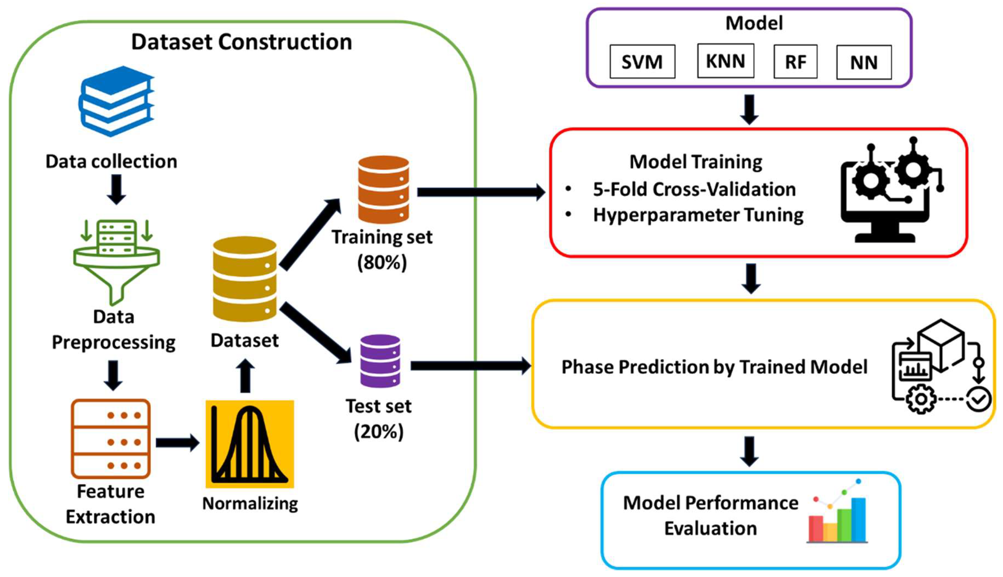
Figure 2.
Pair plot of features for phase categories. Abbreviations: Entropy of mixing (), Enthalpy of mixing (), Melting temperature (), Atomic size difference (), Valence electron concentration (), Parameter for predicting solid solution formation (), Electronegativity difference (), BCC (Body-Centered Cubic), FCC (Face-Centered Cubic), IM (Intermetallic).
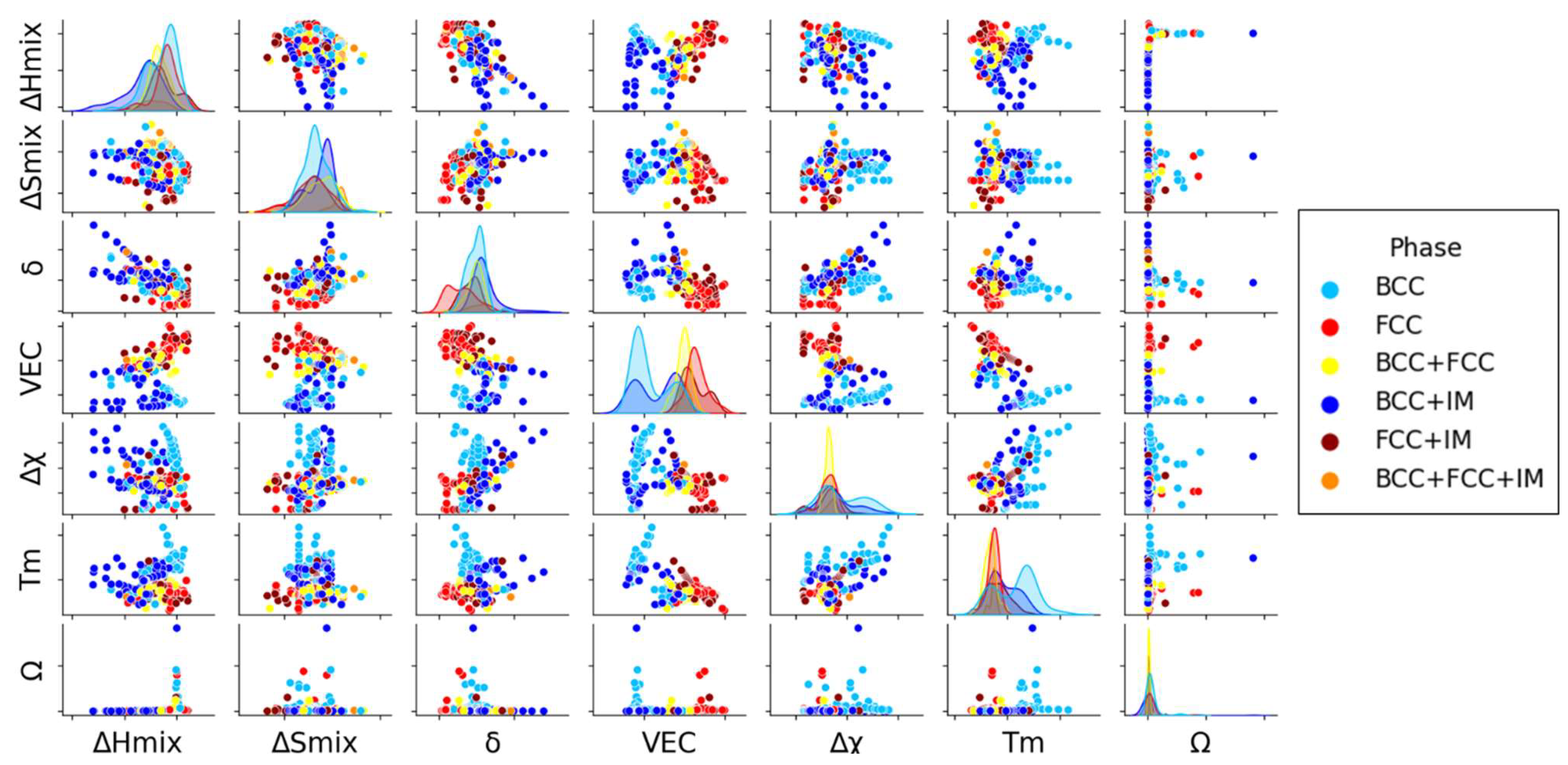
Figure 3.
Radar plot of features for phase categories of dataset. Abbreviations: Entropy of mixing (), Enthalpy of mixing (), Melting temperature (), Atomic size difference (), Valence electron concentration (), Parameter for predicting solid solution formation (), Electronegativity difference (), BCC (Body-Centered Cubic), FCC (Face-Centered Cubic), IM (Intermetallic).
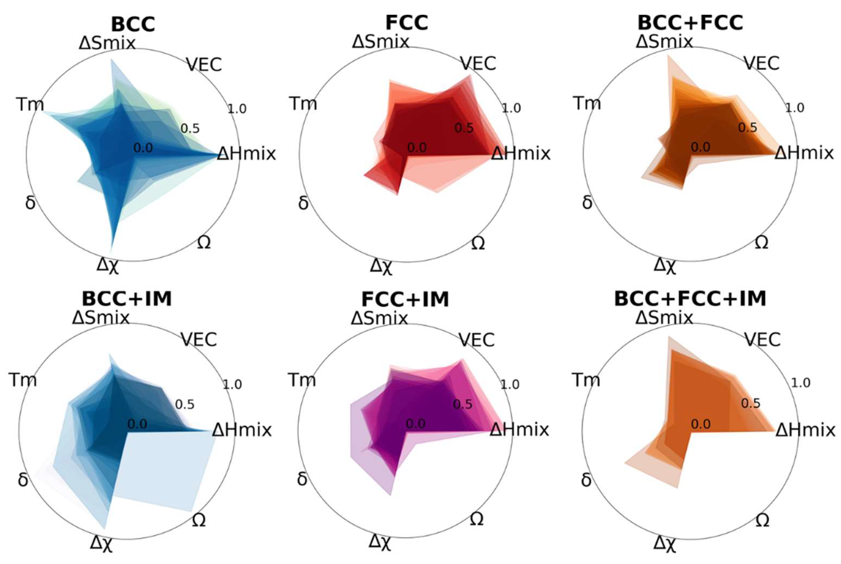
Figure 4.
Correlation heat map of feature relationships in dataset. Abbreviations: entropy of mixing (), enthalpy of mixing (), melting temperature (), atomic size difference (), valence electron concentration (), Parameter for predicting solid solution formation (), Electronegativity difference () .
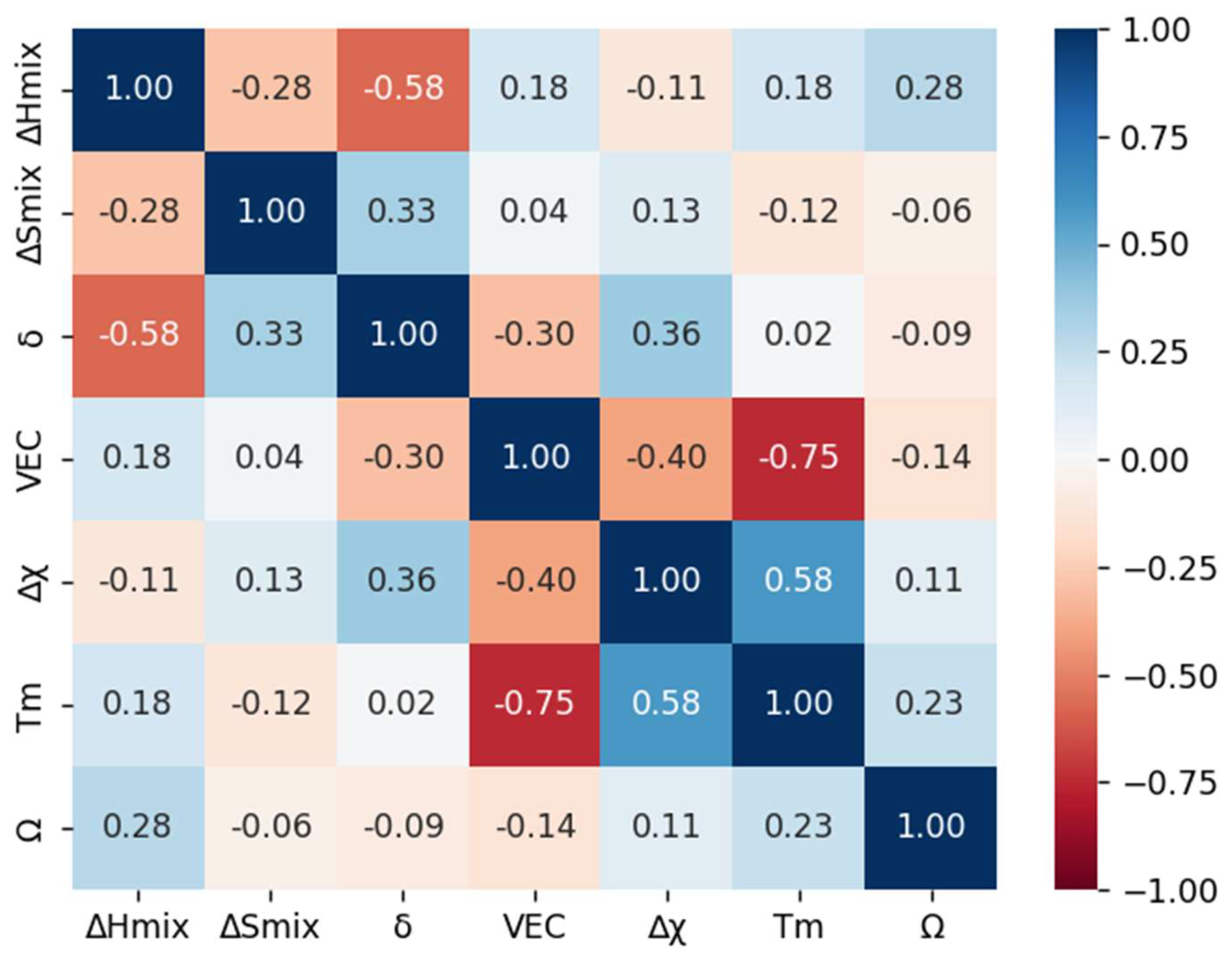
Figure 5.
The 3D scatter plot showing phase distribution to compare the effect of , and . Abbreviations: Entropy of mixing (), Enthalpy of mixing (), Melting temperature (), Atomic size difference (), Valence electron concentration (), Parameter for predicting solid solution formation (), Electronegativity difference (), BCC (Body-Centered Cubic), FCC (Face-Centered Cubic), IM (Intermetallic).
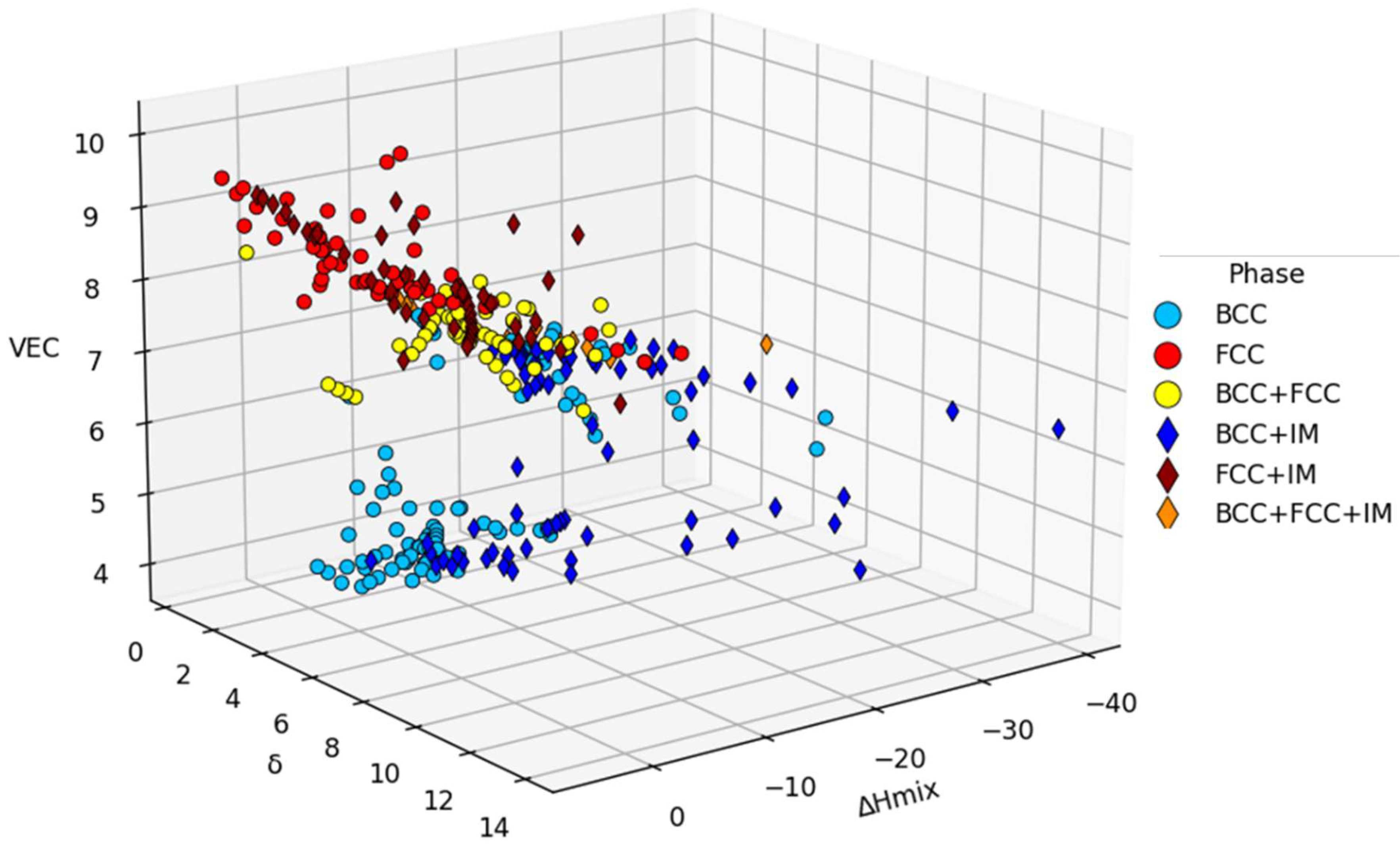
Figure 6.
Feature importance ranking for phase prediction in HEAs using the the RF classifier.
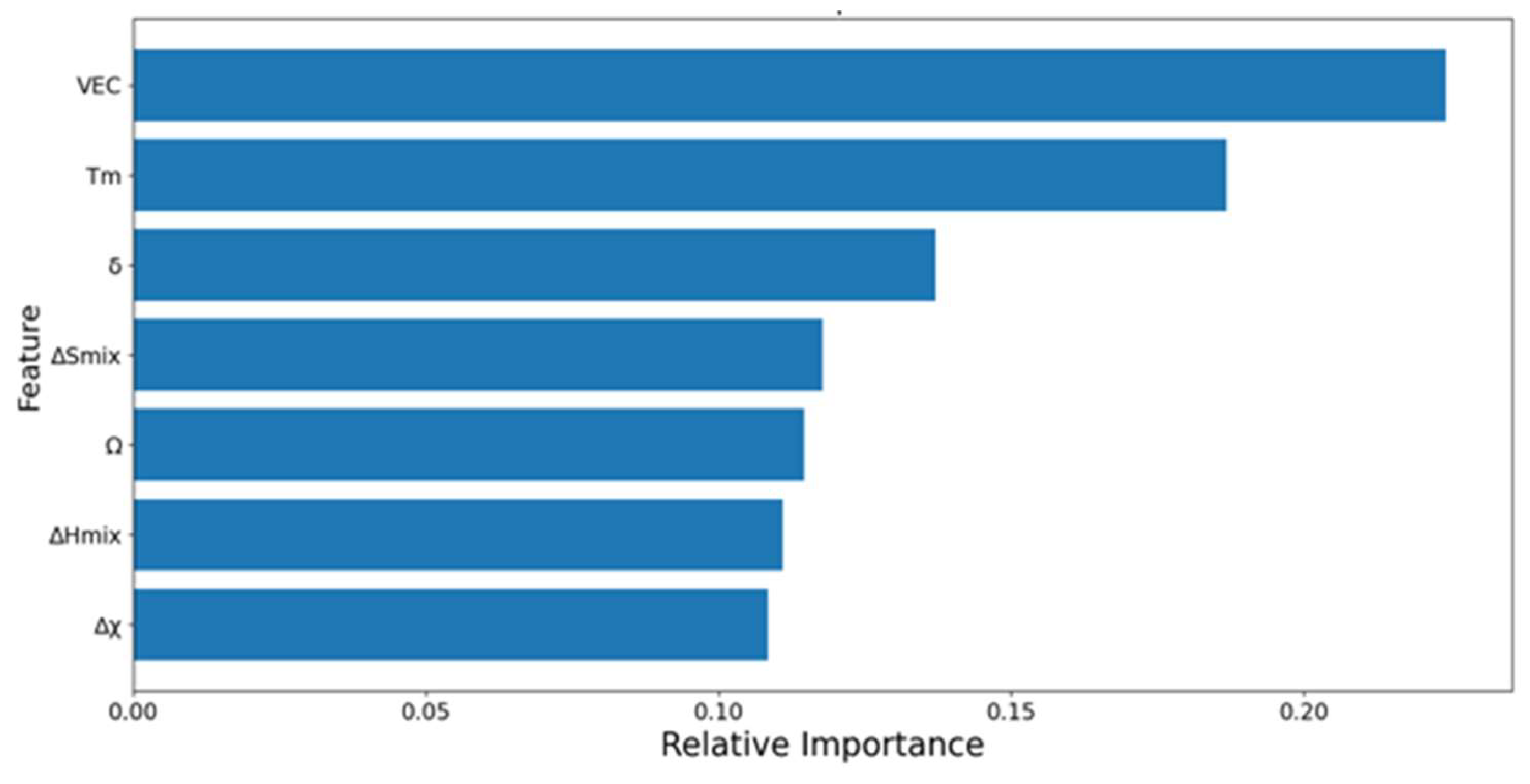
Figure 7.
Cross-validation and test accuracy of different models.
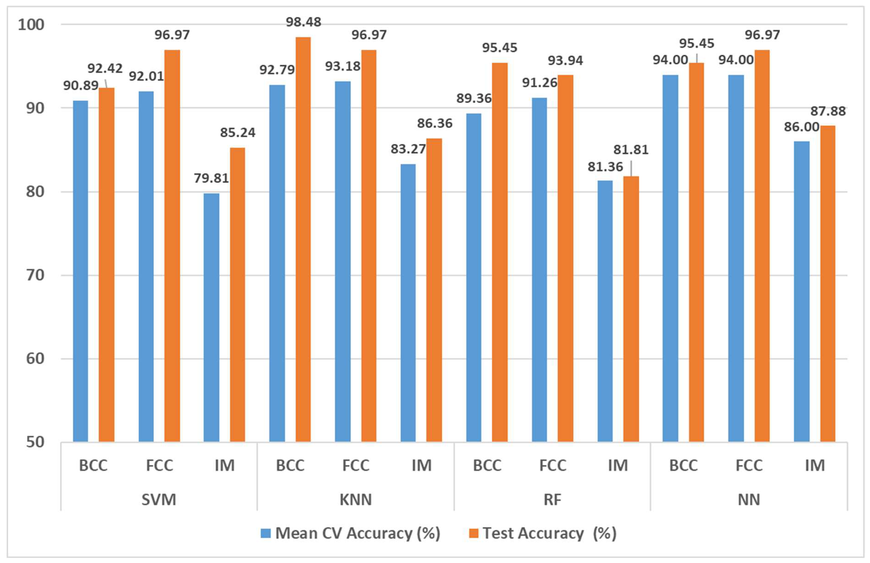
Figure 8.
ROC curve and PR curve for the NN.
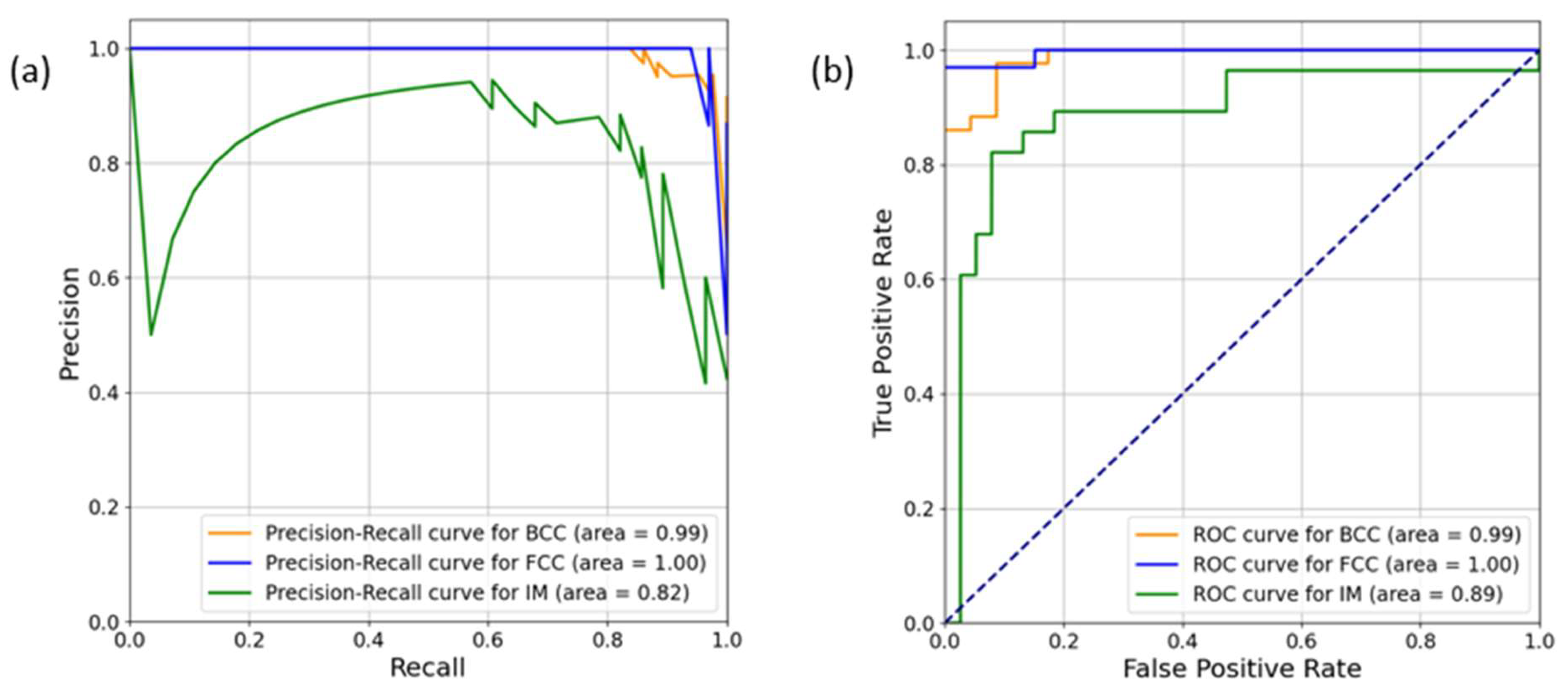
Figure 9.
Complex combination phase prediction accuracy of different models.
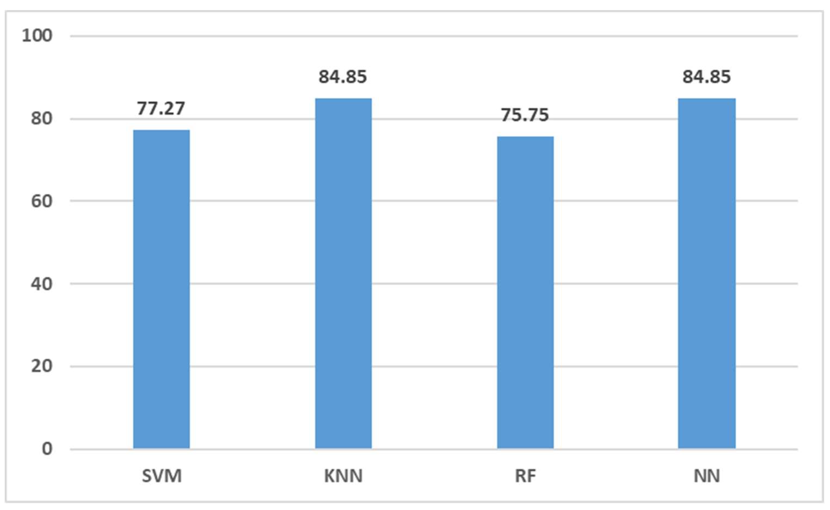

Table 1.
Example HEAs and their corresponding phases encoded as Boolean vectors.
| Alloys | Phase | BCC | FCC | IM |
|---|---|---|---|---|
| HfMoNbTaTiZr | BCC | 1 | 0 | 0 |
| CoCrFeMnNiV0.5 | FCC | 0 | 1 | 0 |
| CoCrFeMnNiV0.75 | FCC+IM | 0 | 1 | 1 |
| AlCrCuFeNi0.8 | BCC+FCC | 1 | 1 | 0 |
| AlCoCuFeNiZr | BCC+FCC+IM | 1 | 1 | 1 |
Footnote: In this equation, In these equations, represents the gas constant, and are atomic concentrations of the and components respectively, is an interaction parameter between the and elements, is the melting temperature of the component, is the atomic radius of the component, is the average atomic radius, is the valence electron concentration of the component, is the Pauling electronegativity of the component and is the average Pauling electronegativity.
Table 2.
Equations for feature extraction from chemical composition of alloys.
| Equation | Feature description | Reference |
|---|---|---|
| Mixing entropy | [66] | |
| Mixing enthalpy | [26] | |
| Melting temperature | [10] | |
| Parameter for predicting solid solution formation | [10] | |
| Atom size difference | [66] | |
| Valence electron concentration | [12] | |
| Electronegativity difference | [67] |
Table 3.
Hyperparameter selection and their ranges for the different models in this study.
| Model | Hyperparameter | Range of hyperparameter |
|---|---|---|
| SVM | C kernel gamma |
[1,10, 50, 100] rbf, poly, sigmoid [1, 10, 100] |
| KNN | N_neighbors weights P Algorithm |
range (1, 50) uniform, distance manhattan, Euclidean auto, ball_free, kd_tree, brute |
| RF | n_estimators max_depth min_samples_split min_samples_leaf |
[50, 100, 200] [None, 5, 10, 20] [2, 5, 10] [1, 2, 4] |
| NN | hidden_layer_sizes activation solver alpha |
[50, 100, 200] logistic, tanh, relu lbfgs, sgd, adam [0.0001, 0.001, 0.01] |
Table 4.
Cross-validation performance metrics of ML algorithms for each phase prediction in HEAs.
| Performance metric | SVM | KNN | RF | NN | ||||||||
|---|---|---|---|---|---|---|---|---|---|---|---|---|
| BCC | FCC | IM | BCC | FCC | IM | BCC | FCC | IM | BCC | FCC | IM | |
| Mean CV Accuracy (%) | 90.89 | 92.01 | 79.81 | 92.79 | 93.18 | 83.27 | 89.36 | 91.26 | 81.36 | 94.00 | 94.00 | 86.00 |
| Test Accuracy (%) | 92.42 | 96.97 | 85.24 | 98.48 | 96.97 | 86.36 | 95.45 | 93.94 | 81.81 | 95.45 | 96.97 | 87.88 |
| Precision (%) | 93.15 | 96.97 | 81.30 | 97.83 | 96.97 | 86.68 | 94.64 | 94.10 | 82.95 | 95.45 | 96.97 | 87.98 |
| Recall (%) | 90.14 | 96.97 | 82.15 | 98.48 | 96.97 | 85.34 | 95.50 | 93.94 | 79.98 | 94.49 | 96.97 | 87.12 |
| F1 score (%) | 91.38 | 96.97 | 82.15 | 98.48 | 96.97 | 85.81 | 95.04 | 93.93 | 81.39 | 94.94 | 96.97 | 87.46 |
Disclaimer/Publisher’s Note: The statements, opinions and data contained in all publications are solely those of the individual author(s) and contributor(s) and not of MDPI and/or the editor(s). MDPI and/or the editor(s) disclaim responsibility for any injury to people or property resulting from any ideas, methods, instructions or products referred to in the content. |
© 2025 by the authors. Licensee MDPI, Basel, Switzerland. This article is an open access article distributed under the terms and conditions of the Creative Commons Attribution (CC BY) license (http://creativecommons.org/licenses/by/4.0/).
Copyright: This open access article is published under a Creative Commons CC BY 4.0 license, which permit the free download, distribution, and reuse, provided that the author and preprint are cited in any reuse.


