
Submitted:
23 December 2025
Posted:
29 December 2025
You are already at the latest version
Abstract
A wide range of factors influences the dynamic and complex environment that is the commodity market. The most significant of these are external influences, such as political decisions and weather conditions, which cannot be directly controlled. Nevertheless, specific characteristics and price behaviors are exhibited by individual commodities, which manifest through seasonal patterns and characteristic fluctuations. This study aimed to analyses the day-ahead electricity market and identify the key factors influencing electricity price formation. Particular focus was given to the impact of meteorological variables and the interrelationships between the prices of other commodities, such as natural gas, coal and oil. A basic forecast of electricity prices in the day-ahead market was provided by a simple predictive model that was developed based on the findings. The results highlight the interconnectedness of energy markets and confirm that external factors play a crucial role in shaping electricity prices.
Keywords:
electricity market
; forecasting
; weather
; data analysis
; seq2seq
; LSTM
1. Introduction
Market uncertainty is currently having a significant impact on day-ahead electricity prices, which are shaped by a range of external factors, particularly global fluctuations in commodity markets. While the EU has made significant progress in increasing renewable energy capacity, a significant portion of electricity generation still relies on fossil fuels. This reliance is a key factor in determining prices, particularly during periods of increased volatility in international commodity market [1]. The liberalization and integration of electricity markets across Europe have further increased the complexity of price formation in the day-ahead market (DAM). As large-scale electricity storage remains economically challenging, DAM prices are highly sensitive to short-term supply and demand fluctuations. Therefore, understanding how exogenous variables influence DAM prices is crucial for market participants, system operators and policymakers [2].
Prices of energy commodities, including but not limited to crude oil, natural gas and coal, are amongst the most extensively studied external factors. These commodities are often used as marginal fuels in power generation, meaning that cost shocks can be transmitted directly into electricity markets by changes in their prices. [3], analyses 21 European markets, showing that natural gas price shocks propagate into electricity prices across various generation mix scenarios. In a similar context, [4] found that the transmission of gas price fluctuations to electricity prices has intensified across bidding zones, particularly following recent geopolitical disruptions. [5], in relation to this, identified significant mutual interaction between fossil fuel and electricity market.
In relation to this, significant bidirectional spillovers exist between the fossil fuel and electricity markets. The analysis emphasizes the strong impact of natural gas prices and weather-related factors, such as heating degree days. Alongside fossil fuel prices, meteorological variables also play a crucial part in determining day-ahead electricity prices. Weather conditions affect both electricity demand, through factors such as temperature and wind speed, and supply, particularly in systems with a growing share of variable renewable energy sources, such as wind and solar power [5].
It is key to understand these multiple drivers, as shown by the structural evolution of electricity generation in the EU Figure 1. As illustrated, the generation mix has been gradually transforming over recent years. A steady increase in the share of renewable energy sources has been seen, while a decline in generation from fossil fuels has been experienced. Nevertheless, fossil fuels continue to account for a significant proportion of total electricity production [6]. In contrast, nuclear power generation has remained stable, with only minor year-on-year fluctuations. This ongoing dependence on fossil fuels, despite the expansion of renewables, explains why commodity price shocks continue to significantly impact DAM prices, highlighting the importance of investigating their transmission mechanisms [7].
Although a substantial body of research has examined the influence of commodity prices and meteorological conditions on electricity markets, important questions remain regarding the relative and evolving importance of these factors in shaping DAM prices. While much of the existing literature has concentrated on forecasting accuracy or identifying long-term relationships, fewer studies have undertaken a comprehensive empirical analysis of how key external drivers such as fossil fuel prices, renewable generation, and demand conditions interact within specific market contexts [8].
Despite extensive evidence that renewable energy sources exert downward pressure on wholesale electricity prices across Europe [9] and globally [10], the joint dynamics between fossil fuel prices, variable renewable generation, and market design remain insufficiently understood. As renewable penetration increases and flexibility requirements grow, the sensitivity of DAM prices to traditional determinants—such as natural gas prices and system demand appears to be shifting.
Recent evidence from European markets indicates that gas prices and wind generation have become increasingly dominant determinants of DAM price formation, often surpassing conventional demand-related effects [11]. These developments highlight the need for renewed analytical focus on the structural drivers and transmission mechanisms of electricity prices, rather than on forecasting performance alone, to better understand how energy transitions reshape short-term market behavior.
2. Forecasting Electricity Price
Accurate electricity price forecasting enables market participants to optimize their trading strategies and minimize the risks associated with price volatility. For electricity producers, accurate forecasting is crucial for production planning and profit maximization, while distributors and large consumers use it to manage their purchasing portfolios and reduce costs [12]. In an environment with an increasing proportion of renewable energy sources and rising price volatility, the importance of reliable forecasting tools is growing, as the quality of forecasts directly affects the financial performance of energy companies [13]. Price predictions are relied on by system operators to ensure the balance between supply and demand is maintained and to identify potential network congestion [13]. With a growing share of intermittent renewable sources, price forecasting becomes more complex but essential for effective power system management, and its accuracy requires reliable tools for measuring and comparing different predictive models [14]. Forecast evaluation uses several metrics to measure the deviation between actual and predicted values. The choice of metric depends on the data type and the objective of the analysis [13]. Five commonly used error metrics are employed in this study to systematically evaluate forecast performance: mean absolute error (MAE), mean squared error (MSE), root mean squared error (RMSE) and mean absolute percentage error (MAPE), as well as the coefficient of determination (R²).
Where , , and are the sample size and the actual and predicted values, respectively [15].
2.1. Basic Forecasting Model
Forecasting electricity prices using prediction methods based on historical data is possible. [16] applied an artificial neural network (ANN) model in combination with the Markov Chain (MC) method to forecast electricity prices, with the aim of increasing prediction accuracy. For the study, the dataset was divided into two parts. The training set contained data from 2004 to 2018 and the test set covered the period from 2018 to 2020. The training set was used to implement the model and estimate its parameters. Results showed that the ANN model alone achieved a MAPE of 12.65% and MAE of $2.95/MWh. In contrast, the combined ANN-MC model demonstrated slight improvement, achieving MAPE and MAE values of 12.57% and $2.29/MWh, respectively. These results confirm that incorporating the Markov Chain method into the model increased the accuracy of electricity price predictions [16]. A variety of prediction models are used for short-term electricity price forecasting [17], [18] [19]. The methodologies that have been implemented for short-term forecasts in recent years can be categorized into regression models, such as Regression Splines Decomposition (RSD) and Smoothing Splines Decomposition (SSD) [20], neural network methods, specifically Long Short-Term Memory (LSTM) using Wavelet transform to prevent model fluctuations in prediction [17], and the extensive use of machine learning methods [18]. Table 2.1 provides an overview of the accuracy of these models [17], [18], [20]. Different models show varying degrees of accuracy in short-term electricity price forecasts, depending on the input data. The highest accuracy is achieved by the LSTM models when working with data divided into smaller time periods [17], but a significant advantage over alternative approaches is not shown by it when continuous data is used without this adjustment [18]. When working with continuous data, the Multi-Task Graph Neural Network (MTGNN) model tends to achieve higher prediction accuracy. Graph neural network (GNN) models perform better than Informer and ST-Norm models. This is due to the effective inclusion of spatial characteristics in the prediction. Examples of GNN models include Multi-Graph Adversarial Attention Learning (MGAAL) and Adaptive Spatial-Temporal Graph Convolutional Network (ASTGCN). The MGAAL model achieves the best performance on most evaluation metrics across different prediction horizons [18]. Significant regional differences in prediction accuracy have been identified, with prices in areas with a higher share of renewable energy sources showing greater fluctuations and being more difficult to predict. In contradistinction to artificial neural network-based approaches, decomposition models such as Residual Seasonal Decomposition (RSD) focus on the decomposition of time series data into long-term trend, seasonal and residual components [20]. This separation enables more accurate modelling of hidden patterns, particularly in datasets with strong seasonality or irregular trends. When configured correctly, the RSD model can significantly improve the accuracy of short-term electricity price prediction and other continuous data forecasting. According to study [20], specific RSD model combinations achieve the lowest mean prediction errors, with performance varying slightly by season achieving the highest accuracy in spring and slightly higher, yet still acceptable, errors in summer.
2.2. Forecasting with Multiple Input Data
Hyperparameter-based models are used to predict electricity prices over longer time horizons. These models also use other data affecting electricity prices to make predictions [21]. The use of electricity prices and consumption levels was the approach taken in these cases. Predicting prices based on multiple data points is a relatively complex process that requires thorough data analysis. [21] used Fourier series to analyses the data, enabling him to effectively approximate the electricity price profile. We define the approximation of the non-new profile as follows:
where ft is the approximate price of electricity at time t, consisting of the main frequency components of the Fourier series, a0 represents the mean value of pt and an, bn are the Fourier coefficients that define the shape of the periodic functions at frequency n, with N representing the length of the original time series.
While this approximate price captures the basic development of the electricity price, it cannot describe hourly fluctuations or periods of extreme prices that exceed the basic patterns of the price profile. These fluctuations are described by the residual term Rt, which consists of all frequency dependencies. Three predictive models were employed by [21] to forecast electricity prices Linear Regression, Gaussian Process Regression (GPR), and ANN. The GPR model achieved the best overall performance among these, with the MAPE of approximately 13.5% for multi-output configurations and 13.2% for single-output configurations. By comparison, the linear regression model produced higher errors of 18.9% and 19.2%, while the ANN model produced intermediate accuracy with errors of 14.3% and 15.2% respectively. These results suggest that GPR offers the most reliable and consistent forecasts for predicting electricity prices over extended time horizons [21].
[22] proposed a multivariable bi-forecasting system for predicting electricity prices that integrates point and interval forecasting in order to overcome the limitations of single-variable and single-output models. This begins with data pre-processing using Improved Complete Ensemble Empirical Mode Decomposition with Adaptive Noise (ICEEMDAN) to enhance the quality of electricity price and load data by eliminating noise. A rolling forecasting framework with multi-input and multi-output structures is then constructed to combine electricity prices and power demand, improving prediction stability and accuracy. A hybrid predictive model employing linear operators is then established, with its parameters optimized using the Multi-Objective Golden Eagle Optimizer (MOGEO) algorithm. Experimental results using New South Wales datasets demonstrated superior performance in terms of both point and interval forecasting accuracy, confirming the robustness and effectiveness of the method [22].
Forecasting electricity prices is a complex process involving varying models, which differ depending on the number of factors taken into account and the time horizon of the forecast. The majority of models concentrate on a restricted number of input parameters, with certain predictions being based on a few primary factors, such as fuel prices and electricity consumption requirements [23]. High accuracy in short-term forecasts is achieved by these models, with minute-by-minute or hour-by-hour forecasts being focused on. They utilize historical data and incorporate operational data from networks in their analysis, which can unveil patterns in electricity consumption and generation over time [24]. But when they try to predict what prices will be in the long term, these models often produce results that differ significantly from the actual prices. This suggests a lack of capability in the prediction of long-term price changes. Other models take a wider range of factors into account, such as fuel prices, political decisions, power plant outages, renewable energy production and meteorological conditions that directly affect renewable energy production [25]. These models provide more accurate and comprehensive forecasts. These models are primarily used for short-term predictions, enabling minute-by-minute or hour-by-hour price fluctuations to be predicted, which is crucial for market participants who must adapt to rapidly changing conditions. For longer time periods, the focus is on macroeconomic factors such as global energy demand, political factors and technological advances in renewable energy in order to assess price fluctuations and risks associated with future market developments [26]. Models such as AleaSoft and Enerdata apply advanced machine learning techniques and econometric approaches, integrating factors such as fuel prices, market sentiment, political changes, power plant outages and other relevant information [27], [28]. These factors have a strong short-term impact on electricity prices. They enhance forecast accuracy and support risk identification in both real-time and long-term markets. However, such models are usually available only to commercial subscribers, and their data are not publicly accessible.
2.3. Electricity Price Prediction Using Optimization Methods
Electricity price prediction models are increasingly being optimized, with the aim of improving the accuracy of predictions and reducing the impact of price fluctuations on consumers. The accuracy of prediction models is significantly improved by these methods, which adjust their parameters to minimize errors and maximize output accuracy [29]. The optimization process is carried out at several levels, with a key role being played by hyperparameter tuning in influencing the model’s effectiveness. Common approaches to identifying optimal parameter combinations include grid random search (RS) [30]. However, for models with a large number of parameters, more advanced optimization algorithms such as the Particle Swarm Optimization (PSO) and Genetic Algorithm (GA) need to be applied [30], [31]. As part of the optimization process, datasets from the English and German electricity markets were used to train a Convolutional Neural Network (CNN) with a Bidirectional-LSTM architecture, for which GA and Random Search (RS) methods were implemented. The application of these methods resulted in a substantial enhancement in prediction accuracy, with the PSO method attaining the desired deviation. Subsequent research [30], focused on improving the accuracy of LSTM, Recurrent neural network (RNN) and Backpropagation (BP) models by integrating decomposition techniques, such as Variation Mode Decomposition (VMD), with an Attention mechanism (ATT) and Grey Wolf Optimizer (GWO). The best results were achieved by models combining all three techniques, as was confirmed by testing various combinations of these approaches [31]. As shown in Table 2.2, the VMD-GWO-ATT-LSTM model achieved the lowest errors (RMSE = 1.78 €/MWh and MAE = €1.45/MWh), confirming that integrating optimization and decomposition methods can significantly improve the ability of models to accurately predict short-term movements in electricity prices [30], [31]. The performance metrics of the optimized models are summarized in Table 2.2 [30], [31]. The accuracy of short-term electricity price forecasts has been shown to be improved by combining advanced optimization models with hybrid architectures [29]. In comparison to earlier models that relied exclusively on rudimentary methods without resorting to optimization techniques [17], [18], [20], the implementation of sophisticated algorithms such as particle swarm optimization, genetic algorithms, grey wolf optimizers and Bayesian optimization algorithms led to a substantial reduction in prediction errors across a range of model architectures. The best results were achieved by the integration of these optimization methods with decomposition techniques such as variational mode decomposition and the attention mechanism [31].

Table 2.2.
Prediction accuracy based on performance metrics with optimalizations.
| Model | - | RMSE (€/MWh) | MSE (€/MWh) | MAE (€/MWh) |
| CNN-BiLSTM-AR | Data1 | 3.80 | 14.45 | 2.33 |
| RS-CNN-BILSTM-AR | Data1 | 3.62 | 13.09 | 2.16 |
| GA-CNN-BiLSTM-AR | Data1 | 3.71 | 13.76 | 2.21 |
| PSO-CNN-BiLSTM-AR | Data1 | 3.46 | 12.00 | 2.00 |
| Model | - | RMSE (€/MWh) | MSE (€/MWh) | MAE (€/MWh) |
| CNN-BiLSTM-AR | Data2 | 4.87 | 23.76 | 3.33 |
| RS-CNN-BILSTM-AR | Data2 | 4.64 | 21.62 | 3.07 |
| GA-CNN-BiLSTM-AR | Data2 | 4.46 | 19.92 | 2.87 |
| PSO-CNN-BiLSTM-AR | Data2 | 4.05 | 16.47 | 2.55 |
| Model | - | RMSE (€/MWh) | Mape (€/MWh) | MAE (€/MWh) |
| LSTM | Data3 | 2.88 | 1.99 | 2.29 |
| RNN | Data3 | 2.96 | 2.04 | 2.30 |
| BP | Data3 | 3.04 | 2.13 | 2.51 |
| ATT-LSTM | Data3 | 2.79 | 1.92 | 2.22 |
| ATT-RNN | Data3 | 2.93 | 2.03 | 2.37 |
| ATT-BP | Data3 | 2.95 | 2.06 | 2.39 |
| GWO-ATT-LSTM | Data3 | 2.74 | 1.72 | 2.00 |
| GWO-ATT-RNN | Data3 | 2.88 | 1.89 | 2.21 |
| GWO-ATT-BP | Data3 | 2.92 | 1.83 | 2.12 |
| VMD-LSTM | Data3 | 2.13 | 1.63 | 1.87 |
| VMD-RNN | Data3 | 2.98 | 1.45 | 2.05 |
| VMD-BP | Data3 | 2.35 | 1.79 | 2.04 |
| VMD-ATT-LSTM | Data3 | 1.96 | 1.43 | 1.66 |
| VMD-ATTT-RNN | Data3 | 2.17 | 1.59 | 1.85 |
| VMD-ATT-BP | Data3 | 2.18 | 1.60 | 1.87 |
| VMD-GWO-ATT-LSTM | Data3 | 1.78 | 1.24 | 1.45 |
| VMD-GWO-ATT-RNN | Data3 | 1.87 | 1.33 | 1.54 |
| CMD-GWO-ATT-BP | Data3 | 1.97 | 1.37 | 1.59 |
3. Data Description and Methodological Framework
To understand the electricity market, it is necessary to analyses the DAM in detail, because it represents a key segment of short-term electricity trading and interacts closely with other energy commodities. The data used for this analysis was obtained from the public-available OKTE [32] source and relates to the Slovak electricity market. To enable automated historical data retrieval within the required time frame, an API was implemented [33]. Data processing and analysis were carried out in the Python programming language using the JSON library to load and process files. Data covering the period from January 1st 2020 to June 30th 2025 was obtained from the day-ahead market database, with all data recorded at hourly intervals. Fast Fourier Transform (FFT) and Autocorrelation coefficient were then implemented to identify periodic patterns and dominant frequency components in the time series.
As shown in Figure 2 and Figure 3, two methodologies were used to identify periodic patterns in electricity prices, showing three main cycles: daily, weekly and semi-daily. Analyzing a smaller subset of the data in Figure 2 reveals that the filtered data more closely follows real values than when a longer period is analyzed in Figure 3. The noise distribution graph shows that the residual component is approximately normally distributed around zero. This suggests that most deviations from the filtered signal are random, and that the filtering process effectively captures the dominant periodic patterns in DAM prices. Between 2020 and 2023, the world faced a number of major crises, which caused significant disruption to commodity markets and typical price dynamics. This led to a more volatile and sudden fluctuations in prices. These outcomes are consistent with recent studies by [34] and [35] which emphasize the significant sensitivity of commodity prices to external and uncontrollable factors, such as geopolitical tensions and global changes. [34] demonstrated that the volatility and spillover effects across fossil energy, electricity, and carbon markets were substantially increased by the effects of the pandemic and the Russia–Ukraine conflict, while [35] highlighted synchronized changes in oil, coal, and natural gas markets driven by uncertainty, investor sentiment, and structural market.
Even within the shorter timeframe of 2023–2025, daily, weekly, seasonal and sub-seasonal cycles are evident, suggesting that predictive models for DAM prices should be able to capture long-term cyclical behavior using limited historical data. However, extending the analysis to the period from 2020 to 2025 provides a clearer identification of seasonal and semi-annual patterns influenced by broader market and macroeconomic factors.
Table 3.1.
Comparison of dominant periodicities for different data lengths.
| 2023 - 2025 | 2020 - 2025 | |||||
| Rank | Period (d) | Extent (EUR/MWh) | Type | Period (d) | Extent (EUR/MWh) | Type |
| 1 | 1.00 | 49.00 | Daily | 7.01 | 31.86 | Weekly |
| 2 | 0.50 | 39.90 | Half-daily | 1.00 | 29.92 | Daily |
| 3 | 7.01 | 17.74 | Weekly | 0.50 | 25.15 | Half-daily |
| 4 | 82.82 | 8.79 | Seasonal | 143.36 | 15.44 | Long-seasonal |
| 5 | 3.50 | 8.65 | Sub-weekly | 91.23 | 13.56 | Seasonal |
| 6 | 75.92 | 7.62 | Seasonal | 133.8 | 12.77 | Long-seasonal |
| 7 | 53.59 | 7.43 | Bi-monthly | 118.06 | 11.91 | Long-seasonal |
| 8 | 33.74 | 7.23 | Monthly | 154.39 | 11.89 | Half-Yearly |
| 9 | 130.15 | 7.10 | Long-seasonal | 167.25 | 11.78 | Half-Yearly |
| 10 | 91.10 | 7.03 | Seasonal | 52.82 | 11.53 | Bi-monthly |
In today’s highly interconnected global economy, commodity markets are increasingly interdependent, with price movements in one market often influencing others. Numerous studies have demonstrated significant interlinkages among commodities — for instance, electricity prices are closely tied to the dynamics of emission allowance markets and fossil fuel prices. For example, Energy commodities spillover analysis for assessing the functioning of the European Union Emissions Trading System trade network of allowances shows that energy commodity shocks (brent, coal, gas) act as transmission channels into the European Union Emissions Trading System network of allowances, making the carbon-market network a net receiver of spillovers from energy markets [36].Similarly, the study Alarming contagion effects the dangerous ripple effect of extreme price spillovers across crude oil, carbon emission allowance and agriculture futures markets finds that under extreme market conditions, the interdependence among crude oil, carbon emission allowances, and other commodity futures can surge dramatically, reducing diversification benefits and increasing systemic risk [37]. Another investigation, A Study Based on Positive and Negative Price Volatility, identifies that feedback loops exist between energy and carbon markets, where volatility shocks in fossil fuel markets propagate into carbon pricing, demonstrating a contagion pathway across commodity systems [38]. Moreover, [39] found dynamic bidirectional volatility spillovers between carbon and energy markets, confirming the presence of persistent co-movements across energy commodities. These findings consistently indicate that fossil fuels, electricity, and emission allowances form a tightly connected network in which shocks in one market can rapidly transmit to others, influencing both pricing behaviour and market stability.
Historical commodity price data were obtained from Yahoo Finance using the yfinance Python library [40], while electricity price data were sourced from the OKTE day-ahead market platform [33]. Our comparative analysis focuses on the year 2024, for which complete datasets across all examined commodities are available. Before computing correlation coefficients, it is essential to ensure that all datasets have consistent lengths and comparable temporal characteristics. Commodities such as crude oil and electricity [33] provide daily trading values, whereas other commodities exhibit different temporal resolutions. To address this, we adopt an approach that considers relative price changes over time, enabling meaningful comparison across markets. Specifically, daily price variations are analyzed to capture year-long dynamics. Natural gas trading occurs during specific hours (8:00–22:00), coal prices are updated once per day, emission allowances are traded continuously within a 24-hour window, and uranium prices, similar to coal, are revised once daily.
Figure 4 shows a positive correlation between electricity prices and three selected commodities: natural gas, emission allowances and coal. The strongest positive correlation (r = 0.59) was observed between electricity and natural gas, suggesting that gas plays a key role in electricity pricing, particularly given the significant proportion of electricity produced by gas-fired power plants. The moderately positive correlations with emission allowances (r = 0.28) and coal (r = 0.14) imply that these commodities may also impact electricity prices to some extent, primarily through emission costs and fuel substitution. On the other hand, the negative correlations seen among electricity and Brent crude oil (r = −0.48) and Uranium (r = −0.47) imply that these markets might be driven by different dynamics, influenced by factors not directly connected to the electricity market, such as macroeconomic cycles, geopolitical events or specific nuclear sector developments. As well as the previously mentioned correlations between electricity prices and specific commodities, additional interconnections can be seen between the commodities themselves. For example, gas shows a positive correlation with emission allowances and a negative correlation with coal, while it correlates negatively with Brent crude oil and uranium. Emission allowances are positively linked to coal, but have weaker or negative relationships with other fuels. There is a slightly positive correlation between Brent crude oil and Uranium.
The aim of the second part of the data analysis is to determine the potential impact of weather factors on electricity prices. As in the previous case, this step involves comparing parameters received from the OKTE platform with historical meteorological data obtained from the Historical Weather API [32], [41]. Since only variables for 2024 were included in the previous part of the analysis, data from the same period is used in this case as well. Five meteorological variables were received from the API: air temperature, wind speed, precipitation, humidity and cloud cover [41]. Contrary to the previous database, where it was required to summaries the data into daily values, the data in this case is provided in hourly intervals. For analysis purposes, all variables were normalized into relative units, since individual meteorological variables differ in their physical scales. This process of standardization enables the comparison of these values and prevents any distortion of the results of the correlation analysis. When looking at how weather affects things, it is important to remember that, unlike with other products, the weather can have a positive or negative correlation on the price of electricity.
The average correlation between weather variables and electricity prices depending on the hour of the day is shown in Figure 5. This has been calculated using a 24-hour rolling window. As can be seen from the graph, the correlation varies significantly throughout the day. During the day, there is a notable negative relationship between temperature and time, with a peak of around -0.5 at midday. However, this shifts to
positive correlation at night. The opposite pattern is exhibited by relative humidity, which has a positive correlation during the day, peaking at around 0.5, and a negative correlation at night. A slight negative correlation is shown by wind speed, which remains relatively stable throughout the day. The correlation values of cloud cover and precipitation are smaller and more variable. Renewable energy sources, especially solar and wind, are likely having an impact on electricity prices, which is probably the reason for these distinct daily patterns in correlation. The observed relationships are also significantly influenced by daily consumption profiles and seasonal factors. Figure 5 shows average values only and cannot capture the full range of variability in correlations that occur at different times and under different conditions.
Figure 6 was created to analyses the distribution of correlation coefficients between electricity prices and individual weather variables in detail. The histograms show how frequently different correlation values occurred during the analyzed period. These reveal that all weather variables exhibit a significantly wider range of correlation values, ranging from strongly negative to strongly positive, than the average values shown in Figure 5 suggest. Temperature tends to be negatively correlated with electricity prices, with a significant shift in the distribution towards negative values. This suggests that rising temperatures are linked to falling prices. A distribution that is shifted towards higher values is often associated with increased relative humidity. Wind speed, cloud cover and precipitation exhibit a relatively symmetrical distribution of correlations around zero, but with a wide range of values. Figure 6 cumulative histogram reveals considerable overlap in the correlation values of the individual parameters across the entire spectrum from -1 to +1, despite their different distribution characteristics. This indicates a complex interaction between weather variables and electricity prices that is not apparent from average values alone.
When considering the impact of weather on various factors, it is important to note that, unlike other products, weather can positively or negatively affect the price of electricity. This concept is reflected in recent research. In the study [42] have demonstrated that weather conditions and climate change significantly influence wholesale electricity prices, with both extremely low and high temperatures leading to price increases due to increased demand for heating and cooling. Similarly, [43] emphasize that a simultaneous hedging strategy for price and volume risks in electricity businesses using energy and weather derivatives, noting that variations in temperature and wind speed represent key risk factors in electricity markets, affecting not only consumption but also price volatility. Furthermore, [44] presents evidence suggesting that weather-related variations in electricity demand, particularly those associated with heating and cooling requirements, vary considerably between high-income and middle-income countries. The analysis indicates that middle-income economies, characterized by rapid electrification and growing cooling needs, exhibit greater demand elasticity in response to temperature changes, whereas electricity consumption in high-income OECD countries remains more sensitive to heating requirements.
4. Application of the Proposed LSTM-Seq2Seq Model to Day-Ahead Market Prices
The development and evaluation of electricity price prediction models in this study are based on the analysis of data obtained from the day-ahead market, which were discussed in detail in the previous chapters. In 1997 [45] developed the LSTM model to solve issues faced in RNN learning. Problems such as an increase or loss of gradient value during learning are often encountered in traditional learning methods, such as backpropagation through time (BTT) and recurrent learning (RL). These inaccuracies caused the model to be unstable and learning to be inefficient, especially when working with longer time dependencies. The distinctive architecture of LSTM models is pivotal to their capacity to solve these problems, as it facilitates consistent learning over very long periods. This method guarantees that data is kept for the duration of the learning process, allowing models to successfully learn even with extended time dependencies while maintaining the capacity to process short-term data [46]. Due to these properties, LSTM models have become extremely advantageous in domains such as speech recognition, image and time series processing, all of which require long-term memory.
Based on our previously developed LSTM model with a sequence-to-sequence (seq2seq) architecture, this study applies the corresponding modelling framework to a new forecasting domain. In our earlier work [47], we used real data from photovoltaic systems and smart meters to train the model to predict household electricity consumption and production. Seq2seq architecture combines an encoder–decoder structure to enable the model to capture nonlinear and long-term temporal dependencies within time-series data effectively. In the present research, we have adapted this framework to forecast short-term electricity market prices. The model’s underlying architecture, training methodology and parameter configuration remain similar to those described in [47], ensuring comparability of results while extending the model’s applicability to a different dataset and forecasting objective. Further technical details are provided in Appendix B.
4.1. Processing of Data from the Day-Head Market
The initial stage of the forecasting procedure involved comprehensive planning and management of the data. The dataset was examined and cleaned, revealing that there were no gaps or missing values in the time series. This allowed for their direct application in modelling and prediction. Figure 7 shows all the data used to create the prediction models and displays average daily prices for the period from 2020 to 30 June 2025. Based on the FFT and ACF results, two approaches were defined for training the models, using different time ranges for the training and testing data.
- The first approach involved using data from the entire 2020–2025 period to train the model, with testing performed on the 2025 data remaining.
- The second approach employed the same division principle; however, the model was trained using data from 2023–2025, and the test set comprised the remaining 2025 data.
For both datasets, the data were partitioned into training and testing subsets using an 80:20 ratio, ensuring that 80% of the data were used for model training and the remaining 20% for testing. As shown in Figure 8, in the first instance (blue histogram), all the data available from the 2020–2025 period were included in the learning and testing process, while in the second instance (red histogram), solely data from the 2023–30th June 2025 period was utilized. Fourier analysis confirmed that both sets exhibited the same range of dominant frequencies, indicating that shortening the time range did not negatively impact the quality of the results. At the same time, the smaller data range enabled faster model training with only a slight loss of accuracy, as demonstrated by the previous analysis results.
In Table 4.1, the different configurations of the forecasting model are presented, illustrating how variations in sequence length, forecast horizon, and the number of training epochs influence the resulting performance metrics. All experiments were conducted on a GF76 11UC laptop, equipped with an 11th Gen Intel® Core™ i7-11800H processor operating at 2.30 GHz, 32 GB of RAM with a speed of 3200 MT/s, and an NVIDIA GeForce RTX 3050 Laptop GPU. These hardware specifications define the computational environment in which the model was trained and therefore provide important context for interpreting the training times and overall efficiency of the individual configurations.
In the context of 24-hour ahead forecasting, the utility of employing the complete 2020-2025 dataset remains ambiguous. Though a bigger data set provides more information about historical price movements, incorporating it into the model requires substantially more computing power and longer training times. Using a smaller subset of data, such as from 2023–2025, enables faster training. However, when considering the potential extension of the model to incorporate multiple input variables in the future, it is unclear whether prediction accuracy would be maintained, improved or reduced with a smaller data window. Therefore, careful selection of the input data and its historical range is crucial for balancing the trade-off between computational efficiency and achievable accuracy in short-term forecasts.
5. Conclusion
This study provides a thorough review of the factors that influence prices in the day-ahead market. It combines an analysis of commodity market dynamics and meteorological conditions with data-driven forecasting methodologies. The analysis confirms that electricity prices are highly sensitive to external changes, particularly to the prices of natural gas and emission allowances, and to extreme weather conditions. Despite the increasing use of renewable energy sources, fossil fuels still determine the marginal price for many hours of the year, explaining the strong positive correlation between DAM prices and natural gas markets.
The results also suggest that improving predictive accuracy could be achieved by extending the model to a multivariate framework incorporating factors such as commodity prices, meteorological variables and renewable generation profiles. However, this would require careful balancing of model complexity, data availability, and training efficiency. The complex effects observed in the studies of commodities and weather demonstrate the advantages of using multiple types of deep neural architecture, particularly those that employ attention mechanisms.
In terms of the approach used, the investigation reveals that state-of-the-art machine learning models, in particular the LSTM Seq2Seq framework, possess significant potential for brief price forecasting. Moreover, the implementation of FFT and autocorrelation analysis was instrumental not only in identifying prevailing daily, weekly, and seasonal cycles, but also in formulating a discrete cyclical reconstruction of price dynamics. This breakdown made it easier to understand the underlying pattern of prices on the DAM, and it provided a way to compare LSTM predictions. Comparing the training datasets revealed important trade-offs: using the full dataset from 2020 to 2025 improved the accuracy of medium-term predictions (12–24 hours), while training on the shorter dataset from 2023 to 2025 provided better results for very short-term predictions (one hour ahead) and significantly reduced computational costs. The results suggest a dependence of the optimal historical window range on the forecast horizon and the volatility regime of the relevant market.
The findings also indicate that extending the model to a multivariate framework including commodity prices, weather variables, or renewable generation profiles could further enhance predictive accuracy. However, such an expansion may require careful balancing between model complexity, data availability, and training efficiency. The strong spillover effects observed in the commodity analysis and the nonlinear meteorological influences underscore the potential benefits of multi input deep learning architectures, particularly those integrating attention mechanisms or graph-based structures.
Overall, this study contributes to a deeper understanding of the structural drivers shaping DAM price dynamics and evaluates the practical feasibility of accessible forecasting tools built on publicly available data. The results demonstrate that reliable short-term forecasting is achievable using open datasets and computationally manageable models, providing added value for market participants. In addition, this approach provides an accessible alternative for smaller consumers and market participants who wish to operate actively in the short-term electricity market but prefer not to invest in commercial forecasting services or costly analytical tools.
Despite its contributions, the study is subject to several limitations. The forecasting model relies exclusively on historical price data, meaning that causal relationships with exogenous variables—such as fuel prices, emissions, renewable availability, demand levels, and policy changes—are not explicitly captured. In addition, the analysis is confined to the Slovak bidding zone, which limits the ability to account for cross-border flow constraints, market-coupling effects, and regional interactions that play an increasing role in European electricity price formation.
Future research should therefore focus on expanding the forecasting framework to incorporate multiple input variables, including natural gas prices, carbon emission allowances, renewable generation forecasts, weather conditions, and system load indicators. Integrating such parameters into a multivariate deep-learning architecture is expected to improve both accuracy and robustness, especially during high-volatility episodes. Extending the analysis to include market-coupling data, cross-border flow patterns, and neighboring bidding zone prices would also offer a more complete view of the structural determinants of DAM price formation.
Author Contributions
Martin Matejko: Conceptualization, Methodology, Software, Data curation, Formal analysis, Investigation, Visualization, Writing – original draft, Writing – review & editing. Peter Braciník: Conceptualization, Supervision, Resources, Writing – review and editing.
Funding
This research received no external funding.
Data Availability Statement
The original contributions presented in this study are included in the article trough API: https://github.com/ranaroussi/yfinance, https://www.okte.sk/en/api-documentation/short-term-market/dam-results/, and https://github.com/open-meteo/open-meteo.
Conflicts of Interest
Conflicts of Interest: The authors declare no conflict of interest.
Appendix A. Model
A.1. Model Architecture
The forecasting model employs a sequence-to-sequence (Seq2Seq) architecture based on Long Short-Term Memory (LSTM) networks, implemented using Keras/TensorFlow. The architecture consists of an encoder-decoder structure designed to capture temporal dependencies in electricity price time series data.
Table A1.
LSTM-Seq2Seq model architecture summary.
| Component | Layer Type | Unit/Config | Activation | Parameters |
| Encoder | LSTM | 128 unit | tanh | 66 560 |
| Dropout | Rate=0.2 | - | 0 | |
| Repeat vector | 84 repetitions | - | 0 | |
| Decoder | LSTM | 64 unit | tanh | 49 408 |
| Dropout | Rate=0.2 | - |
A.2. Hyperparameters
The model hyperparameters were configured based on preliminary experimentation and computational constraints. All hyperparameters are listed in Table A.2.
Table A2.
Model hyperparameters.
| Parameters | Value |
| Optimizer | Adam |
| Learning rate | Default (0.001) |
| Loss function | MSE |
| Batch size | 64 |
| Maximum Epochs | 100 |
| Early stopping | 10 epochs |
| Early stopping monitor | Validation loss |
| Restore best weights | True |
| Activation function (hidden layer) | Tanh |
| Activation function (output layer) | Linear |
| Dropout rate | 0.2 |
B.3. Data Preprocessing
B.3.1. Normalization
All price data were normalized using Min-Max scaling to the range [0, 1] [47]:
P is the current value, Pₘᵢₙ is the minimum, Pₘₐₓ is the maximum, and Pₙₒᵣₘ is the normalized value between 0 and 1.
B.3.2. Sequence Generation
Time series data were transformed into a supervised learning format using a sliding window approach. Let be the time series, the sequence length, and the forecast length. The input sequences and target sequences are defined as:
for .
References
- Hille, E. Europe’s energy crisis: Are geopolitical risks in source countries of fossil fuels accelerating the transition to renewable energy? Energy Economics 2023, vol. 127, 107061. [Google Scholar] [CrossRef]
- Liebensteiner, M.; Ocker, F.; Abuzayed, A. High electricity price despite expansion in renewables: How market trends shape Germany’s power market in the coming years. In Energy Policy; 2025; p. 114448. [Google Scholar]
- Uribe, J. M.; López, S. M.-.; Arenas, O. J. Assessing the relationship between electricity and natural gas prices in European markets in times of distress. Energy Policy 2022, 113018. [Google Scholar] [CrossRef]
- Zhu, L.; Zhang, L.; Liu, J.; Zhang, H.; Zhang, W.; Bian, Y.; Yan, J. Unpacking the effects of natural gas price transmission on electricity prices in Nordic countries. iScience 2024, vol. 27(no. 6), 109924. [Google Scholar] [CrossRef] [PubMed]
- D. Liu, X. Liu, K. Guo, Q. Ji and Y. Chang, “Spillover Effects among Electricity Prices, Traditional Energy Prices and Carbon Market under Climate Risk,” International Journal of Environmental Research and Public Health, p. :1116, 2023.
- Eurostat, “Eurostat,” 6 2025. [Online]. Available: https://ec.europa.eu/eurostat/statistics-explained/index.php?title=Energy_production_and_imports#cite_note-4. [Accessed 13 10 2025].
- Eurostat, “Eurostat data browser,” 21 8 2025. [Online]. Available: https://ec.europa.eu/eurostat/databrowser/product/page/NRG_IND_PEHNF. [Accessed 13 10 2025].
- Uribe, J. M.; Mosquera-López, S.; Arenas, O. J. Assessing the relationship between electricity and natural gas prices in European markets in times of distress. Energy Policy 2022, vol. 166, 113018. [Google Scholar] [CrossRef]
- Herczeg, B.; Printér, É. The Nexus between Wholesale Electricity Prices and the Share of Electricity Production from Renewables: An Analysis with and without the Impact of Time of Distress. Energies 2024, vol. 17, 857. [Google Scholar] [CrossRef]
- Mills, A. D.; Levin, T.; Wiser, R.; Seel, J.; Botterud, A. Impacts of variable renewable energy on wholesale markets and generating assets in the United States: A review of expectations and evidence. Renewable and Sustainable Energy Reviews 2020, vol. 120, 109670. [Google Scholar] [CrossRef]
- Ferkingstad, E.; Løland, A.; Wilhelmsen, M. Causal modeling and inference for electricity markets. Energy Economics 2011, vol. 33(no. 3), 404–412. [Google Scholar] [CrossRef]
- Jędrzejewski, A.; Lago, J.; Marcjasz, G.; Weron, R. Electricity Price Forecasting: The Dawn of Machine Learning. IEEE Power and Energy Magazine 2022, vol. 20(no. 3). [Google Scholar] [CrossRef]
- Raviv, E.; Bouwman, K. E.; Dijk, D. v. Forecasting day-ahead electricity prices: Utilizing hourly prices. Energy Economics 2015, vol. 50, 227–239. [Google Scholar] [CrossRef]
- Tschora, L.; Pierre, E.; Plantevit, M.; Robardet, C. Electricity price forecasting on the day-ahead market using machine learning. Applied Energy 2022, vol. 313, 118752. [Google Scholar] [CrossRef]
- Tegoundio, D. D.; Nguikwie, S. K.; Boum, A. T. Modeling and optimization of turmerone concentrations from fermented turmeric waste essential oil via ANN and statistical techniques. Industrial Crops and Products 2025, vol. 232, 121899. [Google Scholar] [CrossRef]
- Alhendi, A.; Al-Sumaiti, A. S.; Marzband, M.; Kumar, R.; Diab, A. A. Z. Short-term load and price forecasting using artificial neural network with enhanced Markov chain for ISO New England. Energy Reports 2023, vol. 9, 4799–4815. [Google Scholar] [CrossRef]
- Memarzadeh, B.; Keynia, F. Short-term electricity load and price forecasting by a new optimal LSTM-NN based prediction algorithm. Electric Power Systems Research 2021, vol. 192, 106995. [Google Scholar] [CrossRef]
- Li, Y.; Li, C.; Chen, G.; Zhou, X.; Dong, Z. Y. Multi-Task Graph Adaptive Learning for Multivariate Electricity Price Short-Term Forecasting in Australia’s National Electricity Market. IEEE Transactions on Power Systems 2024, vol. 40, 530–542. [Google Scholar] [CrossRef]
- Guo, Y.; Du, Y.; Wang, P.; Tian, X.; Xu, Z.; Yang, F.; Chen, L.; Wan, J. A hybrid forecasting method considering the long-term dependence of day-ahead electricity price series. Electric Power Systems Research 2024, vol. 235, 110841. [Google Scholar] [CrossRef]
- Iftikhar, H.; Turpo-Chaparro, J. E.; Rodrigues, P. C.; López-Gnonzales, J. L. Forecasting Day-Ahead Electricity Prices for the Italian Electricity Market Using a New Decomposition—Combination Technique. Energies 2023, vol. 16(no. 18), 6669. [Google Scholar] [CrossRef]
- Gabrielli, P.; Wüthrich, M.; Blume, S.; Sansavini, G. Data-driven modeling for long-term electricity price forecasting. Energy 2022, vol. 244, 123107. [Google Scholar] [CrossRef]
- Nie, Y.; Li, P.; Wang, J.; Zhang, L. A novel multivariate electrical price bi-forecasting system based on deep learning, a multi-input multi-output structure and an operator combination mechanism. Applied Energy 2024, vol. 336, 123233. [Google Scholar] [CrossRef]
- Weron, R. Electricity price forecasting: A review of the state-of-the-art with a look into the future. International Journal of Forecasting 2014, vol. 30(no. 4), 1030–1081. [Google Scholar] [CrossRef]
- Mishra, B. K.; Preniqi, V.; Thakker, D.; Feigl, E. Machine learning and deep learning prediction models for time-series: a comparative analytical study for the use case of the UK short-term electricity price prediction. Discover Internet of Things 2024, vol. 4(no. 24). [Google Scholar] [CrossRef]
- Bâra, A.; Oprea, S.-V. Predicting Day-Ahead Electricity Market Prices through the Integration of Macroeconomic Factors and Machine Learning Techniques. International Journal of Computational inteligence Systems 2024, vol. 17(no. 10). [Google Scholar] [CrossRef]
- Rao, K. S. M. Marco; Tedeschi; Shahzad, U. Role of Economic Policy Uncertainty in Energy Commodities Prices Forecasting: Evidence from a Hybrid Deep Learning Approach. Computational Economics 2024, vol. 64, 3295–3315. [Google Scholar] [CrossRef]
- M. Mellon and Q. Cchini, “https://www.enerdata.net/publications/reports-presentations/,” 6 2022. [Online]. Available: https://argaamplus.s3.amazonaws.com/5f7719a8-9a27-458f-900c-49e730538db1.pdf. [Accessed 21 10 2025].
- AleaSoft, “AleaSoft,” 23 5 2025. [Online]. Available: https://aleasoft.com/forecasting-time-horizons-short-medium-long-term/. [Accessed 23 10 2025].
- Meng, A.; Wang, P.; Zhai, G.; Zeng, C.; Chen, S.; Yang, X.; Yin, H. Electricity price forecasting with high penetration of renewable energy using attention-based LSTM network trained by crisscross optimization. Energy 2022, vol. 254, 124212. [Google Scholar] [CrossRef]
- Mubarak, H.; Abdellatif, A.; Ahmad, S.; Islam, M. Z.; Muyeen, S.; Mannan, M. A.; Kamwa, I. Day-Ahead electricity price forecasting using a CNN-BiLSTM model in conjunction with autoregressive modeling and hyperparameter optimization. International Journal of Electrical Power & Energy Systems 2024, vol. 161, 110206. [Google Scholar]
- Xu, Y.; Huang, X.; Zheng, X.; Zeng, Z.; Jin, T. VMD-ATT-LSTM electricity price prediction based on grey wolf optimization algorithm in electricity markets considering renewable energy. Renewable Energy 2024, vol. 236, 121408. [Google Scholar] [CrossRef]
- T. DAM, “Total DAM results,” OKTE, a.s., 27 10 2025. [Online]. Available: https://www.okte.sk/en/short-term-market/published-information-of-dam/total-dam-results/. [Accessed 30 01 2025].
- DAM, “DAM results,” OKTE, a.s., 27 10 2025. [Online]. Available: https://www.okte.sk/en/api-documentation/short-term-market/dam-results/. [Accessed 30 01 2025].
- Ye, Y.; Lin, B.; Que, D.; Cai, S.; Wang, C. COVID-19, the Russian-Ukrainian conflict and the extreme spillovers between fossil energy, electricity, and carbon markets. Energy 2024, vol. 331, 133399. [Google Scholar] [CrossRef]
- Charteris, A.; Obojska, L.; Szczygielski, J. J.; Brzeszczyński, J. Energy market connectedness: A tale of two crises. In Energy Economics; 2025; p. 108787. [Google Scholar]
- Flori. Energy commodities spillover analysis for assessing the functioning of the European Union Emissions Trading System trade network of carbon allowances. Scientific Reports 2024, vol. 14, 21708. [Google Scholar] [CrossRef]
- Wei, Y.; Wang, Y.; Vigne, S. A.; Ma, Z. Alarming contagion effects: The dangerous ripple effect of extreme price spillovers across crude oil, carbon emission allowance, and agriculture futures markets. Journal of International Financial Markets, Institutions and Money 2023, vol. 88, 101821. [Google Scholar] [CrossRef]
- Yu; Chang, Z. Connectedness of Carbon Price and Energy Price under Shocks: A Study Based on Positive and Negative Price Volatility. Sustainability 2024, vol. 16, 5226. [Google Scholar] [CrossRef]
- Chen, Y.; Qu, F.; Li, W.; Chen, M. Volatility spillover and dynamic correlation between the carbon market and energy markets. Journal of Business Economics and Management 2019, vol. 20(no. 5), 979–999. [Google Scholar] [CrossRef]
- Aroussis, “Yahoo! Finance API (Version 0.2.x) [Python library],” The Yahoo! Finance, 26 09 2024. [Online]. Available: https://github.com/ranaroussi/yfinance. [Accessed 20 10 2025].
- Z. Patrick, “Open-Meteo.com Weather API,” 18 07 2022. [Online]. Available: https://github.com/open-meteo/open-meteo. [Accessed 2025].
- Mosquera-López, S.; Uribe, J. M.; Joaqui-Barandica, O. Weather conditions, climate change, and the price of electricity. Energy Economics 2024, vol. 137, 107789. [Google Scholar] [CrossRef]
- Matsumoto, T.; Yamada, Y. Simultaneous hedging strategy for price and volume risks in electricity businesses using energy and weather derivatives. Energy Economics 2021, vol. 95, 105101. [Google Scholar] [CrossRef]
- Liddle; Huntington, H. How prices, income, and weather shape household electricity demand in high-income and middle-income countries. Energy Economics 2021, vol. 95, 104995. [Google Scholar] [CrossRef]
- Hochreiter, S.; Schmidhuber, J. Long Short-Term Memory. In Neural Computation; 1997; vol. 9, pp. 1735–1780. [Google Scholar]
- Staudemeyer, R. C.; Morris, E. R. Understanding LSTM -- a tutorial into Long Short-Term Memory Recurrent Neural Network. In Computer Science; 2019; p. 42. [Google Scholar]
- Matejko, M.; Braciník, P.; Radil, L. A Sequence-to-Sequence LSTM Approach for Forecasting Energy Consumption and Production. 25th International Scientific Conference on Electric Power Engineering, Prague, Czech Republic, 2025. [Google Scholar]
- Raviv; Bouwma, K. E.; Dijk, D. v. Forecasting day-ahead electricity prices: Utilizing hourly prices. Energy Economics 2015, vol. 50, 227–239. [Google Scholar] [CrossRef]
Figure 1.
Electricity production in EU.
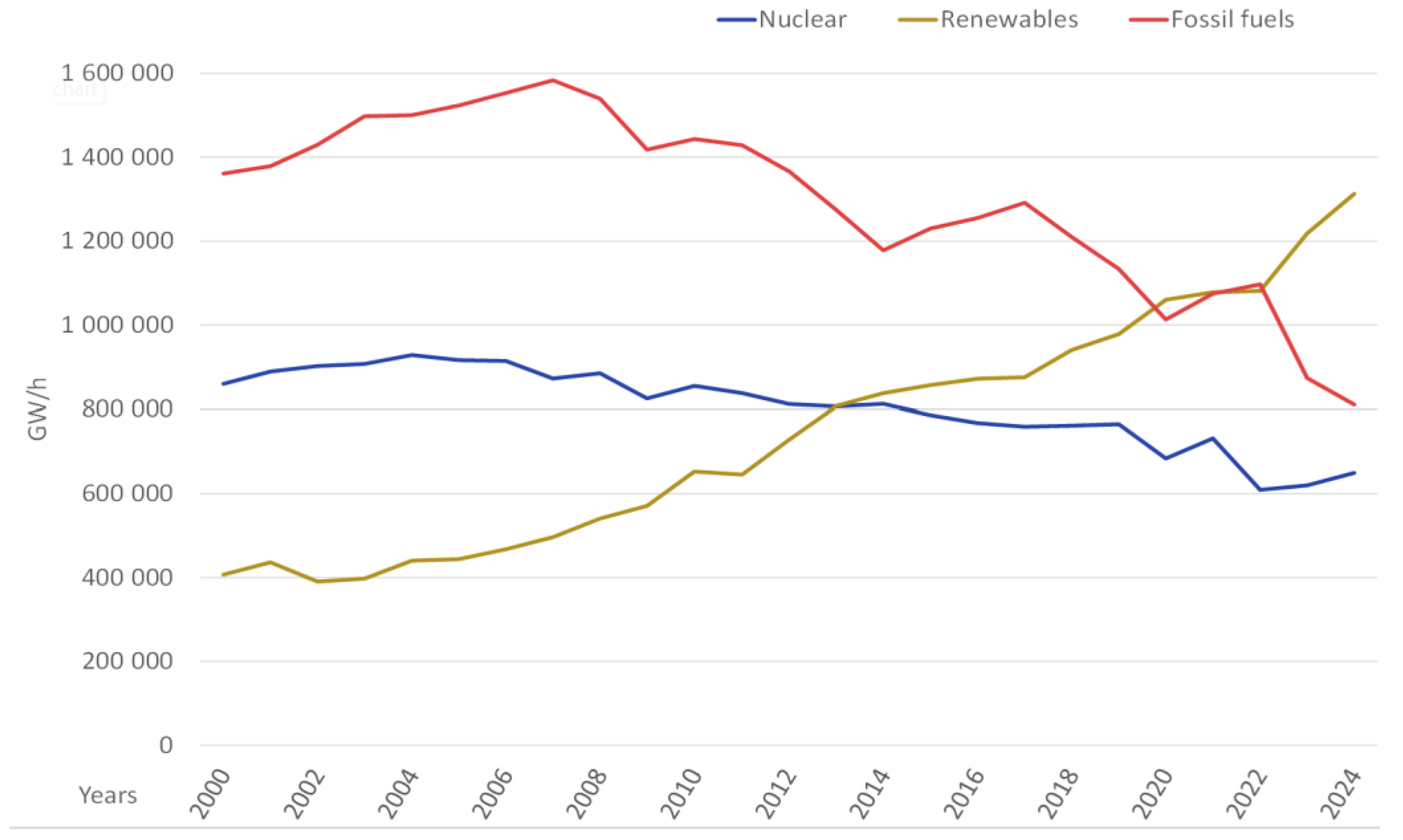
Figure 2.
Analysis of DAM using FFT and ACF for years 2023-2025.
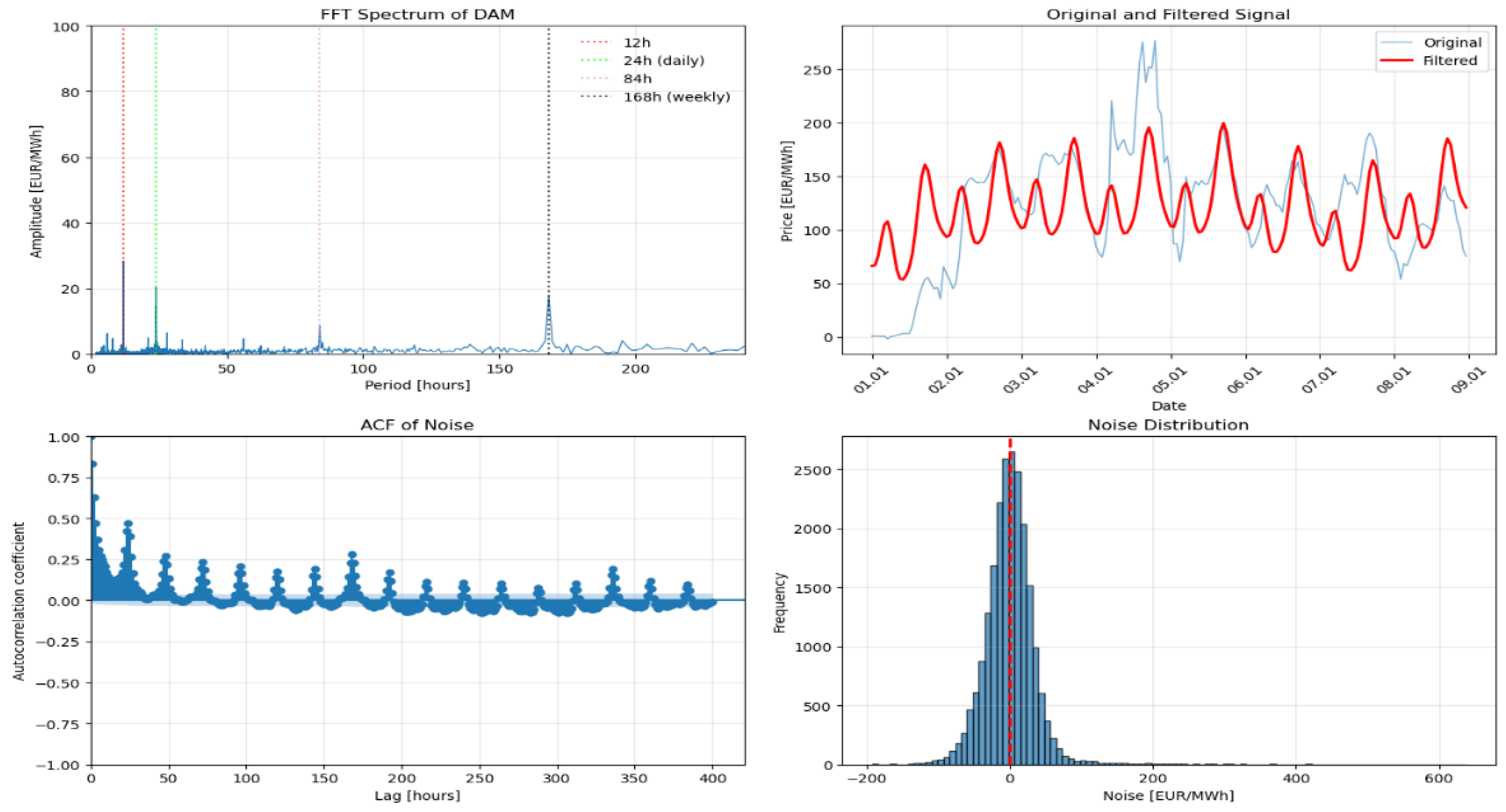
Figure 3.
Analysis of DAM using FFT and ACF for years 2020-2025.
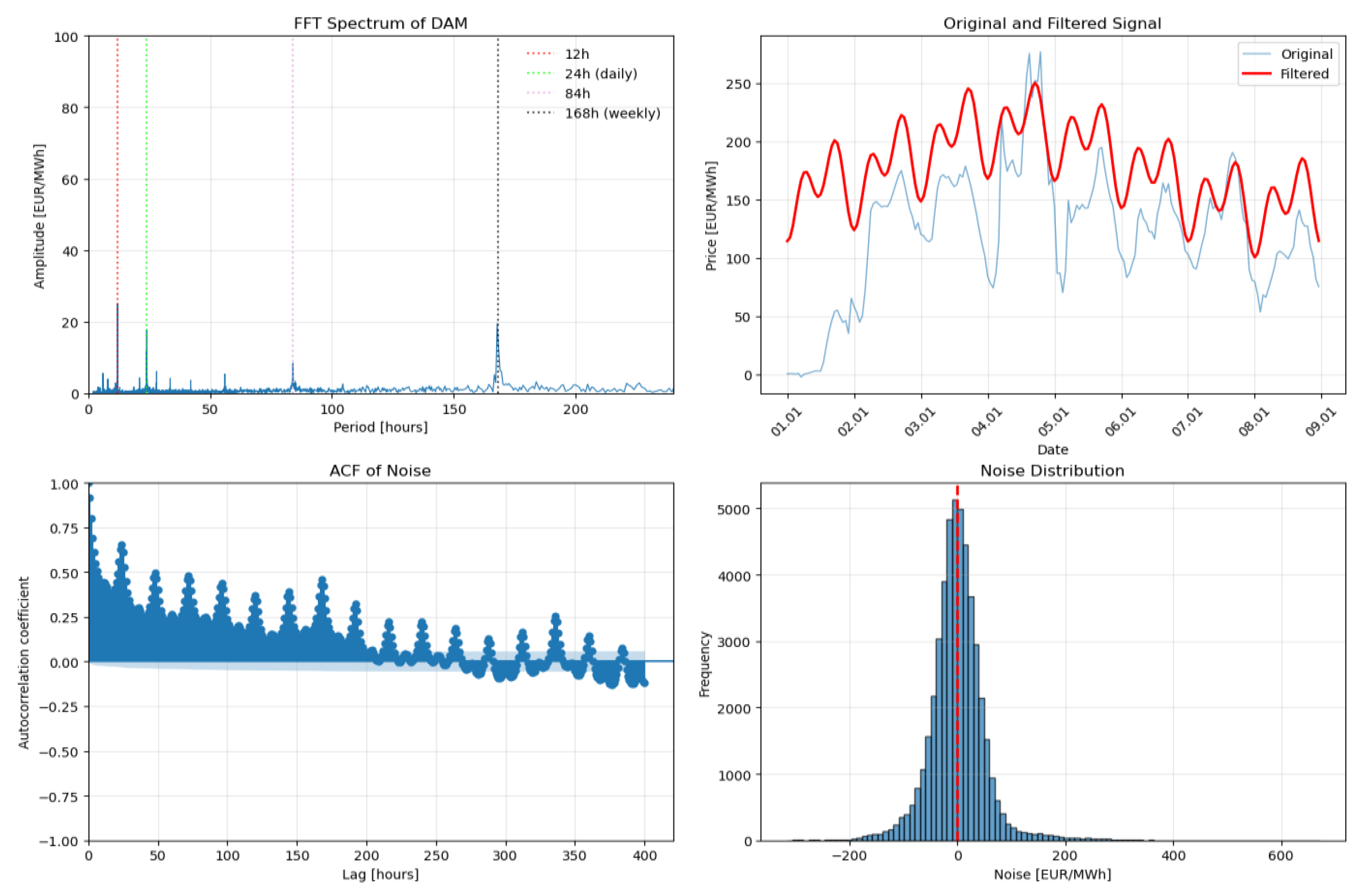
Figure 4.
Correlations of commodities.
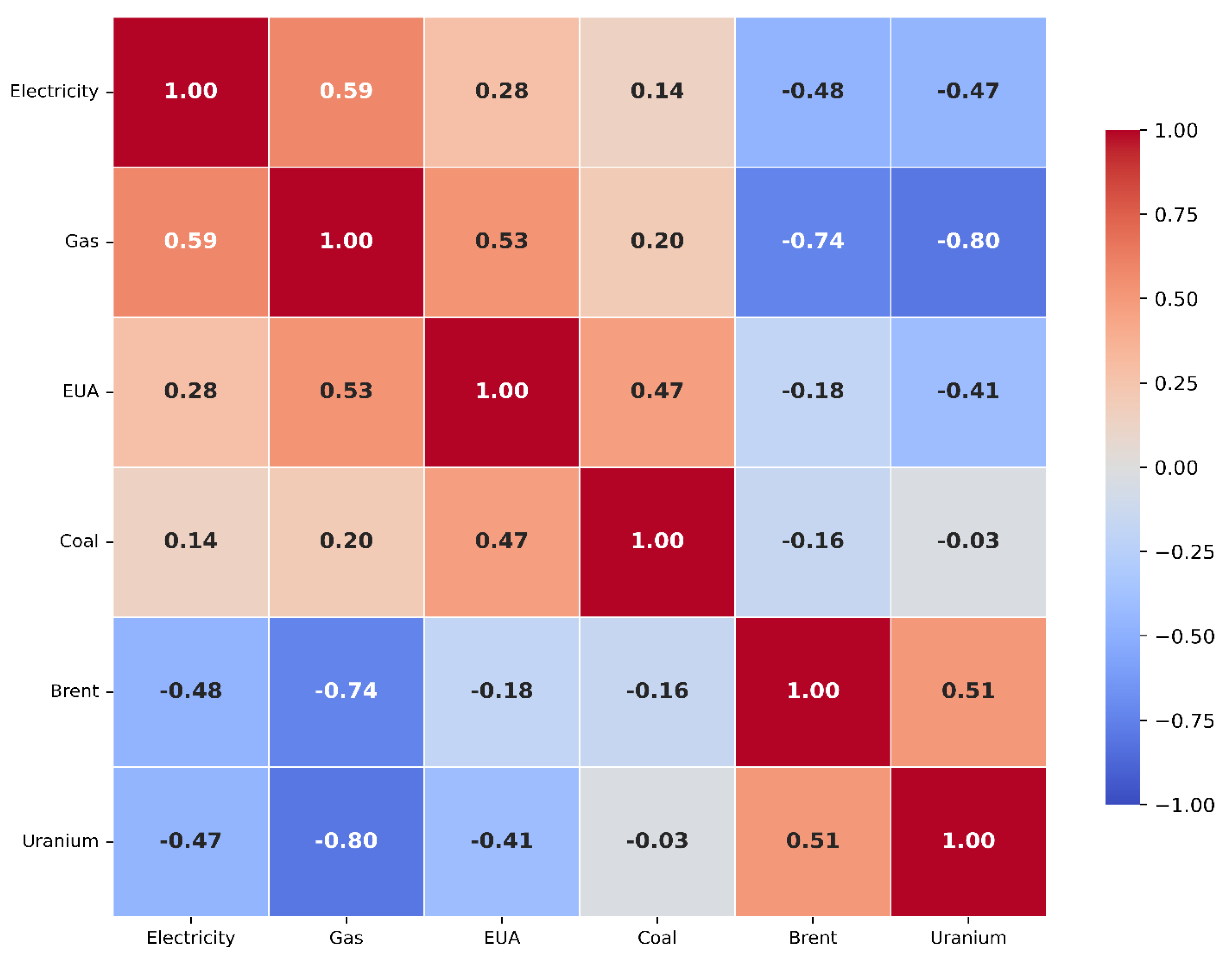
Figure 5.
Average correlation of the commodities for each hour in year.
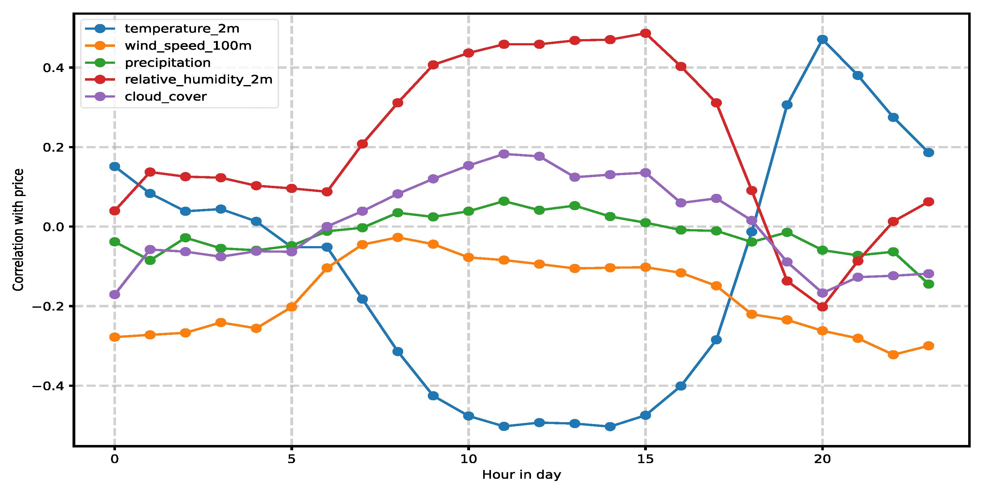
Figure 6.
Correlation of the weather dependency of price.
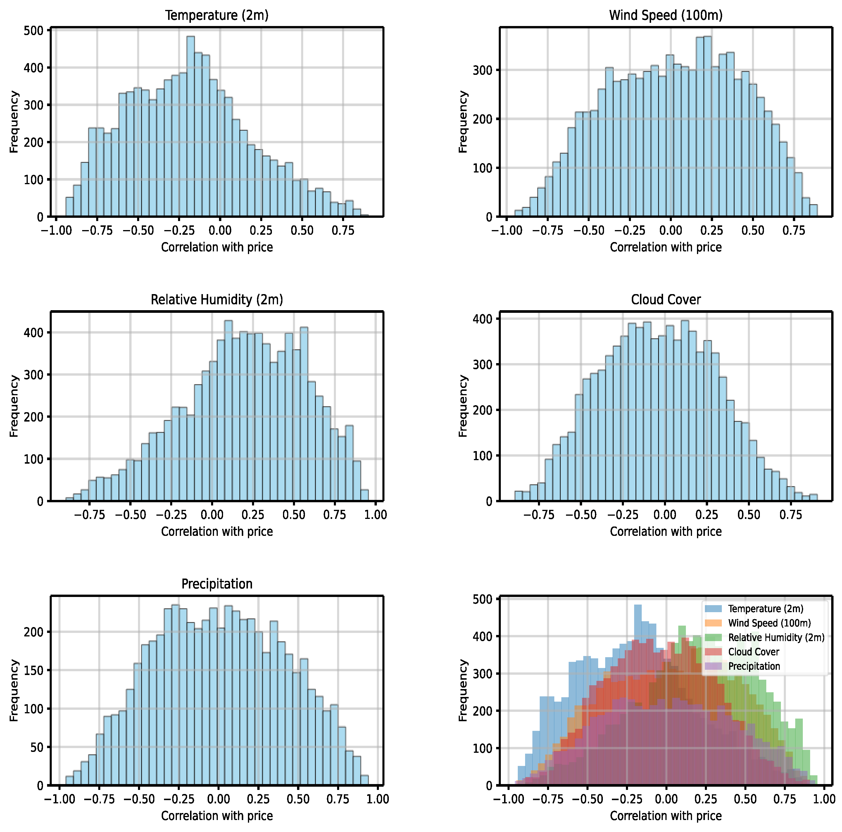
Figure 7.
Price of the day-head market trough year 2020-2025.
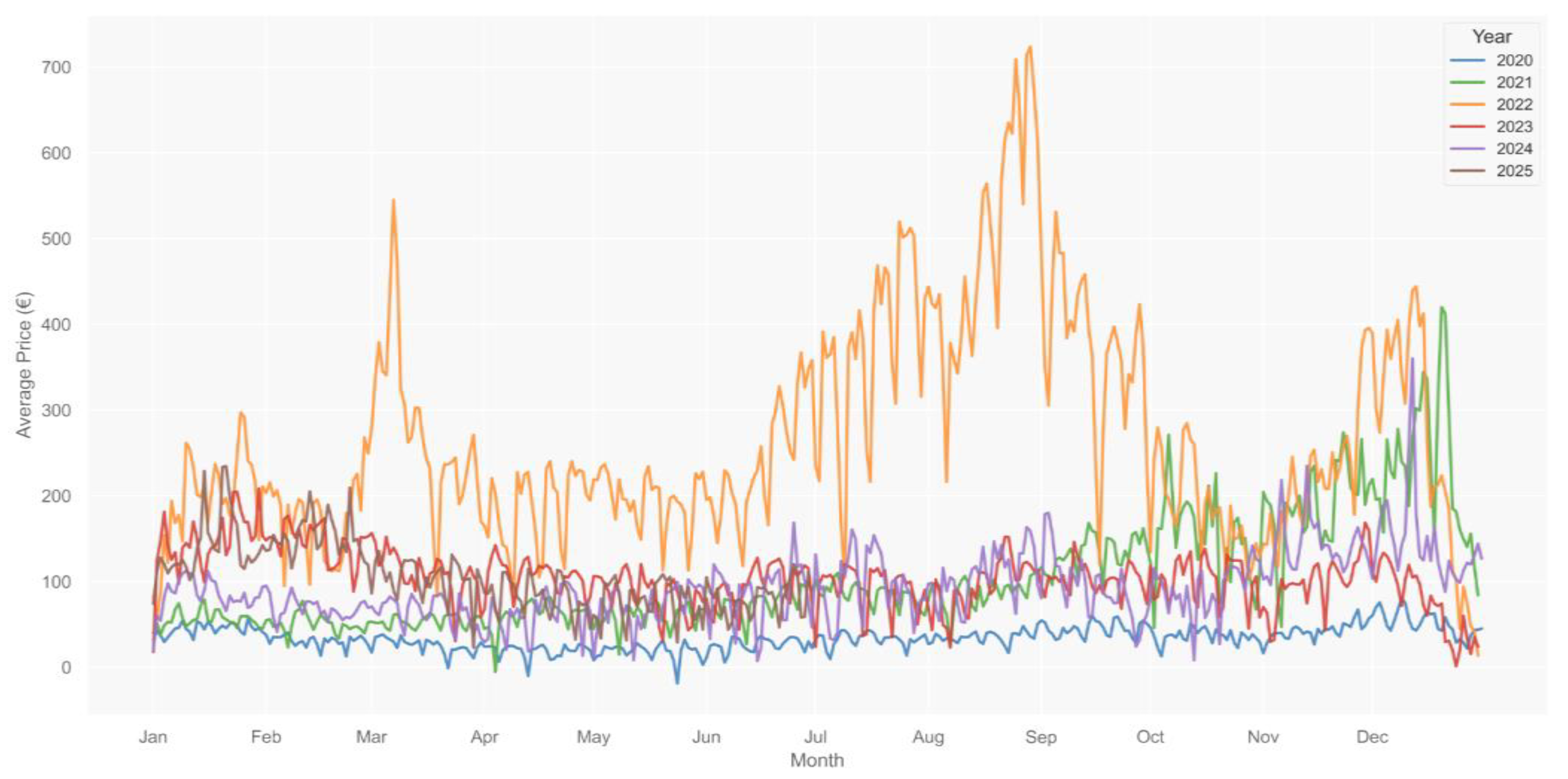
Figure 8.
Price distribution used for forecasting price.
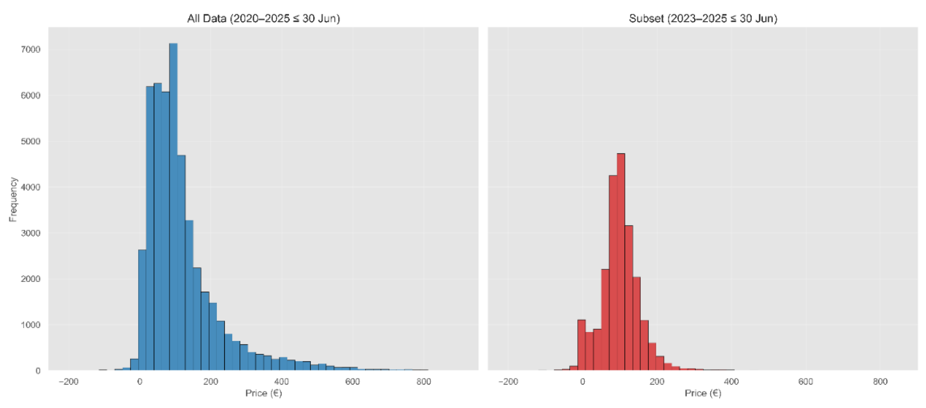
Table 2.1.
Summary of the accuracy of predictive models for short-term price prediction.
| Models | Errors | MAPE (%) | MAE (€/MWh) | RMSE (€/MWh) | ||||||||||||
| Season | Winter | Spring | Summer | Autumn | Winter | Spring | Summer | Autumn | Winter | Spring | Summer | Autumn | ||||
| LSTM | Data1 | 0.91 | 0.63 | 1.23 | 0.91 | 0.45 | 0.26 | 1.72 | 0.42 | 0.56 | 0.33 | 3.57 | 0.57 | |||
| LSTM | Data2 | 1.32 | 1.89 | 2.13 | 3.44 | 0.03 | 0.08 | 0.06 | 0.05 | 0.048 | 0.11 | 0.08 | 0.09 | |||
| Model | Errors | MAPE (%) | MAE (€/MWh) | RMSE (€/MWh) | ||||||||||||
| 1 | Data3 | 7.51 | 3.59 | 4.71 | ||||||||||||
| 2 | Data3 | 7.51 | 3.59 | 4.71 | ||||||||||||
| 3 | Data3 | 7.51 | 3.58 | 4.71 | ||||||||||||
| 4 | Data3 | 7.63 | 3.64 | 4.77 | ||||||||||||
| 1 | Data3 | 7.67 | 3.65 | 4.79 | ||||||||||||
| 2 | Data3 | 7.68 | 3.64 | 4.79 | ||||||||||||
| 3 | Data3 | 7.69 | 3.65 | 7.80 | ||||||||||||
| 4 | Data3 | 7.80 | 3.70 | 4.86 | ||||||||||||
| Model | Errors | MAPE (%) | MAE (€/MWh) | RMSE (€/MWh) | ||||||||||||
| Steps a head | 1 | 3 | 6 | 1 | 3 | 6 | 1 | 3 | 6 | |||||||
| LSTM CNN | Data4 | 20.01 | 19.10 | 21.91 | 9.05 | 12.05 | 13.64 | 0.028 | 0.033 | 0.038 | ||||||
| Seq2Seq | Data4 | 12.20 | 17.94 | 26.87 | 9.65 | 10.19 | 12.37 | 0.028 | 0.030 | 0.36 | ||||||
| Informer | Data4 | 23.01 | 22.17 | 30.67 | 12.89 | 14.25 | 13.08 | 0.029 | 0.032 | 0.031 | ||||||
| ST-Norm | Data4 | 11.90 | 19.50 | 14.76 | 7.83 | 11.53 | 10.86 | 0.02 | 0.031 | 0.030 | ||||||
| MTGNN | Data4 | 11.74 | 13.75 | 12.98 | 8.91 | 8.53 | 9.52 | 0.028 | 0.029 | 0.033 | ||||||
| ASTGCN | Data4 | 16.67 | 15.40 | 15.15 | 7.62 | 8.49 | 9.28 | 0.028 | 0.030 | 0.033 | ||||||
| MGAAL | Data4 | 11.73 | 13.61 | 14.08 | 7.70 | 9.04 | 9.74 | 0.024 | 0.026 | 0.029 | ||||||
| LSTM CNN | Data5 | 56.63 | 77.00 | 69.87 | 54.53 | 70.92 | 89.59 | 0.036 | 0.040 | 0.045 | ||||||
| Seq2Seq | Data5 | 14.73 | 28.40 | 47.26 | 52.34 | 63.54 | 70.51 | 0.033 | 0.033 | 0.04 | ||||||
| Informer | Data5 | 47.00 | 46.66 | 62.22 | 51.06 | 54.73 | 56.53 | 0.03 | 0.036 | 0.04 | ||||||
| ST-Norm | Data5 | 13.73 | 16.85 | 20.41 | 54.62 | 50.22 | 63.61 | 0.036 | 0.036 | 0.047 | ||||||
| MTGNN | Data5 | 11.07 | 14.27 | 15.95 | 40.83 | 42.77 | 48.48 | 0.024 | 0.026 | 0.037 | ||||||
| ASTGCN | Data5 | 23.33 | 21.72 | 20.91 | 52.50 | 55.46 | 58.06 | 0.036 | 0.046 | 0.046 | ||||||
| MGAAL | Data5 | 20.13 | 22.87 | 23.63 | 40.07 | 46.08 | 40.16 | 0.0297 | 0.0283 | 0.028 | ||||||
Table 4.1.
Model results for forecasting price for years 2020-2025 and 2023-2025.
| Period | Sequence length (h) | Forecast length (h) | Epoch (-) | t (s) | R2 (-) | MAE (€/MW) |
| 2020-2025 | 168 | 168 | 28 | 4447.00 | 0.44 | 33.29 |
| 168 | 84 | 56 | 5819.78 | 0.71 | 23.67 | |
| 168 | 24 | 63 | 5020.02 | 0.80 | 18.38 | |
| 168 | 12 | 25 | 1839.47 | 0.80 | 18.49 | |
| 168 | 1 | 36 | 2566.16 | 0.85 | 14.71 | |
| 84 | 84 | 51 | 3116.50 | 0.72 | 23.11 | |
| 84 | 24 | 43 | 1972.27 | 0.80 | 18.30 | |
| 84 | 12 | 46 | 1725.48 | 0.83 | 16.48 | |
| 84 | 1 | 54 | 2024.49 | 0.85 | 14.56 | |
| 24 | 24 | 23 | 346.11 | 0.77 | 19.92 | |
| 24 | 12 | 36 | 419.22 | 0.81 | 17.17 | |
| 24 | 1 | 27 | 269.22 | 0.83 | 15.62 | |
| Period | Sequence length (h) | Forecast length (h) | Epoch (-) | t (s) | R2 (-) | MAE (€/MW) |
| 2023-2025 | 168 | 168 | 57 | 4100.82 | 0.53 | 28.48 |
| 168 | 84 | 44 | 2073.68 | 0.59 | 27.52 | |
| 168 | 24 | 40 | 1576.23 | 0.75 | 20.34 | |
| 168 | 12 | 39 | 1487.36 | 0.81 | 17.55 | |
| 168 | 1 | 36 | 1191.24 | 0.87 | 13.63 | |
| 84 | 84 | 11 | 373.06 | -1.71 | 87.32 | |
| 84 | 24 | 31 | 556.39 | 0.71 | 22.76 | |
| 84 | 12 | 33 | 572.35 | 0.80 | 17.70 | |
| 84 | 1 | 22 | 361.50 | 0.85 | 14.29 | |
| 24 | 24 | 27 | 206.79 | 0.74 | 20.97 | |
| 24 | 12 | 30 | 188.07 | 0.80 | 18.49 | |
| 24 | 1 | 21 | 102.06 | 0.84 | 16.21 | |
Disclaimer/Publisher’s Note: The statements, opinions and data contained in all publications are solely those of the individual author(s) and contributor(s) and not of MDPI and/or the editor(s). MDPI and/or the editor(s) disclaim responsibility for any injury to people or property resulting from any ideas, methods, instructions or products referred to in the content. |
© 2025 by the authors. Licensee MDPI, Basel, Switzerland. This article is an open access article distributed under the terms and conditions of the Creative Commons Attribution (CC BY) license (http://creativecommons.org/licenses/by/4.0/).
Copyright: This open access article is published under a Creative Commons CC BY 4.0 license, which permit the free download, distribution, and reuse, provided that the author and preprint are cited in any reuse.


