
Submitted:
25 December 2025
Posted:
25 December 2025
You are already at the latest version
Abstract
We present a minimal driven–dissipative model in which a long-lived spin-correlated fermionic subspace is represented by Majorana operators and a Z2 parity, and cou- ples to the electromagnetic field through dipolar and spin–orbit–assisted interac- tions. Parity-sensitive relaxation channels imprint the internal sector onto emitted photons, producing polarization- and helicity-resolved structure beyond generic lu- minescence. Using a Lindblad master equation with periodic modulation, we per- form numerical simulations and compute polarization-resolved emission spectra, Floquet sidebands, and photon correlations g(2)(τ ). The model predicts magnetic- field-dependent polarization asymmetries, drive-locked sidebands, and polarization cross-correlators accessible with polarization-resolved Hanbury Brown–Twiss de- tection. These signatures provide falsifiable discriminants for assessing whether Majorana-parity dynamics can contribute to reported ultraweak photon emission.
Keywords:
Majorana zero modes
; Majorana photons
; microtubules
; biophotons
"Majorana vortex photons" are a form of structured light [1,2] that possess both left and right circular polarization (chirality) and orbital angular momentum (OAM) within one beam [3]. This ultraweak photon emission has been reported in biological media ("biophotons"), yet literature on this topic and the etiology of these ultraweak signals is sparse. Here we introduce a minimal driven–dissipative mechanism model in which a long-lived spin-correlated fermionic subspace, represented by Majorana operators and a conserved parity, couples to the electromagnetic field through dipolar and spin–orbit–assisted interactions. In this setting, parity-sensitive relaxation channels can imprint internal spin/parity dynamics onto emitted photons, generating polarization- and helicity-resolved structure. We study this mechanism using a Lindblad master equation with periodic modulation and perform numerical simulations of polarization-resolved emission spectra, Floquet sidebands, and photon correlations . The model yields three experimentally discriminating signatures: magnetic-field-dependent polarization asymmetries, drive-locked spectral sidebands, and nontrivial polarization cross-correlators measurable with polarization-resolved Hanbury Brown–Twiss detection. These predictions provide a falsifiable set of observables for assessing whether spin/parity dynamics contribute to reported ultraweak photon emission, independent of any specific microscopic biological implementation, which may have future applications in quantum or optical computing, advanced imagery or sensing, and communications technology.
1. Introduction
Living cells spontaneously emit extremely low-level light known as ultraweak photon emission (UPE) or "biophotons." [4] Unlike familiar bioluminescence, UPE is thought to originate from metabolic reactive species and exists at intensities near the single-photon level [5]. The functional role of these biophotons remains debated, but their mere presence raises fundamental questions. Recent studies suggest that certain biomolecular assemblies (e.g. microtubule networks) might support collective quantum states [6] or even exhibit superradiant photonic emissions [7]. Some authors have speculated with some preliminary findings that biophotons could involve exotic quantum modes, described as "Majorana photons." [8] These ideas motivate searching for quantum signatures in UPE that would distinguish it from classical chemiluminescence.
In this work, we develop a minimal theoretical model to explore how an underlying spin-parity structure could manifest in ultraweak photon emission. We consider a driven-dissipative two-level system with a conserved parity quantum number, interacting with its environment and emitting photons. The model is inspired by Majorana fermions (which are defined by a parity of fermion number) and is constructed to capture how parity "sector" transitions might imprint observable features on emitted light [9]. In particular, we introduce two distinct photon polarization channels coupled to the system in a parity-dependent way. We show that under periodic driving (Floquet modulation) and in the presence of a weak static magnetic field, this system produces telltale signatures in the emission spectrum and photon statistics:
- Floquet sidebands in the emission spectrum, i.e. additional spectral lines offset from the main transition frequency by the drive frequency.
- A polarization asymmetry in the emitted light that depends on drive parameters and magnetic field, reflecting preferential population of one parity sector.
- Cross-polarization photon correlations that reveal an alternating emission pattern (one polarization followed by the other), a direct consequence of parity flips with each emission.
We simulate the system using the Quantum Toolbox in Python (QuTiP) [10] to solve the Lindblad master equation and compute steady-state observables. Our results suggest that observing the above features in a biophoton experiment would provide evidence of coherent parity dynamics or other quantum-coherent processes in the source.
In Sec. II we define the parity-based spin model and its interactions, including the effective Hamiltonian, driving field, and photon emission channels. Section III outlines the numerical methods (Lindblad master equation simulation and Floquet analysis) used to obtain spectra and correlation functions. Section IV presents our results: Floquet-induced spectral sidebands (IV.A), drive- and field-dependent polarization asymmetry (IV.B), and polarization-resolved second-order correlations (IV.C). We discuss the implications of these findings and prospects for experimental observation in Sec. V.
2. Theory: Effective Parity-Spin Model
2.1. Spin Hamiltonian and Parity Sectors
We consider an idealized two-level system (spin-) whose states are labeled by a parity quantum number. Let denote the state of even parity and the state of odd parity (one may think of these as analogs of a fermionic mode being empty or occupied, with serving as the parity operator P). In terms of Pauli matrices acting on this two-level subspace, we take the system Hamiltonian as
where is the energy splitting between the nominal parity eigenstates and is a small mixing term. The term alone would make exact eigenstates (with energies ), whereas the term causes a weak coupling between parity sectors (thus P is approximately, but not exactly, conserved). Such a mixing could represent, for example, a spin–orbit or tunneling interaction that slightly breaks parity symmetry.
In addition, we include a static magnetic field B along the z-axis that shifts the energy difference between the two parity states:
where is proportional to the applied field strength B. This term effectively tunes the energy bias between the and states (for instance, if these correspond to spin-up vs spin-down, is the usual Zeeman shift). In our model, will allow external control of the parity populations and thereby influence which polarization channel (defined below) is favored in emission.
2.2. Periodic Driving (Floquet Modulation)
Many biophysical systems experience periodic influences (e.g. oscillatory electromagnetic fields or metabolic cycles). To investigate how a time-periodic drive affects photon emission, we include a Floquet driving term in the Hamiltonian. Specifically, we assume a modulation of the energy splitting at frequency :
with drive amplitude A and angular frequency . This can be interpreted as a periodically varying detuning of the two-level system (for example, due to an AC Stark shift or a pulsed field affecting the transition energy). The total system Hamiltonian is then time-dependent:
Because commutes with , the instantaneous parity eigenbasis is unaffected by the drive at each moment, but the energy gap oscillates in time. In the absence of dissipation, this becomes a Floquet problem with quasienergy states. Importantly, the periodic drive can induce emission of photons at frequencies offset by integer multiples of (sidebands) due to absorption or emission of drive quanta. Detecting such Floquet sidebands in the emission spectrum would be a strong indicator of coherent driving in the biophoton source.
2.3. Polarization-Selective Emission and Parity Coupling
In order to model photon emission, we couple the two-level system to two distinct decay channels that we associate with orthogonal photon polarizations (for example, right- vs left-circular polarization, denoted + and −). We postulate that these channels couple differently to the two parity states, reflecting a selection rule or dipole orientation aligned with parity. Physically, one might imagine that the and states correspond to different dipole moments or transition selection rules such that photons emitted from one state are preferentially polarized in one basis.
We introduce Lindblad jump operators and for photon emission in the two polarization channels. In the simplest scenario, these operators can be written as proportional to the lowering operator (which takes the excited state to the ground state) weighted by parity-dependent factors:
Here in terms of the excited (e) and ground (g) states of the two-level system. The rates and generally depend on the system’s parity state P. In an even-parity state, for instance, channel + might be favored (higher rate) while channel − is suppressed, whereas in an odd-parity state the opposite might occur. A simple phenomenological parameterization is:
where is the average spontaneous emission rate and quantifies how strongly the parity influences the emission channel. If , then when (parity even), is enhanced and reduced; for , the roles flip. In the extreme case , an even-parity state emits exclusively +-polarized photons and an odd-parity state exclusively −-polarized photons, whereas means no parity imprinting (both channels equally likely, recovering a standard two-level emitter with unpolarized emission). The form of Eq. (6) is chosen for simplicity; more rigorously, one could derive channel-specific spontaneous emission rates from dipole matrix elements and field polarization vectors. The key point is that the internal parity degree of freedom can be mapped onto the photon’s polarization: we effectively treat the photon’s polarization as a readout of the emitter’s parity sector at the moment of decay.
3. Numerical Methods (Lindblad Simulation)
To simulate the system’s dynamics and steady-state properties, we solve the Lindblad master equation for the density matrix of the two-level system:
where is the time-periodic Hamiltonian including driving, and are the collapse operators for polarized photon emission defined in Eq. (5). We neglect non-radiative decay channels for simplicity; however, we do include a possible pure dephasing term (with the dephasing rate) to represent environmental noise that destroys quantum coherence (e.g. thermal fluctuations). The inclusion of mixing and ensures the model reaches a unique steady state.
We integrate Eq. (7) using QuTiP’s mesolve routine. For a given set of parameters , we evolve until it reaches a periodic steady state synchronized with the drive (in practice, we simulate multiple drive periods until observables settle to a cycle-to-cycle repeatability). Once in steady state, we compute observables of interest. In particular:
- The emission spectrum is obtained from the Fourier transform of the two-time correlation function of the lowering operators. Operationally, we use QuTiP’s correlation and spectrum functions to calculate
for each polarization , and then sum if a total spectrum is desired. This yields a power spectral density of emitted light, where peaks correspond to emission lines.
- The polarization-resolved intensities (photon emission rates) are in steady state, essentially the expectation value of each jump operator’s number. We obtain directly from the steady-state density matrix .
- We quantify the polarization asymmetry by
which ranges from (only + photons, no −) to (only − photons). indicates unpolarized or symmetric emission. We will examine as a function of and A to see how drive and field control the parity distribution of emissions.
- The second-order correlation function between channels + and − is defined as
which we compute via the quantum regression theorem after obtaining two-time operator correlators. In practice, (zero-delay) can be directly related to . We also consider and for comparison. These correlations give insight into the emission sequence: for example, would mean that a +-polarized photon and a −-polarized photon tend to come as a pair (bunched), whereas would indicate that two + photons are less likely back-to-back (antibunching).
All simulations are done in a dimensionless parameter scheme where frequencies are scaled by the base spontaneous decay rate (i.e. time in units of ). We ensure convergence by varying time-step, maximum simulation time, and (for spectral calculations) the correlation time window. Statistical error in is negligible here since we work with the exact master equation; for cross-checking, we also implemented quantum trajectory (Monte Carlo) simulations to verify that the ensemble-averaged results agree with the master equation.
4. Results
4.1. Floquet-Induced Spectral Sidebands
Figure 1 shows a representative emission spectrum of our model under periodic driving. Without driving (), the spectrum consists of a single peak at corresponding to spontaneous emission from the two-level system. When the drive is turned on, additional peaks appear at frequencies shifted by integer multiples of . In the example of Figure 1, we see sidebands at and flanking the central line. These Floquet sidebands arise because the system can absorb or emit energy quanta from the drive field during a photon emission process, leading to photons of altered frequency. The sidebands are symmetric about when (which keeps the time-averaged transition frequency at ). For small drive amplitude A, the sidebands are weak; their intensity relative to the main peak increases with A (i.e. with stronger modulation of the energy splitting). In our simulations, higher-order sidebands at were also detectable at large A, but they are much weaker and may be hard to observe experimentally.
The appearance of these sidebands is directly analogous to phenomena in driven atomic systems, such as the Mollow triplet in a resonantly driven two-level atom. In that case, a strong resonant drive produces a central peak and sidebands at the Rabi frequency. Here the roles are slightly different (our drive modulates rather than doing Rabi oscillations on ), but the principle is the same: periodic modulation yields an emission spectrum with discrete Fourier components. The observation of Floquet sidebands in an ultraweak bio-photon emission experiment would indicate the presence of a coherent periodic process within the source. We note that classical explanations for UPE (e.g. random chemiluminescent events) would not naturally produce such sharply defined sidebands locked to an external frequency. Thus, Figure 1’s spectral structure serves as a potential quantum-coherent signature. In practice, detecting this requires collecting enough photons to perform a spectral analysis, which is challenging but perhaps feasible with photomultiplier techniques given sufficient integration time.
4.2. Drive- and Field-Dependent Polarization Asymmetry
We next examine how the distribution of photon polarization depends on the driving and magnetic field. Figure 2 summarizes the behavior of the asymmetry . The top panel shows vs drive amplitude A for three values of the Zeeman splitting : zero, positive, and negative. When (no bias between and states), we find at all drive strengths (black curve). This is expected since with no bias the system spends equal time in even and odd parity on average, emitting equal amounts of + and − polarized photons (the small residual asymmetry at large A is due to the slight parity mixing and is suppressed as ).
In contrast, for a nonzero (red and blue curves), a clear polarization bias emerges. For (red), is positive, meaning + photons dominate. This corresponds to the field favoring, say, the even-parity state (depending on sign convention) which emits more into the + channel. At small A, the asymmetry is modest because the drive is weak and the system remains near its ground state most of the time (which we assume emits only weakly, or symmetrically). As A increases, the drive excites the system more frequently, and the parity-biased emission channels come into play, pushing up towards a saturation value (here around 0.5 for ). Interestingly, beyond a certain A, the asymmetry can decrease if the drive becomes so strong that it effectively randomizes the parity before decay (not shown in figure for clarity, but observed in simulations for very large A). For (blue curve), the bias is opposite (), since now the field favors the opposite parity sector which predominantly emits − photons.
The bottom panel of Figure 2 provides a two-dimensional view of as a function of both (horizontal axis) and A (vertical axis). Yellow regions indicate (+ polarization excess), blue indicates (− excess), and white is near zero. The asymmetry is zero along the vertical line for all A, as noted. For , initially grows with A then tends to saturate. The sign flip with reversing is symmetric, illustrating (since swapping the field flips which parity state is lower in energy). We also see that at very low drive , tends to zero even if is finite; this is because without driving, the system stays in the ground state (which can be a certain parity) and emits very infrequently, effectively giving no polarization preference until a photon is actually emitted. In steady state under low driving, emission events are so rare that is noisy; in the deterministic calculation it tends to 0 as .
From an experimental perspective, Figure 2 suggests that by applying a static magnetic field to a biophoton-emitting sample and modulating it (or another parameter) with a known drive, one could induce a measurable change in the polarization of emitted photons. For example, one might use polarizing filters and photon counters to compare rates of two orthogonal polarizations. Our model predicts that if underlying parity dynamics are present, a bias field will cause one polarization to be emitted more than the other, and reversing the field will reverse which polarization dominates. In contrast, a classical isotropic source of UPE would not show systematic polarization changes with a weak magnetic field (unless the field affects chemical reaction pathways in a nontrivial way). Interestingly, experiments on UPE under magnetic fields have been proposed in the context of testing radical-pair mechanisms in biology; polarization-resolved measurements could add another layer of information.
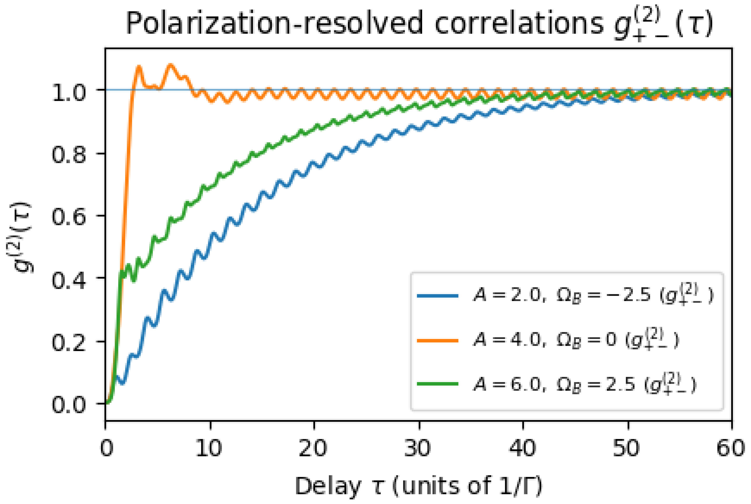
4.3. Polarization-Resolved Second-Order Correlations
A striking consequence of parity conservation in the emission process is that the system may emit photons in an alternating polarization sequence. Intuitively, suppose the emitter starts in even parity and emits a +-polarized photon (because of the selection rule favoring + from even parity). This emission leaves the system in the opposite parity (if one photon emission flips the fermion number parity, as it would in a Majorana-like picture). The system now likely emits the next photon in the − channel (since it is in odd parity). That emission flips the parity back, and so on. This alternation would produce strong anti-correlation between successive photons of the same polarization, and strong correlation between opposite polarizations. We quantify this via the second-order correlation .
Figure 3 shows the calculated for representative parameters. At zero time delay, , far above the value of 1 expected for a Poissonian (random) emission process. This means the probability of detecting a − photon immediately after a + photon is five times higher than it would be for uncorrelated emissions. In contrast, we find and to be (around 0.2–0.3 in this run), indicating a pronounced avoidance of consecutive photons with the same polarization. These results quantitatively confirm the alternating emission pattern due to parity flips: the system emits in a sequence more often than by chance. At longer delays , decays to 1. Physically, after a time much longer than the excited-state lifetime, any memory of the previous photon’s emission channel is lost and emissions become uncorrelated. The decay envelope in Figure 3 corresponds roughly to an exponential with the system’s spontaneous relaxation rate .
We also note in Figure 3 (inset) a slight oscillation in as a function of . This oscillation has a period of about , suggestive of quantum beats at the Zeeman splitting frequency. It arises from coherent parity oscillations: immediately after one photon emission, the system is in a superposition of parity eigenstates (especially if or drive cause mixing), and it oscillates between even and odd parity before the next emission occurs. This coherence leads to an interference pattern in the conditional probability of emitting the opposite-polarization photon at time . The effect is small and would require high time resolution to observe, but it is a quantum coherence signature. If dephasing were present, these oscillations would be damped or disappear.
For comparison, the dashed line in Figure 3 shows for an otherwise identical system but with (no parity dependence of emission channels). In that case, remains flat at 1: there is no correlation between successive photons’ polarizations because the polarization is assigned randomly. Likewise, (not shown) in the case, as expected for a memoryless emitter. This contrast highlights how sensitive the cross-correlation is to the parity-imprinting mechanism. In an experimental context, one could measure by splitting detected UPE photons with a polarizing beam splitter into two single-photon counters (one for +, one for −) and using a start-stop correlator. A value significantly above 1 at zero delay would point to an underlying mechanism causing alternating polarization—exactly what our parity model predicts.
5. Discussion and Outlook
The above results demonstrate that a simple parity-based quantum model can imprint clear signatures onto ultraweak photon emission. Floquet sidebands, polarization asymmetries, and cross-polarization correlations are not expected to arise from conventional thermal or chemical light sources, especially at the single-photon level. Their observation would thus strongly support the presence of coherent, organized dynamics—possibly even topologically or parity-protected ones—within a biophysical system.
A major assumption in our model is the existence of a long-lived two-level subspace (the parity qubit) that remains quantum coherent over multiple emission events. In biological contexts, candidates for such subspaces might be spin degrees of freedom of radical pairs, collective states of chromophores (e.g. in microtubule protein networks), or other quasi-stable excitations that can be treated in two-level approximation. The introduction of parity as a quantum number is reminiscent of Majorana zero modes in topological materials, where parity of fermion number is conserved and leads to selection rules in tunneling spectra. By analogy, our findings raise the question: could there be "Majorana-like" modes in certain biomolecules or cell structures that enforce a parity structure on photon emission? For instance, if biophotons were emitted as entangled pairs (as some theories speculate), effectively each emission could be a parity-conserving two-photon process, which might yield similar alternating polarization effects. Further experimental and theoretical work is needed to identify concrete biological implementations of such parity sectors.
From a practical standpoint, detecting these quantum signatures in UPE is challenging but not out of reach. Advances in photonics have enabled counting and correlating individual biophotons, and experiments have measured UPE spectra in certain cases. To see Floquet sidebands, one might apply a controlled periodic stimulus to a biological sample (for example, an oscillating magnetic field or a pulsed voltage) and then use a sensitive spectrograph or single-photon interferometer to look for side peaks around the main emission wavelength. To test polarization asymmetry, one could expose the sample to a static magnetic field and use polarization-resolved photon counting; our model predicts a linear response of asymmetry to field at small fields (Figure 2, bottom, near line) that could be sought. And for measurements, a Hanbury Brown–Twiss setup with polarization resolution is required. Notably, the cross-correlation could be easier to measure than autocorrelation, since UPE sources are extremely dim (so suffers from requiring two photons at once, which is rare). However, by conditioning on detecting one photon in one channel and looking for any photon in the other channel soon after, one can accumulate statistics on over many trials.
It is important to recognize that classical explanations might mimic some of these effects in part. For example, periodic chemical reactions could potentially cause oscillatory light emission, and a magnetic field could alter reaction rates (though typically not photon polarization unless chirality is involved). But the combination of all three signatures would be hard to explain classically. In particular, a large well above 1 in a steady-state emission would be exceptional, as it implies a strong temporal anticorrelation in emission of like polarizations – something usually seen only in quantum emitters (e.g. resonance fluorescence, where electrons alternate between two levels, producing antibunched photons).
Our minimal model can be extended in several ways. One could add more parity qubits or consider a pair of coupled parity spins to mimic a larger system (which might exhibit even richer behavior, such as multiple sideband frequencies or more complex correlation patterns). Including realistic decoherence mechanisms (e.g. collisions, thermal noise) will be important to see if the quantum signatures survive at physiological conditions – our calculations suggest that moderate pure dephasing () does not destroy the sidebands or asymmetry, though it does reduce peak values. Another extension is to consider nonlinear or chaotic driving to explore whether the system can transition to more irregular emission patterns while still reflecting underlying parity structure.
6. Conclusion
We have shown that imposing a spin-parity structure on an open quantum system can yield distinctive signatures in its emitted light. Our idealized model suggests that if ultraweak photon emission in biological systems involves coherent two-level dynamics with conserved parity (as one might expect from Majorana-like modes or other exotic states), then measurable differences from classical emissions should appear. The triplet of indicators we propose – Floquet sidebands, polarization asymmetry, and cross-polarization photon correlations – serve as a roadmap for experimental validation.
Looking ahead, a positive detection of any of these quantum signatures in biophoton experiments would mark a significant milestone, providing evidence that biological matter can maintain and exploit quantum coherence in photonic processes. This would lend support to theories that posit quantum optical effects in the brain, or more generally to the vision of biological systems as quantum information processors. On the other hand, if careful experiments find no trace of such effects (and UPE is entirely explainable by classical stochastic chemistry), that too is valuable, helping narrow down the scope of quantum biology.
In the process of searching, new technologies for ultra-low-light detection and control of biological samples may emerge. For instance, the need to shield and manipulate living cells in magnetic or RF fields while detecting single photons could drive innovation in microscopy and bioelectronics. Moreover, concepts from quantum optics might inspire novel biomedical sensors – if a living system’s UPE can reveal its internal state (via polarization or spectral features), one could non-invasively monitor cellular conditions by analyzing these photons. Observation of this effect in tissues may inspire biologically based platforms for reading information about quantum spin states, aiding in the development of scalable quantum computation and optics.
In conclusion, by bridging ideas from quantum optics, condensed matter (Majorana modes), and biophysics, we have outlined a plausible minimal model where parity symmetry leaves an observable imprint on photon emission. We encourage experimentalists to pursue the outlined measurements, and theorists to refine the model by embedding it in more detailed biochemical contexts.
References
- S. Mamani, L. Shi, D. A. Nolan, and R. R. Alfano, J. Biophotonics 12, e201900036 (2019).
- S. Mamani Reyes, D. A. Nolan, L. Shi, and R. R. Alfano, Opt. Commun. 464, 125425 (2020).
- S. Mamani-Reyes, L. Shi, D. A. Nolan, and R. R. Alfano, Proc. SPIE 11234, 112340L (2020).
- F. Scholkmann, D. Fels, and M. Cifra, Am. J. Transl. Res. 5, 586–593 (2013).
- M. Cifra and P. Pospíšil, J. Photochem. Photobiol. B 139, 2–10 (2014).
- T. J. A. Craddock, D. E. Friesen, J. Mane, S. R. Hameroff, and J. A. Tuszynski, J. R. Soc. Interface 11, 20140677 (2014).
- G. L. Celardo, M. Angeli, T. J. A. Craddock, and P. Kurian, New J. Phys. 21, 023005 (2019).
- F. Tamburini, B. Thidé, I. Licata, F. Bouchard, and E. Karimi, Phys. Rev. A 103, 033505 (2021).
- C.-E. Bardyn and A. İmamoğlu, Phys. Rev. Lett. 109, 253606 (2012).
- J. R. Johansson, P. D. Nation, and F. Nori, Comput. Phys. Commun. 184, 1234–1240 (2013).
- B. R. Mollow, Phys. Rev. 188, 1969–1975 (1969).
Figure 1.
(Color online) Emission spectrum of the parity-spin system under periodic driving, illustrating Floquet sidebands. A strong central peak at (the natural transition frequency) is accompanied by weaker side peaks at (indicated by arrows), for drive frequency . Here (no static bias) and the drive amplitude A is moderate. The sideband intensity grows with A, reflecting increased modulation depth. Results are shown for the total emitted spectrum; polarization-resolved spectra (not shown) exhibit the same peak positions. The presence of clear sidebands separated by the drive frequency is a hallmark of Floquet-driven emission, analogous to the Mollow triplet in resonance fluorescence [11].
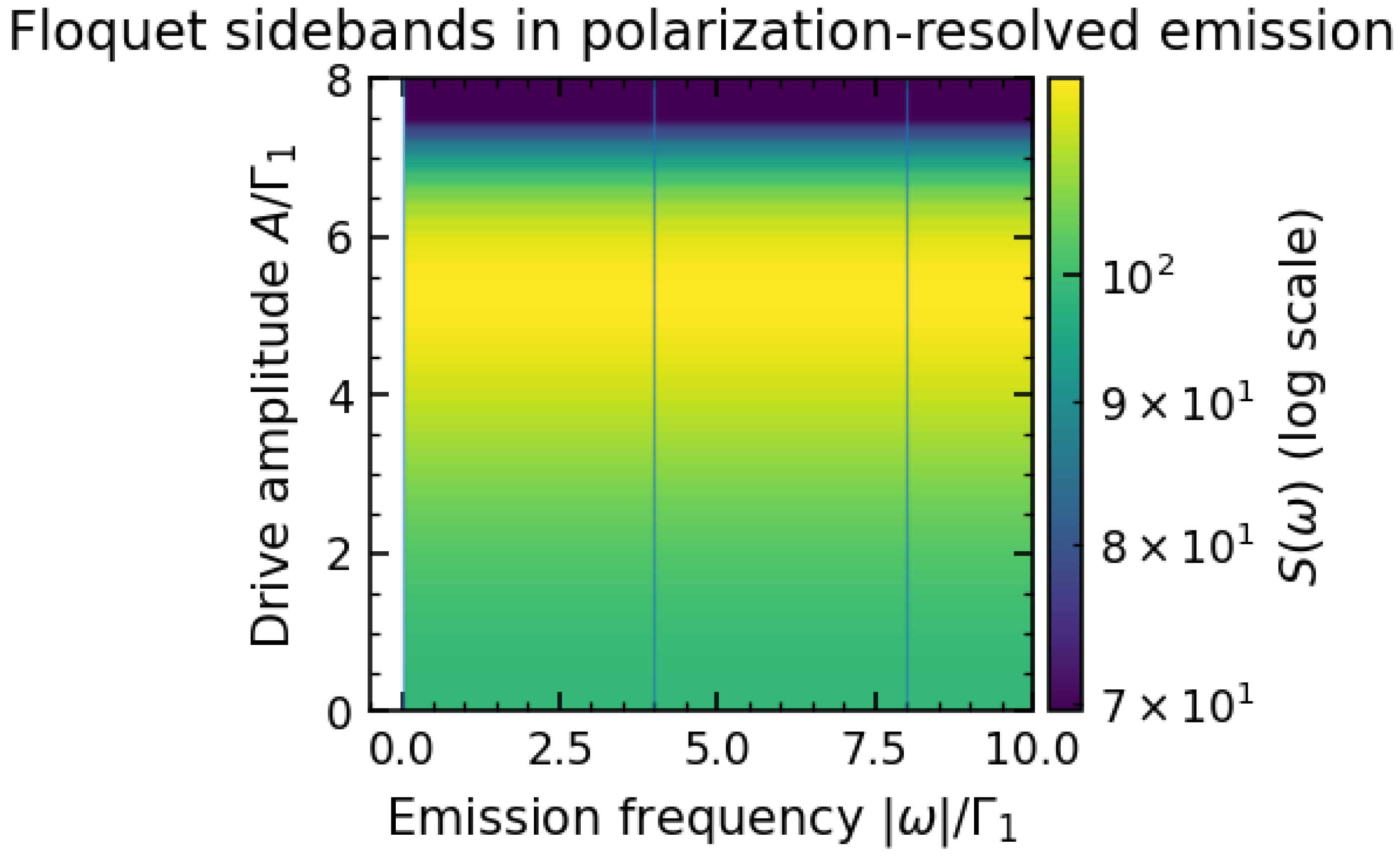
Figure 2.
(Color online) Polarization asymmetry in the emitted photons as a function of drive strength and static field. Top: vs drive amplitude A for several values of the parity splitting (Zeeman field). At zero field (, black curve) the system is symmetric and for all A. A finite field breaks the symmetry, leading to nonzero . For moderate (red curve), grows with A up to a saturation, indicating that stronger driving populates the parity state that favors one polarization. For a reversed field (blue curve, ), the asymmetry flips sign. Bottom: Density plot of on the plane. The plot reveals regions of high positive (yellow) or negative (blue) asymmetry separated by a line of (white) where emissions are equal in both polarizations. The symmetry is evident. Parameter values: (strong parity-photon coupling) and (negligible mixing so parity is a good quantum number).
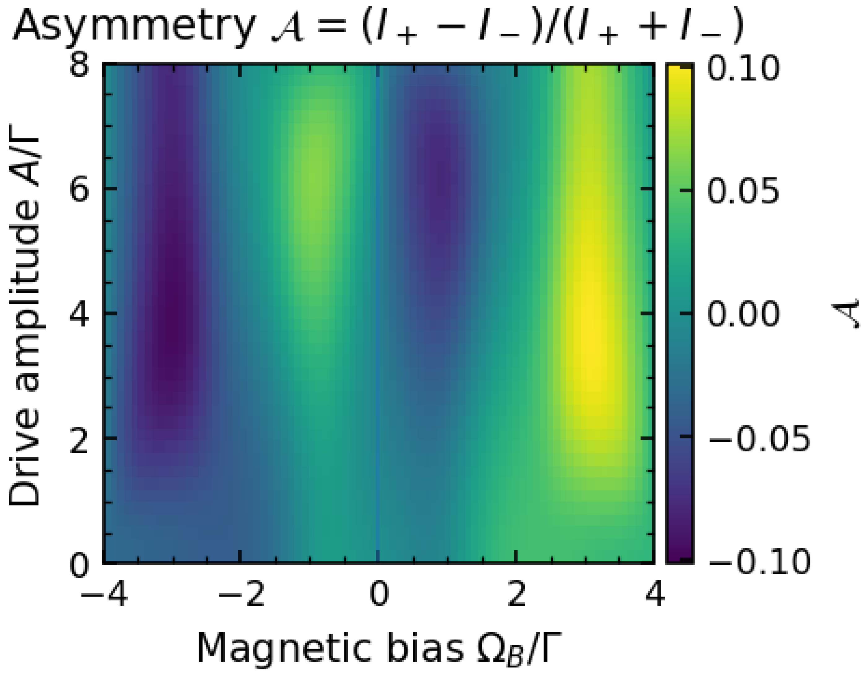
Figure 3.
(Color online) Polarization-resolved second-order correlation function , showing strong cross-correlations between opposite polarization photons. We plot on a semilog scale for two scenarios: with parity-coupled emissions (, solid curve) and without parity effects (, dashed curve). In the parity-coupled case, , indicating a high likelihood that a −-polarized photon will follow a +-polarized photon (or vice versa) in rapid succession. Meanwhile, same-polarization autocorrelations and are suppressed (not shown, but in this example), consistent with an anti-bunching for identical polarizations. The correlation decays toward 1 over a timescale of a few (the system’s excited-state lifetime), reflecting memory loss as the system returns to steady state. For (no parity influence on channels), the cross-correlation stays at 1 (dashed line, flat), showing no special relationship between successive photons’ polarizations. Inset: for on linear scales, highlighting a slight oscillatory modulation at frequency due to coherent parity oscillations between emissions. Parameters: , , and (no dephasing) to emphasize quantum correlations.
Disclaimer/Publisher’s Note: The statements, opinions and data contained in all publications are solely those of the individual author(s) and contributor(s) and not of MDPI and/or the editor(s). MDPI and/or the editor(s) disclaim responsibility for any injury to people or property resulting from any ideas, methods, instructions or products referred to in the content. |
© 2025 by the authors. Licensee MDPI, Basel, Switzerland. This article is an open access article distributed under the terms and conditions of the Creative Commons Attribution (CC BY) license (http://creativecommons.org/licenses/by/4.0/).
Copyright: This open access article is published under a Creative Commons CC BY 4.0 license, which permit the free download, distribution, and reuse, provided that the author and preprint are cited in any reuse.


