The Synchronization Latency Principle: Geometric Coherence, Informational Audit, and the Emergence of Inertia and Mass

1. Reader Contract: Assumptions, Scope, Falsifiability

We isolate what is structural (within stated assumptions) from what is model-dependent (matching and numerical outputs).

• A1 (Neighborhood choice). The substrate admits a meaningful $(1+6)$ nearest-neighbor block in three spatial dimensions.
• A2 (Audit criterion). “Matter” is defined operationally as an auditable image: certification requires a joint neighborhood constraint to be satisfied to tolerance $\epsilon \ll 1$.
• A3 (Circuit locality). One QCA timestep admits a bounded-depth decomposition into layers of disjoint two-site unitaries (plus optional on-site unitaries).
• A4 (Copy-time control parameter). A stiffness/gap-like parameter $\chi$ controls distinguishability growth in a gapped/stiff sector, enabling a conditional bound ${\tau }_{\mathrm{copy}}(\chi ,\epsilon )\gtrsim {\chi }^{-1/2}$ (constants depend on tolerance and model class).
• A5 (UV/IR matching). Any Planck calibration and any RG/FRG flow mapping UV scales to IR masses is model-dependent and must be stated as an ansatz or computed explicitly.

Falsifiable content here. Under (A1–A3) the bound $D_{\mathrm{audit}}\ge 7$ is structural. Under (A2–A4) the inequality ${\tau }_{\mathrm{mat}}\ge 7{\tau }_{\mathrm{copy}}(\chi ,\epsilon )$ is structural. Any specific IR mass value requires (A5).

2. Model Definition: QCA Dynamics and Audit Closure

2.1. Lattice, Local Degrees of Freedom, and Global Update

Let the lattice be ${\mathbb{Z}}^3$ with nearest-neighbor adjacency. Each site x carries a finite-dimensional Hilbert space

$${\mathcal{H}}_x={\mathcal{H}}_x^{\left(\mathrm{field}\right)}\otimes {\mathcal{H}}_x^{\left(\mathrm{audit}\right)}.$$

(1)

A single QCA timestep is a translation-invariant, causal (locality-preserving) unitary U acting on ${⨂}_x{\mathcal{H}}_x$[1,2,3]. We assume a depth-D circuit representation

$$U=U^{\left(D\right)}{U}^{(D-1)}\dots U^{\left(1\right)},$$

(2)

where each layer $U^{\left(k\right)}$ is a product of commuting two-site unitaries on disjoint edges (a matching), optionally interleaved with on-site unitaries.

2.2. Minimal Neighborhood Block

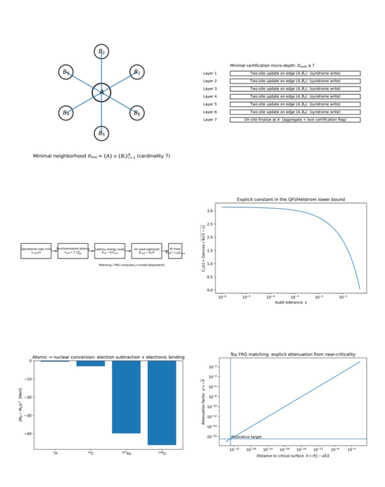
Define the $(1+6)$ neighborhood

$${\mathcal{B}}_{min}=\left\{A\right\}\cup {\left\{B_i\right\}}_{i=1}^6,\left|{\mathcal{B}}_{min}\right|=7,$$

(3)

where A is central and $B_i$ are its six axis neighbors.

2.3. Formal Audit Closure

Let ${\Pi }_{\mathrm{audit}}$ be a projector acting on ${⨂}_{x\in {\mathcal{B}}_{min}}{\mathcal{H}}_x$ defining the set of configurations judged auditable. One concrete choice is “six link constraints” between A and each neighbor $B_i$ (e.g. agreement of syndrome bits or stabilizer eigenvalues).

• Definition (certification at time t). A state ${\rho }_t$ is certified on ${\mathcal{B}}_{min}$ if

$$Tr\left({\Pi }_{\mathrm{audit}}{\rho }_t\right)\ge 1-\epsilon .$$

(4)

3. Why the Minimal Certification Depth is ${\mathit{D}}_{\mathbf{audit}}\mathbf{\ge }\mathbf{7}$ Micro-Steps

This is the first reinforcement brick: the factor 7 is a depth lower bound from locality scheduling.

3.1. Scheduling Constraint: One Edge per Layer per Site

In a layer made of disjoint two-site unitaries, any site can participate in at most one two-site gate. The central site A has six incident edges $(A,B_i)$ that must be incorporated if audit closure depends on all six neighbor relations.

3.2. Proposition (Minimal Certification Depth)

Proposition. Assume (A1–A3) and that audit closure requires incorporating information from each link $(A,B_i)$ into a joint certification (so that all six link constraints are checkable). Then

$$D_{\mathrm{audit}}\ge 6+1=7,$$

(5)

where $+1$ corresponds to an on-site “audit finalization” step (writing/locking a certification flag at A).

Proof sketch.

Each layer is a matching; site A can interact with at most one neighbor per layer. Covering the six incident edges requires at least six two-site layers. A final on-site layer aggregates/locks the audit result, hence $D_{\mathrm{audit}}\ge 7$. □

4. Operational Definition of Copy Time via Distinguishability (Helstrom)

This is the second reinforcement brick: ${\tau }_{\mathrm{copy}}$ is operational.

4.1. Distinguishability and Minimal Decision Error

Let ${\rho }_0$ be a reference state and ${\rho }_t$ the state after t micro-layers. Define the trace distance

$$\mathcal{D}({\rho }_0,{\rho }_t):={\displaystyle \frac{1}{2}}{∥{\rho }_0-{\rho }_t∥}_1.$$

(6)

For binary hypothesis testing with equal priors, the Helstrom bound gives

$$p_{\mathrm{err}}^{★}={\displaystyle \frac{1}{2}}\left(1-\mathcal{D}({\rho }_0,{\rho }_t)\right)$$

(7)

[6]. Therefore a tolerance $\epsilon$ can be implemented as a distinguishability threshold:

$$p_{\mathrm{err}}^{★}\le \epsilon ⟺\mathcal{D}({\rho }_0,{\rho }_t)\ge 1-2\epsilon .$$

(8)

4.2. Definition (copy time)

Definition. For specified $\epsilon$, define the copy time as

$${\tau }_{\mathrm{copy}}\left(\epsilon \right):=inf\left\{t\ge 0:\mathcal{D}({\rho }_0,{\rho }_t)\ge 1-2\epsilon \right\}.$$

(9)

5. Quantum-Speed-Limit Style Lower Bound and the ${\mathit{\chi }}^{\mathbf{-}\mathbf{1}\mathbf{/}\mathbf{2}}$ Scaling

This is the third reinforcement brick: ${\tau }_{\mathrm{copy}}$ admits a principled lower bound tied to information geometry.

5.1. Fidelity/Bures and Quantum Fisher Information

Let $\mathcal{F}({\rho }_0,{\rho }_t)$ be the fidelity. The Bures angle is $\theta \left(t\right)=arccos\sqrt{\mathcal{F}({\rho }_0,{\rho }_t)}$. Quantum speed-limit (QSL) inequalities relate the rate of state change to generators and information metrics [7]. In unitary families, quantum Fisher information (QFI) controls distinguishability rates; in many settings one can write a speed-limit form (schematically)

$$\theta \left(t\right)\le {\displaystyle \frac{1}{2}}{\int }_0^t\sqrt{{\mathcal{I}}_Q\left(s\right)}ds,$$

(10)

and for approximately constant QFI this yields $t\gtrsim 2\theta /\sqrt{{\mathcal{I}}_Q}$.

5.2. Mini-Section: $\chi$ in This Model (Definition, Dimension, How to Compute)

We now make $\chi$ concrete for the toy-QCA setting.

Definition (effective local generator).

Associate each micro-layer with an effective local generator K via a discrete-to-continuous parametrization:

$$U^{\left(k\right)}=exp\left(-i{K}^{\left(k\right)}\right),H_{\mathrm{eff}}^{\left(k\right)}:={\displaystyle \frac{\hslash }{{\tau }_{\mathrm{copy}}^{\left(0\right)}}}{K}^{\left(k\right)}.$$

(11)

Here $K^{\left(k\right)}$ is dimensionless and $H_{\mathrm{eff}}^{\left(k\right)}$ has dimensions of energy.

Definition (stiffness parameter $\chi$).

For a chosen reference state $|\psi \rangle$ (e.g. the pre-audit local vacuum/ready state), define

$$\chi :={\displaystyle \frac{4{Var}_{\psi }\left(H_{\mathrm{eff}}^{\left(k\right)}\right)}{{\hslash }^2}}={\displaystyle \frac{4}{{{\tau }_{\mathrm{copy}}^{\left(0\right)}}^2}}{Var}_{\psi }\left(K^{\left(k\right)}\right),$$

(12)

where ${\mathrm{Var}}_{\psi }\left(X\right)=\langle \psi |X^2|\psi \rangle -{\langle \psi \left|X\right|\psi \rangle }^2$. With this choice, $\chi$ has units of $1/{\mathrm{time}}^2$ (because $\mathrm{Var}\left(H\right)$ has units of energy² and ${\hslash }^2$ converts it to $1/{\mathrm{time}}^2$).

How to compute $\chi$ in the toy QCA.

Once the explicit gate set is chosen (Appendix A), one can:

• write each local gate as $exp(-iK)$ and identify its K;
• pick a reference $|\psi \rangle$ (commonly $|+\rangle$-type product states or the intended “ready” state);
• compute ${\mathrm{Var}}_{\psi }\left(K\right)$ analytically (for Pauli generators it is immediate) and plug into (12).

Concrete example (controlled-phase).

If the edge-interaction in layers 1–6 uses a two-qubit controlled-phase / Ising form

$$U_{AB}\left(\phi \right)=exp\left(-i{\displaystyle \frac{\phi }{2}}{Z}_A{Z}_B\right),U_{AB}\left(\phi \right)=exp\left(-i{\displaystyle \frac{\phi }{2}}{Z}_A{Z}_B\right),$$

(13)

puis $K={\displaystyle \frac{\phi }{2}}{Z}_A{Z}_B$, et pour la référence $|\psi \rangle ={|+\rangle }_A{|+\rangle }_B$, on obtient : ${\mathrm{Var}}_{\psi }\left(K\right)={\left({\displaystyle \frac{\phi }{2}}\right)}^2$. D’où :

$$\chi ={\displaystyle \frac{4}{{{\tau }_{\mathrm{copy}}^{\left(0\right)}}^2}}{\left({\displaystyle \frac{\phi }{2}}\right)}^2={\displaystyle \frac{{\phi }^2}{{{\tau }_{\mathrm{copy}}^{\left(0\right)}}^2}}.$$

(14)

So $\sqrt{\chi }=\left|\phi \right|/{\tau }_{\mathrm{copy}}^{\left(0\right)}$ is the natural “rate” set by the gate angle per micro-time.

5.3. Copy-Time Bound in Terms of $\chi$

Assume (A4) that $\chi$ controls distinguishability growth in the relevant sector so that QFI is bounded as ${\mathcal{I}}_Q\lesssim C_0\left(\epsilon \right)\chi$ (constants depend on the audit protocol and model class). Combining (10) with the certification threshold (8) yields the conditional lower bound

$${\tau }_{\mathrm{copy}}(\chi ,\epsilon )\ge C_1\left(\epsilon \right){\chi }^{-1/2}.$$

(15)

6. Synchronization Latency as an Operational Timescale

Define the matter certification time

$${\tau }_{\mathrm{mat}}=\eta {\tau }_{\mathrm{copy}}^{\left(0\right)},\eta :=7.$$

(16)

Combining (16) with (15) yields the reinforced (conditional) inequality

$${\tau }_{\mathrm{mat}}(\chi ,\epsilon )\ge 7C_1\left(\epsilon \right){\chi }^{-1/2}.$$

(17)

7. Locality Reinforcement: Lieb–Robinson and Why Synchronization is Meaningful

Locality-preserving dynamics supports an emergent causal cone; in lattice systems this is formalized by Lieb–Robinson bounds [4,5]. This supports treating audit closure as a finite-time synchronization over ${\mathcal{B}}_{min}$: influence from outside ${\mathcal{B}}_{min}$ is suppressed at short times relative to the effective light-cone.

8. Reproducible Mapping: Latency → Energy → Mass

8.1. Latency Energy Scale

Use the heuristic

$$E_{\mathrm{lat}}\sim {\displaystyle \frac{\hslash }{{\tau }_{\mathrm{mat}}}}={\displaystyle \frac{\hslash }{7{\tau }_{\mathrm{copy}}^{\left(0\right)}}}.$$

(18)

If (only if) one chooses ${\tau }_{\mathrm{copy}}^{\left(0\right)}=t$ as a UV boundary condition, then

$$E_{\mathrm{seed}}\equiv E_{\mathrm{lat}}\left(t\right)\sim {\displaystyle \frac{\hslash }{7t}}\sim {\displaystyle \frac{E_{\mathrm{Pl}}}{7}},$$

(19)

with Planck conventions from CODATA/NIST [14,15].

8.2. Explicit UV-to-IR Attenuation Factor

To connect $E_{\mathrm{seed}}$ to an IR mass $m_{\mathrm{IR}}$, define

$$m_{\mathrm{IR}}{c}^2=\rho E_{\mathrm{seed}},$$

(20)

where $\rho$ is computed by a specified matching/flow scheme (e.g. FRG) [8,9].

Context: Higgs-portal singlet scalar.

A real singlet scalar in the Higgs portal is a standard benchmark; the resonant region $m_S\approx m_h/2$ is phenomenologically special [10,11,12]. Any specific value (e.g. $58.7$ $\mathrm{G}$$\mathrm{e}\mathrm{V}$) must be presented as a model-dependent output of an explicit $\rho$ computation.

9. Reproducibility and Audit Trail (“Data vs Priors” Hard Separation)

Rule R1 (freeze priors). Fix before any comparison: neighborhood choice, audit threshold $\epsilon$, data sources (PDG/NIST/AME), and calibration convention.

• Rule R2 (no leakage). Values used as priors may not be reused as validation targets. Validation tables must cite sources and be reproducible from frozen inputs.

Maintain a minimal audit log:

AUDIT_RUN:

  script_sha256: <hash>

  inputs_sha256: <hash>

  conventions: {Planck: "reduced/unreduced", eps: 1e-6, u_to_MeV: 931.49410242}

  outputs:

    table_atomic_to_nuclear_sha256: <hash>

10. Mass-Data Hygiene: PDG vs NIST vs AME

We separate:

• Particle masses (PDG) [13],
• Atomic/isotopic masses (NIST) [18,19,20,21],
• Nuclear masses derived from atomic masses (AME practice) [16,17].

10.1. Atomic-to-Nuclear Conversion

Given a neutral-atom mass $M_A(A,Z)$, the nuclear mass is [17]

$$M_N(A,Z)=M_A(A,Z)-Z{m}_e+{\displaystyle \frac{B_e\left(Z\right)}{c^2}},$$

(21)

with electronic binding energy $B_e\left(Z\right)$. A widely used approximation is [17]

$$B_e\left(Z\right)\approx 14.4381Z^{2.39}+1.55468\times {10}^{-6}{Z}^{5.35}\mathrm{eV}.$$

(22)

11. Interpretive Summary (Reinforced)

Matter is a waiting time: a stable “image” is certified only after an audit closes over a minimal neighborhood.

Reinforcement comes from:

1.

Geometry + locality scheduling: $(1+6)$ implies $D_{\mathrm{audit}}\ge 7$ (5).

2.

Operational measurability: ${\tau }_{\mathrm{copy}}$ via Helstrom distinguishability (9).

3.

Lower-bound control: ${\tau }_{\mathrm{copy}}$ admits a QSL/QFI lower bound (15), hence ${\tau }_{\mathrm{mat}}$ obeys (17).

4.

Auditability: priors/validation separation and hash-logged artifacts prevent post-hoc tuning.

12. Outlook: Superheavy Stability as Conjecture (Scoped)

Conjecture (coherence-volume bound). If audit latency enforces an upper bound on sustainable coherence volume, then beyond a critical complexity the certification time may exceed relevant decoherence times, yielding systematically shortened lifetimes for sufficiently heavy nuclei.

• Quantitative placeholder. A working range sometimes discussed is $A\sim 310$–320, presented here only as a model-dependent placeholder until derived from explicit composite-audit dynamics and confronted with nuclear-structure systematics.

Appendix A.1. Registers

For the central site A and each neighbor $B_i$ (with $i=1,\dots ,6$), assume:

• field qubits: $f_A$ at A, and $f_{B_i}$ at $B_i$;
• audit bits at A: a 6-bit register $a_{A,i}$ (one bit per neighbor link) and a 1-bit certification flag $g_A$.

Initialize $a_{A,i}=0$ and $g_A=0$.

Appendix A.2. Edge-Syndrome Writing Layers (Layers 1–6)

For each neighbor i, define a reversible unitary $U_{A,B_i}^{\left(i\right)}$ that writes the link syndrome

$$s_i:=f_A\oplus f_{B_i}$$

into the corresponding audit bit $a_{A,i}$:

$$U_{A,B_i}^{\left(i\right)}:a_{A,i}\mapsto a_{A,i}\oplus (f_A\oplus f_{B_i}),$$

(A1)

leaving all other bits unchanged. This is a permutation on the computational basis and hence unitary.

One decomposition uses two CNOT-type updates:

1.

on-site at A: $\mathrm{CNOT}(f_A\to a_{A,i})$,

2.

two-site across the edge $(A,B_i)$: $\mathrm{CNOT}(f_{B_i}\to a_{A,i})$.

Because only one neighbor edge touches A per micro-layer (by scheduling), this respects (A3).

Appendix A.3. Audit Finalization Layer (Layer 7)

Define an on-site reversible gate $U_A^{\left(7\right)}$ that sets the certification flag if and only if all six syndromes are zero:

$$U_A^{\left(7\right)}:g_A\mapsto g_A\oplus \underset{i=1}{\overset{6}{\bigwedge }}\neg a_{A,i}.$$

(A2)

This is implementable by standard reversible logic (multi-controlled Toffoli decompositions) but the explicit decomposition is not required for the conceptual point: the finalization is an on-site aggregation step.

Appendix A.4. Audit Projector for This Toy Construction

A natural audit projector is

$${\Pi }_{\mathrm{audit}}=\left(\underset{i=1}{\overset{6}{⨂}}|0\rangle {\langle 0|}_{a_{A,i}}\right)\otimes |1\rangle {\langle 1|}_{g_A}$$

(A3)

(tensored with identity on unused degrees of freedom). In the noiseless toy setting, certification is exact on the computational basis; in noisy settings one uses tolerance $\epsilon$ as in (4).

Appendix C.1. Set-Up: Scalar Toy model and Wetterich Flow in LPA

Consider a single real scalar field in four Euclidean dimensions with an effective average action in Local Potential Approximation (LPA),

$${\Gamma }_k\left[\varphi \right]=\int d^{4}x\left[{\displaystyle \frac{1}{2}}{(\partial \varphi )}^2+V_k\left(\varphi \right)\right],V_k\left(\varphi \right)={\displaystyle \frac{1}{2}}{m}_k^2{\varphi }^2+{\displaystyle \frac{{\lambda }_k}{4!}}{\varphi }^4.$$

(A5)

The Wetterich equation reads [8,9]

$${\partial }_t{\Gamma }_k={\displaystyle \frac{1}{2}}\mathrm{Tr}\left[{\left({\Gamma }_k^{\left(2\right)}+R_k\right)}^{-1}{\partial }_t{R}_k\right],t=ln(k/\Lambda ),$$

(A6)

with IR regulator $R_k$. Using the Litim regulator $R_k\left(p\right)=(k^2-p^2)\Theta (k^2-p^2)$ yields closed-form threshold functions [?].

Define the standard dimensionless couplings

$${\tilde{m}}^2\left(k\right)={\displaystyle \frac{m_k^2}{k^2}},\tilde{\lambda }\left(k\right)={\lambda }_k,$$

(A7)

(with $\tilde{\lambda }$ dimensionless in $d=4$). In a minimal toy truncation, keep $\tilde{\lambda }$ approximately constant over the flow window (this is the toy simplification), and approximate the mass flow by the one-loop/LPA form (Litim threshold)

$${\partial }_t{\tilde{m}}^2=-2{\tilde{m}}^2+{\displaystyle \frac{\tilde{\lambda }}{16{\pi }^2}}{\displaystyle \frac{1}{1+{\tilde{m}}^2}}.$$

(A8)

In the regime $|{\tilde{m}}^2|\ll 1$, one can approximate $1/(1+{\tilde{m}}^2)\approx 1$ and obtain the linearized flow

$${\partial }_t{\tilde{m}}^2\approx -2{\tilde{m}}^2+a\tilde{\lambda },a:={\displaystyle \frac{1}{16{\pi }^2}}.$$

(A9)

Appendix C.2. Analytic Solution and Explicit ρ

Solve (A9) with UV boundary condition at $k=\Lambda$ (i.e. $t=0$):

$${\tilde{m}}^2\left(k\right)=\left({\tilde{m}}_{\Lambda }^2-{\displaystyle \frac{a\tilde{\lambda }}{2}}\right){\left({\displaystyle \frac{\Lambda }{k}}\right)}^2+{\displaystyle \frac{a\tilde{\lambda }}{2}}.$$

(A10)

The corresponding dimensionful mass is $m_k^2=k^2{\tilde{m}}^2\left(k\right)$, hence

$$m_k^2=\left({\tilde{m}}_{\Lambda }^2-{\displaystyle \frac{a\tilde{\lambda }}{2}}\right){\Lambda }^2+{\displaystyle \frac{a\tilde{\lambda }}{2}}{k}^2.$$

(A11)

Taking the IR limit $k\to 0$ gives

$$m_{\mathrm{IR}}^2=\left({\tilde{m}}_{\Lambda }^2-{\displaystyle \frac{a\tilde{\lambda }}{2}}\right){\Lambda }^2,m_{\mathrm{IR}}=\Lambda \sqrt{{\tilde{m}}_{\Lambda }^2-{\displaystyle \frac{a\tilde{\lambda }}{2}}}.$$

(A12)

Now identify the UV matching scale with the seed energy:

$$\Lambda \equiv {\displaystyle \frac{E_{\mathrm{seed}}}{c^2}}.$$

(A13)

Then (A4) and (A12) yield an explicit attenuation factor

$$\rho ={\displaystyle \frac{m_{\mathrm{IR}}{c}^2}{E_{\mathrm{seed}}}}=\sqrt{{\tilde{m}}_{\Lambda }^2-{\displaystyle \frac{a\tilde{\lambda }}{2}}}.$$

(A14)

Interpretation (why ρ can be tiny).

Equation (A14) shows that a very small $\rho$ corresponds to UV parameters lying close to the critical surface

$${\tilde{m}}_{\Lambda }^2\approx {\displaystyle \frac{a\tilde{\lambda }}{2}},$$

(A15)

i.e. near criticality. This is not a “free lunch”; it is a precise statement of what must hold in the UV to generate a much smaller IR mass in this toy truncation.

Appendix C.3. Numerical Illustration Consistent with a Higgs-Resonant Scale (Order of Magnitude)

If one uses the seed scale $E_{\mathrm{seed}}\sim E/7$ (as a boundary-condition choice) and targets $m_{\mathrm{IR}}\sim 60\mathrm{G}\mathrm{e}\mathrm{V}$, then

$${\rho }_{\mathrm{target}}\approx {\displaystyle \frac{60}{1.7\times {10}^{18}}}\sim 3.5\times {10}^{-17}.$$

(A16)

In the toy formula (A14), choosing for instance $\tilde{\lambda }=0.1$ gives $a\tilde{\lambda }/2\approx 3.17\times {10}^{-4}$, so one must set

$${\tilde{m}}_{\Lambda }^2={\displaystyle \frac{a\tilde{\lambda }}{2}}+{\rho }_{\mathrm{target}}^2\approx 3.17\times {10}^{-4}+1.2\times {10}^{-33}.$$

(A17)

The point of the example is the mechanism: the UV parameters must be fixed to (or dynamically attracted to) a near-critical surface to generate huge scale separation. In a full model, the FRG computation of $\rho$ would be replaced by a specified truncation, regulator choice, and flow integration (and the Higgs-portal sector would be included explicitly).

Appendix D.1. Step 1: Certification Threshold in Trace Distance

Let ${\rho }_0$ be a reference state and ${\rho }_t$ the state after time t (continuous) or after n micro-layers (discrete). Define trace distance $\mathcal{D}({\rho }_0,{\rho }_t)={\displaystyle \frac{1}{2}}{\parallel {\rho }_0-{\rho }_t\parallel }_1$. For binary hypothesis testing with equal priors, the Helstrom bound states [6]

$$p_{\mathrm{err}}^{★}={\displaystyle \frac{1}{2}}\left(1-\mathcal{D}({\rho }_0,{\rho }_t)\right).$$

(A19)

Requiring $p_{\mathrm{err}}^{★}\le \epsilon$ is equivalent to the threshold

$$\mathcal{D}({\rho }_0,{\rho }_t)\ge 1-2\epsilon .$$

(A20)

Appendix D.2. Step 2: Relate Trace Distance to Fidelity (Fuchs–van de Graaf)

Let $\mathcal{F}({\rho }_0,{\rho }_t)$ be the fidelity. The Fuchs–van de Graaf inequalities [??] state

$$1-\sqrt{\mathcal{F}({\rho }_0,{\rho }_t)}\le \mathcal{D}({\rho }_0,{\rho }_t)\le \sqrt{1-\mathcal{F}({\rho }_0,{\rho }_t)}.$$

(A21)

Using the upper bound in (A21) together with (A20) implies

$$1-2\epsilon \le \sqrt{1-\mathcal{F}}⟹\mathcal{F}\le 1-{(1-2\epsilon )}^2=4\epsilon (1-\epsilon ).$$

(A22)

Appendix D.3. Step 3: Bures Angle Target

Define the Bures angle

$$\theta \left(t\right):=arccos\sqrt{\mathcal{F}({\rho }_0,{\rho }_t)}\in [0,\pi /2].$$

(A23)

From (A22), certification implies

$$\theta \left(t\right)\ge {\theta }_{min}\left(\epsilon \right),{\theta }_{min}\left(\epsilon \right):=arccos\sqrt{4\epsilon (1-\epsilon )}.$$

(A24)

Appendix D.4. Step 4: QFI Speed-Limit Inequality

Quantum speed-limit results relate the rate of change of the Bures angle to the quantum Fisher information (QFI) [7]. A convenient form is

$$\theta \left(t\right)\le {\displaystyle \frac{1}{2}}{\int }_0^t\sqrt{{\mathcal{I}}_Q\left(s\right)}ds.$$

(A25)

If ${\mathcal{I}}_Q\left(s\right)\le {{\mathcal{I}}_Q}_{max}$ for $s\in [0,t]$, then (A25) yields

$$\theta \left(t\right)\le {\displaystyle \frac{t}{2}}\sqrt{{{\mathcal{I}}_Q}_{max}}⟹t\ge {\displaystyle \frac{2\theta \left(t\right)}{\sqrt{{{\mathcal{I}}_Q}_{max}}}}.$$

(A26)

Appendix D.5. Step 5: Specialize to Unitary Families and Define χ

For a unitary family ${\rho }_t=e^{-iHt/\hslash }{\rho }_0{e}^{+iHt/\hslash }$ generated by a time-independent Hamiltonian H, for pure ${\rho }_0=|\psi \rangle \langle \psi |$ one has [??]

$${\mathcal{I}}_Q={\displaystyle \frac{4{\mathrm{Var}}_{\psi }\left(H\right)}{{\hslash }^2}}={\left({\displaystyle \frac{2\Delta H}{\hslash }}\right)}^2.$$

(A27)

Motivated by this, define the stiffness parameter (as in the main text)

$$\chi :={\displaystyle \frac{4{\mathrm{Var}}_{\psi }\left(H\right)}{{\hslash }^2}},$$

(A28)

which has dimensions of $1/{\mathrm{time}}^2$. In this pure/unitary case, ${\mathcal{I}}_Q=\chi$ exactly, so we can take ${{\mathcal{I}}_Q}_{max}=\chi$.

Appendix D.6. Conclusion: Explicit Constant C 1 (ε)

Combine (A24) with (A26) and ${{\mathcal{I}}_Q}_{max}=\chi$:

$$t\ge {\displaystyle \frac{2{\theta }_{min}\left(\epsilon \right)}{\sqrt{\chi }}}=\underset{=:C_1\left(\epsilon \right)}{\underbrace{2arccos\sqrt{4\epsilon (1-\epsilon )}}}{\chi }^{-1/2}.$$

(A29)

Thus, for the operational copy-time definition as the minimal time to reach the certification threshold,

$$\tau (\chi ,\epsilon )\ge C_1\left(\epsilon \right){\chi }^{-1/2},C_1\left(\epsilon \right)=2arccos\sqrt{4\epsilon (1-\epsilon )}.$$

(A30)

Discrete micro-layer version.

If time is discrete in micro-layers of duration ${\tau }_{\mathrm{copy}}^{\left(0\right)}$, so $t=n{\tau }_{\mathrm{copy}}^{\left(0\right)}$, then

$$n\ge {\displaystyle \frac{C_1\left(\epsilon \right)}{{\tau }_{\mathrm{copy}}^{\left(0\right)}\sqrt{\chi }}},\tau \equiv n{\tau }_{\mathrm{copy}}^{\left(0\right)}\ge C_1\left(\epsilon \right){\chi }^{-1/2}.$$

(A31)

Scope note (mixed states / time-dependent generators).

For mixed states or time-dependent generators, one uses ${\mathcal{I}}_Q\left(s\right)$ along the path and (A25); the same structure holds with $\chi$ interpreted as a suitable bound on QFI over the relevant interval. The constant $C_1\left(\epsilon \right)$ remains fixed by the certification threshold via (A24).

References

- P. Arrighi, V. Nesme, and R. F. Werner, Unitarity plus causality implies localizability, J. Comput. Syst. Sci. 77, 372–378 (2011). [CrossRef]
- B. Schumacher and R. F. Werner, Reversible quantum cellular automata, arXiv: quant-ph/0405174 (2004).
- D. A. Meyer, From quantum cellular automata to quantum lattice gases, J. Stat. Phys. 85, 551–574 (1996). [CrossRef]
- E. H. Lieb and D. W. Robinson, The finite group velocity of quantum spin systems, Commun. Math. Phys. 28, 251–257 (1972). [CrossRef]
- M. B. Hastings and T. Koma, Spectral gap and exponential decay of correlations, Commun. Math. Phys. 265, 781–804 (2006). [CrossRef]
- C. W. Helstrom, Quantum Detection and Estimation Theory, Academic Press (1976).
- S. Deffner and S. Campbell, Quantum speed limits: from Heisenberg’s uncertainty principle to optimal quantum control, J. Phys. A: Math. Theor. 50, 453001 (2017). [CrossRef]
- C. Wetterich, Exact evolution equation for the effective potential, Phys. Lett. B 301, 90–94 (1993). [CrossRef]
- J. Berges, N. Tetradis, and C. Wetterich, Non-perturbative renormalization flow in quantum field theory and statistical physics, Phys. Rep. 363, 223–386 (2002). [CrossRef]
- V. Silveira and A. Zee, Scalar phantoms, Phys. Lett. B 161, 136–140 (1985). [CrossRef]
- J. McDonald, Gauge singlet scalars as cold dark matter, Phys. Rev. D 50, 3637–3649 (1994). [CrossRef]
- J. M. Cline, K. Kainulainen, P. Scott, and C. Weniger, Update on scalar singlet dark matter, Phys. Rev. D 88, 055025 (2013). [CrossRef]
- S. Navas et al. (Particle Data Group), Review of Particle Physics, Phys. Rev. D 110, 030001 (2024). [CrossRef]
- E. Tiesinga, P. J. Mohr, D. B. Newell, and B. N. Taylor, CODATA recommended values of the fundamental physical constants: 2018, Rev. Mod. Phys. 93, 025010 (2021). [CrossRef]
- NIST, CODATA Recommended Values of the Fundamental Physical Constants: 2018 (NIST SP 961, May 2019), PDF: https://physics.nist.gov/cgi-bin/cuu/Info/pdf/wall_2018.pdf.
- M. Wang, W. J. Huang, F. G. Kondev, G. Audi, and S. Naimi, The AME 2020 atomic mass evaluation (II). Tables, graphs and references, Chin. Phys. C 45, 030003 (2021). [CrossRef]
- G. Audi et al., The AME2012 atomic mass evaluation (II). Tables, graphs and references, Chin. Phys. C 36, 1603–2014 (2012). [CrossRef]
- NIST, Atomic Weights and Isotopic Compositions – Column Descriptions, https://www.nist.gov/pml/atomic-weights-and-isotopic-compositions-column-descriptions.
- NIST, Atomic Weights and Isotopic Compositions for Hydrogen, https://physics.nist.gov/cgi-bin/Compositions/stand_alone.pl?ascii=ascii&ele=H.
- NIST, Atomic Weights and Isotopic Compositions for Gold, https://physics.nist.gov/cgi-bin/Compositions/stand_alone.pl?ascii=ascii&ele=Au.
- NIST, Atomic Weights and Isotopic Compositions for Uranium, https://physics.nist.gov/cgi-bin/Compositions/stand_alone.pl?ele=U.
Disclaimer/Publisher’s Note: The statements, opinions and data contained in all publications are solely those of the individual author(s) and contributor(s) and not of MDPI and/or the editor(s). MDPI and/or the editor(s) disclaim responsibility for any injury to people or property resulting from any ideas, methods, instructions or products referred to in the content. |
© 2025 by the authors. Licensee MDPI, Basel, Switzerland. This article is an open access article distributed under the terms and conditions of the Creative Commons Attribution (CC BY) license (http://creativecommons.org/licenses/by/4.0/).
Copyright: This open access article is published under a Creative Commons CC BY 4.0 license, which permit the free download, distribution, and reuse, provided that the author and preprint are cited in any reuse.