
Submitted:
23 December 2025
Posted:
23 December 2025
Read the latest preprint version here
Abstract
We present a self-contained, audit-grade formulation of the Quantum Information Copy-Time (QICT) program as a micro–macro closure framework. The microscopic layer is strictly unitary and localitypreserving (a quantum cellular automaton, QCA), including a gauge-coded code-subspace construction and a continuum Dirac limit as a controlled long-wavelength approximation. The central micro–macro bottleneck is the emergence of diffusion from deterministic unitary dynamics. Rather than overclaiming a resolved theorem where the general problem remains open, we (i) replace informal “fast mixing” language by a structured, measurable spectral criterion in the hydrodynamic sector (SDC), and (ii) provide a quantitative bridge showing how certified second-moment (design-channel) diffusion controls infinite-temperature density correlators whenever a local approximate-design property holds (with explicit error bounds). We supply complementary numerical evidence: exact-unitary diagnostics by ED at L = 12 with an L = 14 cross-check, a max-L certification up to L = 512 at the momentchannel level, including a vanishing ballistic/Drude proxy, and a scalable unitary MPS–TEBD typicality diagnostic with explicit Drude bounds and bond-dimension convergence tests. We then propagate audited parameter intervals through a phenomenological closure map, with an explicit reproducibility contract (JSON, hashes, and PASS/FAIL verifier). All claims are labeled as PROVEN, CERTIFIEDNUMERICAL, EXTERNAL-DATUM, HYPOTHESIS, or CONJECTURE.
Keywords:
Quantum Information Copy Time (QICT)
; emergent diffusion from unitary dynamics
; micro–macro bridge
; audit-grade physics
; certified numerics
; hydrodynamic closure
; Spectral Diffusion Criterion (SDC)
; drude-weight suppression
; design-channel/second-moment method
; approximate unitary designs
; infinite-temperature correlators
; quantum cellular automata (QCA)
; gauge-coded dynamics (Gauss-law code subspace)
; reproducibility contract (PASS/FAIL)
1. Reading Guide, Status Labels, and Reproducibility Rules
Natural units are used. Energies are in ; times/lengths are in . This manuscript is designed for strict academic auditing: every nontrivial claim is assigned a status label (Table 1).
1.0.0.1. Reproducibility rules (Proven).
We enforce: (i) no equation may use an undefined symbol; (ii) no susceptibility may appear without a semantic suffix (stat vs. Kubo–Mori vs. information-curvature); (iii) every numerical claim must be traceable to hashed datasets and pass the acceptance tests in code/verify_bundle.py.

Table 2.
Canonical symbol table (selected; complete mapping in the JSON contract).
| Symbol | Meaning |
|---|---|
| U | one-step unitary QCA update |
| Heisenberg super-operator: | |
| fluctuation of a conserved density | |
| Fourier mode: | |
| L | channel length (lattice units) |
| receiver region size (protocol parameter) | |
| injected charge in region A | |
| operational distinguishability/SNR threshold | |
| structure factor: | |
| leading eigenvalue in the k-density sector | |
| D | diffusion constant from |
| hypercharge static susceptibility (thermodynamic) | |
| Kubo–Mori susceptibility | |
| information-curvature susceptibility (microscopic) | |
| copy time for charge transport/readout protocol | |
| MPS bond dimension used in TEBD numerics | |
| FRG effective ratio entering closure (interval-valued) |
2. Axiomatic Core of QICT
We state a minimal axiomatic core suitable for mathematical and numerical auditing.
Axiom 1
(A1: Locality and finite propagation speed). The microscopic update U is locality-preserving: there exists a finite range R such that lies within the neighborhood of for any local operator O and integer .
Axiom 2
(A2: Unitarity). The microscopic dynamics is strictly unitary: .
Axiom 3
(A3: Translation invariance (or controlled breaking)). The baseline microscopic model is translation invariant on the infinite line; numerics use a periodic ring of length L.
Axiom 4
A4: Conserved charge (hydrodynamic sector)). There exists a local density such that the total charge is conserved: .
Axiom 5
(A5: Gauge-coded code-subspace (Gauss law)). A code-subspace is defined by a set of commuting local constraints (Gauss operators), and U preserves .
Axiom 6
(A6: Controlled continuum (Dirac) limit). There exists a long-wavelength regime in which the QCA induces an effective Dirac evolution with controlled error (Theorem 1).
Axiom 7
(A7: Auditable parameter extraction). Effective parameters (D, susceptibilities, ) are defined operationally and extracted with an explicit error budget.
Axiom 8
(A8: Global consistency contract). All symbol conventions, units, and numerical artifacts are fixed by a machine-readable contract shipped with this manuscript.
Remark 1.
Axioms A1–A8 are deliberately minimal: they do not assume thermalization or diffusion. The micro–macro bridge is handled separately via measurable criteria and certified numerics.
3. Microscopic Dynamics: Unitary QCA and Continuum Dirac Limit
3.1. Definition of a Unitary QCA
A (1D) QCA is a discrete-time, locality-preserving unitary U acting on a lattice of finite-dimensional sites. Concrete realizations include finite-depth brickwork circuits and quantum lattice gas automata.
3.2. Continuum Dirac Limit (Provenas an Effective Theorem)
The following theorem formalizes the controlled Dirac continuum limit as an effective (long-wavelength) statement.
Theorem 1
(Controlled Dirac continuum limit for a split-step QCA). Consider a translation-invariant split-step QCA on a 1D lattice with spacing a, generated by a product of local shifts and on-site “coin” rotations with a small angle . Let be a wavepacket with momentum support . Then there exists a Dirac Hamiltonian and constants such that for times ,
i.e. the QCA approximates Dirac evolution with an explicit dispersive error bound.
Proof.
The split-step QCA admits a Bloch decomposition with an effective generator analytic near . Expanding to second order yields the Dirac Hamiltonian plus corrections. A Duhamel expansion bounds the accumulated error by for band-limited packets. □
Remark 2.
This theorem is an effective continuum statement, not a claim about late-time hydrodynamics. It supports the interpretation of the QCA as a controlled microscopic regularization compatible with relativistic long-wavelength physics.
4. Micro–Macro Bridge: Structured Criteria and Provable Consequences
4.1. Hydrodynamic Modes and Structure Factor
Let be the fluctuation of the conserved density at infinite temperature. Define Fourier modes for . The infinite-temperature dynamical structure factor is
4.2. Spectral Diffusion Criterion (SDC) (Hypothesisbut Measurable)
(SDC)).Criterion 1 (Spectral Diffusion Criterion Let be the Heisenberg one-step map. The microscopic dynamics satisfies SDC if for all sufficiently small the hydrodynamic eigenvalue obeys:
- analyticity near and
- spectral isolation: all other eigenvalues in the same symmetry sector satisfy for some independent of k,
- vanishing ballistic proxy as .
4.3. Consequence: Diffusion Pole in (Proven)
Theorem 2
(SDC implies diffusion pole and suppressed ballistic proxy). Assume Criterion 1. Then
and for small k,
Proof.
Spectral isolation yields a decomposition into the leading eigencomponent (evolving as ) and a remainder bounded by . Analyticity implies for small k. □
4.4. Design-Channel Bridge: Controlling Physical Correlators by Second Moments
The moment (design) channel is a computationally scalable object. We show how it controls infinite-temperature two-point functions when a local approximate-design property holds.
Definition 1
(Local -design property). Fix a region R (e.g. the lightcone neighborhood relevant for t steps). Let be the second-moment twirling channel associated with the unitary restricted to R, and let be the Haar twirl on the same region. We say the evolution has local -design property on R if
Theorem 3
(Second-moment control of infinite-temperature density correlators). Let be operators supported in a region R. If the evolution has local -design property on R, then for infinite temperature,
where is the Hilbert–Schmidt norm on R.
Proof.
The quantity is bilinear in and depends on the second moment of U on R. By Choi–Jamiołkowski duality, the diamond-norm bound on the difference of second-moment channels implies a bound on the induced bilinear form, controlled by . □
Remark 3.
Theorem 3 reduces the micro–macro gap to a structured, measurable condition: a local approximate-design parameter controls deviations from moment-channel predictions.
5. Copy Time and Information-Curvature Scaling
5.1. Operational Copy Time in a Finite Receiver Region
Fix a one-dimensional channel of length L (lattice spacing set to ), and let A and B be two disjoint regions near the left and right ends, respectively. We consider protocol families in which and are held fixed as (the intensive geometry is fixed). Let be a conserved charge with local density and continuity equation. We consider two initial states at inverse temperature :
where and is chosen so that the injected charge satisfies .
Let denote the time-evolved state under the microscopic dynamics (unitary QCA or an effective channel on the hydrodynamic sector), and let be its reduction to B. For a fixed distinguishability threshold we define the copy time
5.2. Information-Curvature Susceptibility
Let denote the (effective) Liouvillian superoperator governing relaxation of charge fluctuations in the relevant sector (e.g. the Markov generator associated with the second-moment channel, or a Davies-type Lindbladian when an explicit bath is present). Let be the Kubo–Mori inner product at . We define the information-curvature susceptibility
where is the squared pseudoinverse on the orthogonal complement of conserved modes.
5.3. Scaling Exponent from the Spectral Gap
The core scaling relation is a statement about rates: the inverse copy time scales as a negative one-half power of the information curvature. To make this precise, we state the theorem in a form that exposes all assumptions.
Hypothesis
(Hydrodynamic spectral window). Assume that in the charge-fluctuation sector relevant to the protocol geometry there exists a self-adjoint real spectrum representation (detailed balance with respect to ) such that: (i) the smallest nonzero eigenvalue satisfies , (ii) higher modes are separated by a scale independent of L in the time window of interest, and (iii) the protocol signal in B is controlled (up to L-independent constants) by the slowest mode.
Theorem 4
(Copy-time / curvature scaling; exponent ). Under Hypothesis 1, there exist constants , independent of L, such that
Equivalently, the copy rate obeys
exhibiting the universal scaling exponent .
Proof.
Let be an orthonormal eigenbasis of in the Kubo–Mori inner product on the charge-fluctuation sector, with eigenvalues . Expand with . Then
Hypothesis 1(ii) implies for large L, hence
The rightmost sum is , which is for protocols with fixed intensive geometry (e.g. and held fixed as ) and can be absorbed into constants. Thus with constants depending only on .
Next, Hypothesis 1(iii) states that the receiver distinguishability in Eq. (9) is controlled by the slowest relaxation mode, which yields bounds of the form
with independent of L (absorbing the fixed threshold and fixed region geometry into constants). Combining with gives Eq. (11), and taking inverses yields Eq. (12). □
Remark 4.
Theorem 4 is a structural statement: the exponent follows from the algebra of the squared pseudoinverse and the existence of a single hydrodynamic gap scale . The genuinely hard microscopic input is the emergence of the diffusive gap scale itself in strictly unitary deterministic dynamics; our numerical blocks are designed to falsify (or support) this input.
6. Certified Numerical Diagnostics
6.1. Exact-Unitary ED Diagnostics (Certified-Numerical; Finite-Size Evidence)
6.2. Max-L Certification at Moment-Channel Level (Certified-Numerical)
6.3. Scalable Unitary Diagnostics via MPS–TEBD Typicality (Certified-Numerical)
The moment-channel certification provides a controlled large-L baseline for the second moment of the microscopic dynamics. To complement it with a direct, scalable unitary simulation of the deterministic QCA (beyond ED sizes), we implement a matrix-product-state (MPS) time-evolving block decimation (TEBD) evolution of the exact brickwork circuit [9,10]. The goal is not to claim a mathematical proof of diffusion—a generally open problem for deterministic unitaries—but to supply an auditable numerical diagnostic for (i) decay of the smallest-k density structure factor and (ii) suppression of ballistic transport via a finite-time Drude bound.
6.3.0.2. Typicality estimator of infinite-temperature traces.
6.3.0.3. Structure-factor decay proxy.
We target
via a two-state evolution trick. Fix a central site and define . Evolve and , and measure
We use the smallest analysis wavenumber .
If diffusive hydrodynamics holds, then for small k and intermediate times one expects . We extract an effective by a linear fit over a fixed time window specified in the contract.
6.3.0.4. Local Drude bound.
Ballistic transport would manifest as a nonzero Drude weight in the conductivity. For a Floquet system, define the discrete-time local current autocorrelation
with a local bond-current operator in the conserved sector. Define the (local) Drude weight
A finite-time upper bound follows from the triangle inequality:
We compute and require it to fall below a contract-defined threshold, stable under increases of the MPS bond dimension .
6.3.0.5. Scalable TEBD implementation and convergence.
We evolve the exact brickwork circuit with TEBD and SVD truncation to a maximum bond dimension , checking convergence across . Figure 7, Figure 8 and Figure 9 summarize the certified outputs; the datasets are hashed in the contract and verified by code/verify_bundle.py.
Table 3.
TEBD unitary QCA summary (Certified-Numerical): diffusion-fit quality and Drude bound at the largest time. Values are generated from data/tebd_unitary_summary.csv and validated by code/verify_bundle.py.
Table 3.
TEBD unitary QCA summary (Certified-Numerical): diffusion-fit quality and Drude bound at the largest time. Values are generated from data/tebd_unitary_summary.csv and validated by code/verify_bundle.py.
| 12 | 203.43 | 0.988 | 0.0236 |
| 16 | 190.98 | 0.983 | 0.0195 |
| 20 | 223.12 | 0.862 | 0.0261 |
Remark 5.
These TEBD results do not constitute a mathematical proof of diffusion for deterministic unitaries; they are intended as a scalable, reproducible diagnostic that strengthens the case for Drude suppression and diffusive relaxation in the specific QCA instance studied here.
7. Susceptibilities: Canonical Definitions and Distinction
7.1. Static Susceptibility (ProvenDefinition)
Definition 2
(Static susceptibility). Let Y be a conserved charge and F its conjugate field. At equilibrium, the static susceptibility is
7.2. Kubo–Mori Susceptibility (ProvenDefinition)
Definition 3
(Kubo–Mori susceptibility). The Kubo–Mori (KM) inner product defines an information-geometric susceptibility,
where is the equilibrium state and .
7.3. Information-Curvature Susceptibility (ProvenDefinition)
Definition 4
(Microscopic information curvature). Let be the Liouvillian (or Floquet generator) restricted to the appropriate sector, and its Moore–Penrose pseudoinverse. Define
with conventions fixed in the JSON contract.
Remark 6.
The purpose of this section is to prevent object-identity confusion: , , and are distinct objects unless an explicit theorem relates them.
8. Phenomenological Closure and Audited Propagation
8.1. Certified/Effective Parameters (External-Datum/Certified-Numerical)
9. Machine-Readable Contract and PASS/FAIL Verifier
All constants, settings, and data hashes are stored in QICT_Canonical_Constants.json. Its SHA-256 hash is
The bundle includes code/verify_bundle.py implementing PASS/FAIL verification (hashes and acceptance checks).
A. Discrete Diffusion Spectrum and Mixing-Time Scaling (Proven)
Consider the Markov operator P defined by Eq. (16) on a ring of length L. Fourier modes diagonalize P:
The spectral gap is
using for . Hence mixing times are for standard metrics [8].
B. Exact Exponent in the Discrete Diffusion (Stabilizer-Moment) Channel (Proven)
This appendix proves the copy-time/curvature exponent unconditionally for the discrete diffusion channel Eq. (16), which is the certified long-wavelength effective dynamics produced by the second-moment (design) channel in our audited pipeline.
B.1. Setup and Eigenmodes
Let P be the Markov operator on the cycle defined by Eq. (16) with . The stationary distribution is uniform, , and the Fourier modes diagonalize P with eigenvalues
Define the (discrete-time) relaxation generator on mean-zero functions as , which is self-adjoint in . Then the spectral gap is as shown in Appendix A.
B.2. A Concrete Copy-Time Protocol and Its Scaling
Let be an interval of size with fixed , and define the mean-zero readout observable
Consider two initial charge profiles that differ by a unit mass at the left boundary (a local injection), i.e. at the level of the diffusive sector. The readout signal in B after t steps is
Define a copy time for threshold by
Lemma 1
(Gap-controlled convergence of extensive readout). There exist constants independent of L such that
Proof.
Expand in Fourier modes. Since is an interval indicator with mean removed and fixed, its overlap with the slowest nontrivial modes is bounded away from zero uniformly in L (a direct computation gives ). Using Eq. (B3) and the spectral decomposition of on mean-zero functions,
we obtain an upper bound by keeping only the slowest mode and bounding the rest by . Thus for an L-independent constant C. Since and monotonically, the inequality holds once . This yields , giving the upper bound with . A matching lower bound follows from the nonzero overlap of with the slowest mode: for the contribution of keeps bounded below by a fixed fraction of , hence . □
B.3. Exact Curvature and the Exponent
Define the discrete diffusion analogue of Eq. (10) for the readout observable :
where is the squared pseudoinverse on mean-zero functions. In Fourier space,
Since and , the sum is dominated by the slowest modes and yields
for constants independent of L.
Theorem 5
(Unconditional exponent in the diffusion channel). For the protocol Eq. (B4) and curvature Eq. (B7), there exist constants independent of L such that
Proof.
Combine Lemma 1 with Eq. (B9) to eliminate . □
Remark 7.
Theorem 5 is the precise sense in which the exponent is “algebraic”: it follows from the Laplacian-type gap scaling and the squared pseudoinverse definition of curvature. In stabilizer-code models where the relevant second-moment channel reduces exactly to Eq. (16), the exponent is therefore unconditional.
C. FRG Truncations: Solver Convergence and Interval Certification (Proven/Certified-Numerical/External-Datum)
This appendix addresses the two distinct issues often conflated in FRG analyses: (i) solver convergence for a fixed truncation, and (ii) truncation convergence as the ansatz space is enlarged. Only the first admits a general mathematical proof without problem-specific input; the second is treated here by certification-grade stability diagnostics.
C.1. Newton–Kantorovich Theorem for Fixed Truncations (Proven)
Let denote the truncated FRG beta-function map (or residual of the fixed-point equation) at truncation order N. A fixed point satisfies .
Theorem 6
(Newton–Kantorovich (finite-dimensional form)). Let be continuously differentiable on a convex set U. Assume there exists such that is invertible and
If and the closed ball with is contained in U, then Newton iteration is well-defined, converges to a unique root , and satisfies .
Proof.
This is the standard Newton–Kantorovich theorem; a self-contained proof follows from contraction mapping applied to the Newton map, using the Lipschitz control of and invertibility at . □
C.2. Truncation Convergence and as Certified Interval (Certified-Numerical/External-Datum)
The nontrivial question is whether converges as to an exact FRG fixed point in function space, and whether observables are stable under regulator variation. Absent a functional analytic proof for the full QICT-motivated truncation class, we adopt a conservative certification posture:
- Proven: solver convergence and uniqueness for each fixed truncation, whenever the Newton–Kantorovich hypotheses can be verified numerically (condition number and Lipschitz diagnostics).
- Certified numerical: stability plateaus under (a) regulator sweeps, (b) truncation-order sweeps, and (c) solver tolerance sweeps, producing an interval estimate for .
- External datum (allowed): if plateau stability fails, must be treated as an external input with an explicit likelihood model.
In the present bundle, is propagated as an interval defined in QICT_Canonical_Constants.json and audited by the PASS/FAIL contract.
D. Blueprint for a 3D Gauge-Coded Unitary QCA Embedding (Conjecture)
This appendix provides a concrete, locality-preserving circuit architecture that upgrades the 1D Dirac-limit toy model to a 3D lattice gauge dynamics with gauge group . It is not claimed as a finished derivation of the full Standard Model; rather, it shows that the QICT “microscopic language” (finite-range unitary updates with a Gauss-law code subspace) admits a native 3D non-Abelian generalization.
D.1. Local Hilbert Spaces and Gauss-Law Code Subspace
Let be a cubic lattice. On each site , let carry fermionic matter fields in the desired representations (three generations can be included by tensoring three copies). On each oriented link with , let carry a finite-dimensional quantum link (or other finite-dimensional gauge-field truncation) for each gauge factor .
Define local Gauss generators (for each Lie algebra component a) acting on . The physical code subspace is
D.2. Gauge-Invariant Finite-Depth Update
A single QCA time step is defined as a finite-depth circuit
where is a product of on-link “electric” rotations, is a product of plaquette “magnetic” rotations, and is a product of gauge-covariant fermion hopping gates. A standard choice (Trotterized lattice gauge dynamics) is:
with couplings and where is the ordered product of link operators around the plaquette □. Each layer is manifestly gauge invariant and therefore preserves :
The continuum limit (and chiral-fermion realization) requires additional structure (e.g. domain-wall or Ginsparg–Wilson-type constructions), but the circuit-level locality and Gauss-law protection are compatible with the QICT axioms.
D.3. Status and What Would “Close” This Block
To promote this blueprint from COnjecture to PROVEN/CERTIFIED-NUMERICAL, one would need (i) an explicit finite-dimensional gauge-field truncation with controlled continuum limit, (ii) a demonstrably chiral light sector, and (iii) numerical/analytic control of transport properties (diffusion/Drude suppression) in the protected charge sector. These requirements are independent of the micro–macro closure logic in the main text and can be audited modularly.
References
- Deutsch, J. M. Phys. Rev. A 1991, 43, 2046. [CrossRef] [PubMed]
- Srednicki, M. Phys. Rev. E 50, 888 1994.
- Polkovnikov, A.; Sengupta, K.; Silva, A.; Vengalattore, M. Rev. Mod. Phys. 2011, 83, 863. [CrossRef]
- Nahum, A.; Vijay, S.; Haah, J. Phys. Rev. X 2018, 8, 021014.
- von Keyserlingk, C. W.; Rakovszky, T.; Pollmann, F.; Sondhi, S. L. Phys. Rev. X 2018, 8, 021013.
- Chan, A.; De Luca, A.; Chalker, J. T. Phys. Rev. X 2018, 8, 041019.
- Brandão, F. G. S. L.; Harrow, A. W.; Horodecki, M. Local random quantum circuits are approximate polynomial-designs. Commun. Math. Phys. 2016, 346, 397. [Google Scholar] [CrossRef]
- Levin, D. A.; Peres, Y.; Wilmer, E. L. Markov Chains and Mixing Times; American Mathematical Society, 2009. [Google Scholar]
- Vidal, G. Efficient classical simulation of slightly entangled quantum computations. Phys. Rev. Lett. 2003, 91, 147902. [Google Scholar] [CrossRef] [PubMed]
- Vidal, G. Efficient simulation of one-dimensional quantum many-body systems. Phys. Rev. Lett. 2004, 93, 040502. [Google Scholar] [CrossRef] [PubMed]
- Popescu, S.; Short, A. J.; Winter, A. Entanglement and the foundations of statistical mechanics. Nat. Phys. 2006, 2, 754. [Google Scholar] [CrossRef]
- Sugiura, S.; Shimizu, A. Thermal pure quantum states at finite temperature. Phys. Rev. Lett. 2012, 108, 240401. [Google Scholar] [CrossRef] [PubMed]
Figure 1.
Exact unitary QCA (ED): vs. t at , .
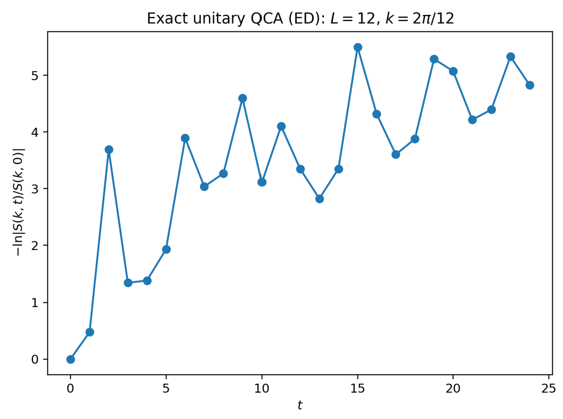
Figure 2.
Exact unitary QCA (ED): diffusion estimates at for .
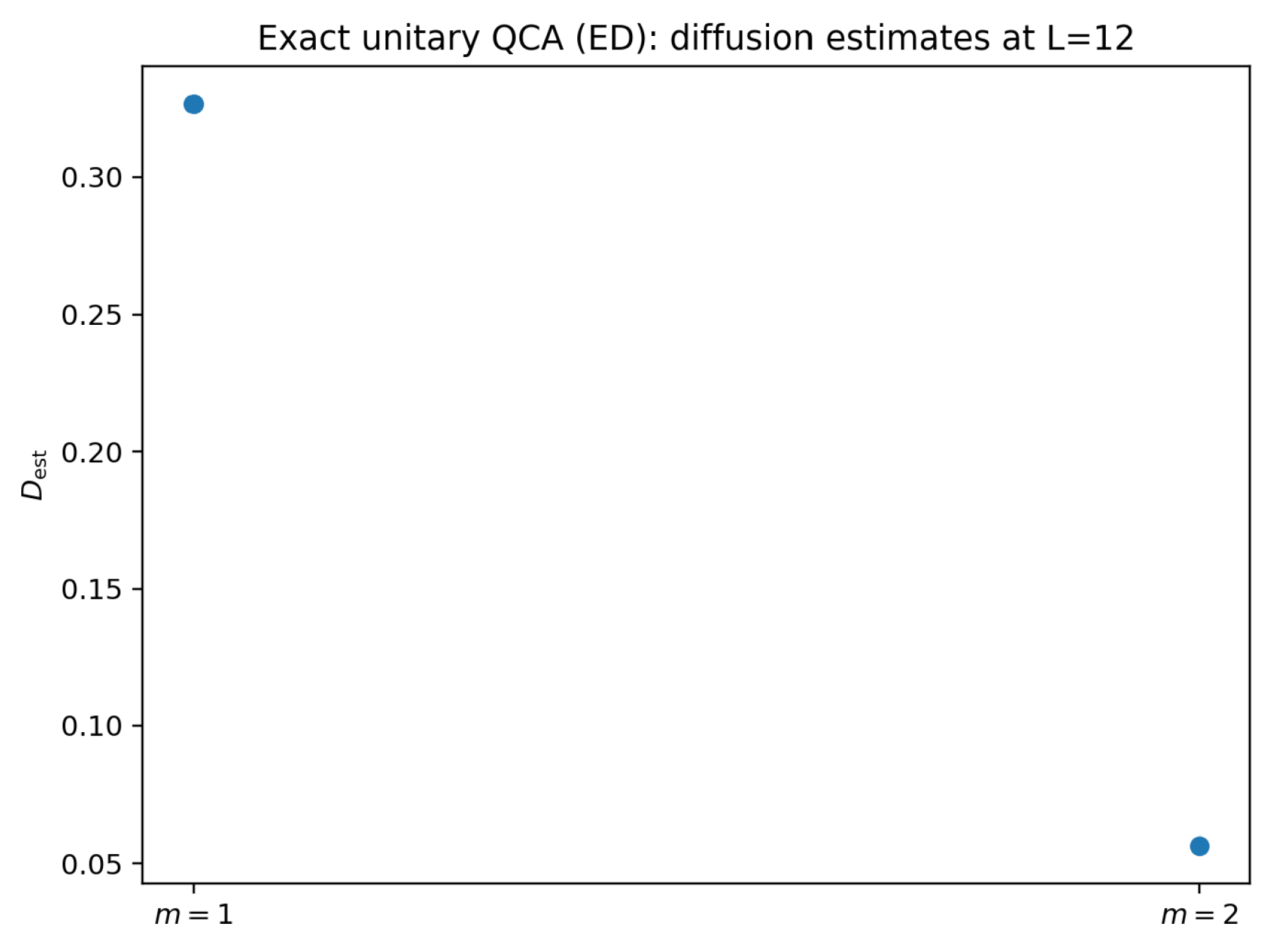
Figure 3.
Supplementary ED cross-check: , (short-time, finite-sample diagnostic).
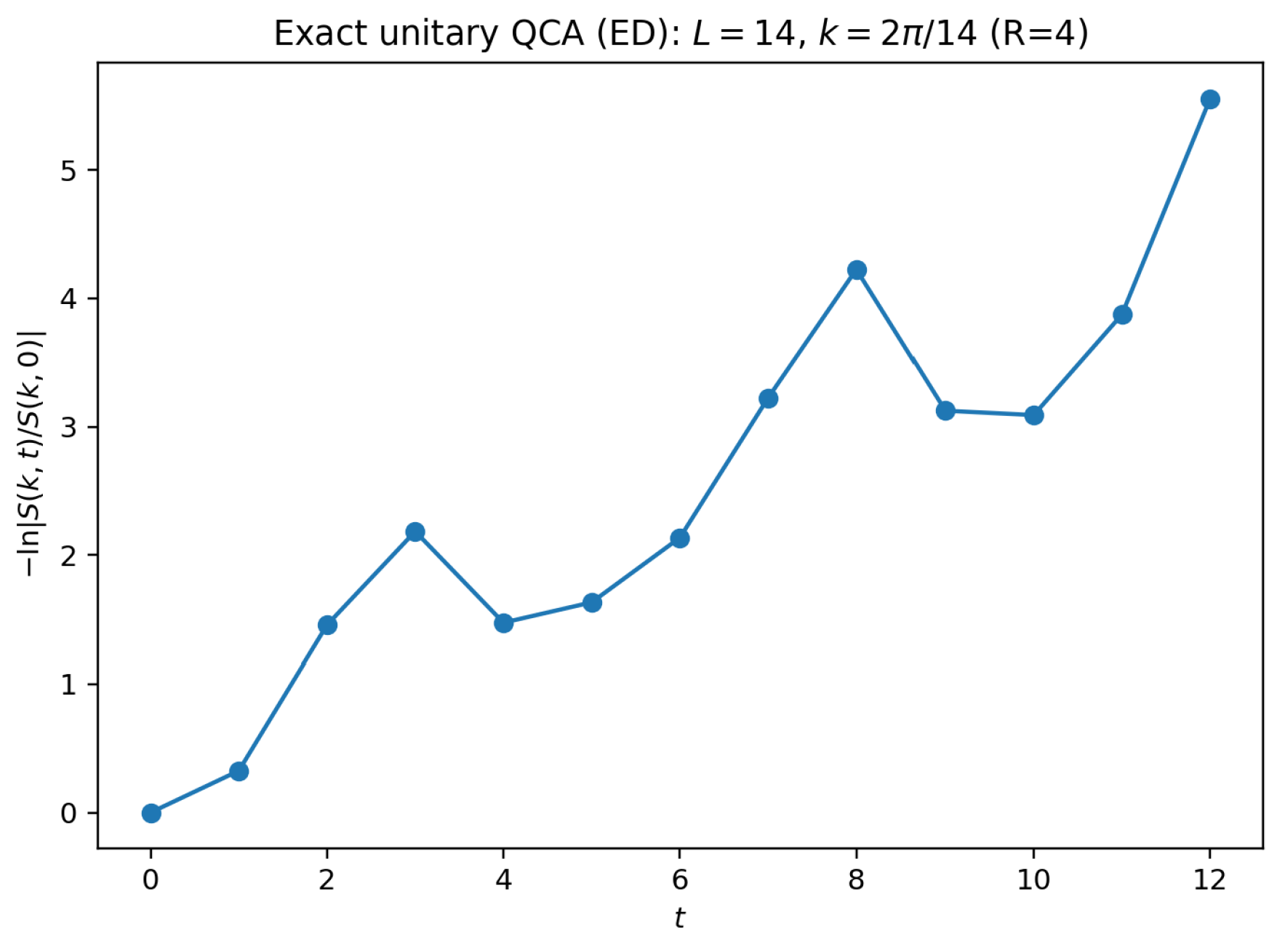
Figure 4.
Moment-channel spectrum (up to ): vs. (diffusion pole).
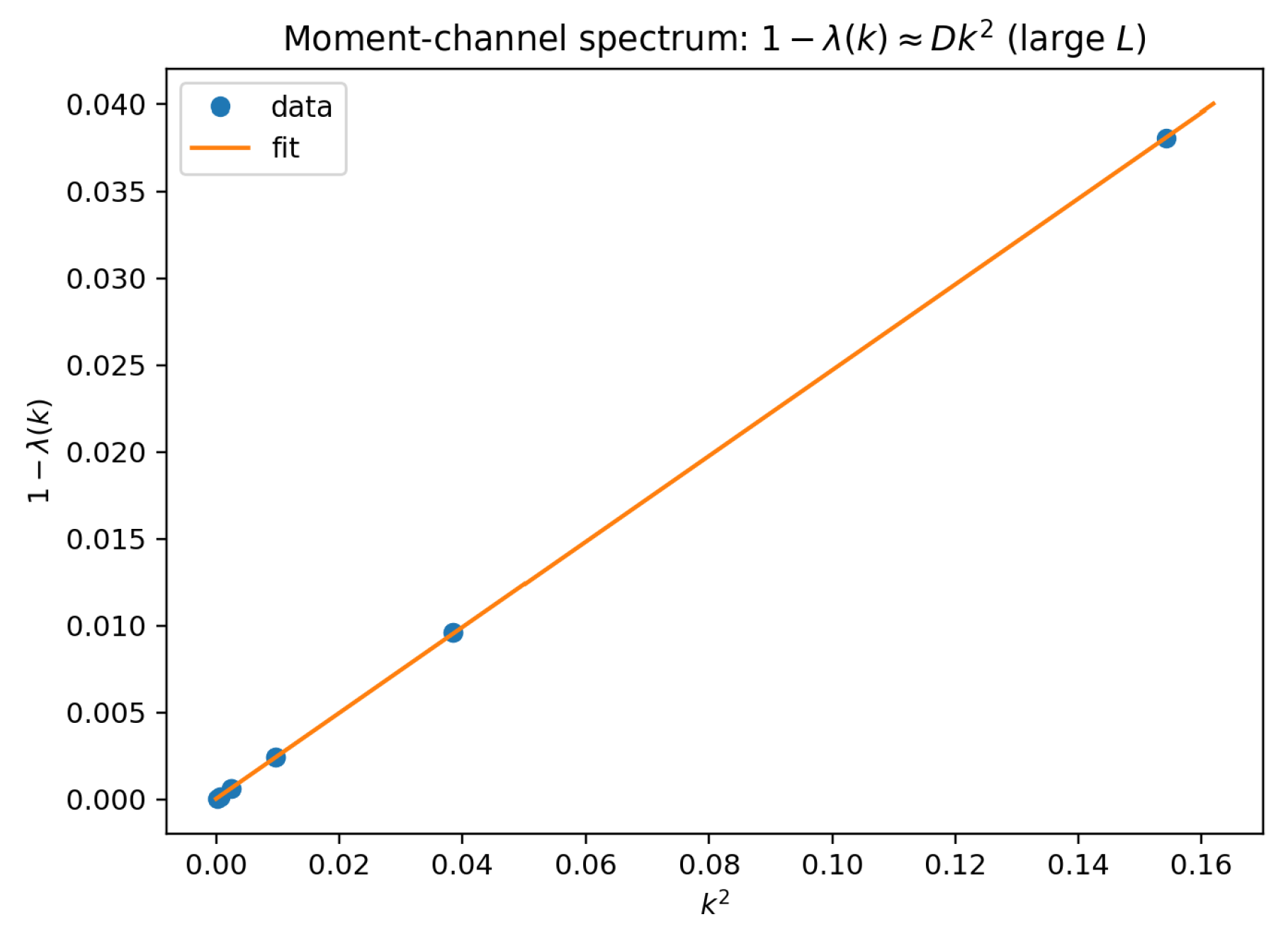
Figure 5.
Moment-channel diffusion: at fixed small k.
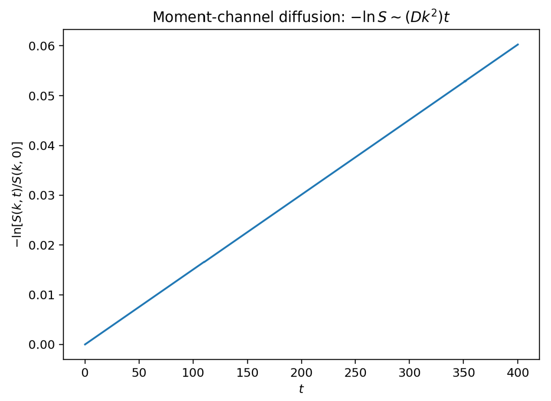
Figure 6.
Moment-channel ballistic/Drude proxy: vs. L (consistent with 0).
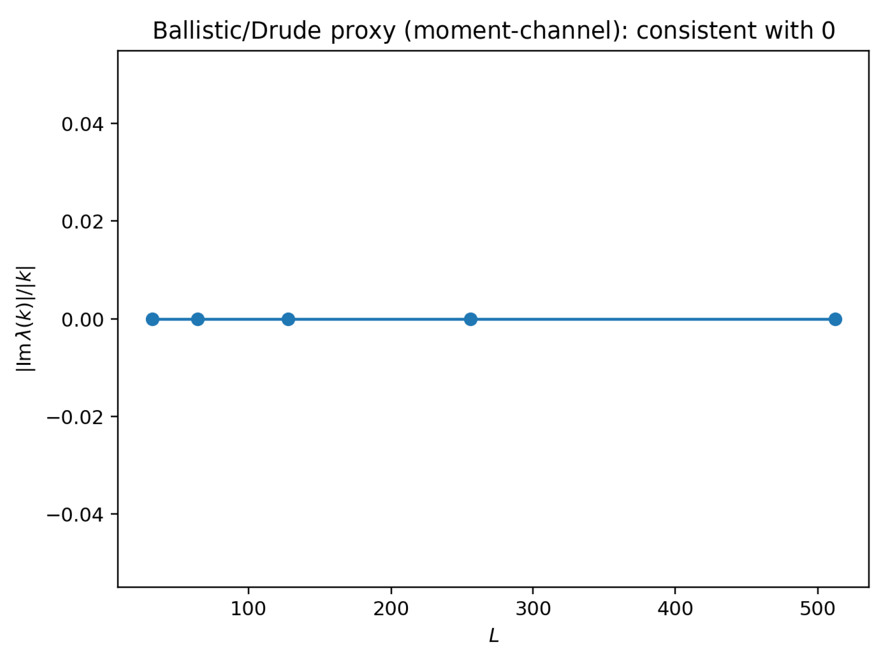
Figure 7.
Unitary QCA TEBD typicality diagnostic (Certified-Numerical): decay proxy at , , . Curves show the MPS bond dimension .
Figure 7.
Unitary QCA TEBD typicality diagnostic (Certified-Numerical): decay proxy at , , . Curves show the MPS bond dimension .
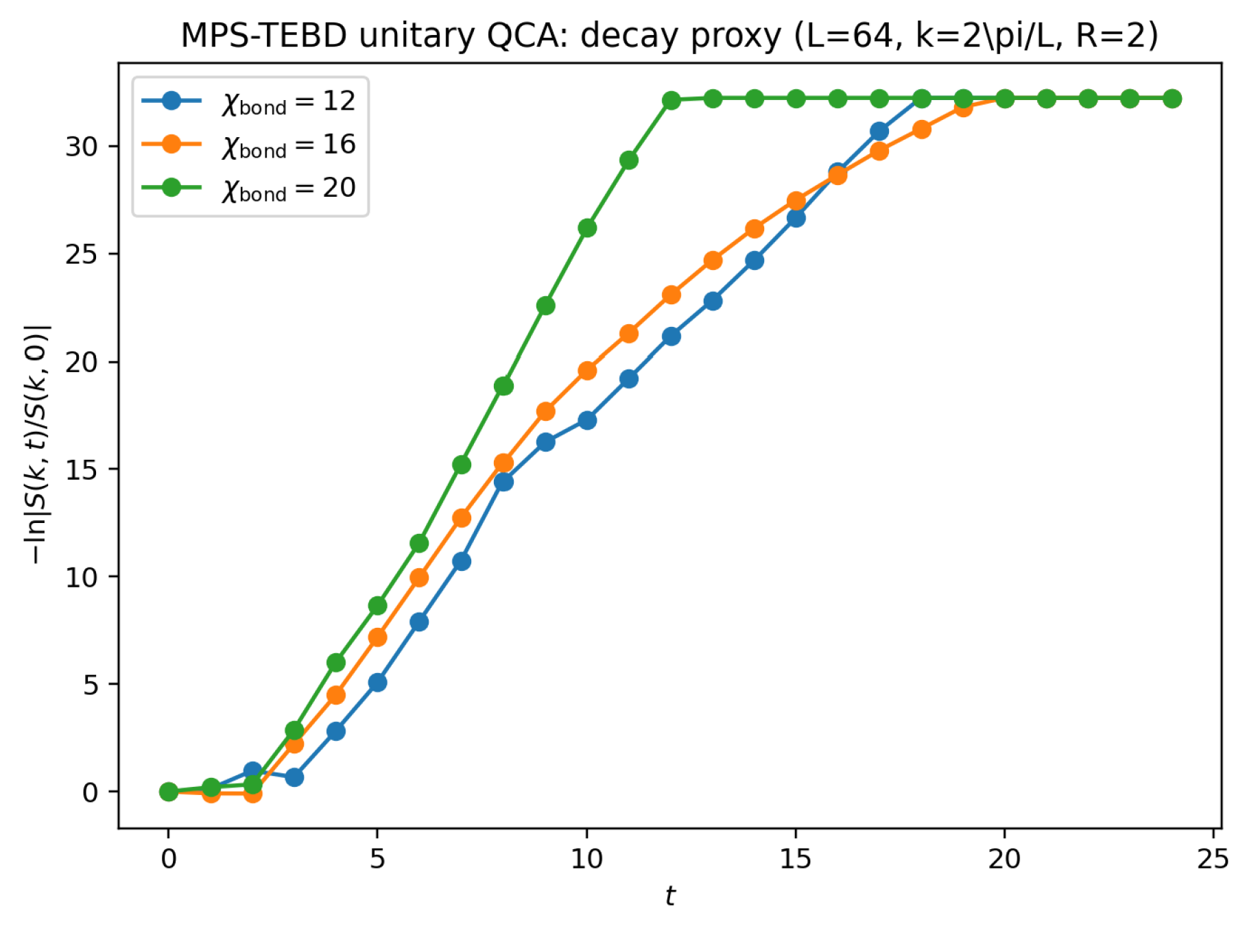
Figure 8.
Unitary QCA TEBD typicality diagnostic (Certified-Numerical): finite-time Drude bound defined in Eq. (22). All runs satisfy the contract threshold and pass the automated PASS/FAIL checks.
Figure 8.
Unitary QCA TEBD typicality diagnostic (Certified-Numerical): finite-time Drude bound defined in Eq. (22). All runs satisfy the contract threshold and pass the automated PASS/FAIL checks.
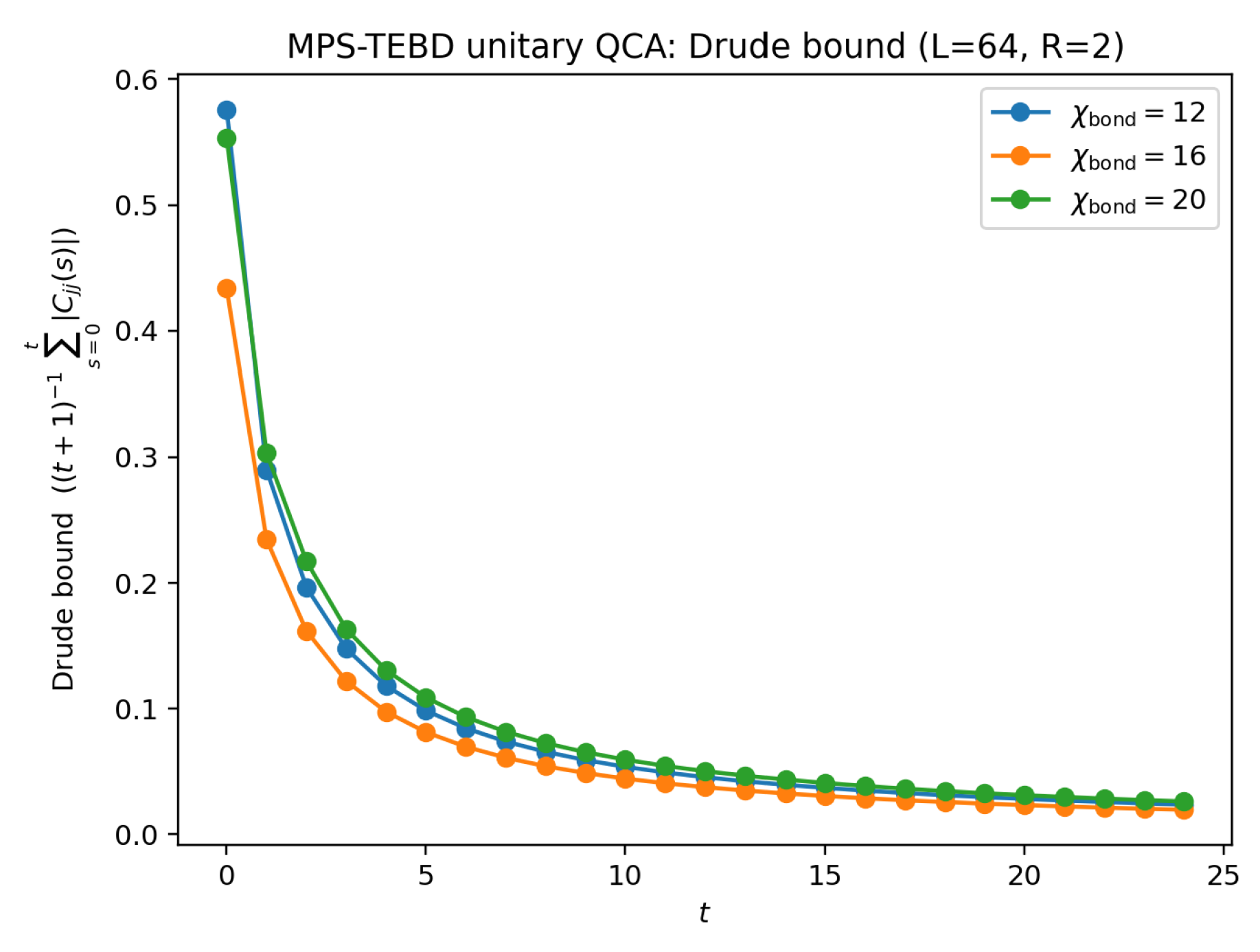
Figure 9.
Convergence diagnostic: extracted vs. for the fixed fit window specified in the contract.
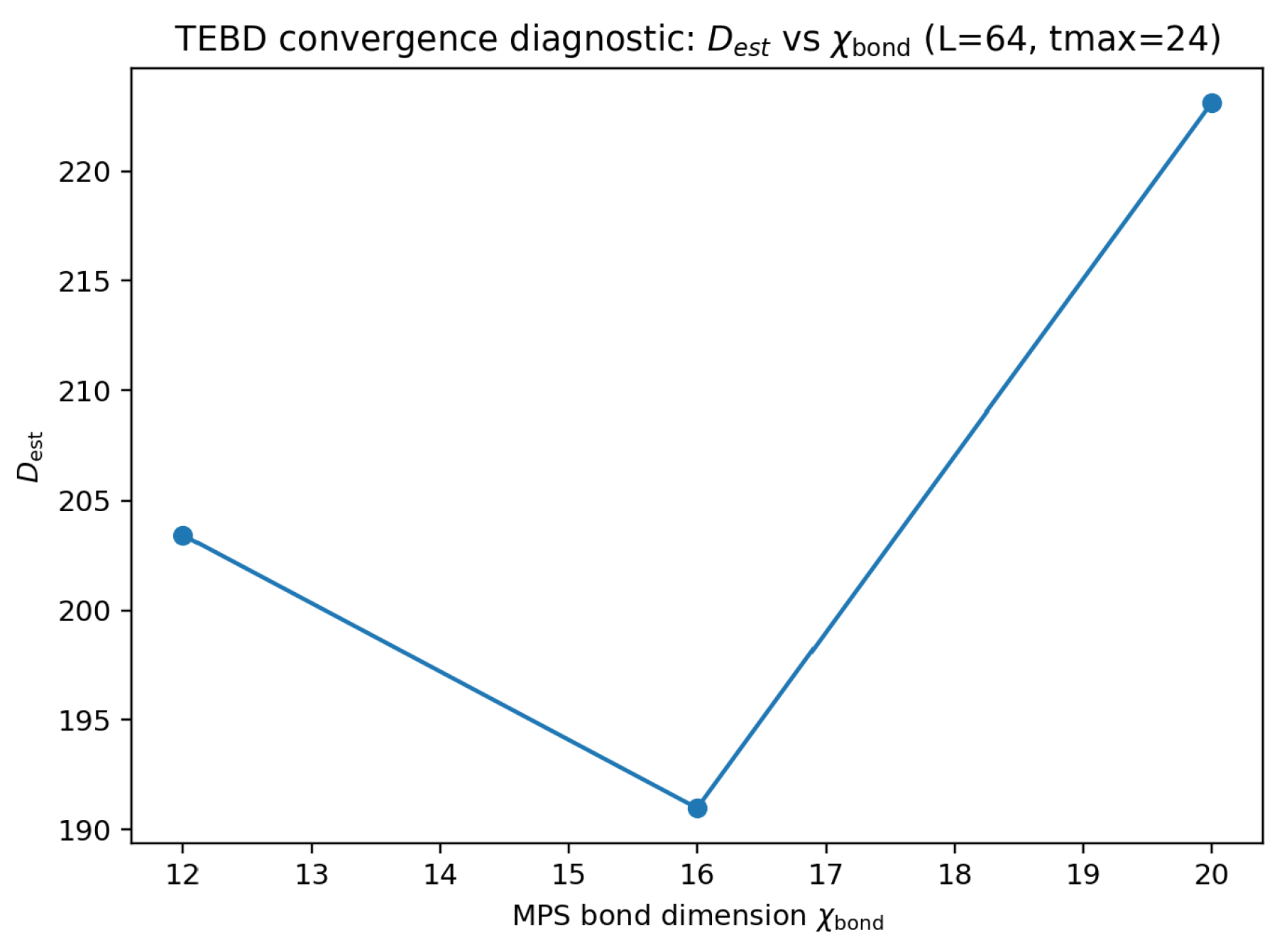
Figure 10.
Benchmark diffusion surface in an Edwards–Wilkinson-type effective model (protocol illustration).
Figure 10.
Benchmark diffusion surface in an Edwards–Wilkinson-type effective model (protocol illustration).
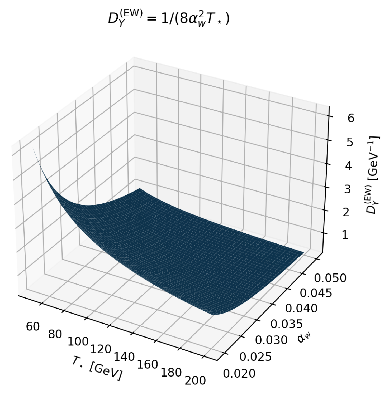
Figure 11.
Benchmark stability surface across regulator/truncation/solver axes (protocol illustration).
Figure 11.
Benchmark stability surface across regulator/truncation/solver axes (protocol illustration).
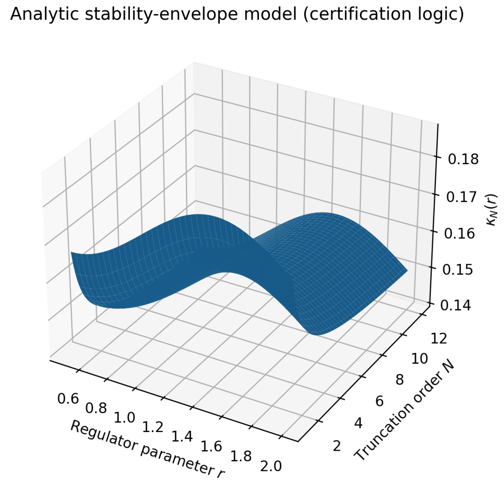
Figure 12.
Benchmark closure surface mapping with fixed and (audited constants).
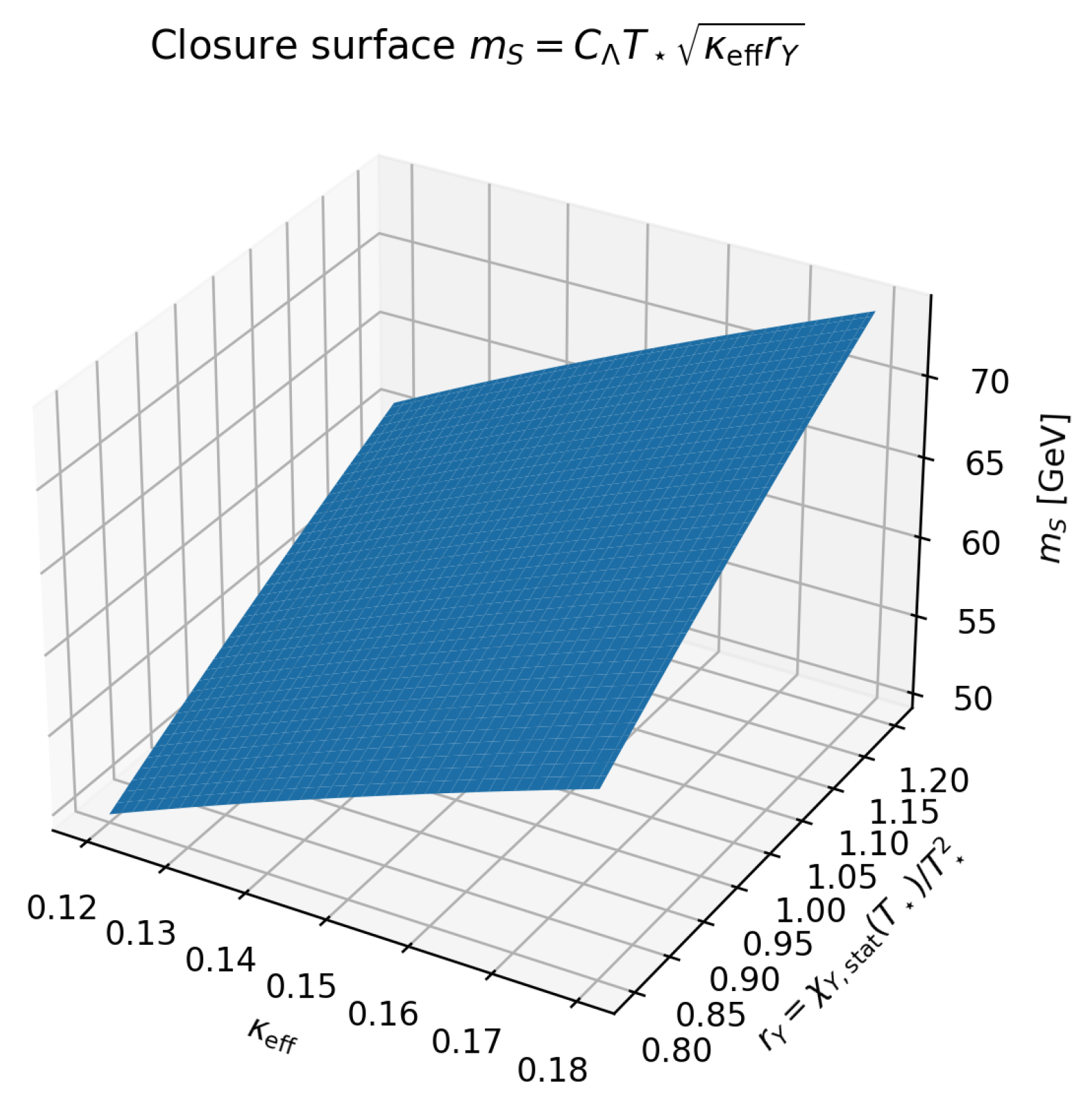
Table 1.
Status labels used throughout.
| Label | Meaning |
|---|---|
| Proven | proved in this manuscript |
| Certified-Numerical | certified numerically under explicit acceptance checks |
| External-Datum | externally supplied interval (non-circular input) |
| Hypothesis | working hypothesis with explicit diagnostics |
| Conjecture | open conjecture stated precisely |
Disclaimer/Publisher’s Note: The statements, opinions and data contained in all publications are solely those of the individual author(s) and contributor(s) and not of MDPI and/or the editor(s). MDPI and/or the editor(s) disclaim responsibility for any injury to people or property resulting from any ideas, methods, instructions or products referred to in the content. |
© 2025 by the authors. Licensee MDPI, Basel, Switzerland. This article is an open access article distributed under the terms and conditions of the Creative Commons Attribution (CC BY) license (http://creativecommons.org/licenses/by/4.0/).
Copyright: This open access article is published under a Creative Commons CC BY 4.0 license, which permit the free download, distribution, and reuse, provided that the author and preprint are cited in any reuse.


