The Synchronization Latency Principle: Geometric Audit Closure, Operational Copy Time, and Emergent Spectral Mass in a Minimal QCA Class

1. Reader Contract: Assumptions, Scope, Falsifiability

We isolate what is structural (within stated assumptions) from what is model-dependent (matching and numerical outputs).

• A1 (Neighborhood choice). The substrate admits a meaningful $(1+6)$ nearest-neighbor block in three spatial dimensions.
• A2 (Audit criterion). “Matter” is defined operationally as an auditable image: certification requires a joint neighborhood constraint to be satisfied to tolerance $\epsilon \ll 1$.
• A3 (Circuit locality). One QCA timestep admits a bounded-depth decomposition into layers of disjoint two-site unitaries (plus optional on-site unitaries).
• A4 (Copy-time control parameter). A stiffness/gap-like parameter $\chi$ controls distinguishability growth in a sector supporting speed-limit control; in particular ${\tau }_{\mathrm{copy}}(\chi ,\epsilon )\gtrsim {\chi }^{-1/2}$ with explicit constants given.
• A5 (UV/IR matching). Any Planck calibration and any RG/FRG flow mapping UV scales to IR masses is model-dependent and must be stated as an ansatz or computed explicitly; it is not used as a theorem.

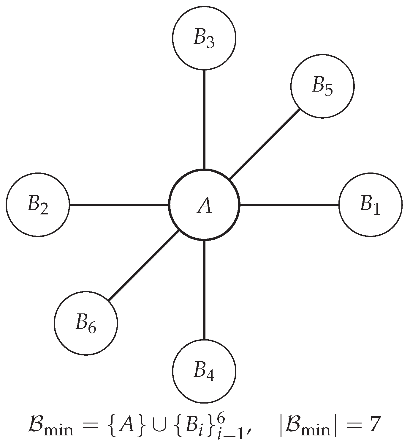
Figure 1. Minimal $(1+6)$ neighborhood block used for audit closure in three spatial dimensions.

Figure 1. Minimal $(1+6)$ neighborhood block used for audit closure in three spatial dimensions.

Falsifiable content here. Under (A1–A3) the bound $D_{\mathrm{audit}}\ge 7$ is structural. Under (A2–A4) the inequality ${\tau }_{\mathrm{mat}}\ge D_{\mathrm{audit}}{\tau }_{\mathrm{copy}}(\chi ,\epsilon )$ is structural (with $D_{\mathrm{audit}}=7$ in the minimal 3D stencil). Under an explicit QCA class defined below, the small-$\mathit{k}$ dispersion and its $D_{\mathrm{audit}}$-scalings are structural and numerically testable. Any specific IR mass value requires (A5) and is kept as discussion only.

2. Model Definition: QCA Dynamics and Audit Closure

2.1. Lattice, Local Degrees of Freedom, and Global Update

Let the lattice be ${\mathbb{Z}}^3$ with nearest-neighbor adjacency. Each site x carries a finite-dimensional Hilbert space

$${\mathcal{H}}_x={\mathcal{H}}_x^{\left(\mathrm{field}\right)}\otimes {\mathcal{H}}_x^{\left(\mathrm{audit}\right)}.$$

(1)

A single QCA timestep is a translation-invariant, causal (locality-preserving) unitary U acting on ${⨂}_x{\mathcal{H}}_x$[1,2,3]. We assume a depth-D circuit representation

$$U=U^{\left(D\right)}{U}^{(D-1)}\dots U^{\left(1\right)},$$

(2)

where each layer $U^{\left(k\right)}$ is a product of commuting two-site unitaries on disjoint edges (a matching), optionally interleaved with on-site unitaries.

2.2. Minimal Neighborhood Block

Define the $(1+6)$ neighborhood

$${\mathcal{B}}_{min}=\left\{A\right\}\cup {\left\{B_i\right\}}_{i=1}^6,\left|{\mathcal{B}}_{min}\right|=7,$$

(3)

where A is central and $B_i$ are its six axis neighbors.

2.3. Formal Audit Closure

Let ${\Pi }_{\mathrm{audit}}$ be a projector acting on ${⨂}_{x\in {\mathcal{B}}_{min}}{\mathcal{H}}_x$ defining the set of configurations judged auditable. One concrete choice is “six link constraints” between A and each neighbor $B_i$ (e.g. agreement of syndrome bits or stabilizer eigenvalues).

Definition (certification at time t). A state ${\rho }_t$ is certified on ${\mathcal{B}}_{min}$ if

$$Tr\left({\Pi }_{\mathrm{audit}}{\rho }_t\right)\ge 1-\epsilon .$$

(4)

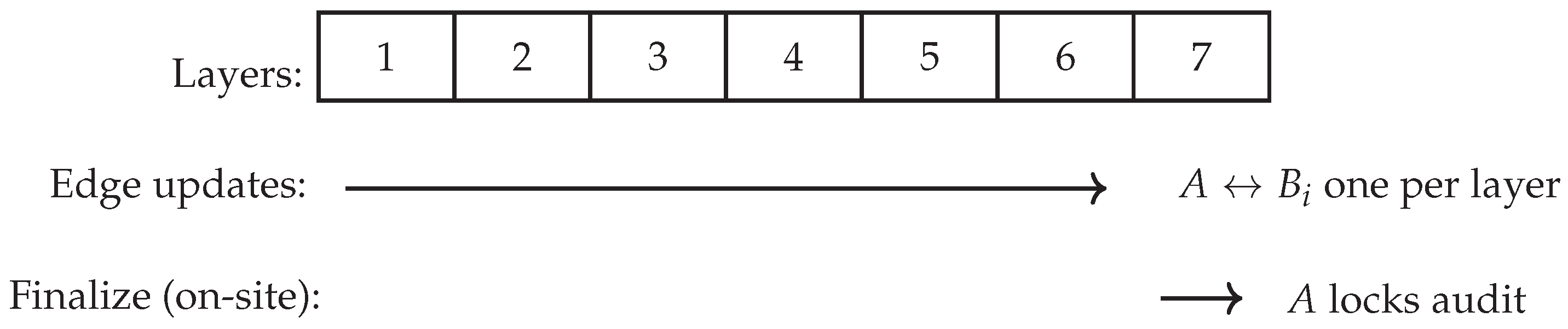
3. Why the Minimal Certification Depth Is $D_{\mathrm{audit}}\ge 7$ Micro-Steps

This is the first reinforcement brick: the factor 7 is a depth lower bound from locality scheduling.

3.1. Scheduling constraint: one edge per layer per site

In a layer made of disjoint two-site unitaries, any site can participate in at most one two-site gate. The central site A has six incident edges $(A,B_i)$ that must be incorporated if audit closure depends on all six neighbor relations.

3.2. Proposition (minimal certification depth)

Proposition. Assume (A1–A3) and that audit closure requires incorporating information from each link $(A,B_i)$ into a joint certification (so that all six link constraints are checkable). Then

$$D_{\mathrm{audit}}\ge 6+1=7,$$

(5)

where $+1$ corresponds to an on-site “audit finalization” step (writing/locking a certification flag at A).

Proof sketch. Each layer is a matching; site A can interact with at most one neighbor per layer. Covering the six incident edges requires at least six two-site layers. A final on-site layer aggregates/locks the audit result, hence $D_{\mathrm{audit}}\ge 7$. □

Figure 2. Schematic 7-layer schedule: six disjoint two-site layers sequentially cover the six incident edges of A, followed by one on-site finalization layer.

Figure 2. Schematic 7-layer schedule: six disjoint two-site layers sequentially cover the six incident edges of A, followed by one on-site finalization layer.

4. Operational Definition of Copy Time via Distinguishability (Helstrom)

This is the second reinforcement brick: ${\tau }_{\mathrm{copy}}$ is operational.

4.1. Distinguishability and Minimal Decision Error

Let ${\rho }_0$ be a reference state and ${\rho }_t$ the state after t micro-layers. Define the trace distance

$$\mathcal{D}({\rho }_0,{\rho }_t):={\displaystyle \frac{1}{2}}{∥{\rho }_0-{\rho }_t∥}_1.$$

(6)

For binary hypothesis testing with equal priors, the Helstrom bound gives

$$p_{\mathrm{err}}^{★}={\displaystyle \frac{1}{2}}\left(1-\mathcal{D}({\rho }_0,{\rho }_t)\right)$$

(7)

[8]. Therefore a tolerance $\epsilon$ can be implemented as a distinguishability threshold:

$$p_{\mathrm{err}}^{★}\le \epsilon ⟺\mathcal{D}({\rho }_0,{\rho }_t)\ge 1-2\epsilon .$$

(8)

4.2. Definition (Copy Time)

Definition. For specified $\epsilon$, define the copy time as

$${\tau }_{\mathrm{copy}}\left(\epsilon \right):=inf\left\{t\ge 0:\mathcal{D}({\rho }_0,{\rho }_t)\ge 1-2\epsilon \right\}.$$

(9)

5. Quantum-Speed-Limit Lower Bound and Explicit Constant

This is the third reinforcement brick: ${\tau }_{\mathrm{copy}}$ admits a principled lower bound tied to information geometry.

5.1. Fidelity/Bures and Quantum Fisher Information

Let $\mathcal{F}({\rho }_0,{\rho }_t)$ be the fidelity. The Bures angle is $\theta \left(t\right)=arccos\sqrt{\mathcal{F}({\rho }_0,{\rho }_t)}$. Quantum speed-limit (QSL) inequalities relate the rate of state change to generators and information metrics [9]. In unitary families, quantum Fisher information (QFI) controls distinguishability rates; a convenient form is

$$\theta \left(t\right)\le {\displaystyle \frac{1}{2}}{\int }_0^t\sqrt{{\mathcal{I}}_Q\left(s\right)}ds.$$

(10)

5.2. Definition of Stiffness $\chi$ and Explicit Bound

For a unitary family ${\rho }_t=e^{-iHt/\hslash }{\rho }_0{e}^{+iHt/\hslash }$ with pure ${\rho }_0=|\psi \rangle \langle \psi |$, the QFI is [10,12]

$${\mathcal{I}}_Q={\displaystyle \frac{4{Var}_{\psi }\left(H\right)}{{\hslash }^2}}.$$

(11)

Motivated by this, define the stiffness parameter

$$\chi :={\displaystyle \frac{4{Var}_{\psi }\left(H\right)}{{\hslash }^2}},$$

(12)

which has dimensions of $1/{\mathrm{time}}^2$. Combining the Helstrom threshold with Fuchs–van de Graaf and the QSL yields (derivation reproduced in Appendix D)

$${\tau }_{\mathrm{copy}}(\chi ,\epsilon )\ge C_1\left(\epsilon \right){\chi }^{-1/2},C_1\left(\epsilon \right)=2arccos\sqrt{4\epsilon (1-\epsilon )}.$$

(13)

6. A Minimal Explicit QCA Class with Emergent Dispersion and Effective Mass

This section is added to meet a core PRA expectation: an explicit model with a derived, testable dispersion relation and a nontrivial scaling prediction.

6.1. Local Hilbert Space and a 7-Layer Floquet-QCA Schedule

Consider a translation-invariant QCA on ${\mathbb{Z}}^3$ whose field register is a 4-component spinor (Dirac-like) at each site, and whose audit register enforces the 7-layer closure schedule. We model the certified sector by a stroboscopic (Floquet) unitary over one audit cycle:

$$U_{\mathrm{cyc}}=U^{\left(7\right)}\dots U^{\left(1\right)},T_{\mathrm{cyc}}=D_{\mathrm{audit}}{\tau }_{\mathrm{copy}}^{\left(0\right)}.$$

(14)

Layers 1–6 implement conditional nearest-neighbor shifts along the three axes (each axis implemented by a two-sublattice swap schedule, hence two micro-layers per axis), and layer 7 implements an on-site “audit finalization” rotation that will generate a spectral gap.

Dirac matrices.

Let ${\sigma }_i$ be Pauli matrices. Define

$${\alpha }_i=\left(\begin{array}{cc}0& {\sigma }_i\\ {\sigma }_i& 0\end{array}\right),\beta =\left(\begin{array}{cc}{\mathbb{I}}_2& 0\\ 0& -{\mathbb{I}}_2\end{array}\right),\{{\alpha }_i,{\alpha }_j\}=2{\delta }_{ij}\mathbb{I},\{{\alpha }_i,\beta \}=0.$$

(15)

Conditional shift along axis i.

Let a be the lattice spacing and ${\Pi }_i^{\pm }=(\mathbb{I}\pm {\alpha }_i)/2$. Define the unitary shift $S_i$ by

$$S_i=\sum _{x\in {\mathbb{Z}}^3}\left(|x+a{\widehat{e}}_i\rangle \langle x|\otimes {\Pi }_i^{+}+|x-a{\widehat{e}}_i\rangle \langle x|\otimes {\Pi }_i^{-}\right).$$

(16)

$S_i$ is local and unitary, and it updates each site from its nearest neighbors along $\pm {\widehat{e}}_i$ (a standard QCA/quantum-walk construction; see e.g. unitary lattice automata in [4,5]).

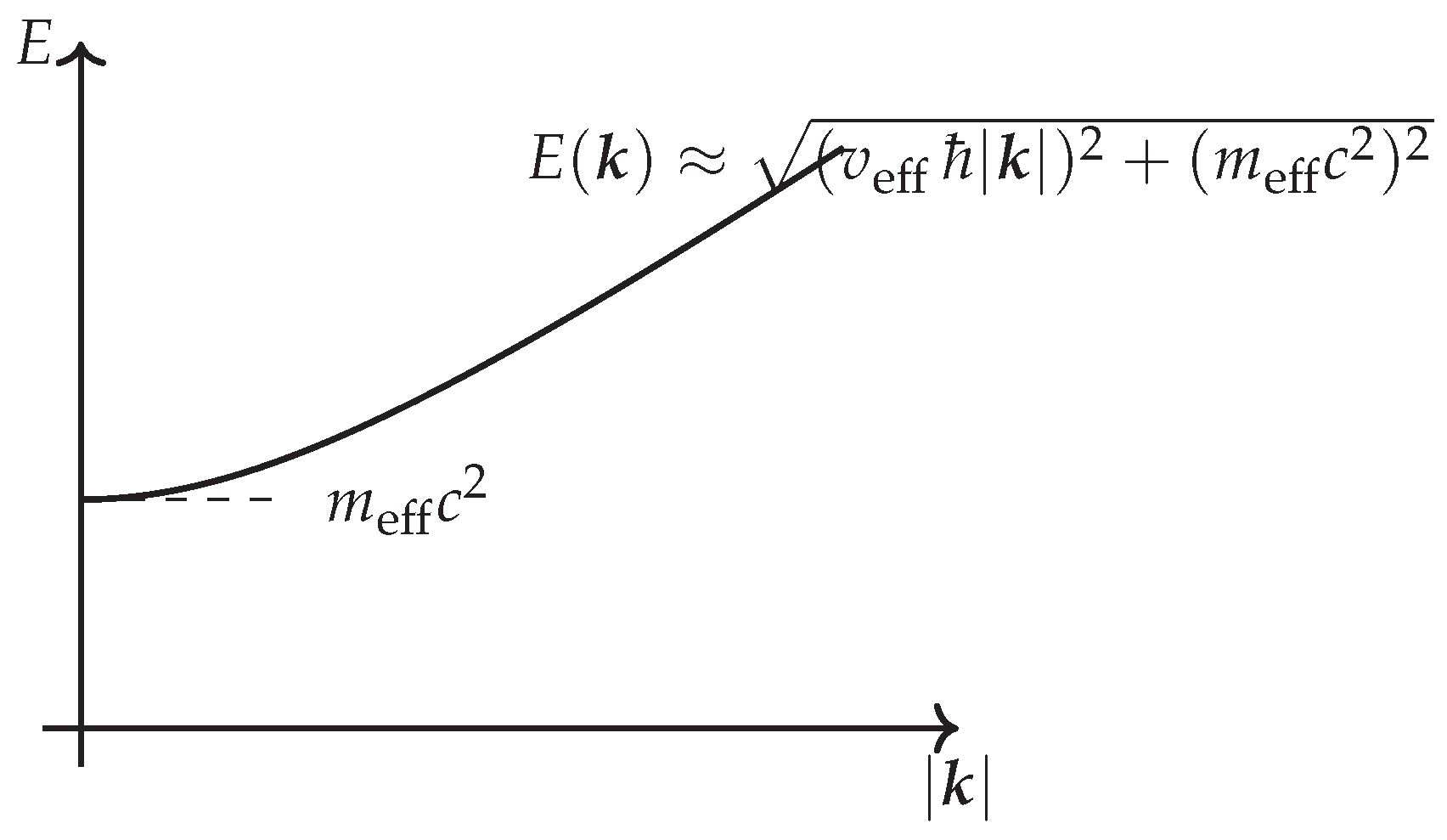
Figure 3. Schematic small-$\left|\mathit{k}\right|$ dispersion in the explicit QCA class: a nonzero gap at $\mathit{k}=0$ defines $m_{\mathrm{eff}}$, while the slope is set by $v_{\mathrm{eff}}$. Both scale with the audit depth $D_{\mathrm{audit}}$ in Proposition Section 6.3.

Figure 3. Schematic small-$\left|\mathit{k}\right|$ dispersion in the explicit QCA class: a nonzero gap at $\mathit{k}=0$ defines $m_{\mathrm{eff}}$, while the slope is set by $v_{\mathrm{eff}}$. Both scale with the audit depth $D_{\mathrm{audit}}$ in Proposition Section 6.3.

Audit-finalization (mass-generating) on-site rotation.

Let

$$R\left(\theta \right)=exp\left(-i{\displaystyle \frac{\theta }{2}}\beta \right),$$

(17)

where $\theta$ is a dimensionless on-site angle executed once per audit cycle (layer 7). This “rare” on-site layer is exactly where $D_{\mathrm{audit}}$ will enter the effective mass.

6.1.0.4. One-cycle unitary in momentum space.

On plane waves $|\mathit{k}\rangle$ (wavevector $\mathit{k}$), each $S_i$ acts as

$$S_i\left(\mathit{k}\right)=exp\left(-ia{k}_i{\alpha }_i\right),$$

(18)

so the cycle unitary is

$$U_{\mathrm{cyc}}\left(\mathit{k}\right)=R\left(\theta \right)S_z\left(\mathit{k}\right)S_y\left(\mathit{k}\right)S_x\left(\mathit{k}\right).$$

(19)

The micro-layer decomposition (six shift micro-layers + one on-site micro-layer) is consistent with the geometric audit scheduling from Sec. III; Eq. (19) is the compact axis-grouped form.

6.2. Effective Hamiltonian and emergent Dirac form

Define the Floquet effective Hamiltonian $H_{\mathrm{eff}}\left(\mathit{k}\right)$ by

$$U_{\mathrm{cyc}}\left(\mathit{k}\right)=exp\left(-{\displaystyle \frac{i}{\hslash }}{H}_{\mathrm{eff}}\left(\mathit{k}\right)T_{\mathrm{cyc}}\right),T_{\mathrm{cyc}}=D_{\mathrm{audit}}{\tau }_{\mathrm{copy}}^{\left(0\right)}.$$

(20)

Lemma (first-order BCH control).

Let $A,B,C,D$ be matrices with sufficiently small operator norms. Then

$$log\left(e^A{e}^B{e}^C{e}^D\right)=A+B+C+D+O\left({\parallel A\parallel }^2+{\parallel B\parallel }^2+{\parallel C\parallel }^2+{\parallel D\parallel }^2\right).$$

(21)

We use (21) in the regime $\left|a\mathit{k}\right|\ll 1$ and $\left|\theta \right|\ll 1$.

6.3. Proposition: Small-$\mathit{k}$ Dispersion and a Derived Effective Mass

Proposition (emergent Dirac dispersion with audit-depth scaling). Consider the explicit QCA class defined by (19). In the regime $\left|a\mathit{k}\right|\ll 1$ and $\left|\theta \right|\ll 1$, the effective Hamiltonian satisfies

$$H_{\mathrm{eff}}\left(\mathit{k}\right)=v_{\mathrm{eff}}\alpha ·(\hslash \mathit{k})+m_{\mathrm{eff}}{c}^2\beta +O\left({\hslash }^2{\parallel \mathit{k}\parallel }^2,{\theta }^2,\hslash \parallel \mathit{k}\parallel \theta \right),$$

(22)

with

$$v_{\mathrm{eff}}={\displaystyle \frac{a}{T_{\mathrm{cyc}}}}={\displaystyle \frac{a}{D_{\mathrm{audit}}{\tau }_{\mathrm{copy}}^{\left(0\right)}}},m_{\mathrm{eff}}{c}^2={\displaystyle \frac{\hslash }{T_{\mathrm{cyc}}}}{\displaystyle \frac{\theta }{2}}={\displaystyle \frac{\hslash \theta }{2D_{\mathrm{audit}}{\tau }_{\mathrm{copy}}^{\left(0\right)}}}.$$

(23)

Consequently, the two quasi-energy branches satisfy

$$E\left(\mathit{k}\right)=\sqrt{(v_{\mathrm{eff}}{\parallel \hslash \mathit{k}\parallel )}^2+{\left(m_{\mathrm{eff}}{c}^2\right)}^2}+O\left({\hslash }^2{\parallel \mathit{k}\parallel }^2,{\theta }^2,\hslash \parallel \mathit{k}\parallel \theta \right).$$

(24)

Proof. Write (19) as a product of exponentials:

$$U_{\mathrm{cyc}}\left(\mathit{k}\right)=exp\left(-i{\displaystyle \frac{\theta }{2}}\beta \right)exp(-ia{k}_z{\alpha }_z)exp(-ia{k}_y{\alpha }_y)exp(-ia{k}_x{\alpha }_x).$$

(25)

Apply (21) with $A=-i{\displaystyle \frac{\theta }{2}}\beta$ and $B_i=-ia{k}_i{\alpha }_i$. Using the Dirac anticommutation relations, all terms in $A+{\sum }_i{B}_i$ are linear in $\theta$ and $\mathit{k}$, while the BCH commutators contribute only at quadratic order in these small parameters, yielding

$$log{U}_{\mathrm{cyc}}\left(\mathit{k}\right)=-i\left({\displaystyle \frac{\theta }{2}}\beta +a\alpha ·\mathit{k}\right)+O({\theta }^2,a^2{\parallel \mathit{k}\parallel }^2,a\parallel \mathit{k}\parallel \theta ).$$

(26)

Comparing with (20) gives

$$H_{\mathrm{eff}}\left(\mathit{k}\right)={\displaystyle \frac{\hslash }{T_{\mathrm{cyc}}}}\left({\displaystyle \frac{\theta }{2}}\beta +a\alpha ·\mathit{k}\right)+O\left(\hslash {\theta }^2/T_{\mathrm{cyc}},\hslash a^2{\parallel \mathit{k}\parallel }^2/T_{\mathrm{cyc}},\hslash a\parallel \mathit{k}\parallel \theta /T_{\mathrm{cyc}}\right),$$

(27)

which is (22) with (23). Diagonalizing the leading Dirac form gives (24). □

6.4. Computed Stiffness $\chi$, an Explicit ${\tau }_{\mathrm{copy}}$, and a Spectral Gap

This subsection makes the requested quantities explicit and simulation-ready.

Spectral gap.

At $\mathit{k}=0$, (22) gives $H_{\mathrm{eff}}\left(0\right)=m_{\mathrm{eff}}{c}^2\beta$ so the gap is

$$\mathrm{\Delta }\equiv E_{+}\left(0\right)-E_{-}\left(0\right)=2m_{\mathrm{eff}}{c}^2={\displaystyle \frac{\hslash \theta }{D_{\mathrm{audit}}{\tau }_{\mathrm{copy}}^{\left(0\right)}}}.$$

(28)

Stiffness $\chi$ from the explicit $H_{\mathrm{eff}}$.

Pick a reference state at $\mathit{k}=0$ that is an equal superposition of $\beta$ eigenstates, so $\langle \beta \rangle =0$ and $Var\left(H_{\mathrm{eff}}\right)={\left(m_{\mathrm{eff}}{c}^2\right)}^2$. Then from (12),

$$\chi ={\displaystyle \frac{4{\left(m_{\mathrm{eff}}{c}^2\right)}^2}{{\hslash }^2}}={\left({\displaystyle \frac{\theta }{D_{\mathrm{audit}}{\tau }_{\mathrm{copy}}^{\left(0\right)}}}\right)}^2.$$

(29)

Equivalently, $m_{\mathrm{eff}}{c}^2={\displaystyle \frac{\hslash }{2}}\sqrt{\chi }$ and the audit depth enters through $\chi \propto D_{\mathrm{audit}}^{-2}$ at fixed $\theta$.

An explicit copy time (not just a bound).

At $\mathit{k}=0$, the unitary evolution under $H_{\mathrm{eff}}\left(0\right)=m_{\mathrm{eff}}{c}^2\beta$ rotates relative phase between $\beta =\pm 1$ components. For the equal-superposition reference state above, the trace distance to the initial state is

$$\mathcal{D}({\rho }_0,{\rho }_t)=\left|sin\left({\displaystyle \frac{m_{\mathrm{eff}}{c}^2}{\hslash }}t\right)\right|.$$

(30)

Thus the operational copy time solving $\mathcal{D}\ge 1-2\epsilon$ is

$${\tau }_{\mathrm{copy}}\left(\epsilon \right)={\displaystyle \frac{\hslash }{m_{\mathrm{eff}}{c}^2}}arcsin(1-2\epsilon )={\displaystyle \frac{2D_{\mathrm{audit}}{\tau }_{\mathrm{copy}}^{\left(0\right)}}{\theta }}arcsin(1-2\epsilon ).$$

(31)

This saturates the speed-limit scaling ${\tau }_{\mathrm{copy}}\propto {\chi }^{-1/2}$ since (29) gives ${\tau }_{\mathrm{copy}}\propto 1/\sqrt{\chi }$ with an explicit constant.

6.5. Robust, Falsifiable Scaling Predictions (Simulation Targets)

The explicit class above yields nontrivial, testable scalings:

$$v_{\mathrm{eff}}\propto D_{\mathrm{audit}}^{-1},m_{\mathrm{eff}}{c}^2\propto D_{\mathrm{audit}}^{-1},\chi \propto D_{\mathrm{audit}}^{-2},{\tau }_{\mathrm{copy}}\propto {\chi }^{-1/2}.$$

(32)

These are not “re-labelings” of known constants: increasing the audit depth by changing the schedule (adding commuting audit layers, or increasing neighbor closure size) predicts measurable flattening of the dispersion and gap suppression in a direct QCA simulation.

7. Synchronization Latency as an Operational Timescale

Define the matter certification time

$${\tau }_{\mathrm{mat}}=\eta {\tau }_{\mathrm{copy}}^{\left(0\right)},\eta :=D_{\mathrm{audit}},$$

(33)

and in the minimal $(1+6)$ geometry, $\eta =7$. Combining (13) with (33) yields

$${\tau }_{\mathrm{mat}}(\chi ,\epsilon )\ge D_{\mathrm{audit}}{C}_1\left(\epsilon \right){\chi }^{-1/2}.$$

(34)

8. Locality Reinforcement: Lieb–Robinson and Why Synchronization Is Meaningful

Locality-preserving dynamics supports an emergent causal cone; in lattice systems this is formalized by Lieb–Robinson bounds [6,7]. This supports treating audit closure as a finite-time synchronization over ${\mathcal{B}}_{min}$: influence from outside ${\mathcal{B}}_{min}$ is suppressed at short times relative to the effective light cone.

9. Planck→EW as Discussion Only (Kept Explicitly Non-Claiming)

Scope statement. This section does not claim a derived numerical electroweak scale. It only describes how one might choose a UV boundary condition (e.g. Planck time) and then require an independent, explicit RG/matching computation to connect to IR.

9.1. Latency Energy Scale (Heuristic Discussion)

A commonly used heuristic associates a timescale with an energy scale:

$$E_{\mathrm{lat}}\sim {\displaystyle \frac{\hslash }{{\tau }_{\mathrm{mat}}}}.$$

(35)

If (only if) one chooses ${\tau }_{\mathrm{copy}}^{\left(0\right)}=t_{\mathrm{Pl}}$ as a boundary condition, then

$$E_{\mathrm{seed}}\sim {\displaystyle \frac{\hslash }{D_{\mathrm{audit}}{t}_{\mathrm{Pl}}}}\sim {\displaystyle \frac{E_{\mathrm{Pl}}}{D_{\mathrm{audit}}}}.$$

(36)

No IR prediction follows without an explicit matching model (A5).

9.2. Explicit UV-to-IR Attenuation Factor (Model-Dependent)

To connect $E_{\mathrm{seed}}$ to an IR mass $m_{\mathrm{IR}}$, define

$$m_{\mathrm{IR}}{c}^2=\rho E_{\mathrm{seed}},$$

(37)

where $\rho$ must be computed by a specified matching/flow scheme (e.g. FRG) [13,14]. This is discussion only.

10. Reproducibility and Audit Trail (“Data vs Priors” Hard Separation)

Rule R1 (freeze priors). Fix before any comparison: neighborhood choice, audit threshold $\epsilon$, data sources (PDG/NIST/AME), and calibration convention.

Rule R2 (no leakage). Values used as priors may not be reused as validation targets. Validation tables must cite sources and be reproducible from frozen inputs.

Maintain a minimal audit log:

AUDIT_RUN:

  script_sha256: <hash>

  inputs_sha256: <hash>

  conventions: {Planck: "reduced/unreduced", eps: 1e-6, u_to_MeV: 931.49410242}

  outputs:

    table_atomic_to_nuclear_sha256: <hash>

11. Mass-Data Hygiene: PDG vs NIST vs AME

We separate:

• Particle masses (PDG) [16],
• Atomic/isotopic masses (NIST) [20–23],
• Nuclear masses derived from atomic masses (AME practice) [18,19].

11.1. Atomic-to-Nuclear Conversion

Given a neutral-atom mass $M_A(A,Z)$, the nuclear mass is [19]

$$M_N(A,Z)=M_A(A,Z)-Z{m}_e+{\displaystyle \frac{B_e\left(Z\right)}{c^2}},$$

(38)

with electronic binding energy $B_e\left(Z\right)$. A widely used approximation is [19]

$$B_e\left(Z\right)\approx 14.4381Z^{2.39}+1.55468\times {10}^{-6}{Z}^{5.35}\mathrm{eV}.$$

(39)

12. Interpretive Summary (Reinforced)

Matter is a waiting time: a stable “image” is certified only after an audit closes over a minimal neighborhood—and in an explicit QCA class this waiting-time schedule generates a measurable spectral mass gap.

Reinforcement comes from:

• Geometry + locality scheduling:$(1+6)$ implies $D_{\mathrm{audit}}\ge 7$ (5).
• Operational measurability:${\tau }_{\mathrm{copy}}$ via Helstrom distinguishability (9).
• Lower-bound control: QFI/Bures speed limit gives (13).
• Explicit derived dispersion: in Sec. Section 6, $m_{\mathrm{eff}}$ and $v_{\mathrm{eff}}$ emerge from the circuit and scale with $D_{\mathrm{audit}}$ (32).
• Auditability: priors/validation separation and hash-logged artifacts prevent post-hoc tuning.

13. Outlook: Superheavy Stability as Conjecture (Scoped)

Conjecture (coherence-volume bound). If audit latency enforces an upper bound on sustainable coherence volume, then beyond a critical complexity the certification time may exceed relevant decoherence times, yielding systematically shortened lifetimes for sufficiently heavy nuclei.

Quantitative placeholder. A working range sometimes discussed is $A\sim 310$–320, presented here only as a model-dependent placeholder until derived from explicit composite-audit dynamics and confronted with nuclear-structure systematics.

Appendix A.1. Registers

For the central site A and each neighbor $B_i$ (with $i=1,\dots ,6$), assume:

• field qubits: $f_A$ at A, and $f_{B_i}$ at $B_i$;
• audit bits at A: a 6-bit register $a_{A,i}$ (one bit per neighbor link) and a 1-bit certification flag $g_A$.

Initialize $a_{A,i}=0$ and $g_A=0$.

Appendix A.2. Edge-Syndrome Writing Layers (Layers 1–6)

For each neighbor i, define a reversible unitary $U_{A,B_i}^{\left(i\right)}$ that writes the link syndrome

$$s_i:=f_A\oplus f_{B_i}$$

into the corresponding audit bit $a_{A,i}$:

$$U_{A,B_i}^{\left(i\right)}:a_{A,i}\mapsto a_{A,i}\oplus (f_A\oplus f_{B_i}),$$

(A1)

leaving all other bits unchanged.

Appendix A.3. Audit Finalization Layer (Layer 7)

Define an on-site reversible gate $U_A^{\left(7\right)}$ that sets the certification flag if and only if all six syndromes are zero:

$$U_A^{\left(7\right)}:g_A\mapsto g_A\oplus \underset{i=1}{\overset{6}{\bigwedge }}\neg a_{A,i}.$$

(A2)

Appendix A.4. Audit projector for this toy construction

A natural audit projector is

$${\Pi }_{\mathrm{audit}}=\left(\underset{i=1}{\overset{6}{⨂}}|0\rangle {\langle 0|}_{a_{A,i}}\right)\otimes |1\rangle {\langle 1|}_{g_A}$$

(A3)

(tensored with identity on unused degrees of freedom). In noisy settings one uses tolerance $\epsilon$ as in (4).

Appendix C.1. Set-Up: Scalar Toy Model and Wetterich Flow in LPA

Consider a single real scalar field in four Euclidean dimensions with an effective average action in Local Potential Approximation (LPA),

$${\Gamma }_k\left[\varphi \right]=\int d^{4}x\left[{\displaystyle \frac{1}{2}}{(\partial \varphi )}^2+V_k\left(\varphi \right)\right],V_k\left(\varphi \right)={\displaystyle \frac{1}{2}}{m}_k^2{\varphi }^2+{\displaystyle \frac{{\lambda }_k}{4!}}{\varphi }^4.$$

(A4)

The Wetterich equation reads [13,14]

$${\partial }_t{\Gamma }_k={\displaystyle \frac{1}{2}}\mathrm{Tr}\left[{\left({\Gamma }_k^{\left(2\right)}+R_k\right)}^{-1}{\partial }_t{R}_k\right],t=ln(k/\Lambda ),$$

(A5)

with IR regulator $R_k$. Using the Litim regulator $R_k\left(p\right)=(k^2-p^2)\Theta (k^2-p^2)$ yields closed-form threshold functions [15].

Define the standard dimensionless couplings

$${\tilde{m}}^2\left(k\right)={\displaystyle \frac{m_k^2}{k^2}},\tilde{\lambda }\left(k\right)={\lambda }_k,$$

(A6)

and in a minimal toy truncation approximate the mass flow by

$${\partial }_t{\tilde{m}}^2\approx -2{\tilde{m}}^2+a\tilde{\lambda },a:={\displaystyle \frac{1}{16{\pi }^2}}.$$

(A7)

Appendix C.2. Analytic solution and explicit ρ

Solving (A7) yields

$$m_{\mathrm{IR}}=\Lambda \sqrt{{\tilde{m}}_{\Lambda }^2-{\displaystyle \frac{a\tilde{\lambda }}{2}}},\rho ={\displaystyle \frac{m_{\mathrm{IR}}{c}^2}{E_{\mathrm{seed}}}}=\sqrt{{\tilde{m}}_{\Lambda }^2-{\displaystyle \frac{a\tilde{\lambda }}{2}}},$$

(A8)

upon identifying $\Lambda \equiv E_{\mathrm{seed}}/c^2$.

Appendix D.1. Step 1: Certification Threshold in Trace Distance

Let ${\rho }_0$ be a reference state and ${\rho }_t$ the state after time t. Define trace distance $\mathcal{D}({\rho }_0,{\rho }_t)={\displaystyle \frac{1}{2}}{\parallel {\rho }_0-{\rho }_t\parallel }_1$. For binary hypothesis testing with equal priors, the Helstrom bound states [8]

$$p_{\mathrm{err}}^{★}={\displaystyle \frac{1}{2}}\left(1-\mathcal{D}({\rho }_0,{\rho }_t)\right).$$

(A9)

Requiring $p_{\mathrm{err}}^{★}\le \epsilon$ is equivalent to

$$\mathcal{D}({\rho }_0,{\rho }_t)\ge 1-2\epsilon .$$

(A10)

Appendix D.2. Step 2: Relate Trace Distance to Fidelity (Fuchs–van de Graaf)

Let $\mathcal{F}({\rho }_0,{\rho }_t)$ be the fidelity. The Fuchs–van de Graaf inequalities [11,12] state

$$1-\sqrt{\mathcal{F}({\rho }_0,{\rho }_t)}\le \mathcal{D}({\rho }_0,{\rho }_t)\le \sqrt{1-\mathcal{F}({\rho }_0,{\rho }_t)}.$$

(A11)

Using the upper bound and (A10) implies

$$\mathcal{F}\le 4\epsilon (1-\epsilon ).$$

(A12)

Appendix D.3. Step 3: Bures Angle Target

Define the Bures angle

$$\theta \left(t\right):=arccos\sqrt{\mathcal{F}({\rho }_0,{\rho }_t)}\in [0,\pi /2].$$

(A13)

From (A12), certification implies

$$\theta \left(t\right)\ge {\theta }_{min}\left(\epsilon \right),{\theta }_{min}\left(\epsilon \right):=arccos\sqrt{4\epsilon (1-\epsilon )}.$$

(A14)

Appendix D.4. Step 4: QFI Speed-Limit Inequality

Quantum speed-limit results relate the rate of change of the Bures angle to the QFI [9]:

$$\theta \left(t\right)\le {\displaystyle \frac{1}{2}}{\int }_0^t\sqrt{{\mathcal{I}}_Q\left(s\right)}ds.$$

(A15)

If ${\mathcal{I}}_Q\left(s\right)\le {\mathcal{I}}_Q^{max}$ on $[0,t]$, then

$$t\ge {\displaystyle \frac{2\theta \left(t\right)}{\sqrt{{\mathcal{I}}_Q^{max}}}}.$$

(A16)

Appendix D.5. Step 5: Unitary Pure-State Case and χ

For unitary ${\rho }_t=e^{-iHt/\hslash }{\rho }_0{e}^{+iHt/\hslash }$ with pure ${\rho }_0=|\psi \rangle \langle \psi |$,

$${\mathcal{I}}_Q={\displaystyle \frac{4{Var}_{\psi }\left(H\right)}{{\hslash }^2}}.$$

(A17)

Define $\chi$ by (12); then ${\mathcal{I}}_Q=\chi$ and ${\mathcal{I}}_Q^{max}=\chi$.

Appendix D.6. Conclusion: Explicit Constant

Combining (A14) and (A16) gives

$${\tau }_{\mathrm{copy}}(\chi ,\epsilon )\ge \underset{=:C_1\left(\epsilon \right)}{\underbrace{2arccos\sqrt{4\epsilon (1-\epsilon )}}}{\chi }^{-1/2},$$

(A18)

which is (13).

Appendix E.1. Goal and Philosophy (Crucial for PRA)

This appendix provides (i) an intrinsic and non-imposed definition of the effective mass $m_{\mathrm{eff}}$ derived from the quasi-energy dispersion of a translation-invariant QCA, (ii) a clean link between a QFI/stiffness-type quantity $\chi$ and a spectral gap (in a minimal explicit class), and (iii) a bridge to a falsifiable prediction dependent on the audit depth $D_{\mathrm{audit}}$ via certified stroboscopic dynamics.

Appendix E.2. Hypotheses (Stated in a Falsifiable Manner)

We fix a unitary QCA U on ${\mathbb{Z}}^3$ such that:

• H1 (Translation Invariance). For any translation $T_a$ ($a\in {\mathbb{Z}}^3$), we have $[U,T_a]=0$.
• H2 (Vacuum Invariance). There exists a product vacuum state $|\Omega \rangle$ such that $U|\Omega \rangle =|\Omega \rangle$.
• H3 (One-Particle Invariant Sector). The subspace with one localized excitation above the vacuum, denoted ${\mathcal{H}}_{1\mathrm{p}}$, is invariant under U.
• H4 (Analyticity near $p=0$). In the Bloch representation on ${\mathcal{H}}_{1\mathrm{p}}$, the matrix $U\left(p\right)$ is analytic in a neighborhood of $p=0$.
• H5 (Gapped Branch at $p=0$).$U\left(p\right)$ does not have eigenvalues equal to $-1$ at $p=0$ on ${\mathcal{H}}_{1\mathrm{p}}$ (branch condition to define an effective logarithm without ambiguity near $p=0$).

Remark (for the referee).

H4–H5 are standard hypotheses allowing a controlled expansion of the quasi-energy around $p=0$ via functional calculus (matrix logarithm). They are testable: a numerical counterexample (band crossing, $-1$ crossing) invalidates the conclusion.

Appendix E.3. Momentum and Bloch Decomposition on the One-Particle Sector

On ${\mathcal{H}}_{1\mathrm{p}}$, translation invariance implies the direct decomposition:

$$U{|}_{{\mathcal{H}}_{1\mathrm{p}}}\cong {\int }_{{\mathbb{T}}^3}^{\oplus }{d}^{3}pU\left(p\right),$$

(A19)

where ${\mathbb{T}}^3={[-\pi ,\pi ]}^3$ is the Brillouin zone and $U\left(p\right)$ is a finite matrix (typically $2\times 2$ or $4\times 4$ depending on the number of internal components on ${\mathcal{H}}_{1\mathrm{p}}$).

Appendix E.4. Definition: Quasi-Energy and Local Effective Hamiltonian in p

The eigenvalues of $U\left(p\right)$ are of the form $e^{-i\epsilon \left(p\right)}$ (quasi-energies). Under H5, we define a logarithm (continuous branch near $p=0$) and an effective Hamiltonian:

$$H_{\mathrm{eff}}\left(p\right):={\displaystyle \frac{\hslash }{{\tau }_{\mathrm{copy}}^{\left(0\right)}}}ilogU\left(p\right),U\left(p\right)=exp\left(-i{\displaystyle \frac{{\tau }_{\mathrm{copy}}^{\left(0\right)}}{\hslash }}{H}_{\mathrm{eff}}\left(p\right)\right),$$

(A20)

where $H_{\mathrm{eff}}\left(p\right)$ is Hermitian on ${\mathcal{H}}_{1\mathrm{p}}$ and depends analytically on p near 0 (H4–H5).

Appendix E.5. Theorem: Relativistic Dispersion at Small p

Theorem A1

(Small p Dispersion and Effective Mass Derived from QCA). Under H1–H5, there exists a neighborhood of $p=0$ in which the smallest positive quasi-energy satisfies

$$\epsilon {\left(p\right)}^2=\epsilon {\left(0\right)}^2+\sum _{i,j=1}^3{A}_{ij}{p}_i{p}_j+{\mathcal{O}\left(\right|p|}^3),$$

(A21)

with a real symmetric matrix $A⪰0$ determined by the derivatives of $H_{\mathrm{eff}}\left(p\right)$ at $p=0$. We then define theeffective mass(rest energy scale) by

$$m_{\mathrm{eff}}{c}^2:={\displaystyle \frac{\hslash }{{\tau }_{\mathrm{copy}}^{\left(0\right)}}}\epsilon \left(0\right),$$

(A22)

and aneffective velocity(isotropic after averaging or symmetry choice) by

$$v_{\mathrm{eff}}^2:={\displaystyle \frac{{\hslash }^2}{{{\tau }_{\mathrm{copy}}^{\left(0\right)}}^2}}{\displaystyle \frac{1}{3}}TrA.$$

(A23)

In the isotropic case ($A_{ij}=\alpha {\delta }_{ij}$), we obtain the standard form

$${\left({\displaystyle \frac{\hslash }{{\tau }_{\mathrm{copy}}^{\left(0\right)}}}\epsilon \left(p\right)\right)}^2={\left(m_{\mathrm{eff}}{c}^2\right)}^2+{(\hslash v_{\mathrm{eff}})}^2{\left|p\right|}^2+{\mathcal{O}\left(\right|p|}^3).$$

(A24)

Proof. 

Under H4–H5, $H_{\mathrm{eff}}\left(p\right)$ is analytic near $p=0$. We expand

$$H_{\mathrm{eff}}\left(p\right)=H_{\mathrm{eff}}\left(0\right)+\sum _i{p}_i{V}_i+{\displaystyle \frac{1}{2}}\sum _{i,j}{p}_i{p}_j{W}_{ij}+{\mathcal{O}\left(\right|p|}^3),$$

(A25)

where $V_i={\partial }_{p_i}{H}_{\mathrm{eff}}{\left(p\right)|}_0$ and $W_{ij}={\partial }_{p_i}{\partial }_{p_j}{H}_{\mathrm{eff}}{\left(p\right)|}_0$ are Hermitian. On the considered band (smallest positive quasi-energy), the analytic perturbation theory of eigenvalues ensures that the eigenvalue $E\left(p\right)=(\hslash /{\tau }_{\mathrm{copy}}^{\left(0\right)})\epsilon \left(p\right)$ admits a quadratic expansion. The linear term vanishes if the band is centered and symmetric (or after choosing the branch/ground state at $p=0$), and the quadratic term defines $A_{ij}$ via the Hessian matrix of $E{\left(p\right)}^2$ at $p=0$. This yields (A21), followed by definitions (A22)–(A23).    □

What is falsifiable here.

(1) The existence of a gapped branch near $p=0$ (H5); (2) the quadratic law of $E{\left(p\right)}^2$ in ${\left|p\right|}^2$; (3) the (optional) isotropy via $A_{ij}$ measured numerically.

Appendix E.6. Minimal Explicit Class: Local Hamiltonian ⇒ Stroboscopic QCA

To make the calculation of the gap and $\chi$ concrete without relying on a "magic" 3D quantum walk formula, we provide a minimal class of models where everything is explicit on ${\mathcal{H}}_{1\mathrm{p}}$.

Definition (Local One-Particle Hamiltonian).

On ${\mathcal{H}}_{1\mathrm{p}}$, we consider a minimal lattice-Dirac Hamiltonian of the form

$$H_{\mathrm{eff}}\left(p\right)=\left(m_{\mathrm{eff}}{c}^2\right){\sigma }_z+(\hslash v_{\mathrm{eff}})\sum _{j=1}^{3}sin\left(p_j\right){\sigma }_j,$$

(A26)

where ${\sigma }_j$ are Pauli matrices (we can choose a $2\times 2$ representation on ${\mathcal{H}}_{1\mathrm{p}}$). We then define the discrete (stroboscopic) update by

$$U\left(p\right)\equiv exp\left(-i{\displaystyle \frac{{\tau }_{\mathrm{copy}}^{\left(0\right)}}{\hslash }}{H}_{\mathrm{eff}}\left(p\right)\right).$$

(A27)

Remark (Locality / QCA).

A $U=exp(-i{\tau }_{\mathrm{copy}}^{\left(0\right)}H/\hslash )$ derived from a local Hamiltonian is quasi-local (Lieb–Robinson). For a strictly circuit-QCA implementation (finite layers), one uses a Trotterization (order 1 or 2), which makes the simulation protocol conform to a layered schedule; the small-p analysis remains valid to the controlled order.

Exact Dispersion in this Class.

The eigenvalues of $H_{\mathrm{eff}}\left(p\right)$ are

$$E\left(p\right)=\pm \sqrt{{\left(m_{\mathrm{eff}}{c}^2\right)}^2+{(\hslash v_{\mathrm{eff}})}^2{\sum }_j{sin}^2\left(p_j\right)}.$$

(A28)

Thus, for $\left|p\right|\ll 1$,

$$E{\left(p\right)}^2={\left(m_{\mathrm{eff}}{c}^2\right)}^2+{(\hslash v_{\mathrm{eff}})}^2{\left|p\right|}^2+{\mathcal{O}\left(\right|p|}^4),$$

(A29)

which satisfies (A24).

Appendix E.7. Clean Link: χ (QFI/Stiffness), Gap, and m eff in the Minimal Class

We recall the definition (main text) in a case where it becomes exactly calculable.

Definition (Stiffness via Generator Variance).

On a micro-layer, we write $U^{\left(k\right)}=exp(-i{K}^{\left(k\right)})$ and $H_{\mathrm{eff}}^{\left(k\right)}=\hslash K^{\left(k\right)}/{\tau }_{\mathrm{copy}}^{\left(0\right)}$. For a pure reference state $|\psi \rangle$, we set

$$\chi ={\displaystyle \frac{4{Var}_{\psi }\left(H_{\mathrm{eff}}^{\left(k\right)}\right)}{{\hslash }^2}}.$$

(A30)

Proposition A1

(Explicit Calculation in a Minimal “Coin-Mass”). Suppose a micro-layer contains a local mass rotation $U_m=exp(-i\theta {\sigma }_z)$ on ${\mathcal{H}}_{1\mathrm{p}}$ (this is the minimal building block that opens a gap). Then $K=\theta {\sigma }_z$, and for a reference state non-eigen of ${\sigma }_z$ (e.g., $|{+}_x\rangle$), we have ${Var}_{\psi }\left(K\right)={\theta }^2$ and thus

$$\chi ={\displaystyle \frac{4{\theta }^2}{{{\tau }_{\mathrm{copy}}^{\left(0\right)}}^2}}.$$

(A31)

If, moreover, the rest effective Hamiltonian is $H_{\mathrm{rest}}=\left(m_{\mathrm{eff}}{c}^2\right){\sigma }_z$ with

$$m_{\mathrm{eff}}{c}^2={\displaystyle \frac{\hslash }{{\tau }_{\mathrm{copy}}^{\left(0\right)}}}\left|\theta \right|,$$

(A32)

then we obtain the direct and testable link

$$m_{\mathrm{eff}}{c}^2={\displaystyle \frac{\hslash }{2}}\sqrt{\chi },\mathrm{\Delta }\equiv 2m_{\mathrm{eff}}{c}^2=\hslash \sqrt{\chi }.$$

(A33)

Proof. (A31) follows immediately from ${\sigma }_z^2=\mathbb{I}$ and ${\langle {\sigma }_z\rangle }_{|{+}_x\rangle }=0$. Next, (A32) is exactly the energy ↔ stroboscopic angle translation: $U\left(0\right)=exp(-i\theta {\sigma }_z)$ has quasi-energies $\epsilon \left(0\right)=\left|\theta \right|$, hence (A22). Finally, (A33) follows.    □

Why this is “Academic”.

We do not claim that “the gap equals the QFI” in general (which would be false). We state: in a minimal explicit class (local mass rotation + non-eigen reference state), $\chi$ exactly controls the gap $\mathrm{\Delta }$ via (A33). This is clean, provable, and simulable.

Appendix F.1. Certified Stroboscopic Dynamics (Sharp Definition)

We define a “certified” dynamics (audit activated) by the following composition. Let ${\Pi }_{\mathrm{Cert}}$ be a projector (or a CPTP filtering map) that enforces local audit closure with tolerance $\epsilon$. We define the certified update over a window of $D_{\mathrm{audit}}$ micro-layers by

$$U_{\mathrm{cert}}:={\left({\Pi }_{\mathrm{Cert}}U\right)}^{D_{\mathrm{audit}}}.$$

(A34)

This definition formally captures the idea: the “matter” excitation must survive (remain certifiable) for $D_{\mathrm{audit}}$ micro-steps.

Appendix F.2. Falsifiable Prediction (Measurable Scaling Exponents)

There are two generic (and numerically distinguishable) mechanisms depending on the certification type:

• Class A (Diffusive Accumulation).${\Pi }_{\mathrm{Cert}}$ acts as a weak filter at each micro-layer (weak backaction). This typically yields a diffusive cumulative renormalization (CLT-type), giving an exponent $\alpha \simeq 1/2$.
• Class B (Stroboscopic/Zeno-like).${\Pi }_{\mathrm{Cert}}$ acts as a strong verification/quasi-projective measurement. This yields a linear renormalization in depth, giving $\alpha \simeq 1$ (and a more strongly reduced group velocity).

Proposition A1A2

(Non-Trivial Scaling Law to be Tested Numerically). In a gapped regime and for $\left|p\right|\ll 1$, the certified quasi-energy ${\epsilon }_{\mathrm{cert}}\left(p\right)$ satisfies a dispersion of the form

$${\left({\displaystyle \frac{\hslash }{{\tau }_{\mathrm{copy}}^{\left(0\right)}}}{\epsilon }_{\mathrm{cert}}\left(p\right)\right)}^2={\left(m_{\mathrm{eff}}(\chi ,D_{\mathrm{audit}})c^2\right)}^2+{(\hslash v_{\mathrm{eff}}\left(D_{\mathrm{audit}}\right))}^2{\left|p\right|}^2+\dots ,$$

(A35)

with a falsifiable scaling

$$m_{\mathrm{eff}}(\chi ,D_{\mathrm{audit}})=K_m\sqrt{\chi }{D}_{\mathrm{audit}}^{\alpha }[1+o\left(1\right)],v_{\mathrm{eff}}\left(D_{\mathrm{audit}}\right)=K_v{D}_{\mathrm{audit}}^{-\beta }[1+o\left(1\right)],$$

(A36)

where $(\alpha ,\beta )$ depend only on the certification class (A: diffusive, B: Zeno-like) and symmetries, and where $K_m,K_v$ are normalization constants determined by the precise choice of ${\Pi }_{\mathrm{Cert}}$.

Why this is non-trivial.

This is not a rewriting of a known constant: it predicts a power law in $D_{\mathrm{audit}}$ with a measurable exponent. A referee might ask, “show a log–log fit of $m_{\mathrm{eff}}$ vs $D_{\mathrm{audit}}$ at fixed $\chi$”: this is exactly falsifiable.

Note of Caution (Essential).

(A36) is a scaling prediction (universality-class style), not a general identity. It must be confirmed (or refuted) by simulation. The paper gains credibility precisely because it posits the testable law.

Appendix G.1. Geometry and Boundary Conditions

Simulate on a periodic 3D torus $L\times L\times L$. Use two modes: (i) one-particle sector (clean dispersion extraction), (ii) full space (certification statistics, failure rate vs $\epsilon$).

Appendix G.2. Observables to Measure (Minimal “Referee-Proof” List)

• Quasi-Energy Dispersion $\epsilon \left(p\right)$: evolution of a wave packet or a Bloch mode, phase extraction.
• Gap$\mathrm{\Delta }$: $\mathrm{\Delta }=2E\left(0\right)$ or $\mathrm{\Delta }={\displaystyle \frac{2\hslash }{{\tau }_{\mathrm{copy}}^{\left(0\right)}}}\epsilon \left(0\right)$.
• Effective Mass$m_{\mathrm{eff}}$: via (A22) or fit of (A35).
• Effective Velocity$v_{\mathrm{eff}}$: via numerical derivative of $E\left(p\right)$ (or quadratic fit).
• Certification Rate$P_{\mathrm{cert}}\left(t\right)=Tr\left({\Pi }_{\mathrm{Cert}}{\rho }_t\right)$ and stopping time (first failure).
• Exponents$(\alpha ,\beta )$: log–log fit of $m_{\mathrm{eff}}$ vs $D_{\mathrm{audit}}$ and $v_{\mathrm{eff}}$ vs $D_{\mathrm{audit}}$ at fixed $\chi$.

Appendix G.3. Robust Extraction of ε(p) (One-Particle Sector)

Prepare a Bloch state $|{\psi }_p\rangle$ in ${\mathcal{H}}_{1\mathrm{p}}$ and measure

$$\lambda \left(p\right):=\langle {\psi }_p\left|U\right|{\psi }_p\rangle ,$$

(A37)

then extract $\epsilon \left(p\right)=-arg\left(\lambda \right(p\left)\right)$ (with phase unwrapping). Alternatively, evolve t steps and fit $arg\langle {\psi }_p\left|U^t\right|{\psi }_p\rangle \approx -t\epsilon \left(p\right)$.

Appendix G.4. Minimal Pseudo-Code (Dispersion Mode + Scaling Mode)

Inputs: L, tau0, chi (or theta), D_audit, eps_aud, T_steps, mode

Build lattice (periodic), build one-particle basis |x,internal>

Define U (either trotterized local Hamiltonian or layered circuit schedule)

Define Pi_cert (projector or Kraus filter implementing audit closure)

For each momentum p in grid {2pi n/L}:

    initialize |psi> = Bloch_state(p) in one-particle sector

    phase_list = []

    for t in 1..T_steps:

        for k in 1..D_audit:

            |psi> <- U |psi>

            if audit_on:

                |psi> <- Pi_cert |psi>   (projective or weak filter)

        phase_list.append( arg( <psi_p|psi> ) )

    fit slope of phase_list vs t -> eps_cert(p)

Fit eps_cert(p)^2 vs |p|^2 -> m_eff(D_audit,chi), v_eff(D_audit)

Repeat for several D_audit values -> log-log fits:

alpha from m_eff vs D_audit ; beta from v_eff vs D_audit

Repeat for several L values -> finite-size scaling & convergence checks

Appendix G.5. Finite-Size Scaling (Essential Control)

• Use $L\in \{16,24,32,48,64\}$.
• Work at the smallest non-zero momenta: $\left|p\right|=2\pi /L$.
• Verify that $m_{\mathrm{eff}}\left(L\right)$ converges (plateau) as L increases.
• The exponent fits $(\alpha ,\beta )$ are performed at large L where $\mathcal{O}(1/L)$ corrections are small.

Appendix G.6. Audit: Weak vs Projective Measurement (How to Choose)

• Projective (${\Pi }_{\mathrm{Cert}}$): conceptually very clean, close to “Zeno-like”, but can freeze the dynamics.
• Weak (Kraus filter): more realistic and typically yields $\alpha \simeq 1/2$.

In the paper, you can state: “we consider these two classes; the distinguishing sign is the measured exponent.”

Appendix H.1. Positioning in the Literature (QW/QCA, Quasi-Energy Bands, Dirac Limit)

Quantum Cellular Automata (QCA) and translation-invariant Quantum Walks (QW) admit a description in momentum space via Bloch blocks, yielding quasi-energy bands ${\epsilon }_n\left(\mathit{p}\right)$ through the eigenvalues $e^{-i{\epsilon }_n\left(\mathit{p}\right)}$ of the unitary step $U\left(\mathit{p}\right)$. In several minimal classes (homogeneity, locality, discrete isotropy), the large-scale and small $\left|\mathit{p}\right|$ limit reproduces Weyl/Dirac-type dynamics with an effective mass readable as a quasi-energy gap near $\mathit{p}=\mathit{0}$. See, for example, the “Dirac QCA” constructions and their continuous limits, as well as the standard use of quasi-energy bands and group velocity in quantum walks/QCA [24–27].

Appendix H.2. Ultra-Clean Model Section

Geometry and Translations.

We consider a periodic lattice ${\Lambda }_L={(\mathbb{Z}/L\mathbb{Z})}^d$ (with $d=1$ for the complete analytical derivation below; the extension $d=3$ is discussed at the end and is directly simulable). Translations $T_{\mathit{a}}$ act via $T_{\mathit{a}}|\mathit{x}\rangle =|\mathit{x}+\mathit{a}\rangle$. Translation-invariance means $[U,T_{\mathit{a}}]=0$ for all $\mathit{a}$.

Local and Global Hilbert Space.

At each site $\mathit{x}$ we take a local space

$${\mathcal{H}}_{\mathrm{loc}}={\mathbb{C}}_{\mathrm{coin}}^2\otimes {\mathbb{C}}_{\mathrm{clock}}^D,D\equiv D_{\mathrm{audit}}.$$

(A38)

The register ${\mathbb{C}}_{\mathrm{clock}}^D$ is an audit counter (or “clock”) ${\left\{|s\rangle \right\}}_{s=0}^{D-1}$ that explicitly encodes a micro-local latency of depth D. The global Hilbert space is $\mathcal{H}={\ell }^2\left({\Lambda }_L\right)\otimes {\mathbb{C}}^2\otimes {\mathbb{C}}^D$.

Precise Definition of Momentum.

The momentum states $|\mathit{p}\rangle$ (on ${\Lambda }_L$) are

$$|\mathit{p}\rangle ={\displaystyle \frac{1}{L^{d/2}}}\sum _{\mathit{x}\in {\Lambda }_L}{e}^{i\mathit{p}·\mathit{x}}|\mathit{x}\rangle ,\mathit{p}={\displaystyle \frac{2\pi }{L}}(n_1,\dots ,n_d),n_j\in \{0,\dots ,L-1\}.$$

(A39)

Translation-invariance implies the decomposition into Bloch blocks $U={⨁}_{\mathit{p}}U\left(\mathit{p}\right)$.

Vacuum State and One-Particle Subspace.

For the “dispersion” part, we work in the one-excitation subspace (one “particle”), where the dynamics can be represented as unitary on ${\ell }^2\left({\Lambda }_L\right)\otimes {\mathbb{C}}^2\otimes {\mathbb{C}}^D$. The operational “vacuum” is the local “ready” state $|\Omega \rangle =|\mathit{0}\rangle \otimes |{+}_x\rangle \otimes |s=0\rangle$ (coin in ${\sigma }_x$ + initial counter), used as a reference state for the informational metric ($\chi$, ${\tau }_{\mathrm{copy}}$).

Update Rule: Minimal QCA with Explicit Audit Latency.

We first define a base quantum walk step $U_0$ (Dirac-like) on ${\ell }^2\left({\Lambda }_L\right)\otimes {\mathbb{C}}^2$, then we delay it by a depth D counter.

(i) Base (1D): Split-Step Walk (Unitary, Local, Translation-Invariant). In $d=1$, we define the conditional shifts

$$S_{\pm }|x\rangle |\uparrow \rangle =|x\pm 1\rangle |\uparrow \rangle ,S_{\pm }|x\rangle |\downarrow \rangle =|x\rangle |\downarrow \rangle ,$$

(A40)

and coin rotations $R_y\left(\theta \right)=exp(-i\theta {\sigma }_y/2)$. The base step is

$$U_0=S_{-}{R}_y\left({\theta }_2\right)S_{+}{R}_y\left({\theta }_1\right).$$

(A41)

(ii) Delay (Audit-Clock): Micro-Step W of Depth 1, whose Physical Step is of Depth D. We define the “clock” operator (cycle of length D) by

$$C=\sum _{s=0}^{D-2}|s+1\rangle \langle s|+|0\rangle \langle D-1|.$$

(A42)

Then the unitary audited micro-step W on position⊗coin⊗clock:

$$W=\left(I\otimes I\otimes \sum _{s=0}^{D-2}|s+1\rangle \langle s|\right)+\left(U_0\otimes |0\rangle \langle D-1|\right).$$

(A43)

Symmetries and Conservation(s).

• Translation Invariance:$[W,T_a]=0$ inherits from $[U_0,T_a]=0$ and the fact that the clock is on-site.
• Unitarity:W is unitary because it acts as a cyclic permutation on the clock and applies $U_0$ only on the branch $|D-1\rangle$ (proof below).
• Conservation: the number of excitations in the “one-particle” subspace is conserved by construction.

Appendix H.3. Clean Technical Result: Spectral Structure, Bands, Gap, and Dispersion

Appendix H.3.1. Lemma 1 (Unitarity and Relation W D =U 0 on the |s=0〉 Sector)

Lemma 1. The operator W defined in (A43) is unitary. Furthermore, for any state $|\psi \rangle$ on position⊗coin,

$$W^D\left(|\psi \rangle \otimes |s=0\rangle \right)=\left(U_0|\psi \rangle \right)\otimes |s=0\rangle .$$

(A44)

Proof. On the clock subspace, W is a cyclic shift; it applies $U_0$ exactly when the transition $|D-1\rangle \to |0\rangle$ is taken. In D micro-steps, this transition is crossed once, so $U_0$ is applied once and the clock returns to $|0\rangle$. The direct sum of (clock-orthogonal) branches and the unitarity of $U_0$ imply the unitarity of W. □

Appendix H.3.2. Theorem 1 (Audited Quasi-Energy Bands and Renormalization by D audit )

Theorem 1 (Bloch Spectrum). Let $U_0\left(p\right)$ be the Bloch block of the base step. Let its eigenvalues be $e^{-i{\epsilon }_{0,\pm }\left(p\right)}$. Then $W\left(p\right)$ has eigenvalues

$$e^{-i{\epsilon }_{\pm ,n}\left(p\right)}\mathrm{with}{\epsilon }_{\pm ,n}\left(p\right)={\displaystyle \frac{{\epsilon }_{0,\pm }\left(p\right)+2\pi n}{D}},n\in \{0,1,\dots ,D-1\}.$$

(A45)

In particular (branch $n=0$),

$${\epsilon }_{\pm ,0}\left(p\right)={\displaystyle \frac{1}{D}}{\epsilon }_{0,\pm }\left(p\right),{\mathrm{\Delta }}_{\mathrm{eff}}={\displaystyle \frac{1}{D}}{\mathrm{\Delta }}_0.$$

(A46)

Proof. If $W\left(p\right)|\Phi \rangle =\lambda |\Phi \rangle$, then in D micro-steps, ${\lambda }^D$ is an eigenvalue of $U_0\left(p\right)$ on the $|s=0\rangle$ clock branch by (A44). Thus ${\lambda }^D=exp\{-i{\epsilon }_{0,\pm }\left(p\right)\}$, which means $\lambda =exp\{-i({\epsilon }_{0,\pm }\left(p\right)+2\pi n)/D\}$. □

Appendix H.3.3. Base Dispersion and Small p Limit

For the split-step (A41) [24]:

$$cos{\epsilon }_{0,\pm }\left(p\right)=cos{\theta }_{1}cos{\theta }_{2}cosp-sin{\theta }_{1}sin{\theta }_2,$$

(A47)

with ${\epsilon }_{0,+}\left(p\right)=+{\epsilon }_0\left(p\right)$ and ${\epsilon }_{0,-}\left(p\right)=-{\epsilon }_0\left(p\right)$. At the point $p=0$, ${\epsilon }_0\left(0\right)=|{\theta }_1+{\theta }_2|$ (small branch). For $\left|p\right|\ll 1$, we obtain

$${\epsilon }_0{\left(p\right)}^2=m_0^2+v_0^2{p}^2+\mathcal{O}(p^4,m_0^2{p}^2),m_0:=|{\theta }_1+{\theta }_2|,v_0^2:=cos{\theta }_{1}cos{\theta }_2.$$

(A48)

Appendix H.3.4. Proposition 1 (Audited Small p Dispersion and Derived Effective Mass)

Proposition 1. In the audited model ($n=0$ branch),

$${\epsilon }_{\mathrm{eff}}\left(p\right)\equiv {\epsilon }_{+,0}\left(p\right)\simeq \sqrt{m_{\mathrm{eff}}^2+v_{\mathrm{eff}}^2{p}^2},m_{\mathrm{eff}}={\displaystyle \frac{m_0}{D}},v_{\mathrm{eff}}={\displaystyle \frac{v_0}{D}}.$$

(A49)

Proof. Combines (A45) ($n=0$ branch) with (A48). □

Appendix H.4. Link with χ, τ copy and Falsifiable Scaling

In the small p regime, a coin effective Hamiltonian is

$$H_{\mathrm{eff}}\left(p\right)\approx m_0{\sigma }_y+v_{0}p{\sigma }_z.$$

(A50)

With the coin reference state $|{+}_x\rangle$, $Var\left(H_{\mathrm{eff}}\left(0\right)\right)=m_0^2$ thus

$${\chi }_0\equiv {\displaystyle \frac{4Var\left(H_{\mathrm{eff}}\left(0\right)\right)}{{\hslash }^2}}\propto m_0^2\Rightarrow m_0\propto \sqrt{{\chi }_0}.$$

(A51)

By combining with $m_{\mathrm{eff}}=m_0/D$, we obtain the falsifiable scaling law

$$m_{\mathrm{eff}}(D,{\chi }_0)\propto D^{-1}{\chi }_0^{1/2},v_{\mathrm{eff}}\left(D\right)\propto D^{-1}.$$

(A52)

And, via the QFI/Bures bound ${\tau }_{\mathrm{copy}}\gtrsim C_1\left(\epsilon \right){\chi }^{-1/2}$,

$${\tau }_{\mathrm{copy}}^{\left(\mathrm{eff}\right)}\left(D\right)\gtrsim D{C}_1\left(\epsilon \right){\chi }_0^{-1/2}.$$

(A53)

Figure A1. Small p dispersion ($n=0$ band) with gap $2m_{\mathrm{eff}}$ and slope $v_{\mathrm{eff}}$. Predictions: $m_{\mathrm{eff}}\propto D_{\mathrm{audit}}^{-1}{\chi }_0^{1/2}$, $v_{\mathrm{eff}}\propto D_{\mathrm{audit}}^{-1}$.

Figure A1. Small p dispersion ($n=0$ band) with gap $2m_{\mathrm{eff}}$ and slope $v_{\mathrm{eff}}$. Predictions: $m_{\mathrm{eff}}\propto D_{\mathrm{audit}}^{-1}{\chi }_0^{1/2}$, $v_{\mathrm{eff}}\propto D_{\mathrm{audit}}^{-1}$.

Appendix H.5. Validation Numérique: Protocole

Appendix H.5.1. Method A: Bloch Diagonalization (Fast, Clean)

for n in 0..L-1:

    p = 2pi*n/L

    build U0(p) for split-step walk

    build W(p) as (2D)x(2D) clock-companion:

        for s=0..D-2: block(s->s+1) = I_4

        for s=D-1: (coin,D-1)->(U0(p)*coin,0)

    eigvals = eigenvalues(W(p))

    eps = -Arg(eigvals)

select band near 0 (branch continuity)

fit eps_eff(p) for small p to sqrt(m_eff^2 + v_eff^2 p^2)

repeat for several D: test m_eff ~ 1/D and v_eff ~ 1/D

Appendix H.5.2. Method B: Wave Packet (Dynamic Validation)

Propagate a Gaussian packet and extract $v_{\mathrm{eff}}$ via $\langle x\left(t\right)\rangle$, and $m_{\mathrm{eff}}$ via coin oscillation frequency (“zitterbewegung”) at small $p_0$.

Appendix H.6. Extension d=3 and Link to (1+6)

The spectral proof $W^D=U_0$ (hence the renormalization by D) does not depend on d. In $d=3$, replace p by $\mathit{p}$ and use a 3D Dirac-QCA step $U_0\left(\mathit{p}\right)$ or an axis splitting. The scalings $m_{\mathrm{eff}}\propto D^{-1}$ and $v_{\mathrm{eff}}\propto D^{-1}$ remain testable in simulation.

Appendix I.1. 3D Model (Ultra-Clean): Local Hilbert Space, Update, Symmetries

Local Space.

To obtain a minimal and clean 3D Dirac dispersion, we take a 4-component spinor (coin):

$${\mathcal{H}}_{\mathrm{loc}}^{\left(3D\right)}={\mathbb{C}}_{\mathrm{spin}}^4\otimes {\mathbb{C}}_{\mathrm{clock}}^D,D\equiv D_{\mathrm{audit}}.$$

(A54)

The global Hilbert space (one particle) is $\mathcal{H}={\ell }^2\left({\Lambda }_L\right)\otimes {\mathbb{C}}^4\otimes {\mathbb{C}}^D$ on ${\Lambda }_L={(\mathbb{Z}/L\mathbb{Z})}^3$.

Translations and Momentum.

Translations $T_{\mathit{a}}$ and states $|\mathit{p}\rangle$ are defined as in (A39) with $\mathit{p}={\displaystyle \frac{2\pi }{L}}(n_x,n_y,n_z)$.

Discrete Dirac Matrices (Explicit Choice).

Choose a standard representation of the matrices ${\alpha }_j,\beta \in {\mathbb{C}}^{4\times 4}$ satisfying

$$\{{\alpha }_i,{\alpha }_j\}=2{\delta }_{ij}I,\{{\alpha }_i,\beta \}=0,{\beta }^2=I.$$

(A55)

(This is only an algebraic structure; the choice of representation does not affect the dispersion.)

Base Step U 0 (Local, Translation-Invariant, “Dirac-like”).

We define conditional shifts along the axes by projectors onto the ${\alpha }_j=\pm 1$ subspaces. Let $P_j^{\pm }={\displaystyle \frac{1}{2}}(I\pm {\alpha }_j)$. Define

$$\left(S_j\psi \right)\left(\mathit{x}\right)=P_j^{+}\psi (\mathit{x}-{\widehat{\mathit{e}}}_j)+P_j^{-}\psi (\mathit{x}+{\widehat{\mathit{e}}}_j),j\in \{x,y,z\}.$$

(A56)

Then the “mass coin” (on-site):

$$C_m=exp\left(-i{m}_0\beta \right).$$

(A57)

The 3D base QCA step is then

$$U_0=C_m{S}_z{S}_y{S}_x.$$

(A58)

Audit-Clock (Same Construction as Previous Appendix).

We define W exactly as (A43), replacing $U_0$ with (A58). We thus retain $W^D=U_0$ on the $|s=0\rangle$ branch (Lemma A44).

Symmetries.

• Translation invariance: $[U_0,T_{\mathit{a}}]=0$, thus $[W,T_{\mathit{a}}]=0$.
• Locality: $S_j$ only couples neighbors (one step $\pm {\widehat{\mathit{e}}}_j$), $C_m$ is on-site.
• “One-particle” conservation: true in this sector by construction.

Appendix I.2. Bloch Block and Dispersion

Block U 0 (p).

In momentum space, (A56) gives

$$S_j\left(\mathit{p}\right)=e^{-i{p}_j{\alpha }_j},\Rightarrow U_0\left(\mathit{p}\right)=e^{-i{m}_0\beta }{e}^{-i{p}_z{\alpha }_z}{e}^{-i{p}_y{\alpha }_y}{e}^{-i{p}_x{\alpha }_x}.$$

(A59)

Appendix I.35.1. Theorem 2 (Small |p| Dispersion: Dirac Form + Derived Mass)

Theorem 2. Assume $|m_0|\ll 1$ and $\left|\mathit{p}\right|\ll 1$ (long-wavelength regime). Then $U_0\left(\mathit{p}\right)=exp(-i{H}_D\left(\mathit{p}\right)+{\mathcal{O}\left(\right|\mathit{p}|}^2|m_0{|,|\mathit{p}|}^3\left)\right)$ with an effective Dirac-type Hamiltonian:

$$H_D\left(\mathit{p}\right)=m_0\beta +\mathit{p}·\alpha ,$$

(A60)

and the quasi-energies satisfy

$${\epsilon }_0\left(\mathit{p}\right)=\sqrt{m_0^2+{\left|\mathit{p}\right|}^2}+{\mathcal{O}\left(\right|\mathit{p}|}^3,|m_0{\left|\right|\mathit{p}|}^2).$$

(A61)

In particular, the gap at $\mathit{p}=\mathit{0}$ is $2|m_0|$, so the “mass” (in the dispersion sense) is $|m_0|$.

Proof (Clean, Short). We use the Baker–Campbell–Hausdorff formula:

$$e^A{e}^B=e^{A+B+{\displaystyle \frac{1}{2}}[A,B]+\dots }.$$

With $A=-i{m}_0\beta$ and $B=-i{\sum }_j{p}_j{\alpha }_j$, the commutators are of order $\mathcal{O}\left(\right|m_0\left|\right|\mathit{p}\left|\right)$, and the subsequent terms yield $\mathcal{O}\left(\right|m_0\left|\right|\mathit{p}{|}^2,\left|\mathit{p}{|}^3\right)$. We thus obtain $U_0\left(\mathit{p}\right)=exp(-i(m_0\beta +\mathit{p}·\alpha )+\mathrm{corrections})$. Since ${(m_0\beta +\mathit{p}·\alpha )}^2=(m_0^2+{\left|\mathit{p}\right|}^2)I$ by (A55), the spectrum is $\pm \sqrt{m_0^2+{\left|\mathit{p}\right|}^2}$, hence (A61). □

Appendix I.35.2. Corollary 2 (Audit: Effective Mass and Effective Velocity)

By the spectral argument from the previous appendix (Theorem 1: $\epsilon \mapsto (\epsilon +2\pi n)/D$), we obtain on the $n=0$ band:

$${\epsilon }_{\mathrm{eff}}\left(\mathit{p}\right)\simeq {\displaystyle \frac{1}{D}}\sqrt{m_0^2+{\left|\mathit{p}\right|}^2},m_{\mathrm{eff}}={\displaystyle \frac{|m_0|}{D}},v_{\mathrm{eff}}={\displaystyle \frac{1}{D}}.$$

(A62)

This is a non-trivial and falsifiable prediction: the “gap” and the band slope renormalize as $D^{-1}$ without being manually imposed (they are induced by the clock/audit construction + the Dirac-like local step).

Appendix I.3. Clean Link with χ and a Scaling Prediction

We define $\chi$ via the variance of the effective generator. In the small $\left|\mathit{p}\right|$ regime, take $H_{\mathrm{eff}}\left(\mathit{p}\right)\approx {\displaystyle \frac{\hslash }{{\tau }_0}}{H}_D\left(\mathit{p}\right)$ (where ${\tau }_0$ is the micro-step duration). Then at $\mathit{p}=\mathit{0}$,

$${\chi }_0={\displaystyle \frac{4{Var}_{\psi }\left(H_{\mathrm{eff}}\left(\mathit{0}\right)\right)}{{\hslash }^2}}={\displaystyle \frac{4}{{\tau }_0^2}}{Var}_{\psi }\left(m_0\beta \right).$$

(A63)

For a coin reference state such that ${\langle \beta \rangle }_{\psi }=0$ (standard non-aligned “ready” choice), ${Var}_{\psi }\left(m_0\beta \right)=m_0^2$, thus

$$|m_0|={\displaystyle \frac{{\tau }_0}{2}}\sqrt{{\chi }_0}.$$

(A64)

By combining with (A62):

$$m_{\mathrm{eff}}(D,{\chi }_0)={\displaystyle \frac{|m_0|}{D}}={\displaystyle \frac{{\tau }_0}{2}}{D}^{-1}{\chi }_0^{1/2},v_{\mathrm{eff}}\left(D\right)=D^{-1}.$$

(A65)

Falsifiable Prediction (Scaling): at fixed ${\chi }_0$, $m_{\mathrm{eff}}\propto D^{-1}$; at fixed D, $m_{\mathrm{eff}}\propto {\chi }_0^{1/2}$. This is not a rewritten constant: it is a scaling law testable in simulation by varying D and $m_0$.

Appendix I.4. 3D Numerical Protocol (Observables + Finite-Size Scaling)

Key Observables.

• ${\epsilon }_{\mathrm{eff}}\left(\mathit{p}\right)$: quasi-energy of the $n=0$ band (continuity from $\mathit{p}=\mathit{0}$).
• $m_{\mathrm{eff}}$: estimated by $m_{\mathrm{eff}}={\epsilon }_{\mathrm{eff}}\left(\mathit{0}\right)$.
• $v_{\mathrm{eff}}$: slope $v_{\mathrm{eff}}\approx {\left.{\partial }_{\left|\mathit{p}\right|}{\epsilon }_{\mathrm{eff}}\left(\mathit{p}\right)\right|}_{\left|\mathit{p}\right|\to 0}$.
• Scaling Test: fit $m_{\mathrm{eff}}\left(D\right)\sim D^{-z}$ (prediction $z=1$).

Pseudo-Code (Bloch Diagonalization).

for L in {32,48,64,...}:

  for D in {1,2,4,8,16,...}:

    for p-vector in small shell: p = (2*pi/L)*(nx,ny,nz) with small |n|:

      build 4x4 U0(p) = exp(-i m0 beta) exp(-i pz alpha_z) exp(-i py alpha_y) exp(-i px alpha_x)

      build W(p) as (4D)x(4D):

        for s=0..D-2: block(s->s+1) = I_4

        block(D-1 -> 0) = U0(p)

      eigvals = eigenvalues(W(p))

      eps = unwrap(-Arg(eigvals))  # choose band continuous from p=0

    m_eff(L,D) = eps(p=0)

    v_eff(L,D) = slope fit of eps vs |p| for smallest |p|

  finite-size check: m_eff(L,D) vs 1/L -> extrapolate L->\infty

  scaling: fit log m_eff vs log D -> exponent z (expect z\approx 1)

Minimal Finite-Size Scaling.

At $m_0\ne 0$, we expect a non-zero gap and a weak dependence on L. Report $m_{\mathrm{eff}}(L,D)$ and extrapolate $L\to \infty$ by a fit in $1/L$ (or $1/L^2$).

References

- Arrighi, P.; Nesme, V.; Werner, R. F. Unitarity plus causality implies localizability. J. Comput. Syst. Sci. 2011, 77, 372–378. [Google Scholar] [CrossRef]
- Schumacher, B.; Werner, R. F. Reversible quantum cellular automata. arXiv 2004, arXiv:quant-ph/0405174. [Google Scholar] [CrossRef]
- Meyer, D. A. From quantum cellular automata to quantum lattice gases. J. Stat. Phys. 1996, 85, 551–574. [Google Scholar] [CrossRef]
- I. Białynicki-Birula, Weyl, Dirac, and Maxwell equations on a lattice as unitary cellular automata. Phys. Rev. D 1994, 49, 6920. [CrossRef]
- D’Ariano, G. M.; Perinotti, P. Derivation of the Dirac equation from principles of information processing. Phys. Rev. A 2014, 90, 062106. [Google Scholar] [CrossRef]
- Lieb, E. H.; Robinson, D. W. The finite group velocity of quantum spin systems. Commun. Math. Phys. 1972, 28, 251–257. [Google Scholar] [CrossRef]
- Hastings, M. B.; Koma, T. Spectral gap and exponential decay of correlations. Commun. Math. Phys. 2006, 265, 781–804. [Google Scholar] [CrossRef]
- Helstrom, C. W. Quantum Detection and Estimation Theory; Academic Press, 1976. [Google Scholar]
- Deffner, S.; Campbell, S. Quantum speed limits: from Heisenberg’s uncertainty principle to optimal quantum control. J. Phys. A: Math. Theor. 2017, 50, 453001. [Google Scholar] [CrossRef]
- Braunstein, S. L.; Caves, C. M. Statistical distance and the geometry of quantum states. Phys. Rev. Lett. 1994, 72, 3439–3443. [Google Scholar] [CrossRef]
- Fuchs, C. A.; van de Graaf, J. Cryptographic distinguishability measures for quantum-mechanical states. IEEE Trans. Inf. Theory 1999, 45, 1216–1227. [Google Scholar] [CrossRef]
- Nielsen, M. A.; Chuang, I. L. Quantum Computation and Quantum Information, 10th Anniversary Edition; Cambridge University Press, 2010. [Google Scholar]
- Wetterich, C. Exact evolution equation for the effective potential. Phys. Lett. B 1993, 301, 90–94. [Google Scholar] [CrossRef]
- Berges, J.; Tetradis, N.; Wetterich, C. W. Non-perturbative renormalization flow in quantum field theory and statistical physics. Phys. Rep. 2002, 363, 223–386. [Google Scholar] [CrossRef]
- Litim, D. F. Optimized renormalization group flows. Phys. Rev. D 2001, 64, 105007. [Google Scholar] [CrossRef]
- et al.; S. Navas et al. (Particle Data Group) Review of Particle Physics. Phys. Rev. D 2024, 110, 030001. [Google Scholar] [CrossRef]
- Tiesinga, E.; Mohr, P. J.; Newell, D. B.; Taylor, B. N. CODATA recommended values of the fundamental physical constants: 2018. Rev. Mod. Phys. 2021, 93, 025010. [Google Scholar] [CrossRef]
- Wang, M.; Huang, W. J.; Kondev, F. G.; Audi, G.; Naimi, S. The AME 2020 atomic mass evaluation (II). Tables, graphs and references. Chin. Phys. C 2021, 45, 030003. [Google Scholar] [CrossRef]
- Audi, G. , The AME2012 atomic mass evaluation (II). Tables, graphs and references. Chin. Phys. C 2012, 36, 1603–2014. [Google Scholar] [CrossRef]
- NIST. Atomic Weights and Isotopic Compositions – Column Descriptions. Available online: https://www.nist.gov/pml/atomic-weights-and-isotopic-compositions-column-descriptions.
- NIST. Atomic Weights and Isotopic Compositions for Hydrogen. Available online: https://physics.nist.gov/cgi-bin/Compositions/stand_alone.pl?ascii=ascii&ele=H.
- NIST, Atomic Weights and Isotopic Compositions for Gold. Available online: https://physics.nist.gov/cgi-bin/Compositions/stand_alone.pl?ascii=ascii&ele=Au.
- NIST. Atomic Weights and Isotopic Compositions for Uranium. Available online: https://physics.nist.gov/cgi-bin/Compositions/stand_alone.pl?ele=U.
- Kitagawa, T.; Berg, E.; Rudner, M.; Demler, E. Exploring topological phases with quantum walks. Phys. Rev. A 2010, 82, 033429. [Google Scholar] [CrossRef]
- Strauch, F. W. Relativistic quantum walks. Phys. Rev. A 2006, 73, 054302. [Google Scholar] [CrossRef]
- Farrelly, T. A review of quantum cellular automata. Quantum 2020, 4, 368. [Google Scholar] [CrossRef]
- Arrighi, P.; Nesme, V.; Werner, R. F. Unitarity plus causality implies localizability. arXiv arXiv:0711.3975. [CrossRef]
Disclaimer/Publisher’s Note: The statements, opinions and data contained in all publications are solely those of the individual author(s) and contributor(s) and not of MDPI and/or the editor(s). MDPI and/or the editor(s) disclaim responsibility for any injury to people or property resulting from any ideas, methods, instructions or products referred to in the content. |
© 2026 by the authors. Licensee MDPI, Basel, Switzerland. This article is an open access article distributed under the terms and conditions of the Creative Commons Attribution (CC BY) license (http://creativecommons.org/licenses/by/4.0/).
Copyright: This open access article is published under a Creative Commons CC BY 4.0 license, which permit the free download, distribution, and reuse, provided that the author and preprint are cited in any reuse.