
Submitted:
22 December 2025
Posted:
23 December 2025
You are already at the latest version
Abstract
Temperature and related thermal comfort metrics at a representative 9-member ensemble of airports in Europe are presented using a combination of historical (1985-2014) and future projection (2035-2064) timescales under a variety of forcing scenarios. Data are shown for summer (June-July-August) and the 9 sites are further grouped into 'oceanic', 'continentally influenced', and 'Mediterranean coastal' climate types which ameliorates visualisation and provides more generalised policy-relevant results. Using the Humidex metric, it is shown that some airports in southern Europe may enter a 'dangerous' (>45C) regime of human discomfort. This would be accompanied by economic impacts related to longer mandated rest periods for ground workers, as well as increased water intake and changes to health and safety training. The coincidence of the 38C flash point of kerosene jet fuel with perturbed daily maximum temperature occurrence thresholds at some sites will likely also have knock-on effects on safety practises since some sites may experience 70% of future summer days with temperatures exceeding this value. Using an 18C threshold for defining cooling and heating 'degree days', increases in cooling requirements are projected to be larger than reductions in heating for continental and Mediterranean sites and heatwave occurrence (3 or more days at or above the 95th historical percentile) may increase by a factor of 10. From a building and infrastructure services perspective, increased temperature variability around larger average values has the potential to reduce safe runway lifetimes and increase structural fatigue in large-span steel terminal buildings.
Keywords:
temperature
; comfort index
; climate change
; human factors
1. Introduction
Climate change is frequently referred to as a ‘wicked’ problem [1]; one which is complex, interconnected, contradictory, located in an uncertain environment, and embedded in landscapes that are rapidly changing [2]. In the context of aerospace, there are few areas which are untouched by it; whether one looks at route planning [3], auxiliary power unit energy usage [4] or even airport terminal design [5]. From a Human Factors point of view, airport ground workers (luggage, catering, marshallers) are subject to all weather conditions and are particularly susceptible to extremes of heat [6].
This work describes several metrics which are of particular interest to airport, and aircraft operators and their staff. Firstly we discuss Humidex – a measure of human comfort combining temperature and humidity – before moving on to kerosene flash point exceedance, cooling and heating ‘degree days’, heatwaves, and finally temperature occurrence percentiles and extrema.
Aviation has been named as a key vulnerable economic sector by the Intergovernmental Panel on Climate Change [7] and the potential health and safety effects on ground workers here are stark. For example, as well as the possibility of heat stroke explicitly included in Humidex, those working outside at the hottest sites will require longer breaks, higher water intake and training in how to recognise and mitigate deleterious health effects [8,9,10]. All of these impacts have a financial cost associated with them, and although it is not within the scope of this article to quantify them – the interested reader is referred to the work of Zhao et al. [11] – some of the numbers given in the study of Sun et al. [12] are sobering. For example, by 2060, global economic losses due to extreme heat may exceed 4% globally, depending on the effective emissions scenario experienced up to that date. The reasons for these losses relate to reduced productivity from increased human heat stress, as well as indirectly disrupted supply chains. Both of these effects have strong resonances with the aviation industry and to put this number in perspective, The International Air Transport Association (IATA) estimated that in 2023, the air transport industry contributed over £100 billion in the UK alone (https://www.iata.org/en/iata-repository/publications/economic-reports/the-value-of-air-transport-to-united-kingdom/ accessed 16 December 2025).
From a global building services perspective, the 2016 study of [13] estimates that economic losses brought about by increased cooling demand will outweigh the gains due to reduced heating. They do however note that there remain significant socioeconomic and regional uncertainties affecting this balance, an aspect explored further by Lizana et al. [14] who discuss the challenges inherent to the uptake of sustainable cooling systems.
There are also structural considerations to be taken into account when maintaining and planning future airport infrastructure. For example, diurnal temperature ranges are increasing which will exacerbate structural fatigue due to larger cycles of deformation (expansion/contraction) [15] and the absolute increase in overall temperatures due to global warming may reduce the integrity of wide-span steel structures due to expansion joint failures [16]. These structural aspects are not limited to buildings however. Indeed, in 2022, the single-runway Luton airport near London suffered an extreme temperature-induced – 38° – asphalt failure which caused significant (and costly) delays [17]. Concrete and ‘concrete-asphalt’ aggregate runways (‘pavements’) are similarly affected, with [18] quoting a reduction in lifetime of up to 14 years due to climate change.
2. Materials and Methods
In this study, we use bias-corrected, open source climate model outputs containing temperature and humidity data to explore how the evolving climate landscape at European airports may change by mid-century (2035-2064), compared to a historical baseline (1985-2014). Previous studies using related methodologies applied to aircraft take-off performance [19] and near-airport noise pollution [20] have recently been published. These studies examined Newtonian force balance, and community effects respectively; the current study focusses on the human factors of airport workers and passengers, as well as how temperature extremes could affect infrastructure planning.
The ten climate models used are taken from the database produced by the Coupled Model Intercomparison Project (version 6), CMIP6 which is organised under the auspices of the Intergovernmental Panel on Climate Change (IPCC) and the World Climate Research Programme (WCRP) [21]. The models span a wide range of climate sensitivity values (how much equilibrium warming resulting from a doubling of carbon dioxide) and their data is freely available from the Earth System grid Federation (ESGF) [22]. The models are discussed in more detail in Williams et al. [19].
In order to quantify the level (i.e. the severity) of climate change going forward, we use Shared Socioeconomic Pathways (SSPs). The SSPs are split into ‘families’ which qualitatively describe the amount of climate change that can be expected. There are many different potential scenarios, and those considered here are shown in Table 1 and the interested reader is referred to the work of van Vuuren et al. [23] for detailed definitions and discussions.
To assist in the interpretation of the data from a large number of airports, we reduce the number of sites shown in the following results section from 30 – discussed in Williams et al. [20] and Williams et al. [19] – to 9. This reduction is done by using k-means clustering on the 30-site ensemble to find 9 centroid locations [24]; the airports closest to each of these is then chosen. To further simplify analysis, the 9 sites are then grouped into 3 climate zones; ‘oceanic’, ‘continental influence’ and ‘Mediterranean coastal’. The oceanic sites broadly conform to the Cfb category of the Köppen climate classification system [25] and ‘Mediterranean coastal’ to the Csa category. The other sites in Figure 1 are more distant from the coast and hence have a degree of continental influence on their climate, i.e. wider temperature ranges. Figure 1 and Table 2 detail these sites and regions.
Although it is not the purpose of this work to give a detailed literature review of available heat metrics, it should be mentioned that there are more than 100 indices of bioclimatic comfort Błażejczyk et al. [26]. These include the Wet Bulb Globe Temperature [27] and the Universal Thermal Climate Index [26]. The latter’s evaporative cooling effect is discussed in Appendix A to contextualise the results shown below using the Humidex metric, which is now discussed in detail.
2.1. Humidex
Humidex is one of the most widely used ways of quantifying human comfort levels. It was introduced in Canada in 1965 using the Fahrenheit scale and was reformulated in 1979 to use Celsius [28]. It is an empirical measure albeit one founded upon physical principles and its mathematical definition is found in Section 2.1. Essentially the Humidex value is the sum of the dry bulb temperature and a function of the vapour pressure, e, which is itself a function of the pressure and specific humidity. An illustration of the effect of specific humidity on Humidex is shown in Figure 2, which shows that under extreme conditions, the effect of humidity on dry bulb temperature can exceed 6°.
Therefore we can straightforwardly construct climatologies of Humidex and hence provide information and guidance on future heat stress for ground workers across Europe. Crucially these are traceable to previous published studies and hence provide a holistic human- and physical-factors assessment of how climate change could impact airport operations in the coming decades.
Vapour pressure e is calculated using
where q is specific humidity, P is pressure, is the ratio of the molecular weights of water and dry air [29],
Humidex, H is defined by
or equivalently,
where is the apparent additional temperature experienced due to atmospheric water vapour content which converts the vapour pressure’s humidity effect to an equivalent ‘feels like’ temperature equivalent when . Humidex is not a thermodynamically derived ‘physical’ quantity, but rather an empirical way of defining an additional heat stress load (hence the use of := rather than = in Equation (3)). Rigorously, could be negative under certain conditions but this is outside the scope of what Humidex was designed to represent. Additionally, even for the most northerly site in our ensemble, less than 1% of summer days exhibit daily mean e values below 10 hPa in the past historical period when averaged across all models.
Table 3 shows the qualitative definitions of different Humidex levels from the Canadian Centre for Occupational Health and Safety – https://www.ccohs.ca/oshanswers/phys_agents/humidex.html.
2.2. Kerosene Flash Point Exceedance
A flammable liquid’s ‘flash point’ is defined as the “lowest liquid temperature at which, under certain standardised conditions, a liquid gives off vapours in a quantity such as to be capable of forming an ignitable vapour/air mixture” [30]. This should not be confused with the auto-ignition or ‘spontaneous combustion’ temperature which is much higher. For example, for standard jet fuel kerosene, the flash point is 38°C and the auto-ignition temperature is 210°C. These numbers depend on various physical and chemical factors but for the purposes of this study, we assume that the flash point of kerosene is a constant 38°. This enables us to provide unambiguous quantification of the risk of flash point exceedance at European airports and how this may change in the future under certain assumptions concerning future climate change pathways.
We emphasise here that exceedance of this 38° threshold is a necessary but not sufficient condition for ignition; of course this temperature is regularly exceeded already in parts of Europe with no deleterious effects. It does however provide a pertinent orientation for climate change studies and illustrates how some health and human safety considerations – previously confined to lower latitudes – should be taken into account more widely going forward.
2.3. Cooling and Heating Degree Days
Cooling and heating degree days (CDD, HDD) are representative of the amount of power used in the control of temperature and are widely used in the fields of domestic power requirements [31], building design [32], and climate change assessments [33].
CDD is defined as the cumulative residual of the temperature for a given day with respect to a given threshold value. It has a limiting lower value of zero. Mathematically, this can be written
Where is the temperature in degrees Celsius and is the threshold temperature. In this work we use which is a widely used value in the literature [34].
Equivalently, the calculation for HDD is
Although HDD and CDD are physically ‘equivalent’ in their symmetry around , this does not mean that the costs associated with altered heating or cooling are too. This will depend on numerous features of the heating, ventilation and air conditioning – HVAC – systems, which are outside the scope of this work. That said, previous work does imply that increases to CDD are likely to outweigh those of the decreasing HDD, albeit with significant uncertainties [35].
2.4. Heatwaves
The term heatwave does not have an unambiguous physical definition although there are two key factors common to essentially all definitions; an exceedance threshold and a period over which the threshold is exceeded. In this work we use the 95th percentile for the former and 3 days for the latter, which are in line with many previous studies [36]. For a review of methods and definitions see Bunting et al. [37].
This extensive review also makes the crucial point – explored in the section of this work on Humidex comfort index – that often heatwaves are discussed purely as a physical phenomenon. They state that they see little to no usage of non-climatological variables such as exposure, vulnerability, population, and land cover/land use. There are of course studies which actually purely concentrate on these ‘human factors’, however we assert that these facets of the effect of a changing temperature landscape are significantly under-represented in the wider climate change literature, particularly when addressing aviation-specific challenges.
2.5. Temperature Occurrence Percentiles and Extrema
The changing nature of temperature distributions under climate change has been the subject of many studies (see Molina et al. [41] for a recent, area-aggregated study) and indeed this has already been discussed summarily for this data set elsewhere [19].
After accounting for changes to the mean temperature expected under different climate forcing scenarios, if two distributions of daily temperature values are distributed equally, then histograms (or its continuum analogue, the Gaussian kernel density estimate, KDE ) of their binned occurrence frequencies will be identical. This is mathematically equivalent to an identity line () in a plot of the percentiles of each distribution; often referred to as a ‘Q-Q’ plot.
Examination of these complementary plots can show us not only how extreme hot days may change in their frequency going forward, but also how the overall range of temperatures as well. This latter metric has important and frequently overlooked building services [42] and runway maintenance [43] consequences.
3. Results
3.1. Humidex
Figure 3 shows the distribution of Humidex levels and how they change with different levels of forcing. It also shows the comfort levels defined in Table 3. Clearly there is a large historical range associated with the geographical spread of the sites used. it ranges from around 20°C for Dublin (EIDW) to as high as ≈ 34°C for Rome.
In the historical period all but one of the oceanic and continentally influenced sites lie firmly within the lowest ‘little discomfort’ category. All three Mediterranean sites exhibit ‘some discomfort’ historically, as does Madrid, which has elevated temperatures driven by its southern latitude compared to Düsseldorf and Munich. The variability of the models in the historical period is also smaller than for the future projections, which is the expected behaviour since the models themselves are tuned to reproduce historical temperature trends before being run into the future. A detailed discussion of tuning processes can be found in Hourdin et al. [44] .
Turning our attention to the future projections, it is notable that in all cases considered in Figure 3, the difference between the historical and SSP results for each site is smaller than the differences between each of the SSPs. This is particularly the case for the Mediterranean and continentally-influenced sites, where this difference is typically above 5°C and as high as 10°C. Putting this in terms of perturbations to the qualitative Humidex categories for each site, there is a general shift from what we term ‘category N’ to ‘category ’ as forcing is increased to its maximum. What we mean by this is that a state of ‘little discomfort’ shifts up to ‘some discomfort’, and so forth. However, since the width of the ‘some discomfort’ category is 10° and that of the ‘great discomfort’ category is only 5°, the categorical increases for the Mediterranean sites are more pronounced, with some outlier models giving shifts from levels of ‘some discomfort’ to ‘dangerous’ conditions where heat stroke is possible.
3.2. Kerosene Flash Point Exceedance
Figure 4 shows the probability of daily JJA maximum temperatures exceeding the flash point of kerosene, 38°C.
What is immediately clear from Figure 4 is that the probabilities are zero or, at maximum, ≈2% for Madrid and that they significantly increase with future forcing. Interestingly, the values for the oceanic airports remain at zero with the exception of some outliers at London Gatwick (EGKK). This potentially points to an underestimation of future warming given that parts of England experienced temperatures of over 40°C in July 2022 [45].
In extreme cases, numbers as high as 70% may be expected for SSP5-8.5 conditions, and over 30% for SSP1-2.6. This most optimistic SSP considered in this work is broadly equivalent to a global mean increase of 2° by 2100 with respect to preindustrial conditions [46]. For reference, we are already in a ‘1.5 degree’ world with 2024 being the first year where global mean temperature exceeded this threshold [47].
As discussed above, of course this does not mean that actual ignition rates will increase but it unambiguously illustrates the changing health and safety landscape. For airports in our site ensemble which are projected to have non-zero days above 38°C where they previously had none, fuel handling and storage guidelines will likely need revisiting.
3.3. Heating and Cooling Degree Days
In Figure 5 the inter-model spread is large meaning that, although the median values do increase monotonically for each site shown, the ‘whiskers’ of the difference SSP estimates mutually overlap. This is not to say that the distributions are statistically indistinguishable from one another, but it does indicate the potential difficulties in infrastructure planning for different amounts of future climate forcing. As expected the CDD count is lowest for the oceanic climate group, this is due to their lowest base temperature.
The site with the highest demand for cooling is Madrid and this should be contrasted with the fact that this does not correspond to the site with the highest Humidex values, Figure 3. This not only illustrates the subtleties between changing estimates of temperature and heat stress inside and outside terminal buildings, but also emphasises the need to take humidity into account when assessing and dealing with the future changes to ambient climate for the benefit of airport workers and users.
Although CDDs are a widely used and easily calculated proxy for cooling energy demand, in general the relationship is non-linear and does not take latent heat (humidity) processes into account, although techniques are available to quantify and account for these effects [48]. In this work, we do not incorporate latent heat effects but this could be done in future work by, for example, using wet bulb globe temperature – WBGT – as in the 2021 study of [49]
We now turn our attention to the complementary measure of heating degree days – HDDs – in Figure 6.
The first thing to note about the numbers of HDDs contrasted with CDDs is that they are considerably smaller for the continental and Mediterranean groups; up to ≈40,000 compared with ≈10,000. This is not the case for the oceanic group however, where the overall magnitude of HDDs and CDDs are comparable. The reason for this is that a threshold temperature of 18°C is used in our calculations. This is commonly used benchmark in ‘degree day’ studies – see e.g. [50] – and the larger magnitude of the CDDs is due to the overall predominance of days well above this value in southern Europe. We will return to the concept of changing temperature distributions in the later section on ‘’ plots.
The HDDs are small in number even in the historical case for the Mediterranean sites, becoming negligible even with relatively small future forcing. This is broadly also the case for Madrid, where the other continental and all the oceanic sites retain the significant numbers of HDDs.
This study is restricted to northern hemisphere summer (June-July-August) which explains much of the asymmetry in the magnitudes of the CDD and HDD distributions and we encourage future work to examine the equivalent changes expected for winter as well as a detailed economic evaluation. For example when considering large, varied areas such as Europe, it is pertinent to assess whether energy demand increase for cooling will be outweighed by a decrease for heating costs. Certainly for the oceanic regions shown here, the changes shown are comparable in magnitude, albeit due to the fact that their summer mean temperatures are closer to 18°C than the other regions.
3.4. Heatwaves
Figure 6 shows heatwave occurrences for the historical and SSP projections which also includes the 1985-2014 JJA heatwave occurrence from the Central England Temperature – CET – record [51]. This additional observational record is shown to confirm the ability of the historical models’ results to reproduce the observed record from an arbitrary yet long-established European data set. More details regarding the historical and pre-industrial climatologies of each of the models is given in the references in Table A3 in Williams et al. [19].
Figure 7 clearly shows the expected increase in heatwaves for the SSPs; expected since we are defining heatwaves here with respect to the historical 95th percentile. In some cases the number of heatwaves may increase from around one every two years (summers), to as high as 5 per summer; a ten-fold increase. We will how examine the distribution of the temperatures with respect to their respective means in a later section.
Using this definition, the median number of heatwaves generally increases with forcing although the inter-model spread is significant. Notably however – Indeed for all the Mediterranean sites – although the distribution have significant overlap, their median values actually decrease when forcing is increased from SSP1, to SSP3, and from SSP3 to SSP5 (Dublin and London Gatwick show mixed behaviour). Ostensibly this is a rather surprising and counterintuitive result and points to underlying changes to the distribution of daily temperatures in addition to the overall increasing average. The highest number of heatwaves are projected to occur in continentally influenced sites and this is attributed to the lower heat capacity of land versus ocean regions.
The next and final results section of this work examines this in more detail firstly by taking the changing average into account and secondly by considering a continuum of thresholds, Q.
3.5. Temperature Occurrence Percentiles and Extrema
Figure 8 (a-i) show percentile-percentile (‘’) plots of the 9 sites and (j) and (k) show Gaussian kernel density estimator plots for Madrid and London Gatwick respectively.
In order to calculate the quantities used in Figure 8, the mean of each time series was subtracted, thus isolating the effect of the changing underlying distribution of temperature residuals. The Q values were then calculated for integer values from 1 to 100 and are shown as the blue ‘plus’ signs whose extents show the inter-model spread in each direction. To maximise signal to noise only the SSP5-8.5 results are shown on the y axes.
For some of the sites shown in Figure 8, the lines are near-linear () – such as that of London Gatwick, EGKK – and some deviate significantly – e.g. Madrid, LEMD. The Gaussian KDEs for these two sites are shown in the additional axes indicated with dashed lines. For Gatwick, the shape of the distributions is broadly uniform in the sense that the historical and SSP5-8.5 data are unimodal – they exhibit a single, well-defined peak value – and monotonically decrease away from centre, where in this case.
This quasi-Normal (i.e. Gaussian) distribution is also evident in the historical distribution for Madrid, albeit with noticeable ‘shoulders’ around which are absent for Gatwick. However, the SSP5-8.5 distribution has several important and visually striking differences. Firstly, the red distribution in Figure 8(j) is bimodal, exhibiting two distinct KDE peaks around -1° and +5° respectively. Secondly – and indeed causally-linked to the first point – the width of the distribution is considerably wider for SSP5-8.5 than in the historical case (this is also the case for Gatwick, but to a reduced extent).
These changes to underlying temperature distributions have wide implications and are well-studied in the wider climate change literature. These include studies of ‘compound’ (day-night) heatwaves [52], effects of extreme heat on electrical installations [53], reliability of structural elements [54] and socio-environmental effects on uses of alternative modes of transportation [55].
4. Discussion and Conclusions
Climate change is already having measurable negative effects on the airline industry and these effects are projected to grow even with significant ongoing mitigation. These include degraded take-off performance – increases to take-off distance required and reductions in maximum mass load capacity – and increased exposure to noise pollution. Indeed these are just two specific examples of many with others including increased turbulence [56] and changing contrail properties [57].
In this vein we have performed a comprehensive review of the projected temperature, and thermal comfort landscape for mid-century at European airports in summer compared to a historical baseline. We have used a regionally coarse-grained, 9 member ensemble and further split into three climate regimes; ‘Mediterranean coastal’, ‘oceanic’, and ‘continental influence’. This dimensional reduction will facilitate regional policy making and stakeholder engagement and we encourage future research using this simplified vision of climate change at European airports going forward.
There are many different ways of quantifying Human thermal comfort, and we have used Humidex in our calculations due to the relative ease of its calculation, wide community uptake, and data availability reasons. Humidex is projected to increase significantly, particularly for the Mediterranean. Some southern European sites are projected to experience potentially ‘dangerous’ (C) levels of thermal discomfort under extreme warming conditions, and all sites become less comfortable to work in, for example moving from states of ‘little discomfort’ to ‘some discomfort’. Some extreme median value increases – say for Pantelleria – may approach 10°C.
Considering dry bulb temperatures – the temperature as shown by an ‘everyday’ thermometer – the conjunction of projected daily maximum temperature thresholds with the flash point of kerosene (38°C) is an unfortunate coincidence in terms of health, safety and environmental management. Above the flash point, sustained combustion can occur given the right containment and ignition conditions and therefore presents some evolving challenges for the European aviation sector. Airports in continentally-influenced and Mediterranean climates universally transition from negligible numbers (at most ≈2% for Madrid) of summer days exceeding this threshold to – in extreme cases – approaching 70%. For oceanic climates, the probability remains in low single figures, however it must be borne in mind that 40°C days have already occurred in the UK, lending credence to even the highest temperatures in the climate model ensemble. This does not mean that the risk of ignition is necessarily altered – indeed many European airports exceeded this threshold regularly even before the historical period considered here – but it points to an inevitable rethink of future storage and handling regulations, with associated economic and time budget increases.
From an HVAC – heating ventilation and air conditioning – perspective, cooling and heating requirements increase and decrease respectively. Using the metric of ‘degree days’, cooling is approximately 4 times larger than heating for Mediterranean and continental sites, and comparable for oceanic ones. The wider literature is in agreement with this observation and notes that the uptake of sustainable cooling systems going forward is likely to be hampered by the more complex technological requirements which are inherent of cooling – as contrasted with heating – systems. For both heating and cooling projections, the future inter-model variability is significant. This provides an infrastructure planning challenge due to the wide range of possible energy demand futures.
In terms of sustained extreme heat above a given threshold, heatwave occurrences increase markedly, approaching 10 times that observed historically. When using a threshold of 95% of the historical distribution and a minimum duration of three days, the future absolute number of heatwaves is broadly independent of site considered although the numbers are somewhat higher for continental sites due to the lower heat capacity of the land surrounding them compared to the oceanic and Mediterranean sites. We have not considered heatwave duration as an evolving metric in this work but we encourage its evaluation in future studies, particularly with reference to the change statistical distribution of daily values discussed below. For some sites, the number of heatwaves actually decreases. This is not to say that the overall heat intensity is not expected to rise – we have seen this time and again in previous results – but it does point to a fundamental change in the distribution of daily temperature values.
Much of the above discussion and results can be encapsulated by considering the distributional characteristics introduced by the heatwave discussion are further expounded upon by consideration of distributional percentiles and Gaussian kernel density estimators, KDEs. Some sites are projected to move from unimodal – single peak – to bimodal temperature distributions as well as being significantly more variable around their respective average values. These combined perturbed characteristics will have compounding effects on structural (steel, concrete) and infrastructural elements (e.g. electrical installations) in terminal buildings and are also likely to exacerbate the socio-environmental and economic implications of climate change on European airport operations in the coming decades.
There is much further work to be done in this area and it is clear from this work – and from previous studies using the present dataset [19,20] – that the effects of climate change on European airports are multifaceted and subject to significant uncertainty going forward. It is affecting how aircraft themselves function, how urban planners consider changing local-population impacts, and even how infrastructure planning and ground staff wellbeing can be improved. Extensions of this, and related studies to other regions and combining of the raw data-ingestion and bias-correction stages would greatly assist policy makers and stakeholders across the aviation industry.
Author Contributions
Conceptualization, J.W., P.D.W., M.V.; methodology, J.W., P.D.W.; software, J.W. and M.V.; validation, J.W., M.V., and P.D.W.; formal analysis, J.W., P.D.W., and M.V.; investigation, J.W., P.D.W., and M.V.; resources, J.W., P.D.W., and M.V.; data curation, J.W. and M.V.; writing, J.W. and P.D.W.; visualization, J.W.; supervision, P.D.W.; project administration, P.D.W.; funding acquisition, P.D.W. All authors have read and agreed to the publication of the current version of the manuscript.
Funding
This work is part of the AEROPLANE project, which is supported by the SESAR 3 Joint Undertaking and its founding members, Grant Agreement ID 101114682, https://cordis.europa.eu/project/id/101114682, accessed on 8 December 2025.
Data Availability Statement
The raw data presented in the study are openly available in the Earth System grid Federation—ESGF—repository [21].
Acknowledgments
We thank the World Climate Research Programme (WCRP), which, through its Working Group on Coupled Modelling, coordinated and promoted CMIP6. We acknowledge the climate modelling groups for generating and making available their model output, the Earth System Grid Federation (ESGF) for archiving the data and providing access, and the many funding agencies who support the vital work of CMIP and the ESGF. We also acknowledge the computational services provided by the University of Reading’s Academic Computing Cluster (RACC) and associated research software engineering staff.
Conflicts of Interest
Author Marco Venturini was employed by the company Amigo s.r.l. The remaining authors declare that the research was conducted in the absence of any commercial or financial relationships that could be construed as a potential conflict of interest.
Abbreviations
The following abbreviations are used in this manuscript:
| CDD | Cooling Degree Days |
| CET | Central England Temperature |
| CMIP6 | Coupled Model Intercomparison Project (Phase 6) |
| ESGF | Earth System Grid Federation |
| HDD | Heating Degree Days |
| HVAC | Heating Ventilation and Air Conditioning |
| IATA | International Air Transport Association |
| ICAO | International Civil Aviation Organization |
| IEA | International Energy Agency |
| IPCC | Intergovernmental Panel on Climate Change |
| JJA | June–July–August |
| KDE | Kernel Density Estimate |
| SSP | Shared Socioeconomic Pathway |
| UTC | Coordinated Universal Time |
| UTCI | Universal Thermal Climate Index |
| WBGT | Wet Bulb Globe Temperature |
| WCRP | World Climate Research Programme |
Appendix A. Wind Considerations
The majority of the metrics discussed in this work use so-called ‘dry bulb’ temperature values. This is simply due to the kinetic energy of the air molecules and does not take into account apparent heating or cooling due to radiative and evaporative effects nor wind. For reference, we have plotted the midday UTC 10 m wind speed magnitude for the 1st of each month at each of the 30 airports considered in this work in Figure A1. The data shown is monthly mean data from the ERA5 reanalysis product, available freely from https://cds.climate.copernicus.eu/datasets/reanalysis-era5-single-levels-monthly-means.
Figure A1.
The monthly mean ERA5 wind speed magnitude at 10 m above ground for the airports (and climate regimes) shown on the left-hand y-axis. Some sites’ precise locations correspond to ocean points and for these the nearest land point’s value is given. The evaporative cooling effect contained within the Universal Thermal Climate Index is shown on the right-hand y-axis [26], calculated using the pythermalcomfort software package described in Tartarini and Schiavon [58].
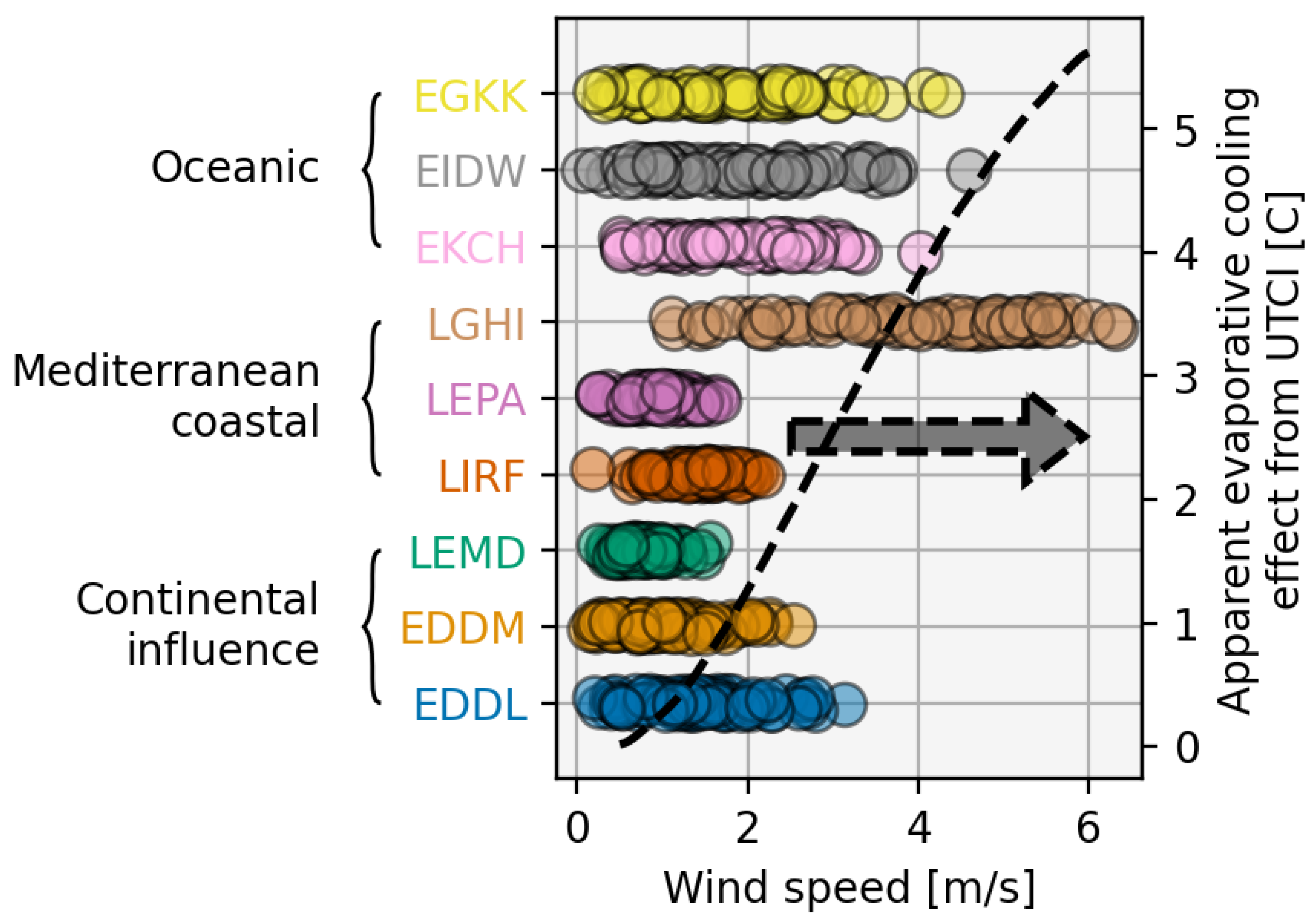
Although we do not explicitly consider the evaporative cooling effect as is included in UTCI, this is not because it is considered negligible, rather due to the absence of reliable, bias-corrected wind data in the present data set. These data are available as raw output from the climate models themselves, however they were not subject to the detailed analysis detailed in Trentini et al. [59]. Future extensions to this work explicitly considering wind are encouraged.
References
- Termeer, C.J.A.M.; Dewulf, A.; Biesbroek, R. A critical assessment of the wicked problem concept: relevance and usefulness for policy science and practice. Policy and Society 2019, 38, 167–179. [Google Scholar] [CrossRef]
- Sun, Z.; Yang, H. The Wicked Problem of Climate Change: A New Approach Based on Social Mess and Fragmentation. Sustainability 2016, 8, 1312. [Google Scholar] [CrossRef]
- Irvine, E.A.; Shine, K.P.; Stringer, M.A. What are the implications of climate change for trans-Atlantic aircraft routing and flight time? Transportation Research Part D: Transport and Environment 2016, 47, 44–53. [Google Scholar] [CrossRef]
- Padhra, A. Emissions from auxiliary power units and ground power units during intraday aircraft turnarounds at European airports. Transportation Research Part D: Transport and Environment 2018, 63, 433–444. [Google Scholar] [CrossRef]
- Ashley, X.M. How Airport Construction will Evolve with the Increased Effects of Climate Change. Beyond: Undergraduate Research Journal 2019, 3, Article 5. [Google Scholar]
- Alahmad, B.; Isachsen, I.; Alwadi, Y.; Taha, H.; Bernheim, A.; Cooke, E.; Wesley, E.; Kats, G.; Spengler, J.D. A modeling study of cool surfaces and outdoor workers productivity at San Francisco International Airport. PNAS Nexus 2025, 4, pgae593. [Google Scholar] [CrossRef]
- Burbidge, R.; Paling, C.; Dunk, R.M. A systematic review of adaption to climate change impacts in the aviation sector. Transport Reviews 2024, 44, 8–33. [Google Scholar] [CrossRef]
- Deshayes, T.A.; Hsouna, H.; Braham, M.A.A.; et al. Work–rest regimens for work in hot environments: A scoping review. American Journal of Industrial Medicine 2024, 67, e23569. [Google Scholar] [CrossRef] [PubMed]
- Torbat Esfahani, M.; Awolusi, I.; Hatipkarasulu, Y. Heat Stress Prevention in Construction: A Systematic Review and Meta-Analysis of Risk Factors and Control Strategies. International Journal of Environmental Research and Public Health 2024, 21, 1681. [Google Scholar] [CrossRef]
- Spector, J.T.; Masuda, Y.J.; Wolff, N.H.; Calkins, M.; Seixas, N.S. Heat Exposure and Occupational Injuries: Review of the Literature and Implications. Current Environmental Health Reports 2019, 6, 286–296. [Google Scholar] [CrossRef]
- Zhao, M.; Lee, J.K.W.; Kjellstrom, T.; Cai, W. Assessment of the economic impact of heat-related labor productivity loss: a systematic review. Climatic Change 2021, 167, 31. [Google Scholar] [CrossRef]
- Sun, Y.; Zhu, S.; Wang, D.; et al. Global supply chains amplify economic costs of future extreme heat risk. Nature 2024, 631, 123–130. [Google Scholar] [CrossRef]
- Hasegawa, T.; Fujimori, S.; Havlík, P.; Valin, H.; Leclère, B.; Riahi, K.; Havlík, P. Quantifying the Economic Impact of Changes in Energy Demand for Space Heating and Cooling. Palgrave Communications 2016, 2, 16013. [Google Scholar] [CrossRef]
- Lizana, J.; et al. Overcoming the Incumbency and Barriers to Sustainable Cooling. Buildings & Cities 2023, 4, 1–20. [Google Scholar] [CrossRef]
- Liu, Q.; Fu, C.; Xu, Z.; Ding, A.; et al. Global warming intensifies extreme day-to-day temperature changes in mid–low latitudes. Nature Climate Change 2025. [Google Scholar] [CrossRef]
- Palu, R.; Mahmoud, H. Impact of climate change on the integrity of the superstructure of deteriorated U.S. bridges. PLOS ONE 2019, 14, e0223307. [Google Scholar] [CrossRef]
- Grose, T.K. Hot & Bothered. ASEE Prism 2022. Published by the American Society for Engineering Education.
- Barbi, S.R.; Labi, S.; Roesler, J.R. Incorporating Climate Change Effects in Airport Pavement Design and Management. Transportation Research Record 2023, 2677, 1–14. [Google Scholar] [CrossRef]
- Williams, J.; Williams, P.D.; Guerrini, F.; Venturini, M. Quantifying the Effects of Climate Change on Aircraft Take-Off Performance at European Airports. Aerospace 2025, 12. [Google Scholar] [CrossRef]
- Williams, J.; Williams, P.D.; Venturini, M.; Padhra, A.; Gratton, G.; Rapsomanikis, S. The Impacts of Climate Change on Aircraft Noise near European Airports. Aerospace 2025, 12. [Google Scholar] [CrossRef]
- Eyring, V.; Bony, S.; Meehl, G.A.; Senior, C.A.; Stevens, B.; Stouffer, R.J.; Taylor, K.E. Overview of the Coupled Model Intercomparison Project Phase 6 (CMIP6) Experimental Design and Organization. Geoscientific Model Development 2016, 9, 1937–1958. [Google Scholar] [CrossRef]
- Cinquini, L.; Crichton, D.; Mattmann, C.; Harney, J.; Shipman, G.; Wang, F.; Ananthakrishnan, R.; Miller, N.; Denvil, S.; Morgan, M.; et al. The Earth System Grid Federation: An open infrastructure for access to distributed geospatial data. Future Generation Computer Systems 2014, 36, 400–417. [Google Scholar] [CrossRef]
- van Vuuren, D.P.; Riahi, K.; Calvin, K.V.; Dellink, R.; Emmerling, J.; Fujimori, S.; KC, S.; Kriegler, E.; O’Neill, B.C. The Shared Socio-economic Pathways: Trajectories for human development and global environmental change. Global Environmental Change 2017, 42, 267–281. [Google Scholar] [CrossRef]
- Ahmed, M.; Seraj, R.; Islam, S.M.S. The k-means Algorithm: A Comprehensive Survey and Performance Evaluation. Electronics 2020, 9, 1295. [Google Scholar] [CrossRef]
- Peel, M.C.; Finlayson, B.L.; McMahon, T.A. Updated world map of the Köppen-Geiger climate classification. Hydrology and Earth System Sciences 2007, 11, 1633–1644. [Google Scholar] [CrossRef]
- Błażejczyk, K.; Jendritzky, G.; Bröde, P.; Fiala, D.; Havenith, G.; Epstein, Y.; Psikuta, A.; Kampmann, B. An introduction to the Universal Thermal Climate Index (UTCI). Geographia Polonica 2013, 86, 5–10. [Google Scholar] [CrossRef]
- Brimicombe, C.; Lo, C.H.B.; Pappenberger, F.; Di Napoli, C.; Maciel, P.; Quintino, T.; Cornforth, R.; Cloke, H.L. Wet Bulb Globe Temperature: Indicating Extreme Heat Risk on a Global Grid. GeoHealth 2023, 7, e2022GH000701. [Google Scholar] [CrossRef] [PubMed]
- Masterton, J.M.; Richardson, F.A. Humidex: A Method of Quantifying Human Discomfort Due to Excessive Heat and Humidity. Technical Report En57-23/1, Atmospheric Environment Service, Environment Canada, Downsview, Ontario, 1979.
- Wallace, J.M.; Hobbs, P.V. Atmospheric Science: An Introductory Survey, 2 ed.; Elsevier Academic Press: Amsterdam, 2006.
- Explosive atmospheres – Part 10-1: Classification of areas – Explosive gas atmospheres, 2020. International Electrotechnical Commission, IEC 60079-10-1, 3.0 edition, Geneva, Switzerland.
- Petri, Y.; Caldeira, K. Impacts of global warming on residential heating and cooling degree-days in the United States. Scientific Reports 2015, 5, 12427. [Google Scholar] [CrossRef]
- Harvey, L.D. Using modified multiple heating-degree-day (HDD) and cooling-degree-day (CDD) indices to estimate building heating and cooling loads. Energy and Buildings 2020, 229, 110475. [Google Scholar] [CrossRef]
- Ramon, D.; Allacker, K.; De Troyer, F.; Wouters, H.; van Lipzig, N.P. Future heating and cooling degree days for Belgium under a high-end climate change scenario. Energy and Buildings 2020, 216, 109935. [Google Scholar] [CrossRef]
- Miranda, N.D.; Lizana, J.; Sparrow, S.N.; Zachau-Walker, M.; Watson, P.A.G.; Wallom, D.C.H.; Khosla, R.; McCulloch, M. Change in cooling degree days with global mean temperature rise increasing from 1.5°C to 2.0°C. Nature Sustainability 2023, 6. [Google Scholar] [CrossRef]
- Deroubaix, A.; et al. Large Uncertainties in Trends of Energy Demand for Heating and Cooling Under Climate Change. Nature Communications 2021, 12, 25504. [Google Scholar] [CrossRef]
- Perkins, S.E.; Alexander, L.V. On the Measurement of Heat Waves. Journal of Climate 2013, 26, 4500–4517. [Google Scholar] [CrossRef]
- Bunting, W.; et al. What is a heat wave: A survey and literature synthesis of heat wave definitions across the United States. PLOS Climate 2024, 3, e0000468. [Google Scholar] [CrossRef]
- Zhao, J.J.; Leyva, E.W.; Wong, K.A.; Kataoka-Yahiro, M.; Saligan, L.N. Heat Stress and Determinants of Kidney Health Among Agricultural Workers in the United States: An Integrative Review. International Journal of Environmental Research and Public Health 2025, 22, 1268. [Google Scholar] [CrossRef]
- Rifkin, D.I.; Long, M.W.; Perry, M.J. Climate change and sleep: A systematic review of the literature and conceptual framework. Sleep Medicine Reviews 2018, 42, 3–9. [Google Scholar] [CrossRef] [PubMed]
- Habibi, P.; Razmjouei, J.; Moradi, A.; Mahdavi, F.; Fallah-Aliabadi, S.; Heydari, A. Climate change and heat stress resilient outdoor workers: findings from systematic literature review. BMC Public Health 2024, 24, 19212. [Google Scholar] [CrossRef]
- Molina, M.O.; Soares, P.M.M.; Lima, M.M.; et al. Updated insights on climate change-driven temperature variability across historical and future periods. Climatic Change 2025, 178, 97. [Google Scholar] [CrossRef]
- Saifudeen, A.; Mani, M. Adaptation of Buildings to Climate Change: An Overview. Frontiers in Built Environment 2024, 10, 1327747. [Google Scholar] [CrossRef]
- Yang, R.; Zhan, C.; Sun, L.; Shi, C.; Fan, Y.; Wu, Y.; Yang, J.; Liu, H. Modelling the reflective cracking features of asphalt overlay for airport runway under temperature and airplane load coupling factors. Construction and Building Materials 2024, 403, 138774. [Google Scholar] [CrossRef]
- Hourdin, F.; Mauritsen, T.; Gettelman, A.; Golaz, J.C.; Balaji, V.; Duan, Q.; Folini, D.; Ji, D.; Klocke, D.; Qian, Y.; et al. The Art and Science of Climate Model Tuning. Bulletin of the American Meteorological Society 2017, 98, 589–602. [Google Scholar] [CrossRef]
- Burt, S. Evaluation and verification of new UK air temperature extremes during the July 2022 heatwave. Part 1: maximum temperatures. Weather 2025, 80, 70–78. [Google Scholar] [CrossRef]
- Nazarenko, L.S.; Tausnev, N.; Russell, G.L.; et al. Future Climate Change Under SSP Emission Scenarios With GISS-E2.1. Journal of Advances in Modeling Earth Systems 2022, 14, e2021MS002871. [Google Scholar] [CrossRef]
- Tollefson, J. Earth breaches 1.5°C climate limit for the first time: what does it mean? Nature 2025, 625, 10–11. [Google Scholar] [CrossRef] [PubMed]
- Mehmood, A.; et al. Integrating Latent Load into the Cooling Degree Days Concept. Buildings 2024, 14, 106. [Google Scholar] [CrossRef]
- Cao, J.; Li, M.; et al. An efficient climate index for reflecting cooling energy consumption: Cooling degree days based on wet bulb temperature. Meteorological Applications 2021, 28, e2005. [Google Scholar] [CrossRef]
- Bhatnagar, M. Determining base temperature for heating and cooling degree-days for India. Journal of Building Engineering 2018, 18, 293–304. [Google Scholar] [CrossRef]
- Parker, D.E.; Legg, T.P.; Folland, C.K. A new daily Central England Temperature Series, 1772–1991. International Journal of Climatology 1992, 12, 317–342. [Google Scholar] [CrossRef]
- Liu, J.; Qi, J.; Yin, P.; Liu, W.; He, C.; Gao, Y.; Zhou, L.; Zhu, Y.; Kan, H.; Chen, R.; et al. Rising cause-specific mortality risk and burden of compound heatwaves amid climate change. Nature Climate Change 2024, 14. Published online: 17 September 2024. [CrossRef]
- IEA. Climate resilience – Power Systems in Transition. https://www.iea.org/reports/power-systems-in-transition/climate-resilience, 2020. Licence: CC BY 4.0.
- Croce, P.; Formichi, P.; Landi, F. Climate Change: Impacts on Climatic Actions and Structural Reliability. Applied Sciences 2019, 9, 5416. [Google Scholar] [CrossRef]
- Voskaki, A.; Budd, L.; Mason, K. The impact of climate hazards to airport systems: a synthesis of the implications and risk mitigation trends. Transport Reviews 2023, 43, 216–239. [Google Scholar] [CrossRef]
- Williams, P.D. Increased light, moderate, and severe clear-air turbulence in response to climate change. Advances in atmospheric sciences 2017, 34, 576–586. [Google Scholar] [CrossRef]
- Singh, D.K.; Sanyal, S.; Wuebbles, D.J. Understanding the role of contrails and contrail cirrus in climate change: a global perspective. Atmospheric Chemistry and Physics 2024, 24, 9219–9262. [Google Scholar] [CrossRef]
- Tartarini, F.; Schiavon, S. pythermalcomfort: A Python package for thermal comfort research. SoftwareX 2020, 12, 100578. [Google Scholar] [CrossRef]
- Trentini, L.; Venturini, M.; Guerrini, F.; Gesso, S.D.; Calmanti, S.; Petitta, M. Identifying Climate Extremes in Southern Africa through Advanced Bias Correction of Climate Projections. Bulletin of Atmospheric Science and Technology 2025, 6. [Google Scholar] [CrossRef]
Figure 1.
The subset of 9 airports chosen to better visually represent the larger 30 airport ensemble. The blue region represents oceanically-controlled sites, the green regions shows those with a large continental influence and the red region shows those of a coastal Mediterranean nature. Precise coordinates are given in Table 2.
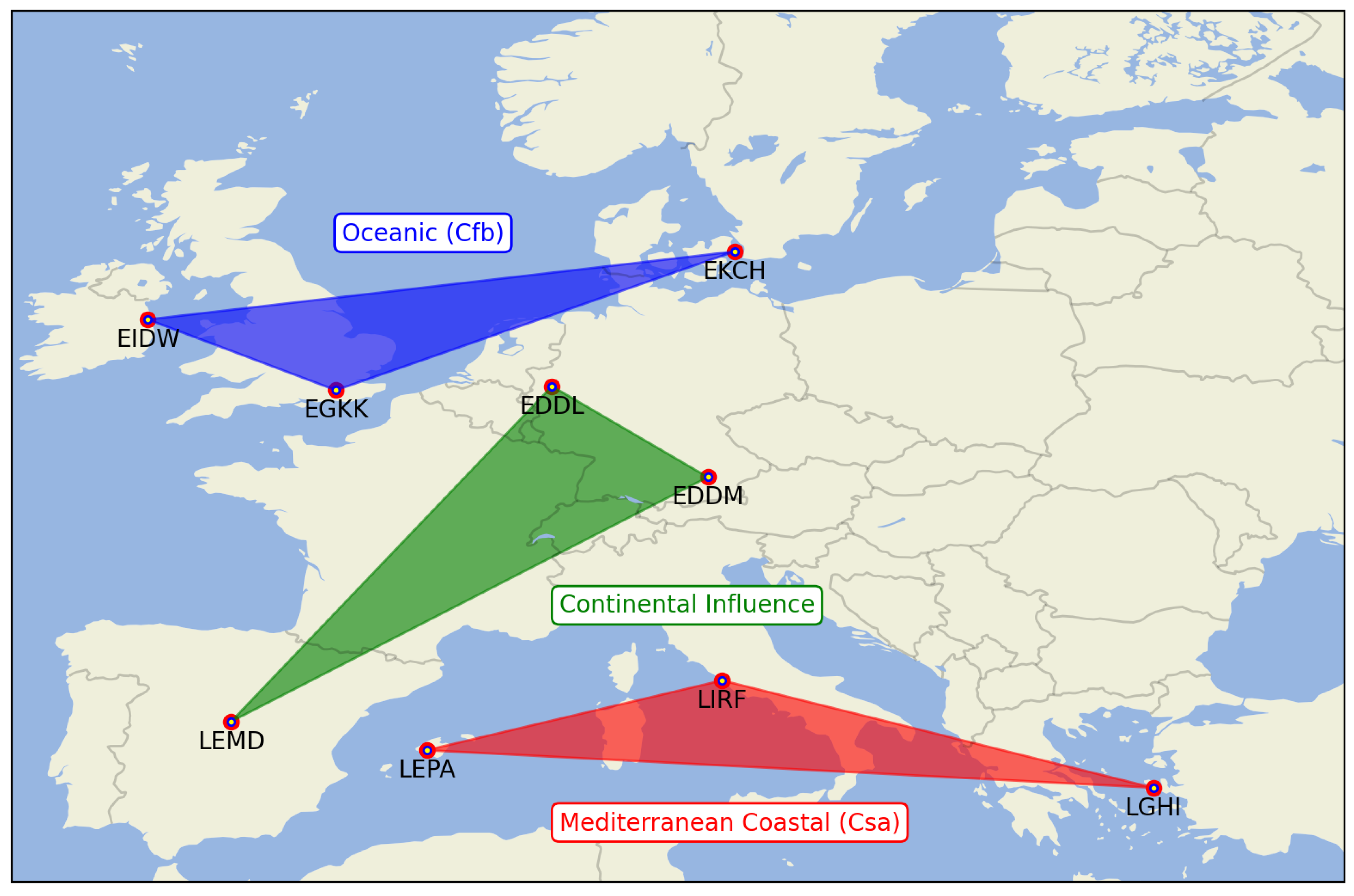
Figure 2.
A representative illustration of Humidex (in ° Celsius) as a function of dry bulb temperature and specific humidity. The vapour pressure is calculated using Equation (1) and a pressure of 1015hPa. In extreme conditions (i.e. high temperature and humidity) the difference between the dry bulb temperature and that due to water vapour can exceed 6°.
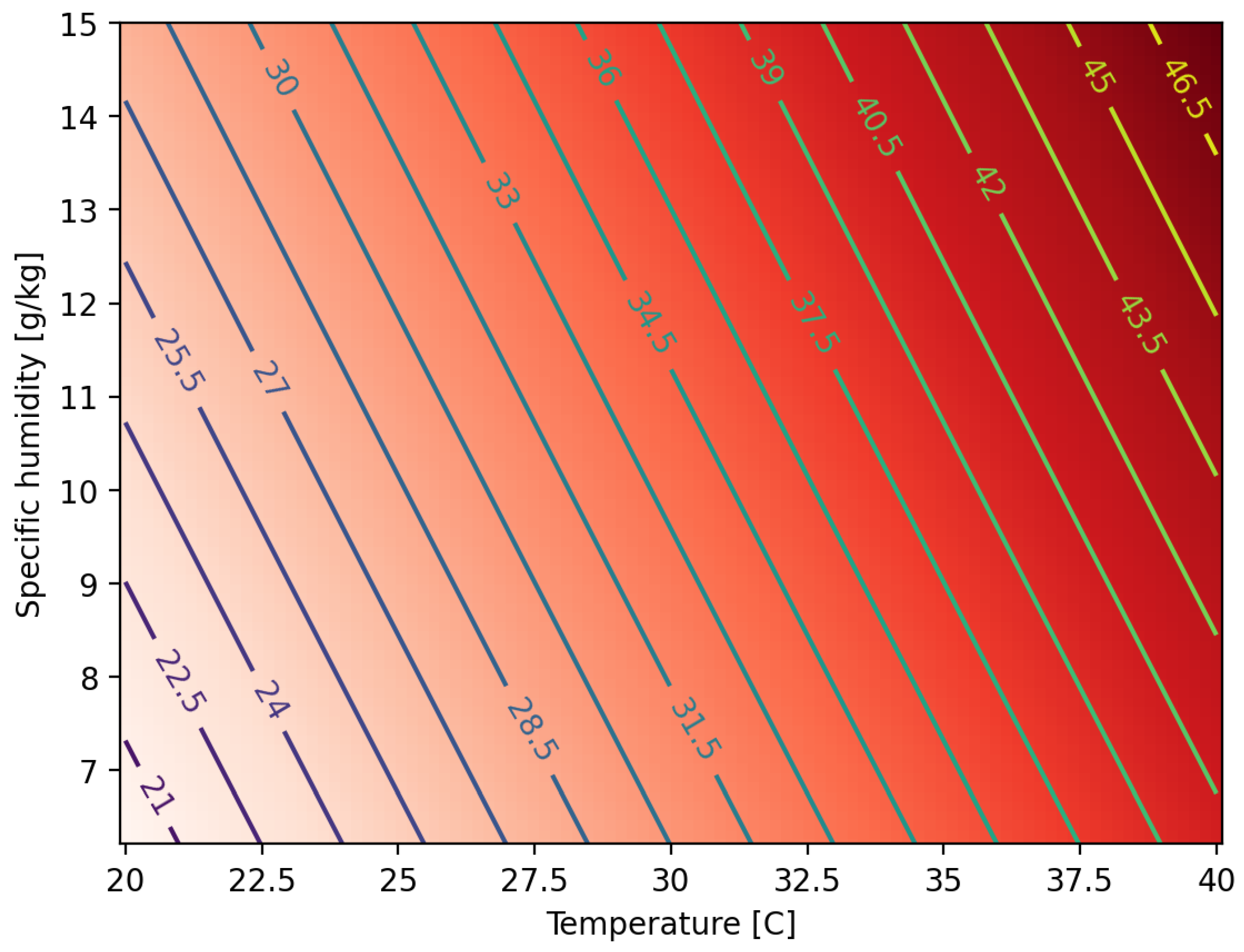
Figure 3.
box-and-whisker plots of Humidex , H, for each of the airports shown in Figure 1 and for each SSP scenario. The coloured horizontal lines and the text on the right hand side illustrate the pre-defined levels of comfort shown in Table 3. The three climate regimes are shown, separated by vertical dashed lines.
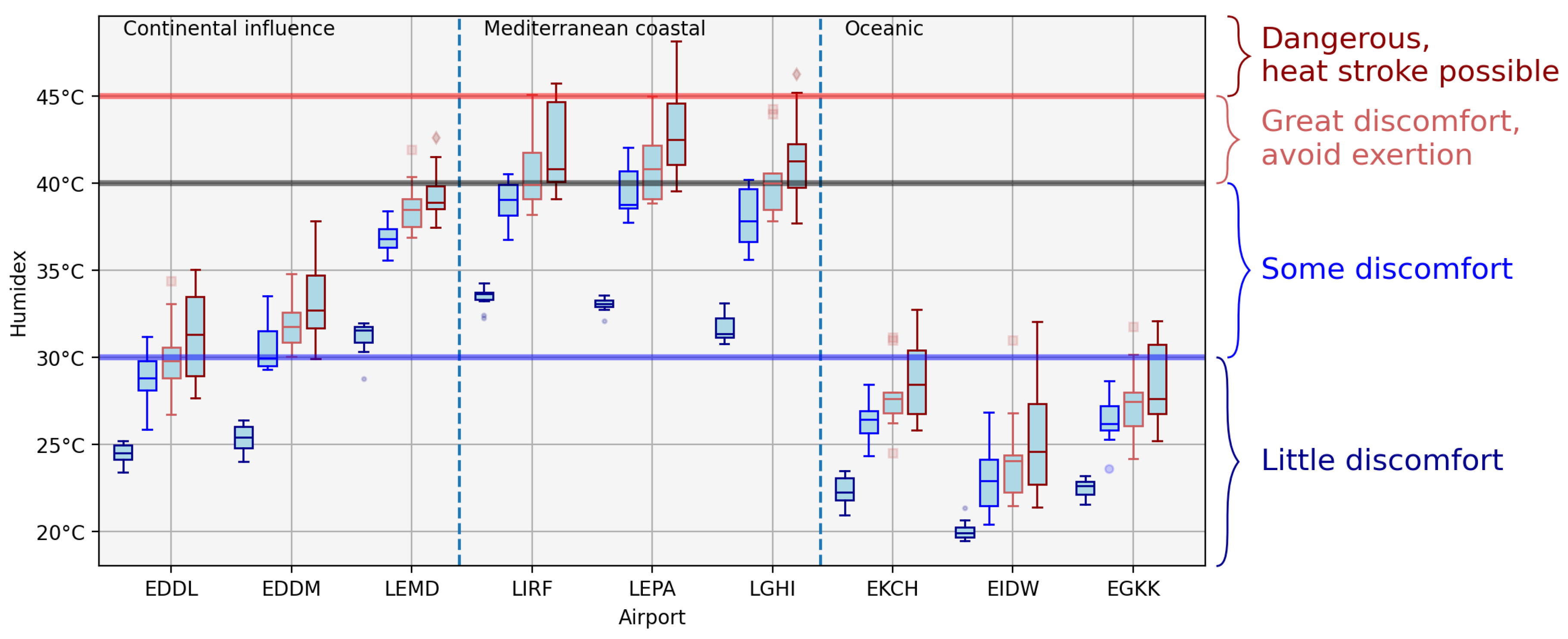
Figure 4.
Probability of maximum daily JJA temperature exceeding the flash point of kerosene. The box and whisker plots show the intra-ensemble variability and the historical, SSP1, 3 and 5 results are shown in dark blue, blue, red, and dark red respectively. The three climate regimes are shown, separated by vertical dashed lines.
Figure 5.
Number of Cooling degree days for each SSP. The box and whisker plots show the intra-ensemble variability and the SSP1, 3 and 5 results are shown in blue, red, and dark red respectively. The three climate regimes are shown, separated by vertical dashed lines.
Figure 5.
Number of Cooling degree days for each SSP. The box and whisker plots show the intra-ensemble variability and the SSP1, 3 and 5 results are shown in blue, red, and dark red respectively. The three climate regimes are shown, separated by vertical dashed lines.
Figure 6.
Heating degree days for each SSP. The box and whisker plots show the intra-ensemble variability and the SSP1, 3 and 5 results are shown in blue, red, and dark red respectively. The three climate regimes are shown, separated by vertical dashed lines.
Figure 6.
Heating degree days for each SSP. The box and whisker plots show the intra-ensemble variability and the SSP1, 3 and 5 results are shown in blue, red, and dark red respectively. The three climate regimes are shown, separated by vertical dashed lines.
Figure 7.
The number of heatwaves experienced by each site where a heatwave is defined as a 3-or-more day period of daily mean 2m temperatures exceeding the 95th percentile of the historical simulations for each model respectively. The box and whisker plots show the intra-model ensemble variability and the historical, SSP1, 3 and 5 results are shown in dark blue, blue, red, and dark red respectively. The three climate regimes are shown, separated by vertical dashed lines and the yellow horizontal is the 1985-2014 JJA heatwave occurrence from the Central England Data set.
Figure 8.
(a-i) (percentile-percentile) plots are shown by the blue ‘plus’ symbols where the extents of the arms in each axial direction show the respective inter-model spread. The historical data is on the x axis and the y axis shows the SSP5-8.5 results. The diagonal line () shows the line that would be made by the plots if the distributions were identical. The solid line is the deviation from the line on the same y-axis scale. (a-c) are continentally influenced; (d-f) are Mediterranean coastal; (g-i) are oceanic. Note that the green lines in (c) and (i) show large and small amounts of deviation from respectively; (j) and (k) show the Gaussian kernel density estimate distributions (and standard errors, ). The x-axis ranges of the KDE plots is chosen to match the historical Q ranges in (c) and (i) respectively.
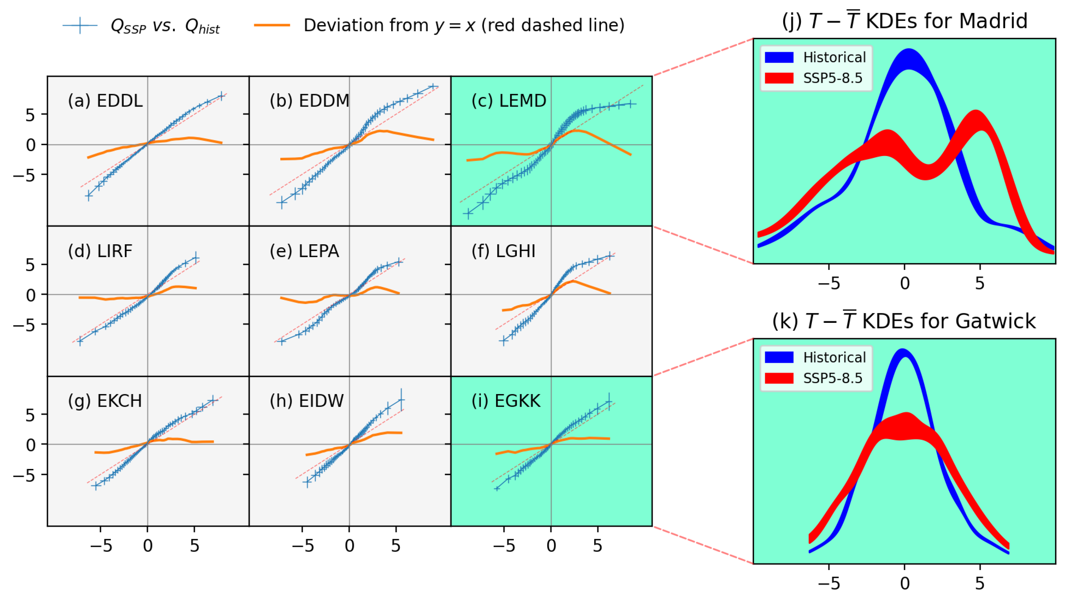

Table 1.
Shared Socioeconomic Pathways – SSPs – used, see van Vuuren et al. [23] for more details.
Table 1.
Shared Socioeconomic Pathways – SSPs – used, see van Vuuren et al. [23] for more details.
| Scenario name | Detail | Description |
|---|---|---|
| SSP1-2.6 | • ‘Sustainable development’ • 2.6 W· top-of-atmosphere forcing at 2100 |
Low level of climate change |
| SSP3-7.0 | • ‘Regional rivalry’ • 7.0 W· top-of-atmosphere forcing at 2100 |
Medium level of climate change |
| SSP5-8.5 | • ‘Fossil-fuelled’ development • 8.5 W· top-of-atmosphere forcing at 2100 |
High level of climate change |
Table 2.
The subset of 9 airports used in the results figures below and shown in Figure 1.
Table 2.
The subset of 9 airports used in the results figures below and shown in Figure 1.
| Airport | ICAO code | Climate classification (Köppen) | Latitude, Longitude |
|---|---|---|---|
| Dublin | EIDW | Oceanic (Cfb) | 53.4213°, -6.27007° |
| London Gatwick | EGKK | Oceanic (Cfb) | 51.1481° , -0.19028° |
| Copenhagen Kastrup | EKCH | Oceanic (Cfb) | 55.6179° , 12.656° |
| Düsseldorf | EDDL | Continental influence | 51.2895° , 6.76678° |
| Munich | EDDM | Continental influence | 48.3538° , 11.7861° |
| Madrid Barajas | LEMD | Continental influence | 40.4936° , -3.56676° |
| Palma De Mallorca | LEPA | Mediterranean coastal (Csa) | 39.5517° , 2.73881° |
| Rome (Fiumicino) | LIRF | Mediterranean coastal (Csa) | 41.8045° , 12.2508° |
| Chios Island National | LGHI | Mediterranean coastal (Csa) | 38.3432° , 26.1406° |
Table 3.
Qualitative Humidex level descriptions . Note that in the calculations below, we ensure that the levels are contiguous with the boundaries at 30, 40 and 45°C.
Table 3.
Qualitative Humidex level descriptions . Note that in the calculations below, we ensure that the levels are contiguous with the boundaries at 30, 40 and 45°C.
| Humidex Range [°C] | Degree of Comfort |
|---|---|
| 20-29 | Little discomfort |
| 30-39 | Some discomfort |
| 40-45 | Great discomfort; avoid exertion |
| 46 and over | Dangerous; heat stroke possible |
Disclaimer/Publisher’s Note: The statements, opinions and data contained in all publications are solely those of the individual author(s) and contributor(s) and not of MDPI and/or the editor(s). MDPI and/or the editor(s) disclaim responsibility for any injury to people or property resulting from any ideas, methods, instructions or products referred to in the content. |
© 2025 by the authors. Licensee MDPI, Basel, Switzerland. This article is an open access article distributed under the terms and conditions of the Creative Commons Attribution (CC BY) license (http://creativecommons.org/licenses/by/4.0/).
Copyright: This open access article is published under a Creative Commons CC BY 4.0 license, which permit the free download, distribution, and reuse, provided that the author and preprint are cited in any reuse.


