Submitted:
22 December 2025
Posted:
23 December 2025
Read the latest preprint version here
Abstract
Performance based evaluation of reinforced soil retaining structures often relies on numerical analyses that demand substantial time and expert effort, largely due to the complex interactions among soils, reinforcements, facings, and seismic loading. This study introduces an efficient approach for developing seismic resisting capacity curves for geosynthetic reinforced slopes with rigid facings, using a computer program built on the Force Equilibrium based Finite Displacement Method (FFDM). Positioned between conventional, non performance based limit equilibrium methods (LEM) and the more computationally intensive finite element method (FEM), the FFDM offers a practical platform for performance based seismic assessment in engineering design. The method is demonstrated through a re examination of the Tanada Wall, a geosynthetic reinforced soil retaining wall with a full-height rigid panel facing (GRS-FHR) that experienced strong shaking during the 1995 Hyogoken Nambu earthquake (ML = 7.2). Using only parameters available in published databases, the FFDM generates realistic seis-mic resistance curves and directly computes seismic displacements. Three advantages distinguish the FFDM from traditional LEM based Newmark approaches: (1) explicit incorporation of peak soil strength and post peak degradation along the slip surface, eliminating the need for empirical “operational” strength adjustments; (2) direct use of peak ground acceleration (HPGA/g) as input, avoiding reliance on empirically selected seismic coefficients; and (3) capability for back analysis, enabling soil strength and de-formation parameters to be calibrated from small observed displacements (on the order of 10⁻³ m) during medium scale earthquakes and subsequently used to predict structural response under more severe ground shaking.
Keywords:
finite displacement method (FFDM)
; performance-based seismic evaluation
; geosynthetic-reinforced soil structures
; nonlinear soil model
; seismic resistance curves
1. Introduction
In conventional engineering practice, the seismic stability of slopes is commonly evaluated using the safety factor (Fs) derived from prescribed seismic coefficients (kh) through limit equilibrium methods (LEM). To estimate seismic-induced slope displacements, Newmark’s hybrid approach—described in [1]—combines LEM with sliding-block dynamics and remains widely adopted. A key requirement for applying Newmark’s method is the determination of a calibrated critical seismic coefficient (khc), obtained from the Fs–kh relationship at the condition Fs = 1.0. Identifying this khc typically involves iterative trial-and-error adjustments to determine an “operational” internal friction angle (φ) that produces a satisfactory Fs–kh curve.
To reduce the empiricism and iterative calibration inherent in this conventional workflow, Huang’s Force-equilibrium-based Finite Displacement Method (FFDM), described in [2,3], was developed. By integrating soil stress–displacement behavior and displacement compatibility within the sliding mass into the fundamental force and moment equilibrium framework of LEM, the FFDM provides a more direct and rational means of evaluating displacement-based slope performance. The method has since been successfully applied to groundwater induced landslides and reinforced slopes subjected to pseudo static seismic loading. Its capability has further been demonstrated through back-calculation of displacement-based soil and weathered-rock parameters [4,5] as well as through predictions of slope displacements [6].
Building on these developments, the present study aims to derive displacement-based seismic resisting capacity curves for a full scale geosynthetic reinforced railway embankment with a rigid concrete facing (referred to as the Tanada wall). The analyses are performed using SLOPE ffdm 2.0 [7], a computer program that integrates both conventional LEM-based and displacement-based FFDM analytical tools.
2. Methodology and Materials
2.1. Hyperbolic Soil Stress-Displacement Model
As illustrated in Figure 1, a hyperbolic model describing the normalized shear stress (τ/τf)–shear displacement (Δ) response along the potential failure surface was proposed in [2]. This model is an adaptation of the well known hyperbolic relationship for shear stress–strain behavior developed in [8].
τ/τf = ∆ / (a+b∙∆)
Where, a = τf / kinitial, b = Rf, Rf = τf / τult
- kinitial: Initial shear stiffness of soils
- τult: Asymptote strength at infinite displacement
- τf: Shear strength of soil according to the Mohr-Coulomb failure criterion
- Rf: Asymptote strength ratio (= τf / τult)
The shear strength of soils (τf) is defined by the Mohr-Coulomb failure criterion:
τf = c + σ'n ∙ tan ϕ
- σn’: Effective normal stress
- : Cohesion intercept
- φ: Internal friction angle of soils
2.2. Multi-Wedge Failure Mechanism
Figure 2 illustrates the multi wedge failure mechanism adopted in this study. This mechanism evolved from the classical “two-wedge” or “bi-linear” failure model, which has long been used to simulate the failure of engineered slopes with steep faces, such as mechanically stabilized earth (MSE) walls and geosynthetic reinforced slopes with rigid or near vertical facings. An enhanced version of the two wedge mechanism was proposed in [9], comprising two active wedges (Wedges 1 and 2), a facing column, and—when present—a passive wedge located beneath the toe of the facing. This multi wedge formulation provides deeper insight into the contribution of the facing system to overall slope stability. Its advantages are further amplified when combined with the FFDM, which enables displacement based performance evaluation of the slope. Figure 3 presents the body forces and reaction forces acting on a generalized polygon wedge configuration. Triangular wedges, exemplified by Wedges 1 and 4, constitute special cases where the soil strength and reaction forces along one boundary are assumed to be negligible or zero.
By applying force equilibrium in both horizontal (x) and vertical (y) directions, the reaction force on the left side of each wedge can be expressed as:
Re = f (Rb, Rr, Tr, Tb, Te, Ce,Cr, Cb, Ce, ϕr, ϕb, ϕe, kh, kv, Qv, Qh)
Where, Cr = c ∙ lr / FSi , Cb = c ∙ lb / FSi , Ce = c ∙ le / FSi
ϕr = tan-1(tan ϕ / FSi), ϕb = tan-1(tan ϕ / FSi) , ϕe = tan-1(tan ϕ / FSi)
- Cr, Cb, Ce: cohesive resistance along soil-block interfaces
- lr, lb, le: lengths of soil-block interfaces
- ϕr, ϕb, ϕe:mobilized internal friction angles at interfaces
- Tr, Tb, Te: reinforcement force at at interfaces
- Rr, Rb: reaction forces at interfaces
To determine the reaction force acting on the left side of each wedge in the LEM analysis, the computation advances sequentially from wedge 1 to wedge 3 (or wedge 4, if present). A constant safety factor, Fs, is assumed and applied uniformly to all wedges. With this assumption, all terms on the right-hand side of the governing force-equilibrium relationship are known except for the base reaction force Rb. Because both horizontal and vertical force equilibrium are imposed, the system is statically determinate. The safety factor is updated through iterative equilibrium calculations, typically starting with an initial trial value of Fs = 1.0, and is adjusted until the virtual external force Re on the left side of wedge 3 (or wedge 4) becomes negligibly small, e.g., Re < 0.1 kN.
In contrast, when the same governing relationship is solved within the FFDM framework, the safety factor for each soil block (FSi) and the mobilized reinforceemnt force (Tr, Tb, Te) depends on its displacement (Δi). The system remains statically determinate, but the safety factor is updated continuously according to the displacement field at the block base and along the interfaces. The computation begins by imposing a small vertical displacement at the crest of wedge 1 (Δ0), e.g. a vertical displacement of 0.001m, and proceeds until all force equilibrium requirements are satisfied.
2.3. Post-Peak Stress-Displacement Relationship
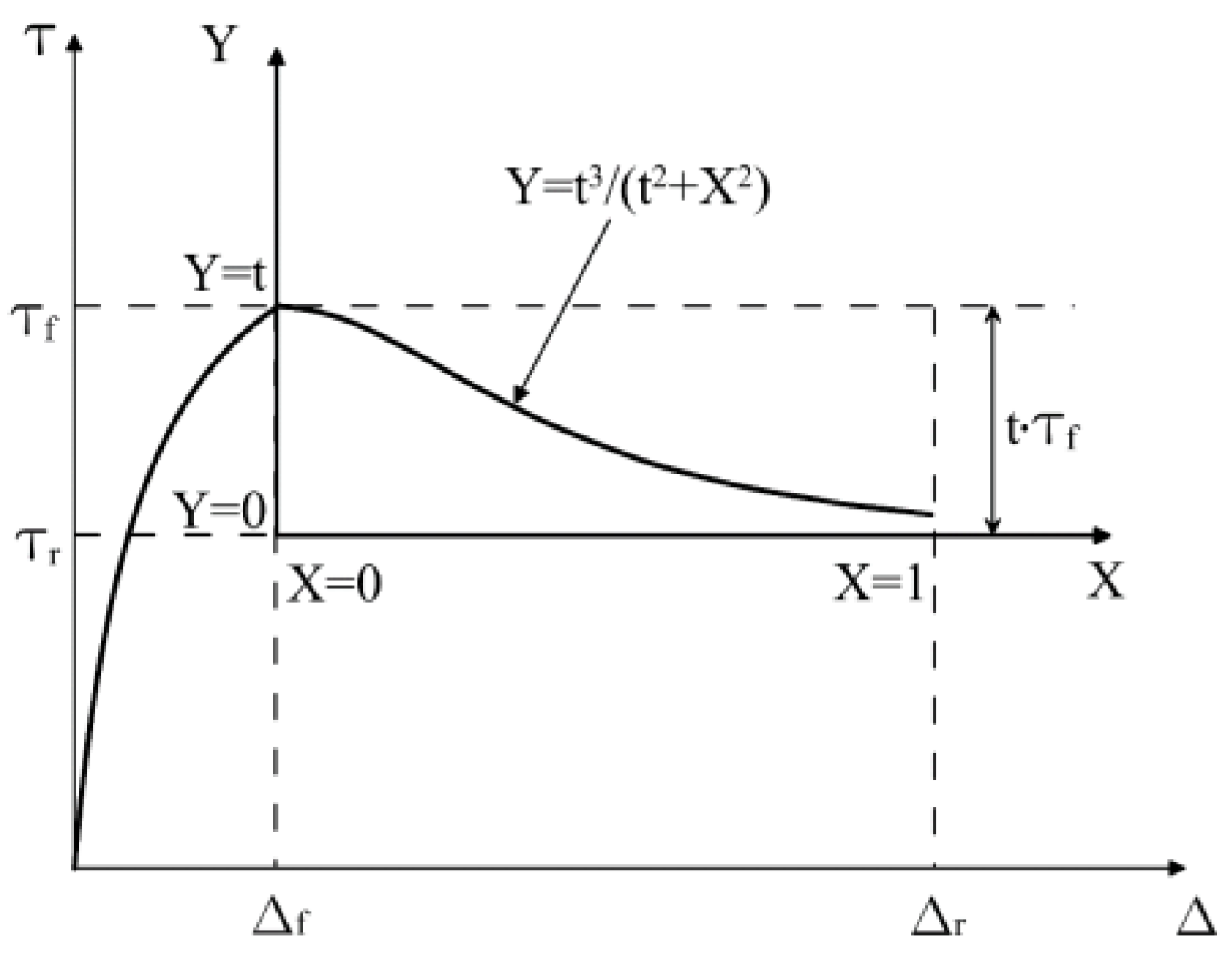
The post-peak segment of the shear stress–displacement (τ–Δ) curve is modeled using the Versoria (or Witch of Agnesi) curve [6,10], schematically illustrated in Fig. 4. For efficient integration into the overall stress–displacement framework, a normalized local coordinate system (X–Y) is adopted. The X-axis origin (X = 0) aligns with the peak stress point (τf). The Y-axis origin (Y = 0) corresponds to the asymptotic value of the residual stress (τr). A distinctive feature of this curve is that the residual state (τr) is theoretically reached at an infinite Δ. In practice, however, a finite displacement (Δr), observed experimentally at the onset of the residual state (defined at X = 1), can be used to approximate τr with a negligibly small error (normally less than 1% error). The shear strength in the post-peak regime (τpost-peak) can be expressed as:
τpost-peak = τf - τf ∙ (t - Y ) = τf ∙ (1- t + Y )
Y = t3 / ( t2 +X2 )
X= (Δ - Δf ) / (Δr - Δf )
t = (τf -τr ) ∙ τf
Δr = Δf ∙ Δratio
- t: normalized strength reduction between peak and residual states
- Y: normalized post-peak shear stress
- X: normalized post-peak shear displacement
- Δf: shear displacement at peak stress state
- Δr: shear displacement at the entrance of residual state
- Δratio: residual-to-peak displacement ratio
Figure 4.
A transformed coordinate system of the ‘Versoria’ curve for post-peak stress-displacement relationships.
Figure 4.
A transformed coordinate system of the ‘Versoria’ curve for post-peak stress-displacement relationships.
When the post-peak state is considered in the slope-displacement analysis using SLOPE-ffdm 2.0, Eq. (4) is applied to update the available soil strength along the slip surface whenever the condition Δ > Δf is detected during the iterative displacement computations.
2.4. Displacement Compatibility
A hodograph (displacement diagram) that satisfies displacement compatibility - as schematically illustrated in Figure 5 - is derived following the approach in [11]. This formulation maintains displacement compatibility across soil interfaces and forms the basis for kinematic analysis of the sliding block system. The displacement at soil wedge (or slice) i can be expressed as:
Δi = Δ0 ∙ f (αi)
f (αi) = cos (α1 -2Ψ) /[sin (α1 -Ψ) ∙ cos ( 2Ψ- α1)]
2.5. Displacement Increment
To evaluate slope displacements resulting from changes in external or internal conditions—such as seismic loading, variations in the water table, or pore water pressure—two displacement values for each slice (Δᵢ) are calculated: one representing the state prior to the event and the other representing the state afterward. The displacement increments for slice i, induced by the change in stress conditions, is schematically illustrated in Figure 6 and defined as:
Δi = Δbi - Δai
2.6. The Tanada Wall
The Tanada wall is a geosynthetic-reinforced soil retaining wall with a full-height rigid panel facing (GRS-FHR), also known as a RRR wall. It formed part of a railway embankment located in a severely shaken area during the 1995 Hyogoken-Nambu earthquake (sometimes referred to as the Kobe earthquake; ML = 7.2). Despite severe damage to nearby houses and soil-retaining structures, the Tanada wall demonstrated remarkable seismic resistance, with recorded displacements of only 0.1 m at the toe and 0.26 m at the top, as illustrated in Figure 8. Comprehensive post-earthquake investigations and analyses were conducted in [12,13]. Based on site observations, the horizontal peak ground acceleration (HPGA) in the vicinity of the Tanada wall was estimated to be approximately 0.8 g in [12] (where g denotes gravitational acceleration).
Figure 7.
Cross-section of the Tanada wall following the earthquake [12].
Figure 7.
Cross-section of the Tanada wall following the earthquake [12].
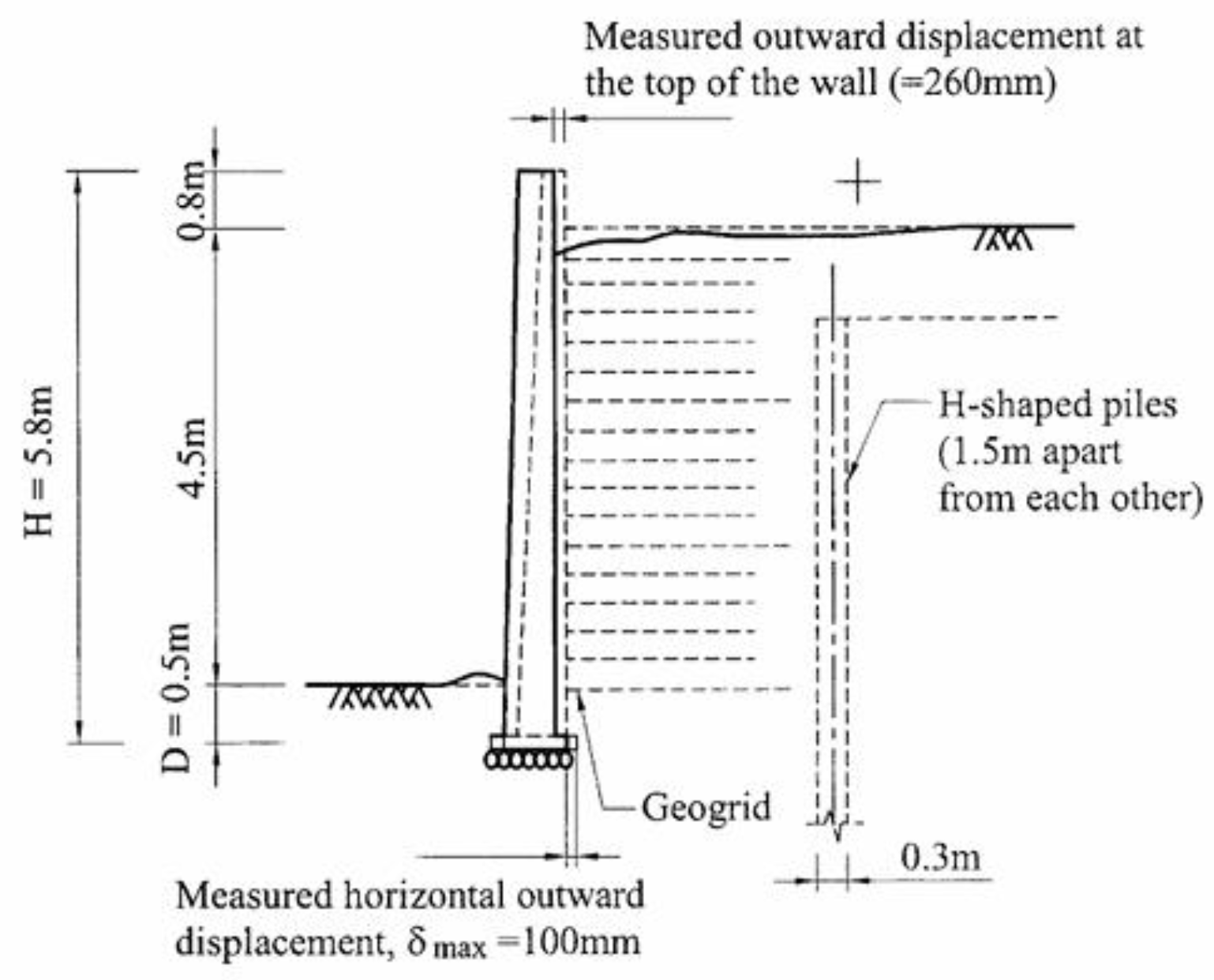
Figure 8.
Integrated pre- and post-peak stress-displacement curves for the displacement analyses.
2.7. Material Properties
The material properties used in the subsequent FFDM analyses of the Tanada wall are summarized in Table 1. Key evaluations for several primary input parameters that significantly influence seismic displacements are outlined below:
(1) Peak strengths of soils, cpeak, ϕpeak: High-quality, cohesionless backfill (cpeak= 0) was clearly used in constructing the Tanada wall, a crucial component of the railway embankment. When applying the hyperbolic soil model, the design value of internal friction angle, ϕ= 40°is adopted [12]. This value is considered as an ‘operational’ internal friction angle, slightly conservative in nature. In contrast, when incorporating the post-peak model for slope displacement evaluation, a higher ϕpeak= 45° - approximately 10% greater than the design value - is used to reflect the superior backfill quality and compaction during embankment construction. In the post-peak condition, cohesion is consistently zero, and the residual friction angle is taken as ϕres ≅ 0.9ϕpeak in the case study.
(2) Shear stiffness number, K: The analysis adopts stiffness values of K = 200 and K = 400, derived from a database of large- and medium-sized direct shear tests [6,15]. These values represent the lower-bound and median values for φ = 40° within the dataset.
(3) Displacement-dependent reinforcement pullout model: The mobilized reinforcement force at the soil–block interface is determined using the hyperbolic reinforcement pullout model described in [3]. The peak adhesion at the soil–reinforcement interface is cs–r = 0, and the peak friction angle is φs–r = 40°. It is assumed that this interface friction angle is not less than the internal friction angle of the backfill, as the reinforcement is a geogrid with woven junctions. The hyperbolic model parameters for reinforcement pullout - derived from a pullout test database - include pullout stiffness number Kₜ = 10, stress dependency exponent nₜ= 0.1, and strength ratio Rₜ= 0.7 (failure strength / asymptotic strength).
(4) Tie-Break Strength of Reinforcement: In the FFDM hyperbolic reinforcement pullout model, the tie-break strength Ttie-break= 30 kN/m is defined as the unfactored ultimate tensile strength of the geogrid, reflecting the high-quality construction practices employed during the original project. This definition contrasts with the factored allowable tensile strength commonly used in conventional limit-equilibrium methods.
(5) Post-Peak Soil Stress–Displacement Model: The post-peak cohesion is consistently zero (cᵣₑₛ= 0), while the residual friction angle is taken as φᵣₑₛ ≈ 0.9φₚₑₐₖ= 41° in the case study. A residual displacement ratio of Δᵣ/Δf = 5.0 is used, following the post-peak soil stress–displacement studies reported in [6,15]. Results of the studies reveal that typical dense sand exhibit Δᵣ/Δf between 2.5 and 6.0.
(6) The H-piles located behind the wall at 1.5-meter center-to-center spacing were excluded. Due to their slenderness and wide spacing, they permit effective transmission of seismic earth pressure and thus do not significantly influence the results.
(7) The inter-block strength ratio (finter-block) defined as the ratio between the full shear strength to the shear strength available at the block-block interface in the force equilibrium calculations is set as 1.0 to account for the high-quality backfill and the fact that no tension crack has been observed at the crest in the post-earthquake investigation.
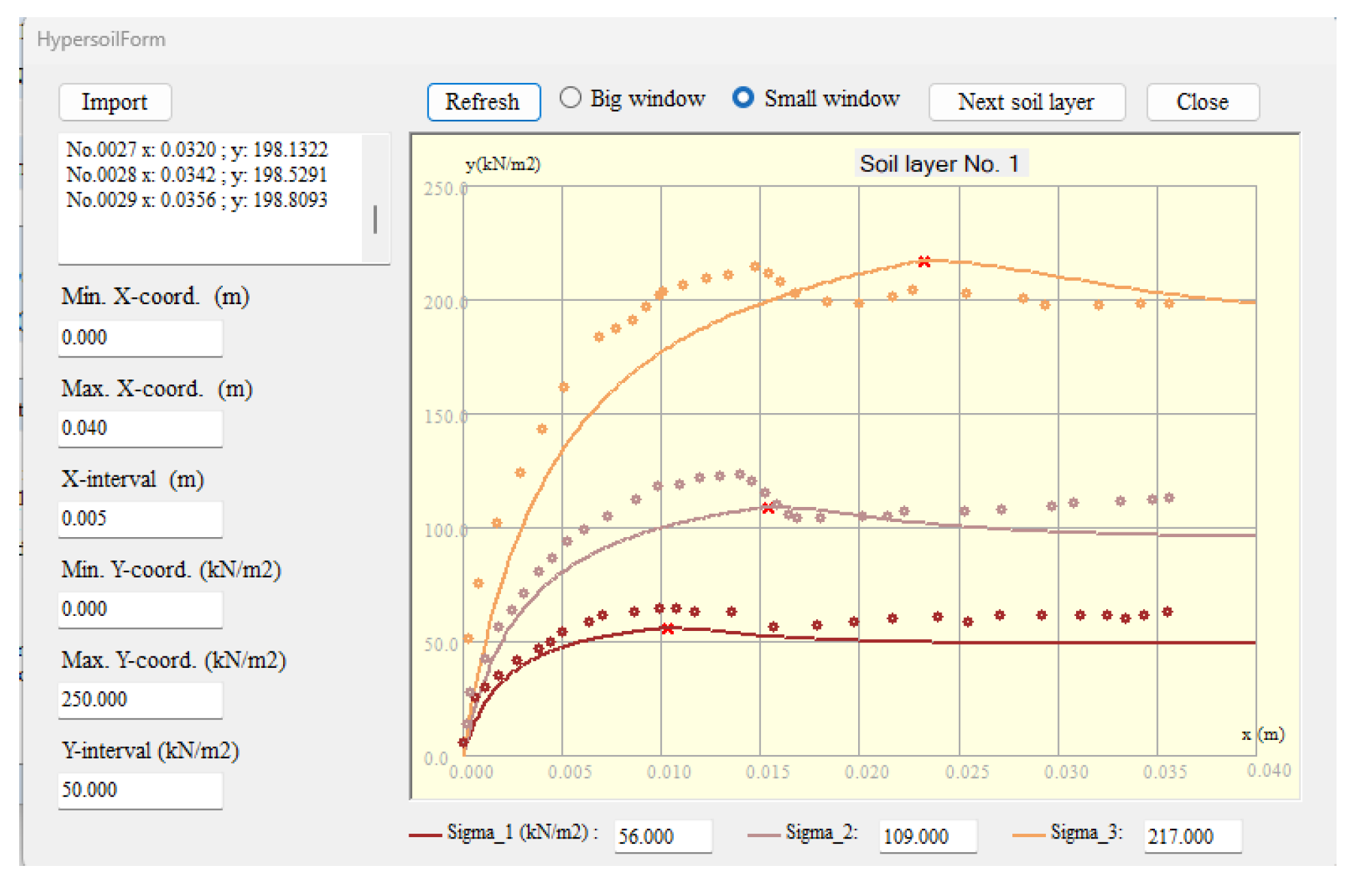
Figure 8 presents an example of the stress–displacement curves visualized with integrated pre-peak and post-peak parameters (ϕpeak= 45°, φᵣₑₛ = 41° , Δᵣ/Δf = 5.0, K = 400, n= 0.4, Rf= 0.83) as summarized in Table 1. For reference, the experimental data reported in [14] from direct shear tests on dense, remolded Chi-Chi sand—classified as SW-SM under the Unified Soil Classification System (USCS)—are also included.
Figure 9 illustrates the visualized hyperbolic pullout curves for reinforcement ( cs-r= 0, ϕs-r= 40°, Ttie-break= 30 kN/m, Kₜ = 10, nₜ= 0.1, and Rₜ= 0.7). For comparison, experimental pullout data for woven geogrids embedded in recycled construction material classified as SM (USCS), as reported in [15], are also shown. It is observed that the theoretical curves exhibit a stronger dependence on confining pressure than the experimental results, likely because the tests were conducted under relatively low confining pressures (10 and 25 kPa), where material uncertainties and measurement errors tend to have relatively large effects.
2.9. FFDM Displacement Analysis
In the Type-4 (multi-wedge) FFDM analysis implemented in SLOPE-ffdm 2.0, a total of 5,389 trial-and-error facing surfaces is employed to identify critical failure mechanisms characterized by the minimum safety factor (Fs) and the maximum vertical displacement at the slope crest (d₀), for a specified pseudo-static seismic coefficient kh (= HPGA/g; g: gravitational acceleration). Figure 10 presents the initial configuration of the multi-wedge analysis, including the trial-and-error search grids for wedge points 1, 2, and 3. In this example, wedge point 3 is fixed at the heel of the rigid facing panel. Once the analysis begins, trial-and-error facing surfaces are systematically generated by connecting all grid combinations, as illustrated in Figure 11. Upon completion of the search, the resulting critical failure mechanisms are displayed in Figure 12. The corresponding failure modes of the reinforcing layers associated with the critical failure surface are also shown in Figure 12, where the symbol “×” denotes tie-break failure and “→” denotes pullout failure.
3. Results
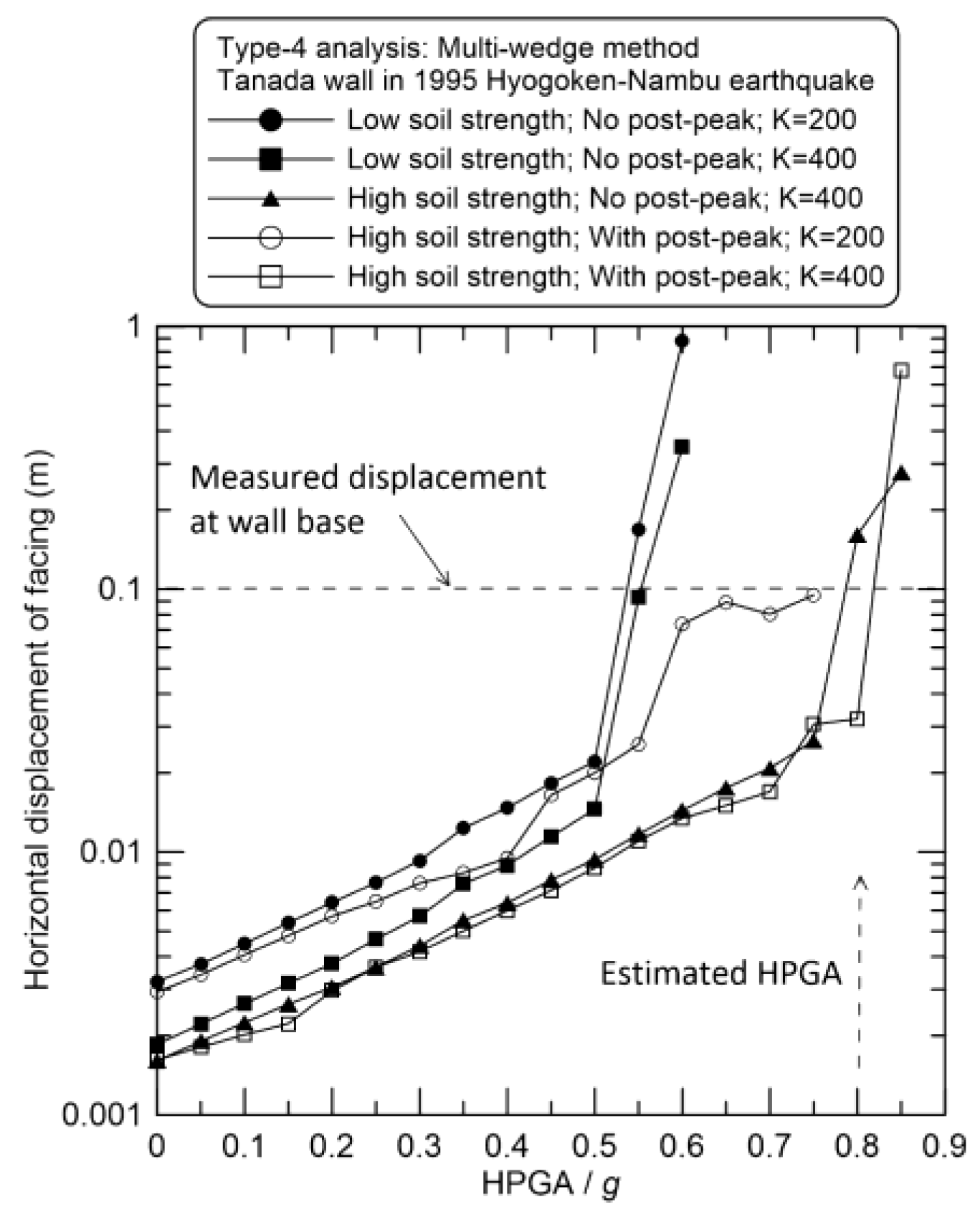
Figure 12 shows the analytical result of FFDM analysis using the multiwedge method (or Type-4 analysis). In this figure, “Low” and “High” soil strength refer to ϕ= 40˚ and 45˚, respectively, listed in Table 1. Every data point in the figure represents a critical (or maximum) value of facing displacement found in 5,389 trial-and-error multiwedge searches. All curves exhibit consistent response to the increase of input HPGA/g in the range of 0.0 - 0.85. In the case ϕ= 40˚ and hyperbolic soil behavior, the response curves exhibit rapid increases in facing displacement at HPGA ≈ 0.5g. When the post-peak model is considered in the analysis, the response curves show a clear tendency toward failure state at HPGA/g ≈ 0.7 - 0.8. In general, the curves with K= 400 and high soil strengtheffectively simulate the observed seismic displacement of the Tanada wall, regardless of the incorporation of post-peak strength. The analysis with a post-peak model verifies not only the earthquake-resisting capacity of the Tanada wall but also the capability of SLOPE-ffdm 2.0 in calculating seismic displacements of geosynthetic-reinforced soil retaining walls. It is also noted that the calculated slope displacements span a wide range between 10⁻³ to 10⁻¹ m, reflecting their engineering significance and accuracy of the computational scheme of the computer program.
To compare the effectiveness of the FFDM with hybrid Newmark-type methods, conventional limit-equilibrium slope stability analyses were conducted to obtain Fs–kh curves for ϕ = 40˚ and ϕ = 45˚, using soil, reinforcement, and facing parameters consistent with those adopted in the displacement analyses. The resulting critical horizontal seismic coefficients are khc = 0.367 and khc = 0.528 for ϕ = 40˚ and ϕ = 45˚, respectively. The value khc = 0.367 agrees well with the lower-bound regression relationship reported in reference [16]. Regression equations relating khc to seismic displacement for GRS-FHR systems subjected to strong ground motions—such as the El Centro, Loma Prieta, Hyogo-ken-Nambu, and Chi-Chi earthquakes—are also provided in reference [16]. Using the regression equation for the Hyogo-ken-Nambu earthquake, the predicted seismic displacements of the GRS-FHR are 132 mm and 30 mm for phi = 40 degrees and phi = 45 degrees, respectively. The displacement of 132 mm for phi = 40 degrees again indicates that, when an operational friction angle of phi = 40 degrees is adopted and an appropriate ground-motion record is selected, a conventional Newmark sliding-block analysis can yield reasonable estimates of seismic displacement for GRS-FHR systems. Nevertheless, this approach has inherent limitations, which will be discussed later.
Figure 12.
Seismic resistance curves for Tanada wall using Type-4 (multi-wedge) analysis
4. Discussion
By integrating soil behavior, reinforcement interaction, and seismic demand within a unified computational platform, the FFDM provides capabilities that extend beyond those of conventional limit-equilibrium methods (LEM). Advantages and limitations of the LEM-based Newmark's and the pseudo-static-based FFDM approaches are:
1. Direct incorporation of peak strength and post-peak degradation: The FFDM explicitly accounts for both peak soil strength and its post-peak degradation along the slip surface. This eliminates the trial-and-error process traditionally required to estimate “operational” strength parameters, thereby streamlining the evaluation of seismic displacements in soil and reinforced-soil systems.
2. Direct use of peak ground acceleration (HPGA/g): Unlike LEM-based seismic analyses that rely on empirically selected seismic coefficients (kh), the FFDM allows HPGA normalized by gravitational acceleration (g) to be used directly as input. This reduces dependence on empirical assumptions and enables more transparent, physically grounded seismic displacement assessments.
3. Limitations of the Newmark approach in pre-earthquake assessments: In a post-earthquake study, a ground excitation recorded at a nearby seismograph may help, to some extent, in reducing the uncertainty of input ground excitations . By using calibrated soil strengths, the LEM-based Newmark's approach is valid in estimating seismic displacement of GRS-FHR. However, this may not be the case in a pre-earthquake assessment. When a broad spectrum of potential ground motions is considered, the predicted seismic displacements may span an excessively wide range. Such variability can obscure the true seismic response of the system and hinder sound engineering judgment. As reported in [16], for a geosynthetic-reinforced soil wall with a non-detectable wall displacement during the 1999 Chi-Chi earthquake, the use of LEM-based Newmark's approach rendered khc= 0.247- 0.278 and δh= 34- 311 mm based on various regression curves for normalized δh vs. khc / km (km= HPGA/ g) relationships reported in [17,18].
4. Contrasting complexity in soil parameters and ground-motion inputs: The LEM-based Newmark approach employs simplified soil strength parameters (primarily cohesion c and ϕ), yet requires ground-motion inputs of considerable complexity, including period characteristics, maximum velocity, and HPGA. In contrast, the FFDM approach incorporates a richer set of soil deformation-related parameters (c, ϕ, K, n, Rf) while using a simplified ground-motion input in which HPGA is the primary concern. This inversion of complexity highlights the more mechanistic nature of the FFDM framework.
5. Capability for back-analysis and parameter calibration: A major advantage of the FFDM is its ability to perform back-analysis to derive soil deformation-related parameters (c, ϕ, K, n, Rf) from small-to-medium earthquake events (for example, HPGA = 0.35 g) in which the retaining structure experiences only minor damage (such as 10 mm of wall displacement). As illustrated in Figure 12, calibrated soil parameters can be inferred from the displacement versus HPGA/g curves. These calibrated parameters can then be used to predict wall displacements under more intense ground shaking. The conventional LEM-based Newmark approach does not offer this capability, as its inherent uncertainties the uncertainties typically exceed several tens of millimeters (that is, on the order of 10⁻² m), making reliable back-analysis impractical.
5. Conclusions
This study, implemented through the SLOPE-ffdm 2.0 program, establishes a displacement-based framework for evaluating the seismic performance of geosynthetic-reinforced slopes using the Force-Equilibrium Finite Displacement Method (FFDM). A performance-based re-evaluation of the Tanada Wall, which experienced intense shaking during the 1995 Hyogoken-Nambu earthquake (ML = 7.2), further validates the effectiveness of the FFDM. The results show that using seismic coefficients derived directly from peak ground acceleration—rather than scaled or empirically adjusted values—eliminates a major source of uncertainty inherent in conventional LEM-based seismic stability analyses. The FFDM also produced realistic and reliable seismic-resistance curves using soil parameters within practically acceptable ranges.
Overall, the study demonstrates that the FFDM, as implemented in SLOPE-ffdm 2.0, provides a robust and practical framework for performance-based seismic evaluation of geosynthetic-reinforced slopes and walls with rigid facings. Its ability to integrate soil behavior, reinforcement interaction, and seismic demand in a displacement-based manner represents a significant advancement over traditional methods and offers a valuable tool for modern geotechnical engineering practice.
This study also highlights key differences between the FFDM and the conventional LEM-based Newmark sliding-block method. The Newmark approach relies on simplified soil strength parameters while requiring consideration of widely varying ground-motion characteristics, which can lead to large variability in predicted seismic displacements. In contrast, the FFDM incorporates a richer set of soil deformation-related parameters while using a simplified ground-shaking input (HPGA), resulting in more transparent and physically grounded predictions.
A major advantage of the FFDM is its capability for back-analysis. For structures that experience only small displacements (for example, on the order of 10⁻³ m) during a medium-scale earthquake, the FFDM can be used to back-calculate soil strength and deformation parameters. These calibrated parameters can then be applied to predict the potential response of the structure under more severe ground shaking. The conventional LEM-based Newmark method does not offer this capability, as its inherent uncertainties typically exceed several tens of millimeters, making reliable back-analysis impractical.
References
- Newmark, N.M. Effects of earthquakes on dams and embankments. Geotechnique 1965, 15, 139–160. [Google Scholar] [CrossRef]
- Huang, C.-C. Developing a new slice method for slope displacement analyses. Engineering Geology 2013, 157, 39–47. [Google Scholar] [CrossRef]
- Huang, C.-C. Force equilibrium-based finite displacement analyses for reinforced slopes: Formulation and verification. Geotextiles and Geomembranes 2014, 42, 394–404. [Google Scholar] [CrossRef]
- Huang, C.-C. Back-calculating strength parameters and predicting displacements of deep-seated sliding surface comprising weathered rocks. Int. J. of Rock Mechanics and Mining Sciences 2016, 88, 98–104. [Google Scholar] [CrossRef]
- Lo, C.-L.; Huang, C.-C. Groundwater-table-induced slope displacement analyses using different failure criteria. Transportation Geotechnics 2021, 26, 100444. [Google Scholar] [CrossRef]
- Lo, C.-L.; Huang, C.-C. Displacement analyses for a natural slope considering post-peak strength of soils. GeoHazards 2021, 2, 41–62. [Google Scholar] [CrossRef]
- Huang, C.-C. SLOPE-ffdm 2.0: Computer programs for slope stability and displacement analyses using Force-equilibrium-based Finite Displacement Method (FFDM), 2025. Available online: https://slope.it.com.
- Duncan, J.M.; Chang, C.Y. Nonlinear analysis of stress and strain in soils. J. Soil Mechanics and Foundation Division, ASCE 1970, 96(SM5), 1629–1653. [Google Scholar] [CrossRef]
- Huang, C.-C.; Chou, L.H.; Tatsuoka, F. Seismic displacements of geosynthetic-reinforced soil modular block walls. Geosynthetics International 2003, 10(1), 2–23. [Google Scholar] [CrossRef]
- Lawrence, J. D. Witch of Agnesi. In A Catalog of Special Plane Curves; Dover Publications: New York, USA, 1972; pp. 20–23. [Google Scholar]
- Atkinson, J.H. An introduction to the mechanics of soils and foundations; McGraw-Hill: Berkshire, England; McGraw-Hill: London, 1993; pp. 215–239. [Google Scholar]
- Tatsuoka, F.; Koseki, J.; Tateyama, M.; Munaf, Y.; Horii, K. Seismic stability against high seismic loads of geosynthetic-reinforced soil retaining structures. Keynote Lecture, 6th Int. Conf. on Geosynthetics, Atlanta, USA, 1998; pp. 103–142. [Google Scholar]
- Huang, C.-C.; Wang, W.-C. Seismic displacement of a geosynthetic-reinforced wall in the 1995 Hyogo-Ken Nambu earthquake. Soils and Foundations 2005, 45(5), 1–10. [Google Scholar] [CrossRef] [PubMed]
- Chiang, Y.-J. Analyses for rainfall-induced slope displacements taking into account various displacement fields and failure criteria. Master thesis, (in Chinese). National Cheng Kung University, Tainan, Taiwan, July 2017. [Google Scholar]
- Vieira, C.; Pereira, P.M. Influence of the geosynthetic type and compaction conditions on the pullout behaviour of geosynthetics embedded in recycled construction and demolition materials. Sustainability 2022, 14, 12070. [Google Scholar] [CrossRef]
- Huang, C.-C.; Wu, S.-H. Simplified approach for assessing seismic displacments of soil-retaining walls. Part Ⅱ: Geosynthetic-reinforced walls with rigid panel facing. Geosynthetics International 2007, 14(5), 264–276. [Google Scholar] [CrossRef]
- Whitman, R.V.; Liao, S. Miscellaneous Paper GL-85-1; Seismic design of gravity retaining walls. Department of the Army, US Army Corps of engineers: Washington, DC, 1985.
- Cai, Z.; Bathurst, R.J. Deterministic sliding block methods for estimating seismic displacements of earth structures. Soil dynamics and Earthquake Engineering 1996, 15(4), 255–268. [Google Scholar] [CrossRef]
Figure 1.
A hyperbolic normalized stress and shear displacement relationship.
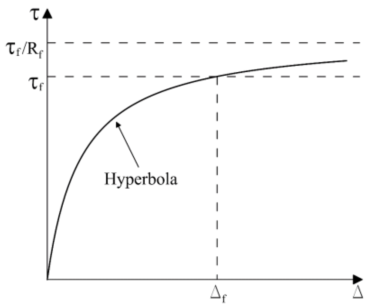
Figure 2.
The multi-wedge failure mechanism.
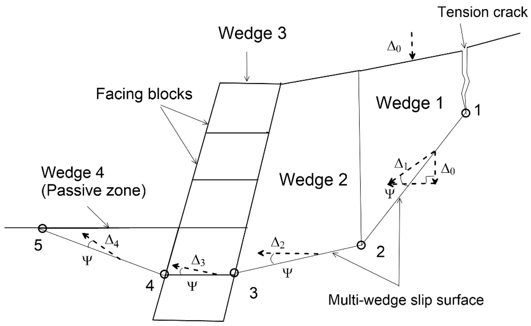
Figure 3.
Force equilibrium for a generalized wedge.
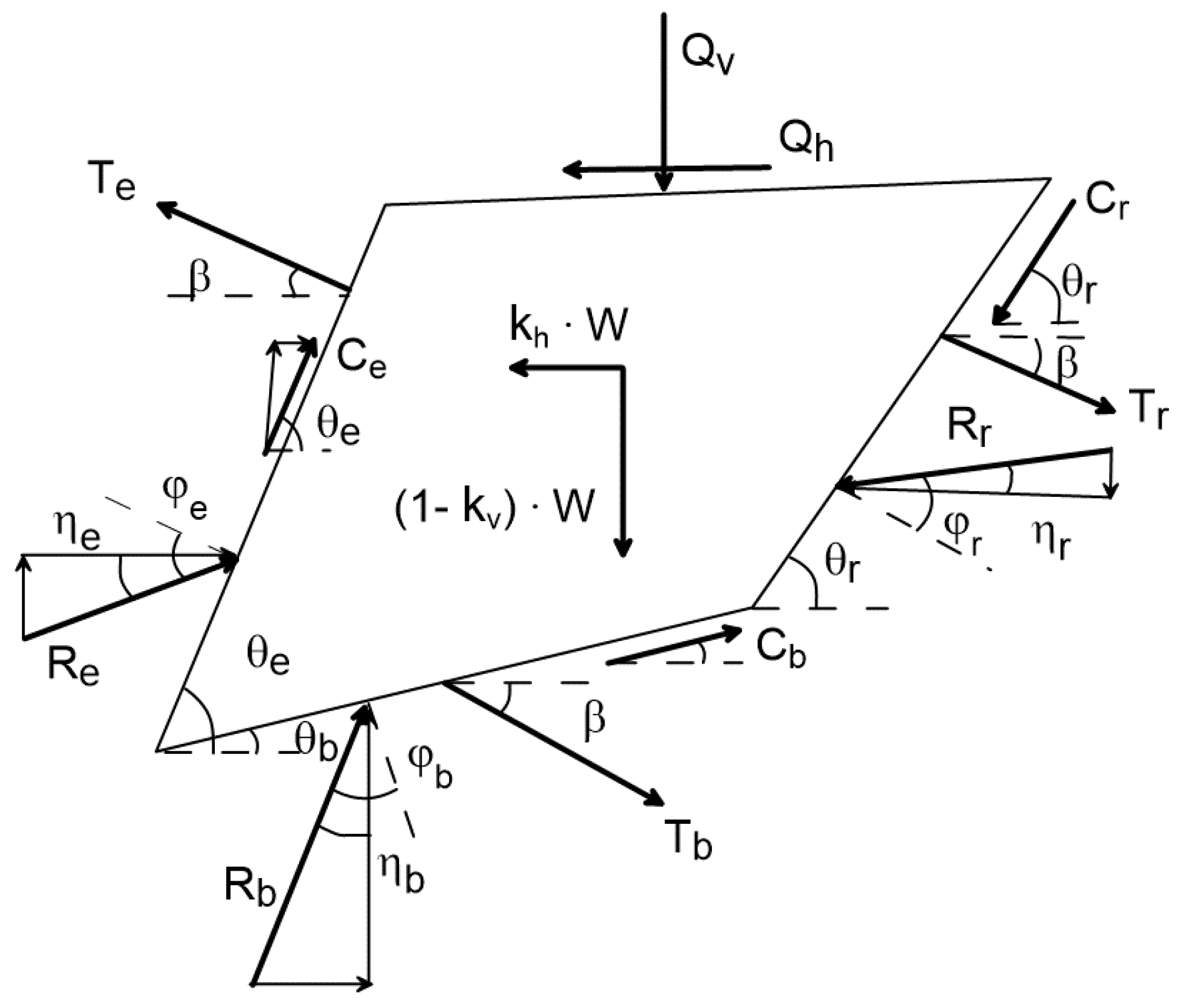
Figure 5.
Displacement compatibility of adjacent soil blocks.
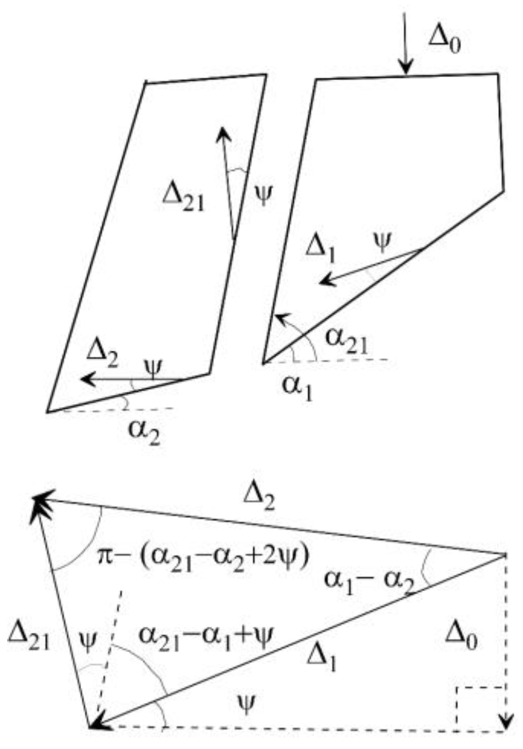
Figure 6.
Schematic stress path in response to seismic-induced stress changes.
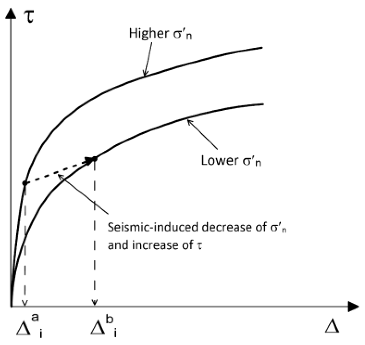
Figure 9.
Stress-displacement curves for reinforcement pullout in the displacement analyses.
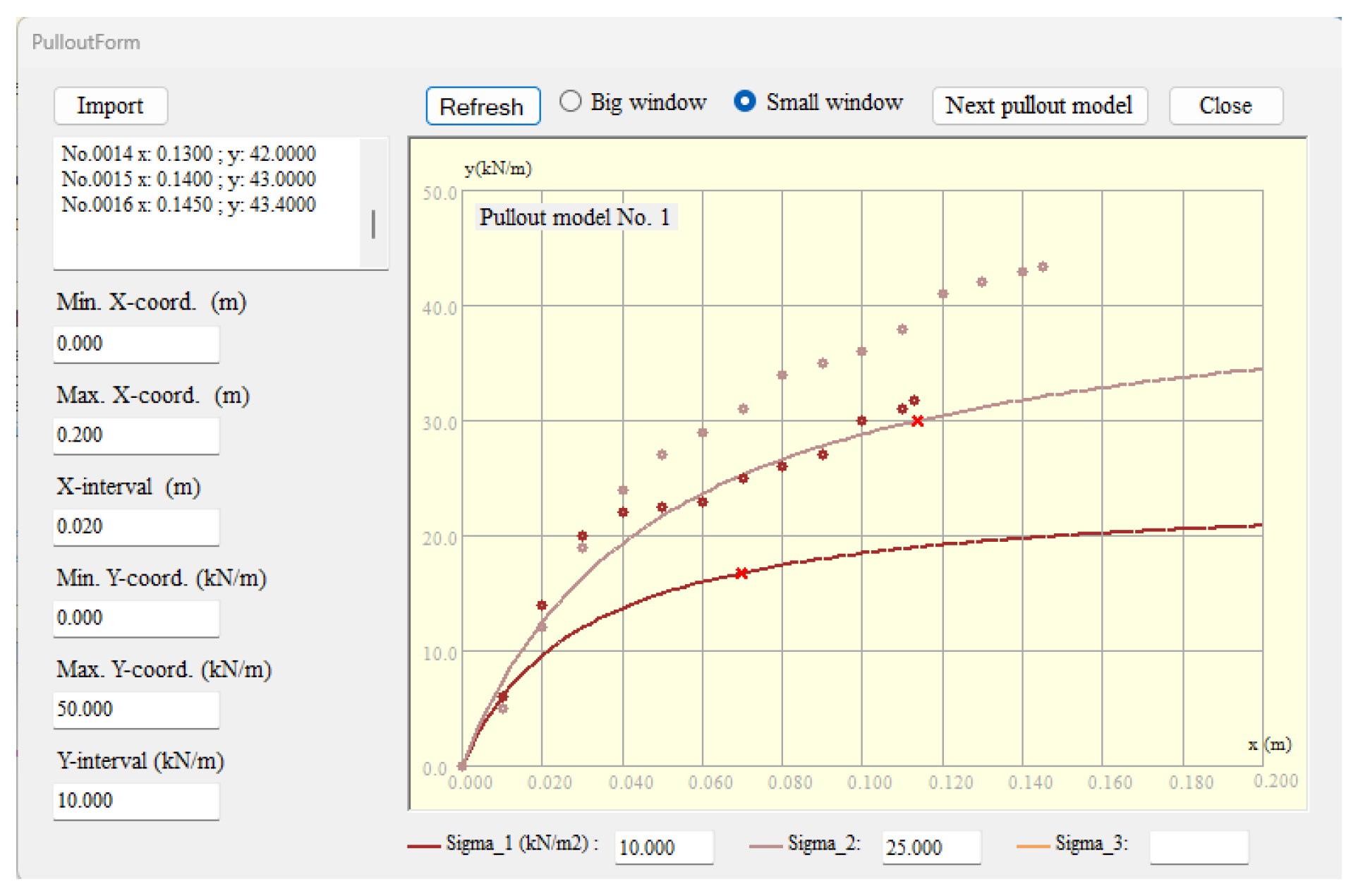
Figure 10.
Initial configuration for the multi-wedge analysis in SLOPE-ffdm 2.0.
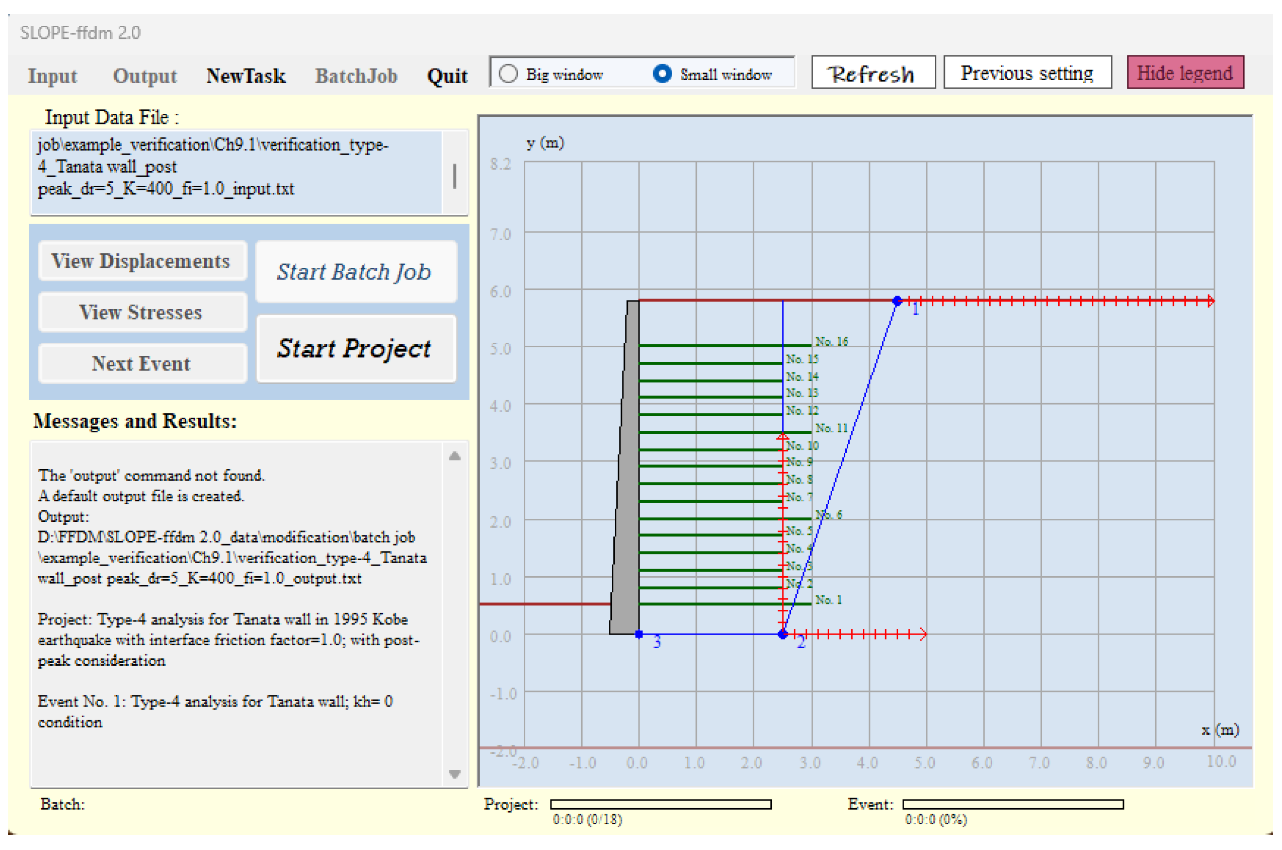
Figure 11.
Searching for the critical failure mechanism using a trial-and-error procedure.
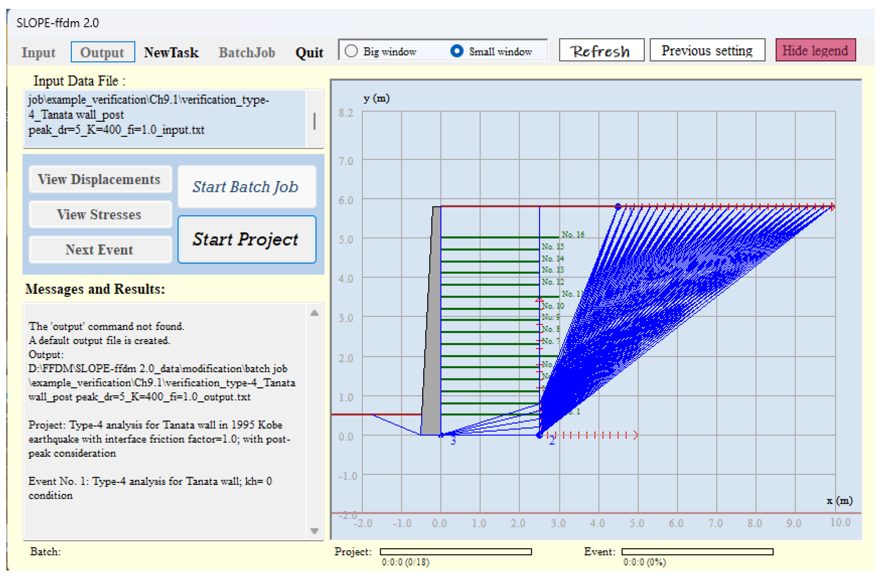
Figure 12.
Critical failure mechanisms identified from the limit-equilibrium and displacement analyses, characterized by the minimum Fs and maximum d0 (vertical crest settlement).
Figure 12.
Critical failure mechanisms identified from the limit-equilibrium and displacement analyses, characterized by the minimum Fs and maximum d0 (vertical crest settlement).
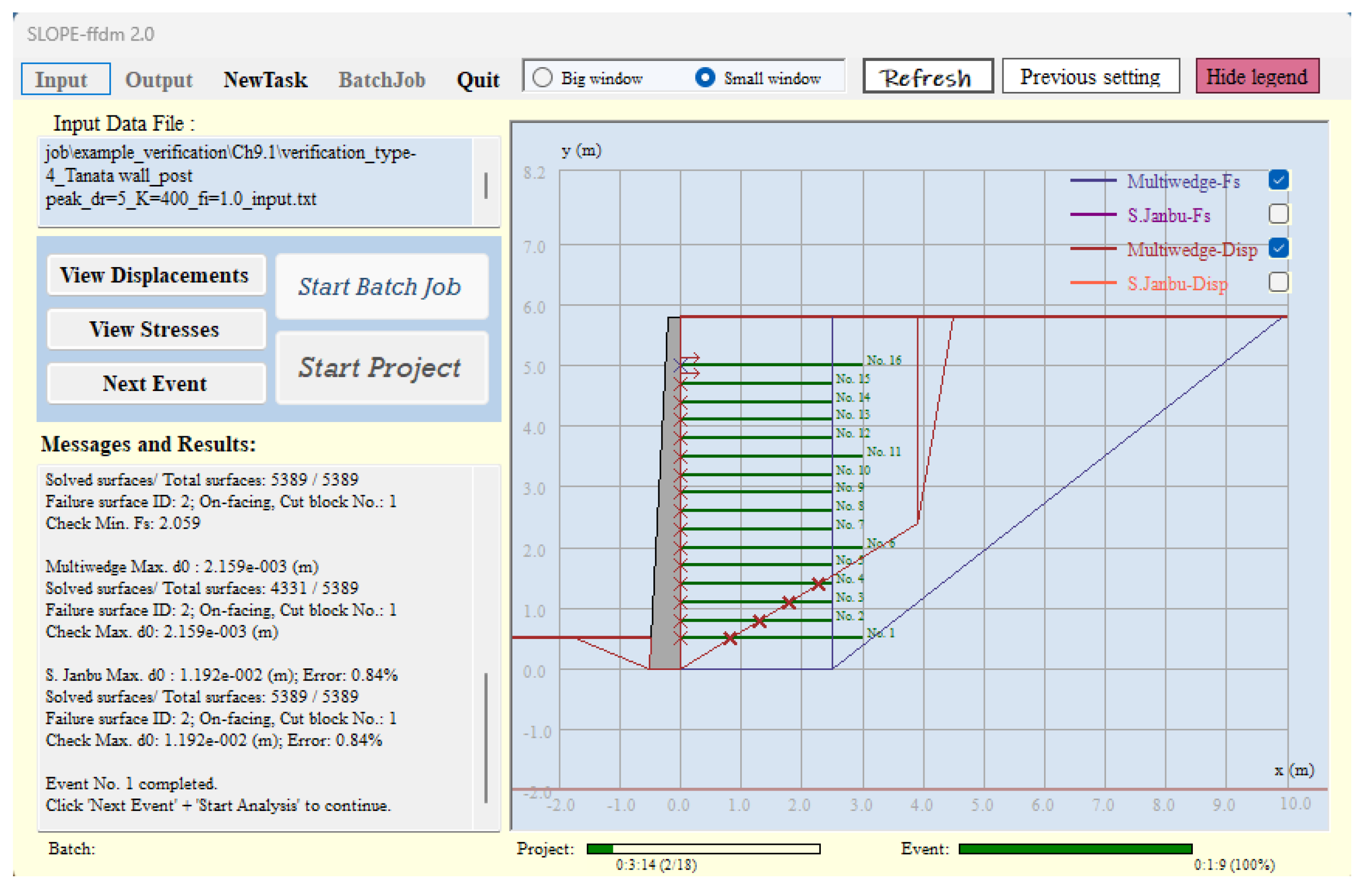

Table 1.
Material properties used in the FFDM analysis for Tanada wall.
|
Soil Hyperbolic model |
Reinforcement Hyperbolic pullout model |
Facing-related strength parameters |
|||
| c | 0 kPa | cs-r | 0 | cb-r | - |
| ϕ | 40° | ϕs-r | 40° | ϕb-r | - |
| K | 200, 400 | Kt | 10 | Tconnect | 30 kN/m |
| n | 0.4 | nt | 0.1 | cback | 0 |
| Rf | 0.83 | Rt | 0.7 | ϕback | 30° |
| Ψ | 5° | Ttie-break | 30 kN/m | cbase | 0 |
| ϕbase | 40° | ||||
| Post-peak model | Post-peak model | Post-peak model | |||
| cpeak | 0 |
Not available |
Not available |
||
| ϕpeak | 45° | ||||
| cres | 0 | ||||
| ϕres | 41° | ||||
| Δr/Δf | 5.0 | ||||
*cs-r, ϕs-r: adhesion and friction angle, respectively, at soil-reinforcement interface. *cb-r, ϕb-r: adhesion and friction angle, respectively, at facing block-reinforcement interface. In the case of rigid panel facing, these values are not required. *cback, ϕback: adhesion and friction angle, respectively, at the back-face of facing. *cbase, ϕbase: adhesion and friction angle, respectively, at the base of facing. *Ttie-break: tie-break of reinforcement. In the FFDM displacement analysis, this value can be different from the design tensile strength of reinforcement (Tallowable) used in the LEM analysis. *Tconnect: connecting force at facing-soil interface. This input is exclusively for the case of rigid panel facing which is equal to Ttie-break in this case study of the Tanada wall.
Disclaimer/Publisher’s Note: The statements, opinions and data contained in all publications are solely those of the individual author(s) and contributor(s) and not of MDPI and/or the editor(s). MDPI and/or the editor(s) disclaim responsibility for any injury to people or property resulting from any ideas, methods, instructions or products referred to in the content. |
© 2025 by the authors. Licensee MDPI, Basel, Switzerland. This article is an open access article distributed under the terms and conditions of the Creative Commons Attribution (CC BY) license (http://creativecommons.org/licenses/by/4.0/).
Copyright: This open access article is published under a Creative Commons CC BY 4.0 license, which permit the free download, distribution, and reuse, provided that the author and preprint are cited in any reuse.


