
Submitted:
12 September 2025
Posted:
15 September 2025
You are already at the latest version
Abstract
The dynamic loads affecting earth retaining structures may increase in seismically active regions. Therefore, studying the soil-structure interaction between the soil, shoring systems, and adjacent structures is crucial. However, there is limited research on this important topic. This study analyzes the seismic performance of a deep-braced excavation and a nearby 10-story building in sandy soil formation. Sandy soil is modeled using the Hardening Soil model with small-strain stiffness (HS-small) using PLAXIS 2D software. The numerical model is validated against measured field data from a real case study of a deep-braced excavation in the central district of Kaohsiung City, adjacent to the O7 Station on the Orange Line of the Kaohsiung MRT system in Taiwan. After model validation, parametric study is conducted to investigate the impact of the foundation level of the building adjacent to the excavation on both the seismic behavior of the shoring system and the structure itself, using the Loma-Prieta (1989) earthquake record. The parametric study is further extended to assess the responses of the shoring system and the adjacent structure under the influence of the earthquake records of Loma Prieta (1989), Northridge (1994), and El Centro (1940). Analysis results show that the maximum lateral displacement of the diaphragm wall occurred at its top in all studied cases. The maximum bending moment in the retaining structure increased by more than three times of that calculated in the dynamic analysis compared to the static analysis. In contrast, the dynamic shear force is more than 2.85 times greater than the static one. In addition, the dynamic axial force in the 1st and 2nd struts increased by 1.38 and 3.17 times, respectively, compared to the static forces. Results also reveal that large differences in behavior of the shoring system and the adjacent structure are noticed between the used different earthquake records.
Keywords:
deep excavation
; seismic analysis
; soil-structure interaction (SSI)
; numerical analysis
; PLAXIS-2D
1. Introduction
Growing population and urban activities within large cities call for underground space to install urban services, transportation infrastructure, parking areas, or other engineering works that call for deep vertical excavations near existing buildings. Retaining structures are essential to prevent large and unsafe soil displacement in the areas around excavation. These retaining structures are constructed and supported at different levels by horizontal struts and/or ground anchors preserving excavation sides and limiting damage to the surrounding structures and utilities.
Braced excavations induce significant changes in stress and strain fields of the soil around them, resulting in permanent displacements to adjacent structures and infrastructures and potentially causing severe damage (El Sawwaf & Nazir, 2012; Lam et al., 2014; Long, 2001; Moormann, 2004a; Ou et al., 1993) in some cases. As the excavation goes deeper, the lateral deflections of the retaining structures need to be controlled to avoid damage to adjacent structures (Boscardin & Cording, 1992; Huynh et al., 2021). Most previous studies have focused on analyzing the behavior of deep excavations under static conditions, utilizing distinct methodologies. Empirical and semi-empirical approaches are commonly used, based on extensive databases of excavation projects from various locations worldwide (Hsieh & Ou, 1998a; Kung et al., 2007; Liu et al., 2005; Long, 2001; Moormann, 2004b; Wang et al., 2010.). Additionally, numerical methods have been extensively employed to investigate various parameters affecting deep excavations and surrounding structures, including soil elasticity, creep, and the soil-wall interface (Arai et al., 2008; Bahrami et al., 2018; Bose & Som, 1998; Chowdhury et al., 2013, 2017; Faheem et al., 2004; Hsiung, 2009; Kung et al., 2007; Liu et al., 2005; Orazalin et al., 2015; Ou et al., 1996; Ou et al., 2013; Ou & Hsieh, 2011; Yoo & Lee, 2008; Zdravkovic et al., 2011). Laboratory model tests are implemented to investigate the static behavior of braced excavation (Chowdhury et al., 2016).
However, limited studies have been performed on braced retaining structures under seismic conditions. Numerical analyses are performed on the braced retaining walls by (Callisto et al., 2008). It is found that as seismic waves propagate through the soil, a quick mobilization of shear stresses in the soil adjacent to the propped cantilever wall is noticed. Therefore, a significant increase in the wall lateral displacement and bending moment is noticed, as well as an increase in the struts axial forces as compared to static conditions. Callisto & Soccodato, (2010) carried out numerical time history analysis applying two earthquake time histories on an embedded cantilever retaining walls in dry, coarse-grained soil using FLAC 2D software. Results pointed out that the seismic resistance to a retaining wall’s permanent rigid body movement could be expressed in terms of critical horizontal acceleration. This critical acceleration is calculated based on limit equilibrium analysis by an iterative method. A significant bending moment increase during earthquakes is also observed due to the instantaneous contact-stress redistribution.
Konai et al., (2018) investigated the behavior of single level of struts of braced excavations in dry sand under seismic conditions through shaking table tests and numerical models. The strut force, lateral displacement, and bending moment are compared from tests and numerical models, using sinusoidal motions to simulate seismic loading. The findings showed that wall stiffness has a greater influence on wall deflection and bending moments than on strut forces under seismic conditions.
Experimental studies have also conducted to investigate the behavior of different types of retaining structures under seismic conditions (Ling et al., 2009; Ling, Liu, et al., 2005; Ling, Mohri, et al., 2005; Madabhushi & Zeng, 2007; Mikola & Sitar, 2013; Tufenkjian & Vucetic, 2000).
Bahrami et al., (2019) performed a numerical study on the seismic performance of strutted diaphragm walls in dry sand. Results indicated that structures designed using Peck method performed adequately under static loads. However, under seismic conditions, the bending moments and shear forces on the wall, as well as the axial forces on the strut, increased significantly, exceeding the permissible limits specified in (ACI Committee, 2008) and (ASCE standard ASCE/SEI 7-16, 2017). Castaldo & De Iuliis, (2014) conducted a numerical analysis on the seismic vulnerability of existing buildings affected by adjacent deep excavations. By considering the nonlinear dynamic properties of both soils and structures, it is found that the presence of adjacent excavation significantly increased the ductility demand and inter-story drift of nearby buildings.
Chowdhury et al., (2015) investigated the behavior of a strutted retaining structure under seismic conditions numerically by FLAC-2D. It is observed that wall lateral displacement is the most affected parameter during an earthquake, and the axial force of the struts is the least affected parameter.
The finite difference method in FLAC-2D is used to investigate soil-structure interaction, building-excavation interaction, and fixed-base structure models by (Yeganeh et al., 2015).
This research investigates the performance of deep braced excavations in sand under seismic loads, considering the interaction with adjacent structures. The hardening soil model with small-strain stiffness (HS-small) is employed to simulate the soil’s non-linear and hysteretic behavior in both static and dynamic conditions. Model validation is performed using a well-documented case study of a deep-braced excavation in sandy soil as cited in (Hsiung & Dao, 2014). Following validation, dynamic boundary conditions are applied to the model before imposing seismic loads. The boundary conditions allow for absorbing incident seismic waves and preventing their reflection into the model. Additionally, the mesh size is optimized to ensure smooth propagation of seismic waves through all elements without distortion or numerical errors. This study focused on the response of strutted diaphragm walls and surrounding structure under different earthquake records. The acceleration time histories of Loma-Prieta (1989), Northridge (1994), and El Centro (1940) earthquakes are utilized in this study. Moreover, the foundation level is also investigated under the effect of the Loma-Prieta (1989) earthquake record. The study discusses the diaphragm wall lateral displacements, settlement trough behind the wall, straining actions of the diaphragm wall, axial forces in the struts, and the maximum story displacement of the adjacent structure under static and seismic conditions to evaluate and assess the seismic performance of both the deep braced excavation and the adjacent structure.
2. Numerical Modeling
The static and dynamic behavior of soil is efficiently simulated using plain strain analysis. HS-small strain model which is implemented in PLAXIS-2D based on research of (Benz, 2007b) is used to model soil behavior because of accounting for the stress dependency of stiffness and variation of secant shear stiffness ratio (Gs/Go) with increasing shear strain amplitude (γ). HS-small strain model follows a hyperbolic approximation of the stress-strain curve proposed by Hardin (Hardin & Drnevich, 1972), which is modified later by Santos et.al (Santos & Correia, 2001) given as:
where, τ is shear stress, and Gs is secant shear modulus corresponding to shear strain (γ). The γ0.7 is the shear strain at which Gs is reduced to 70% of Go. In HS-small model, the stress dependency of the shear modulus G0 is considered with the power law which resembles the ones used for the other stiffness parameters as indicated in Eq.2. The threshold shear strain γ0.7 is taken independently of the mean stress as following:
Moreover, the model uses strength parameters of Mohr-Coulomb (cohesion c, friction ϕ) as well as soil stiffness is defined by three input values: E50 (secant stiffness modulus at 50% deviatoric stress (qf)) given by Eq.3, Eoed (1D oedometer loading modulus), and Eur (unloading-reloading modulus).
where is the secant modulus corresponding to the reference confining pressure, pref (equal to 100 kN/m2). The is the minor principal stress. Here, m accounts for stress dependency. According to (Benz, 2007a) in this study it is taken to be equal 0.50. The default values of Eoed = , and Eur = 3 as proposed by (Brinkgreve et al., 2006; Obrzud, 2010).
A small Rayleigh damping of 2% is used in this study during the dynamic analysis to remove the heigh-frequency noise resulting from the numerical integration. In finite element formulations, the damping is often formulated as a function of the mass and stiffness and is defined as proposed by (Chopra, 2007; Hughes, 2003; Zienkiewicz & R.L. Taylor, 1991) :
where [M] is the mass matrix; [K] is the stiffness matrix; and α and β are
The Rayleigh damping coefficients and given by:
Where ζ is the damping ratio and it is 2% in this study; ω1 and ω2 are considered the target angular frequencies corresponding to the target circular frequencies f1, f2, respectively.
2.1. Meshing Considerations
The response of both linear and nonlinear finite element models is influenced by discretization of real models. During dynamic analysis the maximum dimension of any element should be limited to one-eighth to one-fifth of the shortest wavelength considered in the analysis as suggested by the researchers (Kuhlemeyer & Lysmer, 1973; Lysmer et al., 1975). In this research, 15-node triangular soil elements are used to model soil continuum. The dimension of the elements is controlled, and the local mesh refinement is implemented to achieve an appropriate value for the average length of the element side to the propagated seismic waves without numerical errors.
2.2. Boundary Conditions
For static analysis the movement of lateral boundaries is restrained horizontally, while movements for the bottom boundary of the model are restrained horizontally and vertically. During the dynamic analysis a repeatable tied degree of freedom boundary condition which is proposed by (Zienkiewicz et al., 1989) is utilized to simulate the lateral boundaries of the model to tie the nodes on the same elevation to have the same displacements. On the other hand, a compliant base boundary condition is applied at the bottom of the model to consider the absorption and application of the dynamic load as proposed by Joyner and Chen (Joyner & Chen, 1975).
3. Verification of Case Study on Deep Excavation in Sand (Hsiung & Dao, 2014)
A real case study of a deep-braced excavation in Kaohsiung, Taiwan presented by (Hsiung & Dao, 2014), as shown in Figure 1, is utilized to validate the numerical model before dynamic analysis to assess the model accuracy in capturing the behavior of real braced-excavation. The excavation dimensions are 70 m length and 20 m width, with 16.8 m depth. A 0.90 m diaphragm wall is used as a retaining structure, supported by four levels of steel struts spaced 5.50 m apart horizontally. The excavation is executed in medium dense to dense silty sand soil with bands of low plasticity clay (CL). Additionally, before excavation the groundwater level is approximately 2.0 m below the ground surface as shown in Figure 2.
The measured lateral displacement of the diaphragm wall and the settlement of the ground surface are shown in Figure 3.
The case study is numerically back analyzed using PLAXIS-2D FE software developed by (Brinkgreve & Vermeer, 2002). Plane-strain FEM model is carried out adopting a 15-node triangular element to model deformations and stresses in soil volume. The Hardening soil with small strain model (HS-small ) is utilized in this study, as recommended by (Hsiung & Dao, 2014), to represent the behavior of the sand layers whereas, the elastic-perfectly plastic Mohr-Coulomb (MC) model is used to describe the behavior of the clay layers. The soil properties are presented in Table 1 and Table 2. The diaphragm wall and steel struts are modelled as linear elastic materials, adopting plate elements for the diaphragm wall and fixed-end anchors for the steel struts. Poisson’s ratio of 0.2 is assigned to both the diaphragm wall and steel struts. The diaphragm wall Young’s modulus is 24.8 × 10⁶, while Young’s modulus of steel struts is taken equal to 2.1 x 10⁵ (MPa). The stiffness of the diaphragm wall and steel struts are decreased by 30% and 40%, respectively, from their nominal values to account for bending moment-induced cracks in the diaphragm wall, repeated use, and improper steel strut installation as suggested by (Ou, 2014) for detailed data about diaphragm wall and steel struts refer to (Hsiung & Dao, 2014).

Table 1.
Soil properties used in the numerical validation model of the sand layers using HS-small model as proposed by (Hsiung & Dao, 2014).
Table 1.
Soil properties used in the numerical validation model of the sand layers using HS-small model as proposed by (Hsiung & Dao, 2014).
| Soil Layer | 2 | 4 | 5 | 6 | 8 | 9 |
| Depth (m) | 2.00-6.50 | 8.0-17.00 | 17.00-23.50 | 23.50-28.50 | 30.5-42.0 | 42.0-60 |
| Soil Type according to USCS | SM | SM | SM | SM | SM | SM |
| SPT (N-Value) | 5-11 | 5-17 | 5-17 | 5-17 | 18-26 | 28-42 |
| γt (kN/m3) | 20.9 | 20.60 | 18.60 | 19.60 | 19.60 | 19.90 |
| Internal friction angle | 32 | 32 | 32 | 33 | 34 | 34 |
| Cohesion, | 0.50 | 0.50 | 0.50 | 0.50 | 0.50 | 0.50 |
| Angle of dilation, Ψ | 2 | 2 | 2 | 3 | 4 | 4 |
| Drained triaxial reference secant stiffness | 9600 | 13200 | 13200 | 13200 | 26400 | 42000 |
| Oedometer primary loading reference tangent stiffness | 9600 | 13200 | 13200 | 13200 | 26400 | 42000 |
| Unloading/reloading reference stiffness | 28800 | 39600 | 39600 | 39600 | 79200 | 126000 |
| Unloading/reloading Poisson’s Ratio‘ur |
0.20 | 0.20 | 0.20 | 0.20 | 0.20 | 0.20 |
Table 1.
Soil properties used in the numerical validation model of the sand layers using HS-small model as proposed by (Hsiung & Dao, 2014), Continued.
Table 1.
Soil properties used in the numerical validation model of the sand layers using HS-small model as proposed by (Hsiung & Dao, 2014), Continued.
| Soil Layer | 2 | 4 | 5 | 6 | 8 | 9 |
| Power for dependency of stiffness on stress level, m | 0.50 | 0.50 | 0.50 | 0.50 | 0.50 | 0.50 |
| Failure ratio, Rf | 0.90 | 0.90 | 0.90 | 0.90 | 0.90 | 0.90 |
| The coefficient of earth Pressure at rest, |
0.47 | 0.47 | 0.47 | 0.46 | 0.44 | 0.44 |
| Reference small strain shear modulus, G0 ref (Kpa) | 69657 | 57153 | 42069 | 39966 | 59204 | 73412 |
| Shear strain at 0.722G0, γ0.7 | 10−4 | 10−4 | 10−4 | 10−4 | 10−4 | 10−4 |
| Analysis Type | Drained | Drained | Drained | Drained | Drained | Drained |
| Rinterface | 0.67 | 0.67 | 0.67 | 0.67 | 0.67 | 0.67 |
Table 2.
Soil properties of the clay layers using the MC-model, as presented in (Hsiung & Dao, 2014):.
Table 2.
Soil properties of the clay layers using the MC-model, as presented in (Hsiung & Dao, 2014):.
| Soil Layer | Depth (m) |
Soil Type |
t (kN/m3) |
Su (kPa) |
Eu (kPa) |
undrained Poisson’s ratio,νu | Analysis Type | Rinterface |
| 1 | 0.0-2.0 | CL | 19.30 | 28 | 14000 | 0.495 | Undrained | 0.67 |
| 3 | 6.5-8.0 | CL | 19.70 | 21 | 10500 | 0.495 | Undrained | 0.67 |
| 7 | 28.0-30.5 | CL | 18.60 | 84 | 42000 | 0.495 | Undrained | 0.67 |
The verification model is extended to a depth of 60 m below the ground surface in accordance with site investigation program. The lateral boundary of the model to the diaphragm wall is taken to be seven times the final excavation depth as suggested by (Khoiri & Ou, 2013) for deep excavations in sands as shown in Figure 4a. Mesh discretization shown in Figure 4b is set to global medium, and local refinement is implemented to increase the accuracy of the analysis.
3.1. Verification Results of the FEM Model
Wall lateral displacements resulting from the finite element simulation at the final stage of the excavation are compared with the measured one from the field data presented in Figure 5. The measured and predicted lateral displacements at the final stage of excavation showed good agreement. This implies that the HS small strain model achieved best prediction of the wall lateral deflections and ground surface settlement in such simulations of these cases, and this is consistent with the findings of the researchers (Hsiung & Dao, 2014; Khoiri & Ou, 2013; Likitlersuang et al., 2013). The ground surface settlement adjacent to the diaphragm wall is also investigated and compared to those of field-measurements, as shown in Figure 6. It is demonstrated that the HS-small strain constitutive soil model predicts the settlement in reasonable agreement with field-measured data, especially beside the diaphragm wall. However, the predicted settlement seems to be larger than the measured ones as the excavation goes deeper to the final level but still the settlement trough has the same pattern as proposed by (Hsieh & Ou, 1998b) for braced excavations.
4. Dynamic Modeling of the Shoring System and Adjacent Structure
This research focuses on a braced excavation with 10.00 meter’ depth that is modeled in a dense sand soil with 60.00 meters deep, overlying bedrock with surrounding structure composed of a basement and nine replicated stories, each with two spans of 5.00 meters. Vertical boundaries at the right and left edges of the model shown in Figure 7 are chosen to be at 7B (where B is the width of excavation) from the left and right walls, respectively. Soil properties used in this study are presented in Table 3. The shoring system and surrounding structure are modeled statically and dynamically using different earthquake records. Static and dynamic behavior is investigated.
In this analysis the diaphragm wall is modeled as linear elastic plate elements with Young’s modulus of 26.00 GPa that is calculated according to ACI -318 and Poisson’s ratio is taken to be equal to 0.20, as well. Rayleigh damping of 5% is considered during seismic analysis.
Two levels of struts with horizontal spacing in the longitudinal direction equal to 5.00 m are used in this study the first level is installed at 2.00 m from the ground surface, and the second one is installed at 6.00 m from the ground surface as recommended by the design guide of (Chowdhury et al., 2013). The struts are simulated using linear elastic node-to-node anchors with axial stiffness 25 x 106 and 50 x 106 kN/m2, respectively.
A reinforced concrete structure composed of two bays each of 5.00 m width with one basement of 3.25 m height and nine typical stories of 3.00 m height each is set adjacent to the shoring system. The equivalent dead and live loads are considered 10 kN/m’/storey. The structural elements are simulated using linear elastic plate elements with axial and flexural stiffness to model columns, walls, beams, and slabs of equivalent thickness of 0.30 m, while the raft foundation has 1.00 m thickness. Interface elements are added to simulate soil-structure interaction between the basement walls, raft and the surrounding soil.
5. PARAMETRIC STUDY
The main objective of this study is to investigate the seismic performance of deep-braced excavations in sand considering the presence of a building adjacent to the excavation to consider the soil-structure interaction. All the parameters studied are summarized in Table 4.
Initially, static analysis is performed considering that the diaphragm wall is wished-in-place and no deformation accumulated from the adjacent wall construction, then the excavation starts to the pre-defined levels up to the final excavation level. After each excavation stage, the bracing system is also installed at the proposed locations. Eventually, dynamic analysis is carried out imposing the seismic loads as a prescribed displacement in the horizontal direction (i.e., Global X-direction) using a dynamic multiplier that represents the time history of the seismic ground motions.
In the dynamic stage of construction, the dynamic boundary conditions, and damping are implemented to the model before running the analysis. The dynamic time intervals are used as the total time of the earthquake record. The time steps are also adjusted to match the number of data points that represent the dynamic multiplier of the ground motion.
5.1. Characteristics of the Input Ground Motions
Acceleration time histories of three well-known earthquakes of Loma-Prieta (1989), Northridge (1994) and El Centro (1940) retrieved from the Pacific Earthquake Engineering Research Center (PEER) (PEER, 2022) are considered and applied on bedrock after the last stage of excavation as shown in Figure 7 through 10 . The main characteristics of the earthquake records are given in Table 5.
Figure 7.
Acceleration time history of the Loma-Prieta (1989) Earthquake of Mw (6.90).
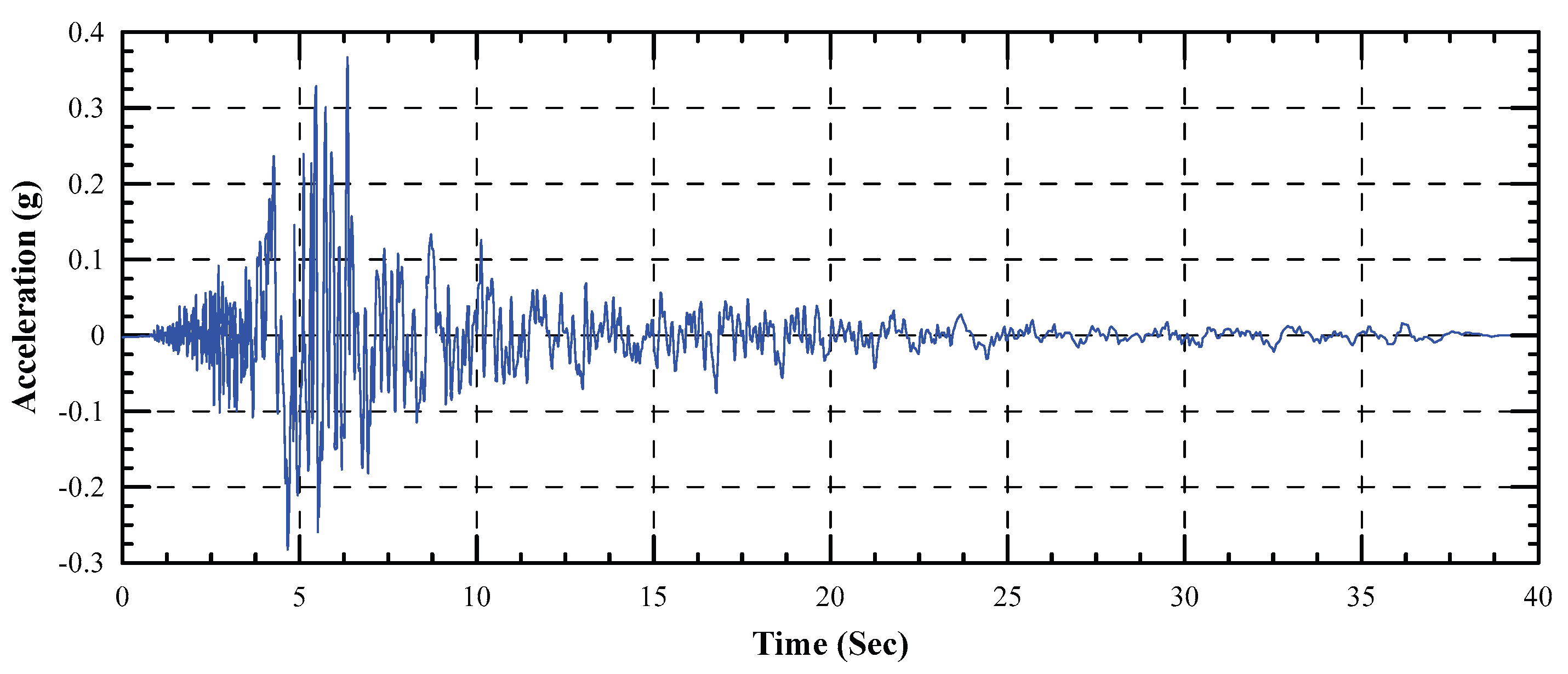
Figure 8.
Acceleration time history of the Northridge (1994) Earthquake of Mw (6.70).
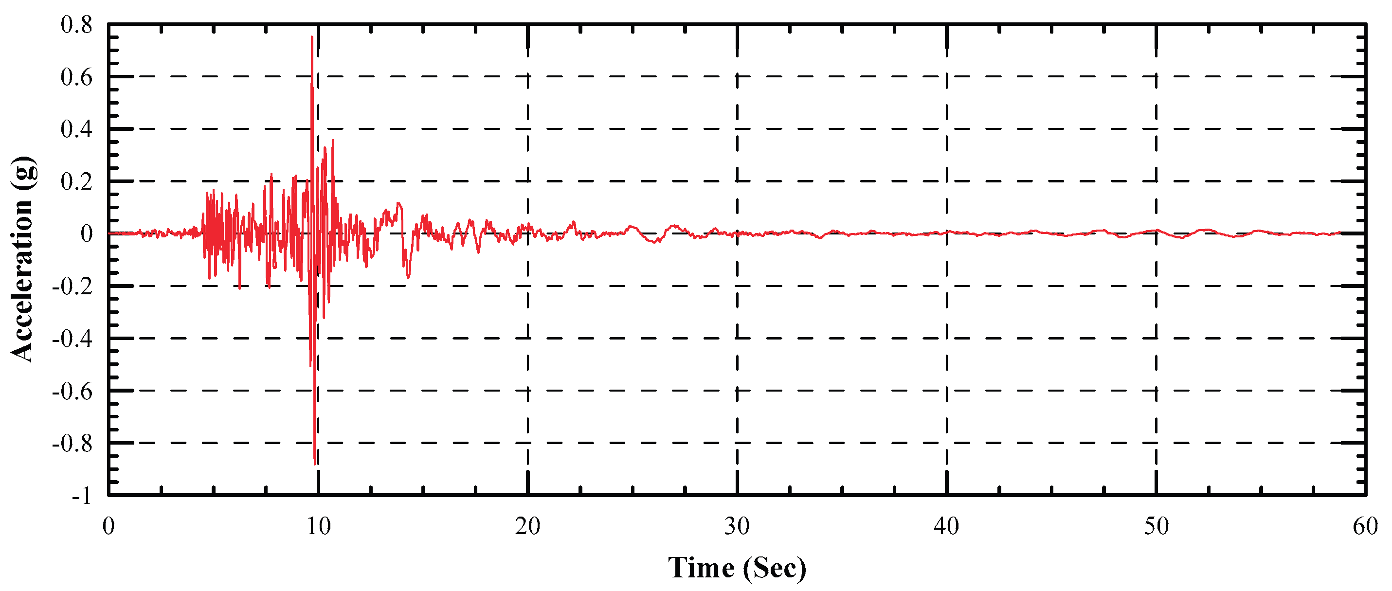
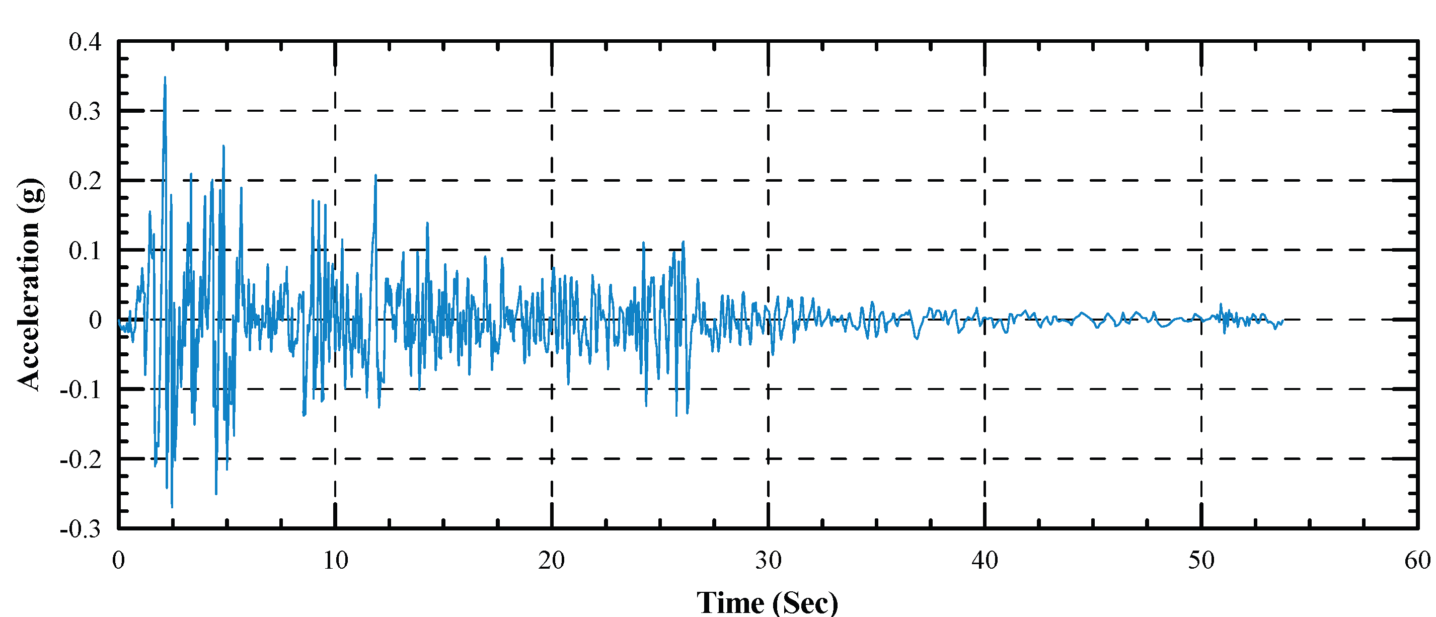
Figure 9.
Acceleration time history of the El-Cento (1940) Earthquake of Mw (6.90).
6. Analysis Results and Discussion
The parametric study aims to assess the shoring system design parameters and the behavior of adjacent structures in static and seismic analyses.
6.1. Effect of Adjacent Structure Foundation Level on Shoring System-Structure Interaction
6.1.1. Displacement-Time History (DTH)
Figure 10 a, b, and c present displacement-time history at the top of the diaphragm wall and the top roof of the adjacent structure, respectively for different foundation levels of the structure adjacent to the shoring system. The free-field ground surface response (point B in Figure 7) for different foundation levels is shown in Figure 10. a, indicates that the response for all foundation levels is the same as original ground motion at the base with time difference of 0.33 sec and maximum amplification ratio of 232%, 209% and 203% for 1.00 m, 3.00 m, and 5.00 m depth, respectively. It is also noticed that permanent lateral displacements of the ground surface in the same direction as the original ground motion of 62.92 mm, 16.71 mm, and 0.56 mm, for depths of 1.00 m, 3.00 m, and 5.00 m, respectively. Results showed that as the building foundation level increased, the permanent displacement of ground surface decreased significantly by 73.40% as the foundation depth increased from 1.00 to 3.00 m and 96.60% as the foundation depth increased from 3.00 to 5.00 m depth.
Figure 10.b, indicates the response of the top of diaphragm wall (Point C in Figure 7) for different foundation levels. Resuls show a time difference of 0.23 sec at the top of diaphragm wall and amplification of the incident waves by 331%, 385%, and 388% for foundation dephs of 1.00, 3.00, and 5.00 m, respectively. The top of diaphragm wall experience a permanent lateral displacement at the end of earthquake of -87.89, -128.03, and -138.55 mm for foundation levels of 1.00, 3.00, and 5.00 m, respectively. The response of the top of diaphragm wall indicates that the wall displacement at the top increased as the structure foundation level increased. As foundation level increased from 1.00 to 3.00 m the permanent displacement increased by 45.70% and increased by 8.20 % as depth increased from 3.00 to 5.00 m. More details about this behavior will be discussed in Section (6-1-3).
Figure 10.c, indicates the response at the top of structure adjacent the shoring system (Point D in Figure 7). Results show that the displacemnt at the top roof increased significantly as the foundation level of the structure increased. The structure undergoes large permanent lateral displacemnts at the top roof at the end of ground shaking. The lateral displacements are amplified by 41.22, 36.37, and 25.80 times as compared to the original ground motion for foundation levels of 1.00, 3.00, and 5.00 m, respectively. The top roof exhibited permanent lateral displacement of -348.32, -406.54, and -446.15 mm at the end of shaking for foundation levels of 1.00, 3.00, and 5.00 m, respectively. As foundation level increased from 1.00 to 3.00 m, the permanent displacement increased by 16.70 % and as the depth increased from 3.00 to 5.00 m, the permanent dispalcement increased by 9.70%.
6.1.2. Settlement Trough beside the Shoring System
Figure 11. a and b, represent the results of settlement trough in static and dynamic cases for different foundation levels of the structure adjacent to shoring system, respectively. The static settlement trough shown in Figure 11.a, shows that as the foundation level of the structure increased, the settlement trough decreased significantly. Moreover, the extent of the settlement trough decreased as the foundation level increased, and for structure foundation level of 1.00 m the settlement trough extended to five times the ultimate excavation depth (5H) until no significant changes are noticed. On the other hand, for foundation levels of 3.00 m and 5.00 m, the settlement trough extended to two times the ultimate excavation depth (2H) until no significant changes are noticed. Results indicate that the structure exposed to differential settlement due to excavation and the differential settlement decreased as the foundation level increased.
On the contrary, the dynamic settlement trough, shown in Figure 11.b, behaves in different manner than the static one. Results indicate that the settlement trough and the differential settlement of the structure increase as the foundation level of the structure increases from 1.00 m to 3.00 m while as the foundation level increased from 3.00 m to 5.00 m, settlement trough and differential settlement decreased once more. The dynamic trough extends to three times the final excavation depth (3H) and beyond this distance no significant changes in the settlement are noticed. Results of the dynamic trough indicate that the ground surface exposed to uniform permanent vertical settlement of about 5.0 cm for all foundation levels.
6.1.3. Lateral Displacement of the Shoring System
Figure 12.a and b investigate the diaphragm wall lateral displacements for different foundation levels of the adjacent structure in both static and dynamic cases, respectively. The static lateral displacements of the diaphragm wall presented in Figure 12.a shows that the lateral displacements decreased significantly as the foundation level of the structure increased. The lateral displacement at the top of diaphragm wall decreased by 60.70% as the foundation level increased from 1.00 m to 3.00 m and decreased by 18.10% as the foundation level increased from 3.00 m to 5.00 m, respectively. However, lateral displacement of the wall in the dynamic case behaves in different ways, as shown in Figure 12.b. In the dynamic analysis, the maximum lateral displacement occurred at top of the diaphragm wall. Moreover, as the structure foundation level increased, the lateral displacement of the wall increased significantly. As the structure foundation level increased from 1.00 m to 3.00 m, the dynamic lateral displacement at the top of the diaphragm wall increased by 47.10%, while as the foundation level increased from 3.00 m to 5.00 m the lateral displacement increased by 9.50%. On the other hand, as the foundation level increased from 3.00 m to 5.00 m the dynamic lateral displacements beyond bottom of excavation level decreased by 8.40%.
Figure 13 presents comparison between the dynamic and static lateral displacements at the top of the diaphragm wall and at the bottom of excavation level for different foundation levels of structure adjacent to the shoring system. The dynamic lateral displacements at the top of wall are 1.15, 4.32, and 5.77 times, as compared to static ones for structure foundation levels of 1.00 m, 3.00 m, and 5.00 m, respectively. Moreover, the dynamic lateral displacement at bottom of excavation level is of 1.43, 3.37, and 4.15 folds, when compared to static ones for structure foundation levels of 1.00 m, 3.00 m, and 5.00 m, respectively.
This significant increase in the dynamic values is attributed to amplification of the seismic waves while being transmitted from the base of model to the ground surface. This behavior implies the vital role of foundation levels of structures in adjacent to deep excavation projects on the behavior of shoring system in dynamic cases. Moreover, modeling the structure adjacent to excavation as a real structure not only as surcharge load is very important and shows the importance of seismic soil structure interaction (SSSI) in complex problems, such as deep excavations.
6.1.4. Staining Actions of Diaphragm Wall and Its Supporting Struts
The foundation level of the structure adjacent to deep excavation affects the straining actions in the diaphragm wall and axial force of the supporting struts, as well. The static and dynamic bending moments along the wall are shown in Figure 14.a and b, respectively. The pattern of the resulting static bending moments of foundation level of 1.00 m is different from other foundation levels of 3.00 m and 5.00 m, especially at the location of the 2nd strut. The bending moment at the location of the 2nd strut decreases as the foundation level increases. The maximum static bending moment occurs at 87.5% H for all foundation levels. It is also noticed that the maximum moment beyond the bottom of excavation level occurred at depths between (15 to 25) % D. On the other hand, the dynamic bending moment distribution shown in Figure 14.b reveals that the maximum bending moment occurs at the location of the 2nd strut.
Furthermore, the static bending moment increased by 37.51% as the foundation level increased from 1.00 m to 3.00 m while, decreased by 11.48 % as the foundation level increased from 3.00 m to 5.00 m. Moreover, the dynamic bending moments decreased by 12.17% as the foundation level increased from 1.00 m to 3.00 m while, increased by 7.96 % as the foundation level increased from 3.00 m to 5.00 m.
Figure 14.c and d, investigate the static and dynamic shearing forces along the diaphragm wall for different foundation levels of the structure, respectively. As shown in these figures for both static and dynamic cases, the maximum shear force takes place at location of the 2nd strut. Results show that in static case the maximum shear force decreased by 40.15% as the foundation level increased from 1.00 m to 3.00 m, while increased by 9.23% as the foundation level increased from 3.00 m to 5.00 m. Moreover, the maximum dynamic shear force increased by 1.39% and 5.40 % as the foundation level increased from 1.00 m to 3.00 m and from 3.00 m to 5.00 m, respectively.
Figure 15, illustrates the ratio between the dynamic maximum bending moments as compared to the static ones. The dynamic moment is of 4.29, 2.74, and 3.34 times the static ones for foundation levels 1.00 m, 3.00 m and 5.00 m depths, respectively. In addition, the figure illustrates the ratio between dynamic maximum shear force and static maximum ones. Results show that the dynamic shear force is of 2.02, 3.41, and 3.29 times the static ones for foundation levels of 1.00 m, 3.00 m, and 5.00 m depth, respectively.
The effect of the structure foundation level on struts axial forces in both static and dynamic cases is illustrated in Figure 16. As shown in this figure the static axial force of the 1st and 2nd struts decreases by 29.40% and 48.00% as the foundation level increases from 1.00 m to 3.00 m, respectively. Moreover, the axial force in the 1st and 2nd struts decreases by 24.00% and 11.80% as the foundation level increases from 3.00 m to 5.00 m, respectively.
Figure 16, also, demonstrates that the dynamic axial forces in the 1st and 2nd struts decreased by 25.00%, and 11.00% as the foundation level increased from 1.0 m to 3.0 m, respectively. Furthermore, the dynamic axial force of the 1st increased by 68.00% as the foundation level increased from 3.00 m to 5.00 m, while decreased by 7.00% for 2nd strut as the foundation level increased from 3.00 m to 5.00 m.
Figure 17 investigates the effect of dynamic forces on axial forces in the struts for different foundation levels of the adjacent structure, as compared to the static ones. As shown in this figure for the 1st strut, there is nearly no change in the axial force in dynamic cases for foundation level of 1.00 m while, increased by 1.06, and 2.33 times the static ones as the foundation level of the structure increased to 3.00 m and 5.00 m, respectively. On the other hand, the dynamic axial force in the 2nd strut is of 2.20, 3.77, and 3.96 folds the static ones for foundation level of 1.00 m, 3.00 m, and 5.0 m, respectively.
6-1-5- Response of Structure Adjacent to the Shoring System
Figure 18.a depicts the lateral displacement of the structure adjacent to shoring system as a result of excavation for different foundation levels of the structure. As indicated in this figure, as the depth of foundation increased the lateral displacement of the structure decreased significantly due to lateral confinement of the soil to the structure embedded depth and rigid diaphragm wall that prevents excessive lateral displacements. At the base of the structure, as the foundation level increased from 1.0 m to 3.0 m depth, the lateral movement decreased by 52.20%, and as foundation level increased from 3.00 m to 5.00 m the lateral displacement decreased by 24.30%. Furthermore, the lateral displacement at the top roof of the structure decreased by 55.50% and 9.20% as the foundation level increased from 1.00 m to 3.00 m and from 3.00m to 5.00 m depth, respectively.
The lateral displacement of the building under dynamic load is shown in Figure 18.b. Large amplification of the seismic waves and the stress relief due to excavation and consequently large lateral displacement of the diaphragm wall causes large displacement of the adjacent structure. At the structure base, the dynamic lateral displacement increased significantly by 127.80% as the foundation level increased from 1.0 m to 3.0 m depth. However, as the foundation level increased from 3.0 m to 5.0 m depth the lateral displacement increased by 15.90%. Moreover, the lateral displacement at the structure top roof increased by 19.70% as the foundation level increased from 1.0 m to 3.0 m depth, while, increased by 22.90% as the foundation level increased from 3.0m to 5.0 m depth.
Figure 19 presents the ratio between the lateral displacement in dynamic and static cases at the base and top roof of the structure for different foundation levels of the structure. At the base of structure, the dynamic lateral displacement is 0.64 times the static ones at foundation level of 1.00 m, whereas they are 3.06, and 4.69 times the static ones for foundation levels of 3.00 m and 5.00 m, respectively. On the other hand, the dynamic lateral displacement at the top roof is 2.30, 6.18, and 8.37 times the static ones for the foundation levels of 1.00 m, 3.00 m, and 5.00 m, respectively. Results shows that the top roof of structure experienced large lateral displacements in dynamic cases due to large amplifications of the seismic waves while being transmitted from base to roof.
6.2. Effect of Earthquake Records on Shoring System-Structure Interaction
6.2.1. Displacement-Time History (DTH)
Figure 20.a, b, and c, represent the displacement-time history of the original ground motion at the base of the model (point A), free field ground surface displacement (point B in Figure 7), top point of the diaphragm wall (point C), and top roof of the structure adjacent to the shoring system (point D), all shown and presented in Figure 7, respectively.
The maximum displacement amplitude of Loma-Prieta earthquake, as shown in Figure 20.a, amplify by 2.10, 2.94, and 2.97 times the base ground motion for ground surface in the free field, on top of the diaphragm wall, and on top of the structure, respectively. Furthermore, the ground surface, top of diaphragm wall, and the top of structure have a permanent displacement at the end of earthquake of 18.37, -60.73, and -148.39 mm, respectively.
The responses of the ground surface, top of diaphragm wall, and the top of structure under Northridge earthquake record are illustrated in Figure 20.b. The ground surface, top of wall, and top of the structure amplify the displacements to 1.70, 2.28, and 5.58 times the original one that imposed at base of model, respectively. Results indicate that ground surface, top of wall, and top of structure undergo permanent displacements of 112.31, -47.95, -215.48 mm at the end of ground shaking, respectively.
Results of El-Centro earthquake record are presented in Figure 20.c. The amplification of the ground surface, top of wall, and the top of structure are of 1.97, 2.23, and 2.89 times the original displacement of the earthquake, respectively. Moreover, the ground surface, top of wall and top of structure experience a permanent displacement of 33.71, -93.80, -230.45 mm at the end of ground shaking, respectively.
The amplification ratio and the permanent displacement at the end of earthquakes ground motions are illustrated in Table . Results indicated that Loma-Prieta earthquake had a minimal effect on the ground surface displacement while Northridge caused the largest effect of the ground surface displacement. However, El-Centro and Northridge earthquakes have a noticeable effect on the diaphragm wall and the adjacent structure.
Table 6.
Amplification ratio and permanent displacements at the end of earthquakes.
| Earthquake Record | Loma-Prieta, Mw = 6.9 |
Northridge, Mw = 6.7 |
El-Centro, Mw = 6.9 |
|
| Ground Surface | A,max(%) | 210 | 170 | 197 |
| Ux,per(mm) | 18.37 | 112.31 | 33.71 | |
| Top of diaphragm wall | A,max(%) | 294 | 228 | 223 |
| Ux,per(mm) | -60.73 | -47.95 | -93.8 | |
| Top of structure | A,max(%) | 297 | 558 | 289 |
| Ux,per(mm) | -148.39 | -215.48 | -230.45 | |
| Amax: The Maximum amplification ratio | ||||
| Ux,per: The Permanent Displacement at the end of earthquake | ||||
6.2.2. Lateral Displacement of the Shoring System
The diaphragm wall lateral displacements under static and dynamic analyses using the pre-mentioned earthquake records are shown in Figure 21. As shown in this figure, the pattern of lateral displacement in static is of deep-inward movement and the maximum displacement occurred near the final excavation depth. On the other hand, the maximum lateral displacement in dynamic analysis takes place at the top of the wall for all earthquake records.
The ratio between the maximum lateral displacement at top of diaphragm wall in dynamic analysis and those of static analysis for different earthquake records is indicated in Figure 22. Results pointed out that the lateral displacement at top of diaphragm wall increased in the dynamic analysis are 3.92, 3.67, and 6.18 times the static ones for Loma-Prieta, Northridge, and El-Centro earthquake records, respectively. Results showed that El-Centro earthquake affected the wall more than the other two earthquakes, and this is attributed to that El Centro earthquake has long duration, heigh frequency content, and long period of strong shaking. Moreover, the predominant period of El-Centro record is larger than the other two records and this implies that the predominant frequency of El-Centro is small and may be near the natural frequency of the diaphragm wall and this cause large displacements of the diaphragm wall may be attributed to some sort of resonance phenomenon.
6.2.3. Settlement Trough beside Shoring System
Settlements behind the diaphragm wall resulting from static and dynamic analyses during the aforementioned earthquakes is depicted in Figure 24. The maximum settlement occurs along the diaphragm wall and extends to approximately twice the ultimate excavation depth, beyond which no notable changes in settlements are seen.
Settlements under dynamic analysis showed that 5.10, 7.0, and 7.50 times the maximum static settlement for the Loma Prieta, Northridge, and El Centro records, respectively. Dynamic study results demonstrated that the ground surface experiences a uniform settlement of approximately 50 mm, equivalent to 0.50% of the final excavation depth. Furthermore, due to the existing buildings in proximity to the wall and the lateral displacements of the shoring system, along with stress release from the excavation operation, the structure is subjected to differential settlement and tilting towards the excavation region.
Figure 23.
Settlement Trough behind the diaphragm wall in static and dynamic cases.
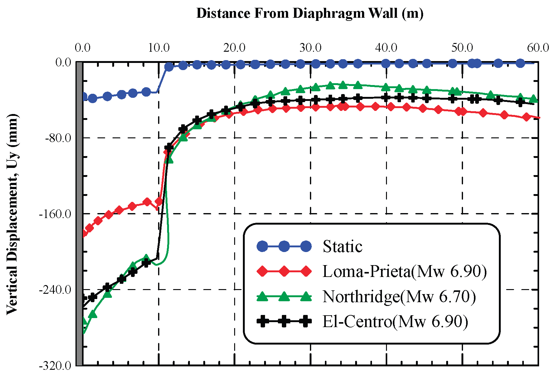
Figure 24.
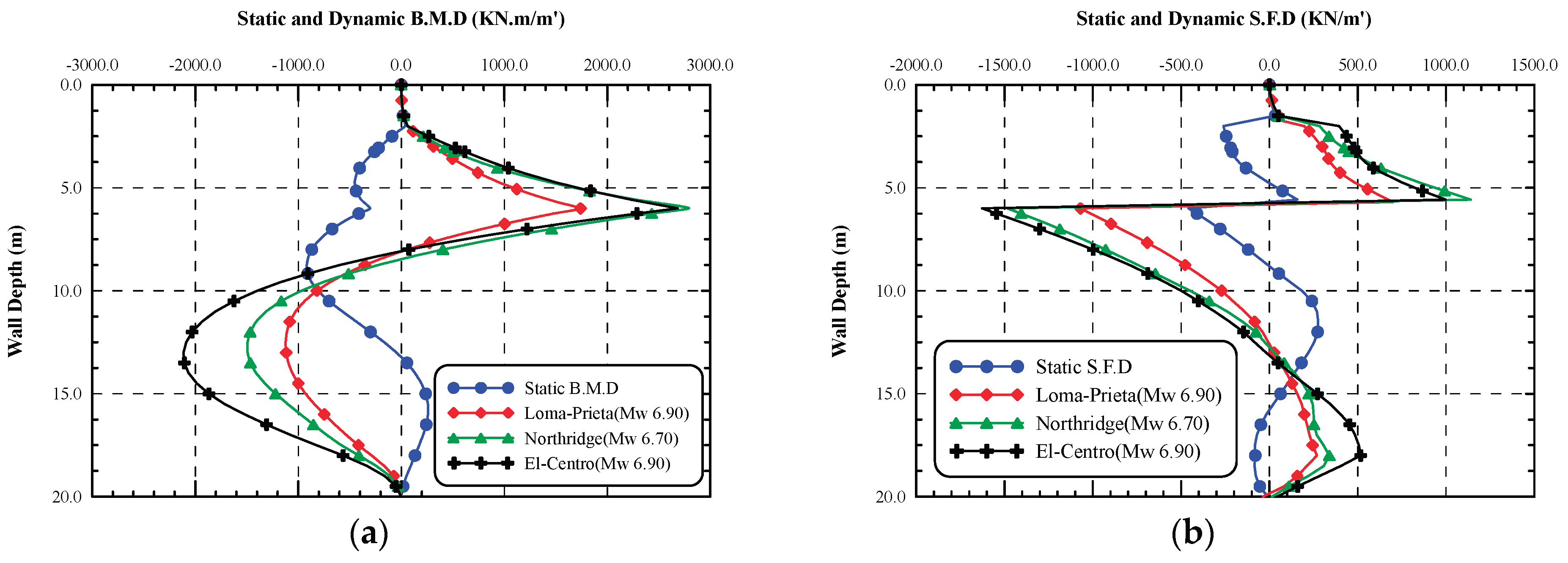
Straining actions along the diaphragm wall in static analysis and for different earthquake records (a and b; bending moment diagram and shear force diagram, respectively).
Figure 24.
Straining actions along the diaphragm wall in static analysis and for different earthquake records (a and b; bending moment diagram and shear force diagram, respectively).
6.2.4. Staining Actions of Diaphragm Wall and Its Supporting Struts
Figure 24.a and 25.b, illustrate the resulting straining actions along the diphragm wall in both static and dynamic analyses. Dynamic bending moment along the diphragm wall shown in Figure 24.a for different earthquakes are of the same pattern, but the amplitude changes due to earthquake intensity and duration. The bending moment under Loma-Prieta earthquake is of the smallest value as compared to the other earthquake records. The bending moment distribution pattern in the dynamic cases looks different than in the static case due to the nature of the dynamic loads that changes its values and direction with time. The maximum static bending moment takes place at 87.5% H from top of diaphragm wall whereas the maxium dynamic bending moment above bottom of excavation level occur at the position of the 2nd strut level and below the bottom of excavation level by nearly 30% D. Below the excavation level, it is noticed that El-Centro has the maximium effect than other earthquakes.
Figure 24.b presents the shearing forces in static and dynamic cases along the diphragm wall. It is notcied that shearing forces of different earthquakes are of the same pattern. The shearing forces under Loma-Prieta earthquake is of the smallest value as compared to the other earthquake records. The maximum shearing forces occurred at the location of the 2nd strut.
Figure 25, investigates the ratio of the maximum dynamic straining actions to the maximum static one. The wall maximum bending moment under Loma-Prieta, Northridge, and El-Centro records are 1.90, 3.04, and 2.93 times the static one, respectively. Moreover, the wall maximum shear force under Loma-Prieta, Northridge, and El-Centro records are 2.34, 3.24, and 3.56 times the static ones, respectively. This increase emphasis the importance of seismic design of such structures.
Figure 26, investigates the resulting axial force in the struts after static and dynamic analyses. As expected, the seismic loads cause large axial forces in the struts. The 2nd strut exabits large axial force than the first one due to the large earth pressure and shearing forces of the wall at this location.
Comparison between the axial forces in the struts under static and dynamic analyses is indicated in Figure 27. The axial force in the 1st level of struts is 1.52, 1.94, and 1.64 times the static ones under Loma-Prieta, Northridge, and El-Centro earthquakes, respectively. Moreover, the axial force in the 2nd level of struts is 4.39, 7.04, and 6.55 times the static ones under Loma-Prieta, Northridge, and El-Centro earthquakes, respectively. Results indicate that Northridge and El-Centro earthquakes have a significant effect on the struts axial force than Loma-Prieta earthquake.
6.2.5. Response of Structure Adjacent to the Shoring System
The storey lateral displacement in static and dynamic cases is indicated in Figure 28. The structure undergoes a lateral displacement in the static case due to excavation process becase of stress relief resulting from removing soil from adjacent to the structure and lateral deformation of the diaphragm wall due to induced lateral earth pressure.
Comaprison between the resulting maximum storey displacement at the base and top of the structure in static and dynamic cases is indicated in Figure 29. The lateral displacement of the base of structure is 3.87, 1.75,and 4.12 times the static one under Loma-Prieta, Northridge, and El-Centro earhquakes, respectively. On the other hand, the lateral displacement of the roof in the dynamic analysis is 4.78, 6.74, and 6.79 times the static one for Loma-prieta, Northridge, and El-Centro earhquakes, respectively.
The large lateral displacement of the structrue in dynamic cases is as a result of large lateral displacement at the top of diaphragm wall in the dynamic analysis. Analysis of the results emphasize that the seismic soil structre interaction between the soil-shoring system and adjacent structures.
7. Conclusions
In this study, 2D numerical non-linear time history analysis using PLAXIS-2D is conducted to investigate the seismic performance of deep braced excavation in sandy soil. The study focuses on the seismic soil-structure-excavation interaction to assess seismic susceptibility of the excavation support system and the adjacent structure. The model is validated against a real case study of deep braced excavation in Kaohsiung City’s central district, adjacent to the O7 Station on the Kaohsiung MRT system’s Orange Line in Taiwan. In parametric study, the following variables are considered: foundation level of the adjacent structure in adjacent to excavation and the response of shoring system and adjacent structure under the effect of Loma-Prieta, Northridge and El-Centro acceleration time histories.
Based on the analysis and discussion of this research the main conclusions of this research are drawn as follows:
- As the building foundation level adjacent to the excavation increases, the permanent ground surface displacement decreases significantly while the displacement at top of diaphragm wall and top of structure increased significantly.
- The dynamic moment increased by an average of 3.32 times the static one while the average increase in shear force during dynamic condition is 2.85 times the static ones.
- The average increase in axial force of the two strut levels because of dynamic forces is 1.38 and 3.17 for the 1st and 2nd struts, respectively, as compared to static ones.
- The dynamic lateral displacement at the top roof is 2.30, 6.18, and 8.37 times than static ones as the foundation level increased from 1.00 m to 5.00 m depth, respectively.
- Loma-Prieta earthquake has a minimal effect on the soil at the ground surface while Northridge has a greater effect of the ground surface. However, El-Centro and Northridge earthquakes have a great effect on the diaphragm wall and the adjacent structure.
- Settlements through dynamic analysis are 5.10, 7.0, and 7.50 times the maximum static ones under Loma-Prieta, Northridge, and El-Centro records, respectively.
- The maximum bending moments under loma-Prieta, Northridge, and El-Centro records are 1.90, 3.04, and 2.93 times the static ones, while the wall maximum shear forces under Loma-Prieta, Northridge, and El-Centro records are 2.34, 3.24, and 3.56 the static ones respectively.
- The axial force in the 1st level of struts is 1.52, 1.94, and 1.64 times the static one under loma-Prieta, Northridge, and El-Centro earthquakes, respectively. However, the axial force in the 2nd level of struts is 4.39, 7.04, and 6.55 times the static one, respectively also.
- The lateral displacements of the base of the structure are 3.87, 1.75, and 4.12 folds the static ones under Loma-Prieta, Northridge, and El-Centro earthquakes respectively. On the other hand, the lateral displacements at the top roof in the dynamic analysis are 4.78, 6.74, and 6.79 times the static ones respectively.
Author Contributions
Tarek N. Salem: Writing—review & editing, Writing—original draft, Conceptualization. Mahmoud S. Almahdy: Writing—review & editing, Data curation, Conceptualization, Writing—original draft. Dušan Katunský: Writing—review & editing, Visualization, Validation, Supervision, Data curation, Conceptualization. Erika Dolnikova: Writing—review & editing, Conceptualization. Ahmed Abu El Ela: Writing—review & editing, Writing—original draft, Methodology, Investigation, Formal analysis, Data curation, Conceptualization.
Funding
This research received no external funding.
Data Availability Statement
Data included in article/supp. material is referenced in the article.
Conflicts of Interest
The authors declare no conflicts of interest.
References
- ACI Committee, 318. (2008). Building code requirements for structural concrete (ACI 318-08) and commentary.
- Arai, Y. , Kusakabe, O., Murata, O., & Konishi, S. (2008). A numerical study on ground displacement and stress during and after the installation of deep circular diaphragm walls and soil excavation. Computers and Geotechnics. 35(5), 791–807. [CrossRef]
- ASCE standard ASCE/SEI 7-16. (2017). Minimum design loads and associated criteria for buildings and other structures. In Minimum Design Loads and Associated Criteria for Buildings and Other Structures. American Society of Civil Engineers. [CrossRef]
- Bahrami, M. Bahrami, M., Khodakarami, M. I., & Haddad, A. (2018). 3D numerical investigation of the effect of wall penetration depth on excavations behavior in sand. Computers and Geotechnics, 98(February), 82–92. [CrossRef]
- Bahrami, M., Khodakarami, M. I., & Haddad, A. (2019). Seismic behavior and design of strutted diaphragm walls in sand. Computers and Geotechnics, 108, 75–87. [CrossRef]
- Benz, T. (2007a). Small-strain stiffness of soils and its numerical consequences (Vol. 5). Univ. Stuttgart, Inst. f. Geotechnik Stuttgart.
- Benz, T. (2007b). Small-Strain Stiffness of Soils and its Numerical Consequences. In University of Stuttgart.
- Boscardin, M. D. , & Cording, E. J. (1992). Building response to excavation-induced settlement. In Journal of Geotechnical Engineering (Vol. 118, Issue 4, pp. 636–637). [CrossRef]
- Bose, S. K., & Som, N. N. (1998). Parametric study of a braced cut by finite element method. Computers and Geotechnics, 22(2), 91–107. [CrossRef]
- Brinkgreve, R. B. J., Bakker, K. J., & Bonnier, P. G. (2006). The relevance of small-strain soil stiffness in numerical simulation of excavation and tunnelling projects. Proceedings of the 6th European Conference on Numerical Methods in Geotechnical Engineering—Numerical Methods in Geotechnical Engineering, 133–139. [CrossRef]
- Brinkgreve, R. B. J., & Vermeer, P. A. (2002). Plaxis finite element code for soil and rock analyses, Version 8. Balkema, Rotterdam. Rotterdam.
- Callisto, L., & Soccodato, F. M. (2010). Seismic design of flexible cantilevered retaining walls. Journal of Geotechnical and Geoenvironmental Engineering, 136(2), 344–354. [CrossRef]
- Callisto, L., Soccodato, F. M., & Conti, R. (2008). Analysis of the Seismic Behaviour of Propped Retaining Structures. Geotechnical Earthquake Engineering and Soil Dynamics IV, 1–10. [CrossRef]
- Castaldo, P., & De Iuliis, M. (2014). Effects of deep excavation on seismic vulnerability of existing reinforced concrete framed structures. Soil Dynamics and Earthquake Engineering, 64, 102–112. [CrossRef]
- Chopra, A. K. (2007). Dynamics of structures. Pearson Education India.
- Chowdhury, S. S., Deb, K., & Sengupta, A. (2013). Estimation of Design Parameters for Braced Excavation: Numerical Study. International Journal of Geomechanics, 13(3), 234–247. [CrossRef]
- Chowdhury, S. S., Deb, K., & Sengupta, A. (2015). Behavior of underground strutted retaining structure under seismic condition. Earthquake and Structures, 8(5), 1147–1170. [CrossRef]
- Chowdhury, S. S., Deb, K., & Sengupta, A. (2016). Effect of Fines on Behavior of Braced Excavation in Sand: Experimental and Numerical Study. International Journal of Geomechanics, 16(1). [CrossRef]
- Chowdhury, S. S., Deb, K., & Sengupta, A. (2017). Estimation of Design Parameters for Braced Excavation in Clays. Geotechnical and Geological Engineering, 35(2), 857–870. [CrossRef]
- El Sawwaf, M. , & Nazir, A. K. (2012). The effect of deep excavation-induced lateral soil movements on the behavior of strip footing supported on reinforced sand. Journal of Advanced Research, 3(4), 337–344. [CrossRef]
- Faheem, H. , Cai, F., & Ugai, K. (2004). Three-dimensional base stability of rectangular excavations in soft soils using FEM. Computers and Geotechnics, 31(2), 67–74. [CrossRef]
- Hardin, B. O. , & Drnevich, V. P. (1972). Shear Modulus and Damping in Soils: Design Equations and Curves. Journal of the Soil Mechanics and Foundations Division, 98(7), 667–692. [CrossRef]
- Hsieh, P.-G., & Ou, C.-Y. (1998a). Shape of ground surface settlement profiles caused by excavation. Canadian Geotechnical Journal, 35(6), 1004–1017.
- Hsieh, P.-G., & Ou, C.-Y. (1998b). Shape of ground surface settlement profiles caused by excavation. Canadian Geotechnical Journal, 35(6), 1004–1017. [CrossRef]
- Hsiung, B. C. B. (2009). A case study on the behaviour of a deep excavation in sand. Computers and Geotechnics, 36(4), 665–675. [CrossRef]
- Hsiung, B. C. B., & Dao, S. D. (2014). Evaluation of constitutive soil models for predicting movements caused by a deep excavation in sands. Electronic Journal of Geotechnical Engineering, 19(Z5), 17325–17344.
- Hughes, T. J. R. (2003). The finite element method: linear static and dynamic finite element analysis. Courier Corporation.
- Huynh, Q. T. , Lai, V. Q., Boonyatee, T., & Keawsawasvong, S. (2021). Behavior of a Deep Excavation and Damages on Adjacent Buildings: a Case Study in Vietnam. Transportation Infrastructure Geotechnology, 8(3), 361–389. [CrossRef]
- Joyner, W. B., & Chen, A. T. F. (1975). Calculation of nonlinear ground response in earthquakes. Bulletin of the Seismological Society of America, 65(5), 1315–1336. http://www.bssaonline.org/content/65/5/1315.abstract.
- Khoiri, M., & Ou, C. Y. (2013). Evaluation of deformation parameter for deep excavation in sand through case histories. Computers and Geotechnics, 47, 57–67. [CrossRef]
- Konai, S., Sengupta, A., & Deb, K. (2018). Behavior of braced excavation in sand under a seismic condition: Experimental and numerical studies. Earthquake Engineering and Engineering Vibration, 17(2), 311–324. [CrossRef]
- Kuhlemeyer, R. L., & Lysmer, J. (1973). Finite element method accuracy for wave propagation problems. Journal of the Soil Mechanics and Foundations Division, 99(5), 421–427. [CrossRef]
- Kung, G. T., Juang, C. H., Hsiao, E. C., & Hashash, Y. M. (2007). Simplified Model for Wall Deflection and Ground-Surface Settlement Caused by Braced Excavation in Clays. Journal of Geotechnical and Geoenvironmental Engineering, 133(6), 731–747. [CrossRef]
- Lam, S. Y., Haigh, S. K., & Bolton, M. D. (2014). Understanding ground deformation mechanisms for multi-propped excavation in soft clay. Soils and Foundations, 54(3), 296–312. [CrossRef]
- Likitlersuang, S., Surarak, C., Wanatowski, D., Oh, E., & Balasubramaniam, A. (2013). Finite element analysis of a deep excavation: A case study from the Bangkok MRT. Soils and Foundations, 53(5), 756–773. [CrossRef]
- Ling, H. I., Leshchinsky, D., Wang, J.-P., Mohri, Y., & Rosen, A. (2009). Seismic Response of Geocell Retaining Walls: Experimental Studies. Journal of Geotechnical and Geoenvironmental Engineering, 135(4), 515–524. [CrossRef]
- Ling, H. I., Liu, H., & Mohri, Y. (2005). Parametric Studies on the Behavior of Reinforced Soil Retaining Walls under Earthquake Loading. Journal of Engineering Mechanics, 131(10), 1056–1065. [CrossRef]
- Ling, H. I., Mohri, Y., Leshchinsky, D., Burke, C., Matsushima, K., & Liu, H. (2005). Large-Scale Shaking Table Tests on Modular-Block Reinforced Soil Retaining Walls. Journal of Geotechnical and Geoenvironmental Engineering, 131(4), 465–476. [CrossRef]
- Liu, G. B., Ng, C. W., & Wang, Z. W. (2005). Observed performance of a deep multistrutted excavation in Shanghai soft clays. Journal of Geotechnical and Geoenvironmental Engineering, 131(8), 1004–1013. [CrossRef]
- Long, M. (2001). Database for retaining wall and ground movements due to deep excavations. Journal of Geotechnical and Geoenvironmental Engineering, 127(3), 203–224. [CrossRef]
- Lysmer, J., Udaka, T., Tsai, C., & Seed, H. B. (1975). FLUSH-A computer program for approximate 3-D analysis of soil-structure interaction problems. California Univ., Richmond (USA). Earthquake Engineering Research Center.
- Madabhushi, S. P. G., & Zeng, X. (2007). Simulating Seismic Response of Cantilever Retaining Walls. Journal of Geotechnical and Geoenvironmental Engineering, 133(5), 539–549. [CrossRef]
- Mikola, R. G. , & Sitar, N. (2013). Seismic Earth Pressures on Retaining Structures in Cohesionless Soils By Roozbeh Geraili Mikola and Nicholas Sitar Report submitted to the California Department of Transportation ( Caltrans ) under Contract No. 65A0367 and NSF-NEES-CR Grant No. CMMI-093. 65, 170. [CrossRef]
- Moormann, C. (2004a). Analysis of wall and ground movements due to deep excavations in soft soil based on a new worldwide database. Soils and Foundations, 44(1), 87–98. [CrossRef]
- Moormann, C. (2004b). Analysis of wall and ground movements due to deep excavations in soft soil based on a new worldwide database. Soils and Foundations, 44(1), 87–98. [CrossRef]
- Obrzud, R. (2010). The hardening soil model: A practical guidebook. zace services.
- Orazalin, Z. Y. , Whittle, A. J., & Olsen, M. B. (2015). Three-Dimensional Analyses of Excavation Support System for the Stata Center Basement on the MIT Campus. Journal of Geotechnical and Geoenvironmental Engineering, 141(7), 1–14. [CrossRef]
- Ou, C.-Y. (2014). Deep excavation: Theory and practice. Crc Press.
- Ou, C.-Y. , Chiou, D.-C., & Wu, T.-S. (1996). Three-dimensional finite element analysis of deep excavations. Journal of Geotechnical Engineering, 122(5), 337–345. [CrossRef]
- Ou, C.-Y., Hsieh, P.-G., & Chiou, D.-C. (1993). Characteristics of ground surface settlement during excavation. Canadian Geotechnical Journal. 30(5), 758–767. [CrossRef]
- Ou, C. Y., & Hsieh, P. G. (2011). A simplified method for predicting ground settlement profiles induced by excavation in soft clay. Computers and Geotechnics, 38(8), 987–997. [CrossRef]
- Ou, C. Y., Hsieh, P. G., & Lin, Y. L. (2013). A parametric study of wall deflections in deep excavations with the installation of cross walls. Computers and Geotechnics, 50, 55–65. [CrossRef]
- PEER. (2022). PEER Ground Motion Database - PEER Center. NGA-West2. https://ngawest2.berkeley.edu/.
- Santos, J., & Correia, A. (2001). Reference threshold shear strain of soil. Its application to obtain an unique strain-dependent shear modulus curve for soil.. XV International Conference on Soil Mechanics and Geotechnical Engineering, 267–270. https://www.cabidigitallibrary.org/doi/full/10.5555/20023124705.
- Tufenkjian, M. R., & Vucetic, M. (2000). Dynamic Failure Mechanism of Soil-Nailed Excavation Models in Centrifuge. Journal of Geotechnical and Geoenvironmental Engineering, 126(3), 227–235. [CrossRef]
- Wang, J. H., Xu, ; Z H, & Wang, W. D. (n.d.). Wall and Ground Movements due to Deep Excavations in Shanghai Soft Soils. [CrossRef]
- Yeganeh, N. , Bolouri Bazaz, J., & Akhtarpour, A. (2015). Seismic analysis of the soil-structure interaction for a high rise building adjacent to deep excavation. Soil Dynamics and Earthquake Engineering, 79, 149–170. [CrossRef]
- Yoo, C. , & Lee, D. (2008). Deep excavation-induced ground surface movement characteristics—A numerical investigation. Computers and Geotechnics, 35(2), 231–252. [CrossRef]
- Zdravkovic, L., Potts, D. M., & St John, H. D. (2011). Modelling of a 3D excavation in finite element analysis. Stiff Sedimentary Clays: Genesis and Engineering Behaviour - Geotechnique Symposium in Print 2007, 7, 319–335. [CrossRef]
- Zienkiewicz, O. C., Bicanic, N., & Shen, F. Q. (1989). Earthquake Input Definition and the Trasmitting Boundary Conditions. In Advances in Computational Nonlinear Mechanics (pp. 109–138). Springer Vienna. [CrossRef]
- Zienkiewicz, O. C., & R.L. Taylor. (1991). The finite element method. Vol. 2 : Solid and fluid mechanics, dynamics and non-linearity. In The finite element method. Vol. 2 : (4th ed.). McGraw-Hil.
Figure 1.
Location of the case study.
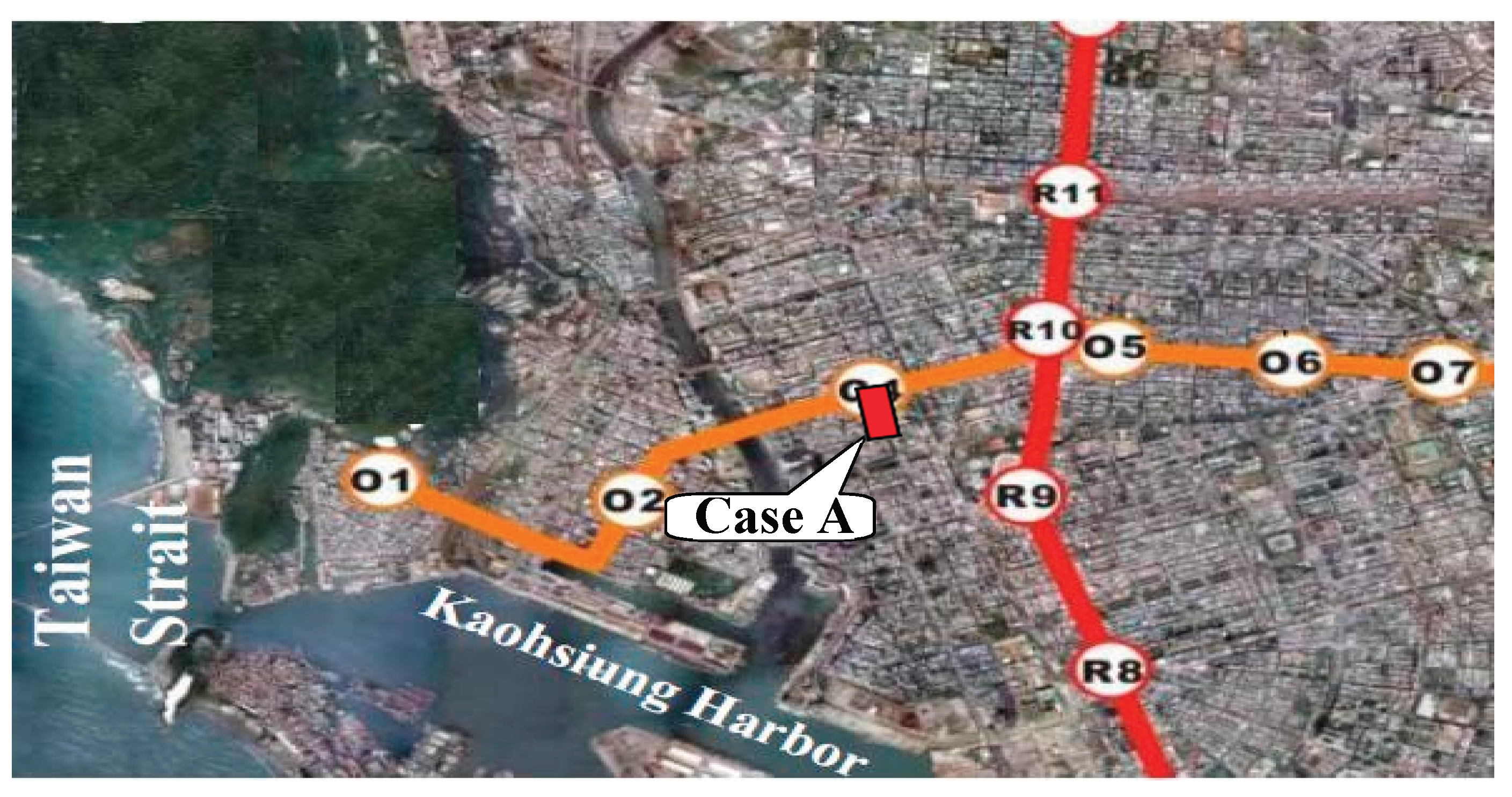
Figure 2.
Ground layers and properties and the excavation cross-section, as reported in (Hsiung & Dao, 2014).
Figure 2.
Ground layers and properties and the excavation cross-section, as reported in (Hsiung & Dao, 2014).
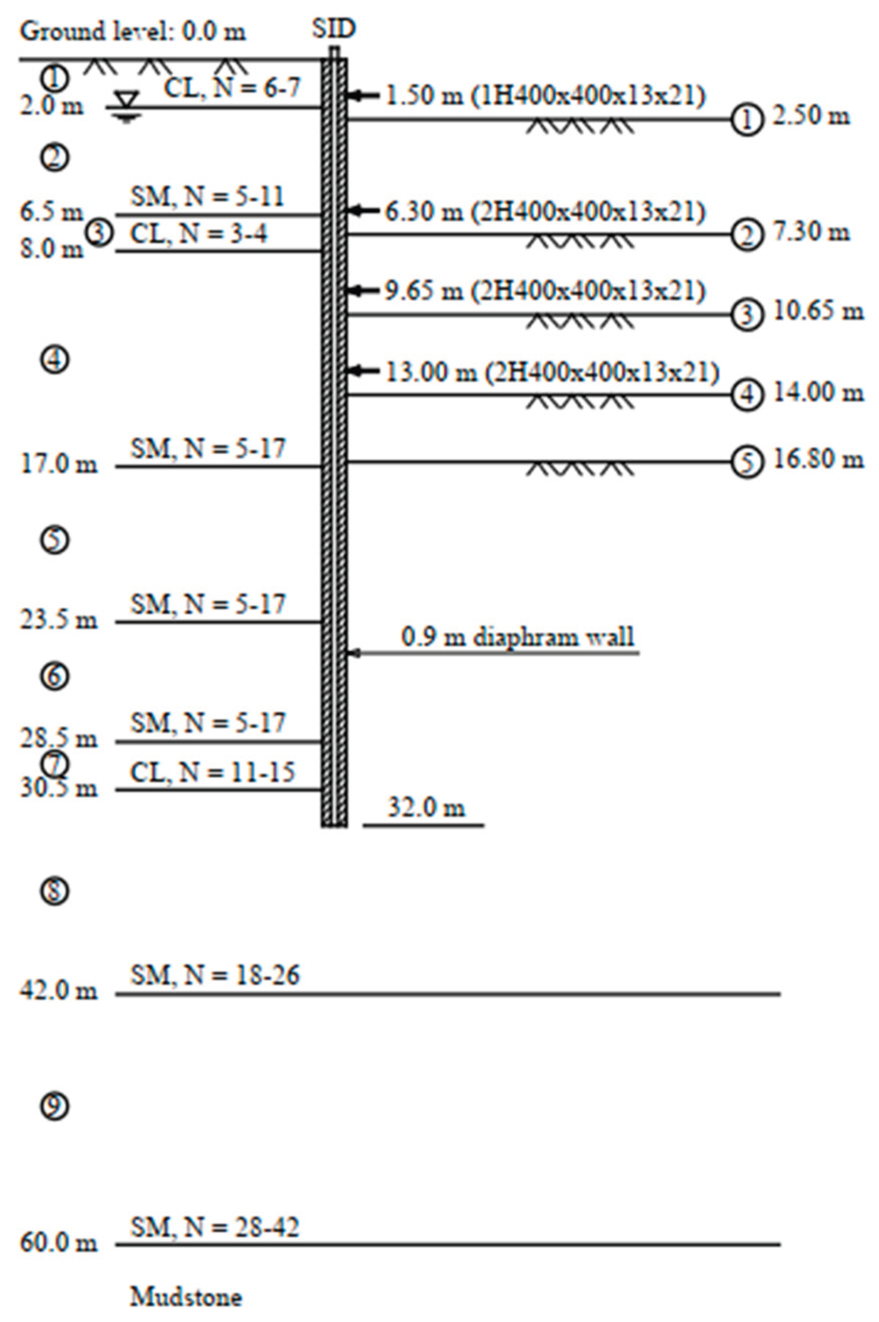
Figure 3.
Measured lateral displacement of the wall and the settlements at the excavation site.
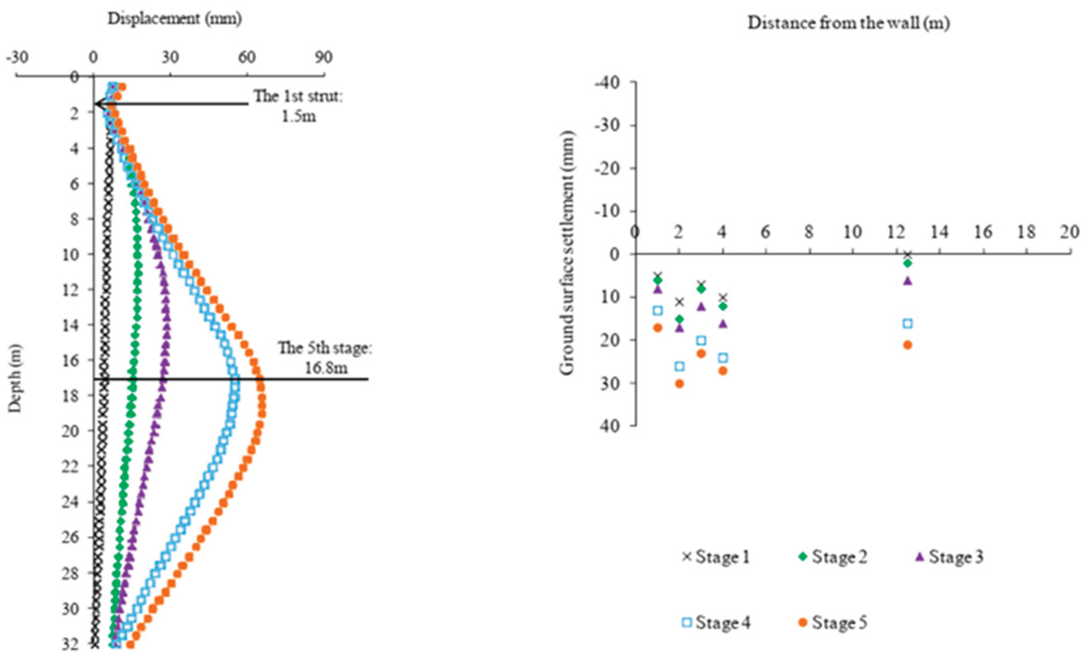
Figure 4.
Verification model geometry, soil stratigraphy and mesh discretization with boundary conditions.
Figure 4.
Verification model geometry, soil stratigraphy and mesh discretization with boundary conditions.
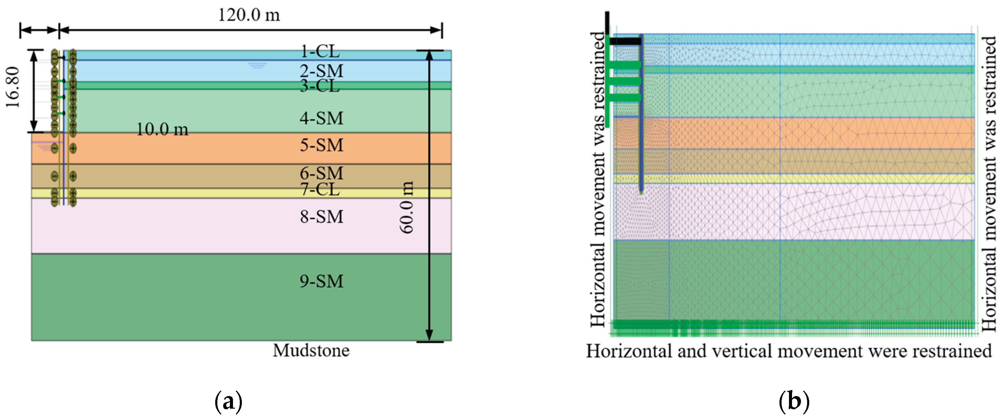
Figure 5.
Comparison between the measured and the predicted lateral wall displacement at the final stage of excavation.
Figure 5.
Comparison between the measured and the predicted lateral wall displacement at the final stage of excavation.
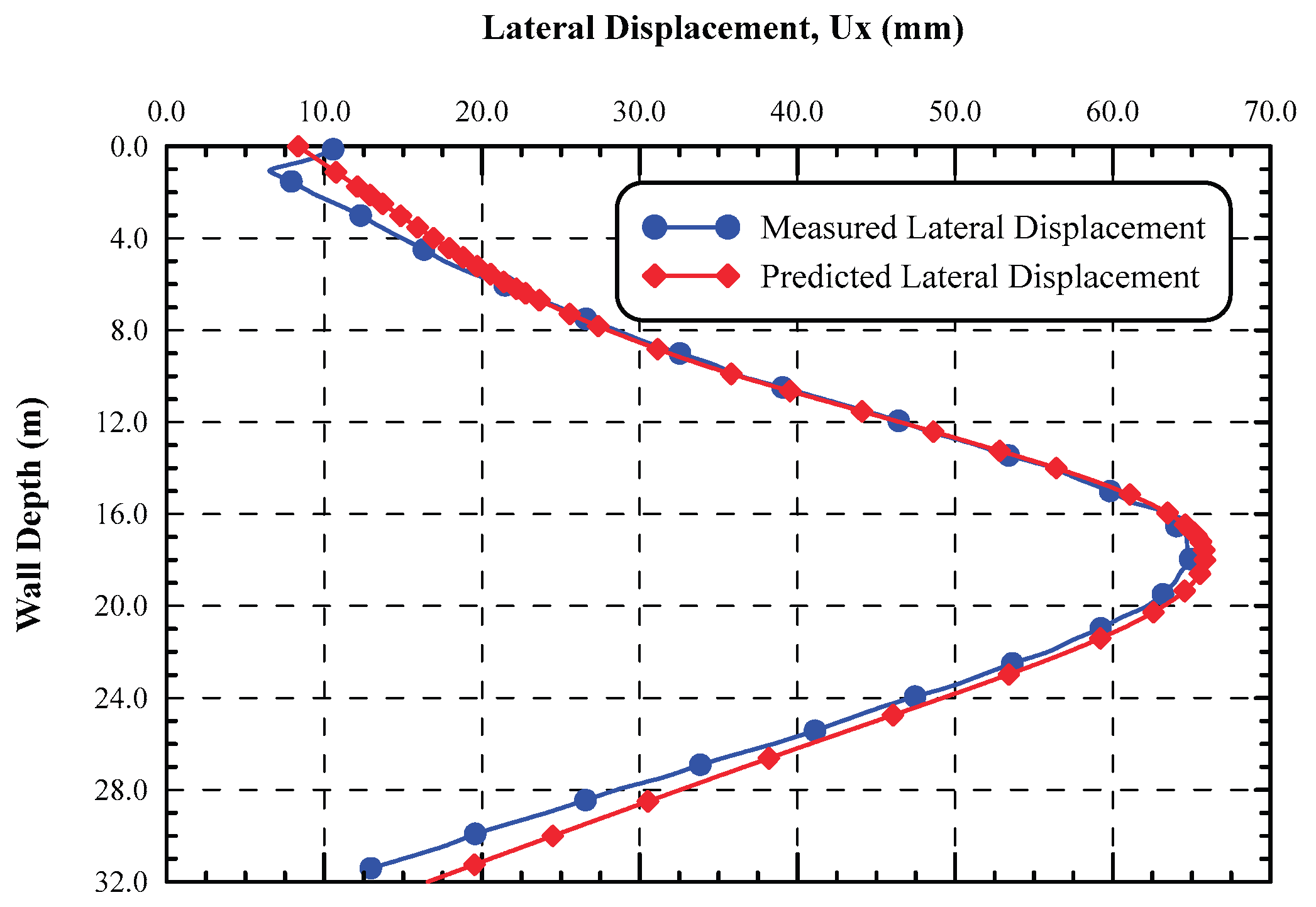
Figure 6.
Comparison of the measured and the predicted ground surface settlement at all excavation stages.
Figure 6.
Comparison of the measured and the predicted ground surface settlement at all excavation stages.
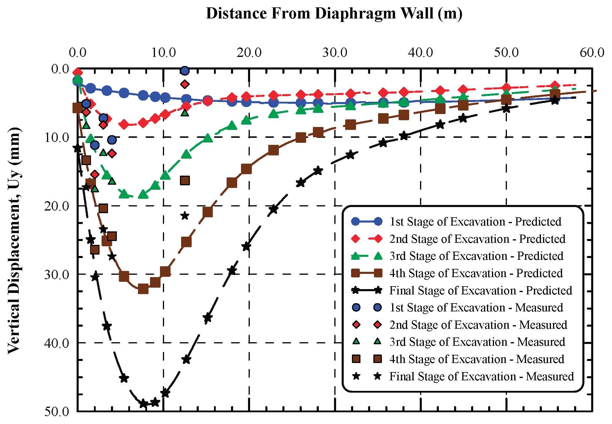
Figure 7.
Model geometry, mesh discretization and boundary condition of the case study in parametric study.
Figure 7.
Model geometry, mesh discretization and boundary condition of the case study in parametric study.
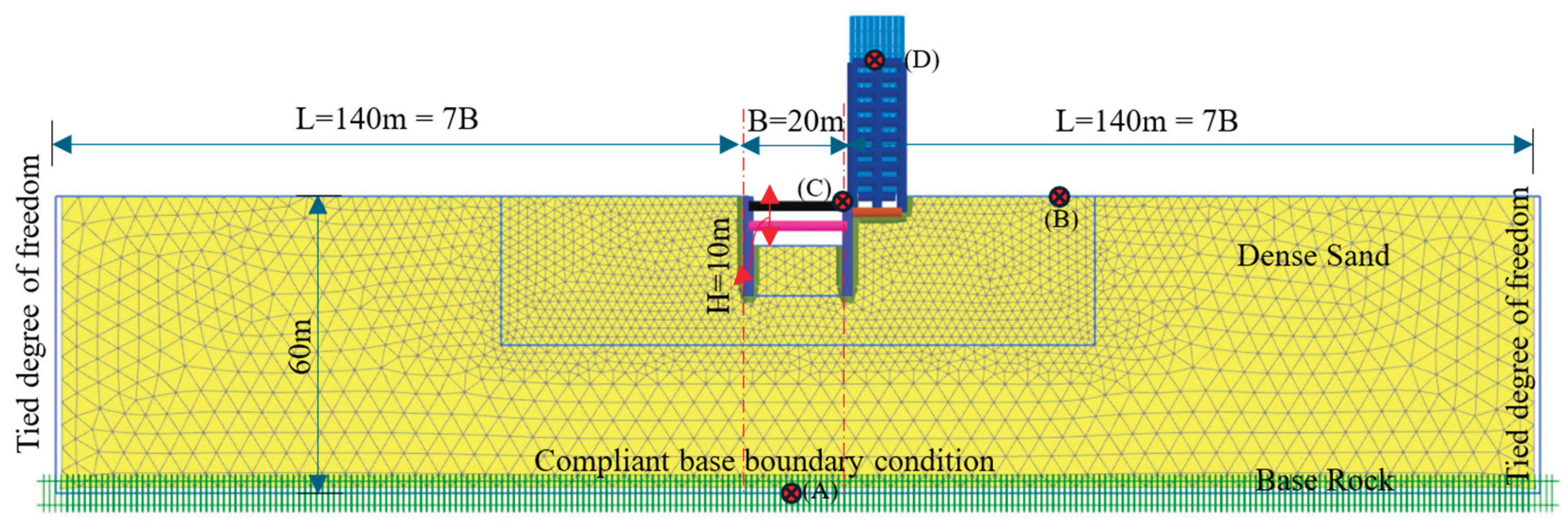
Figure 10.
Displacement-time history for different structure foundation levels (a,b and c; free field ground surface, top of diaphragm wall, and top roof of structure, respectively).
Figure 10.
Displacement-time history for different structure foundation levels (a,b and c; free field ground surface, top of diaphragm wall, and top roof of structure, respectively).
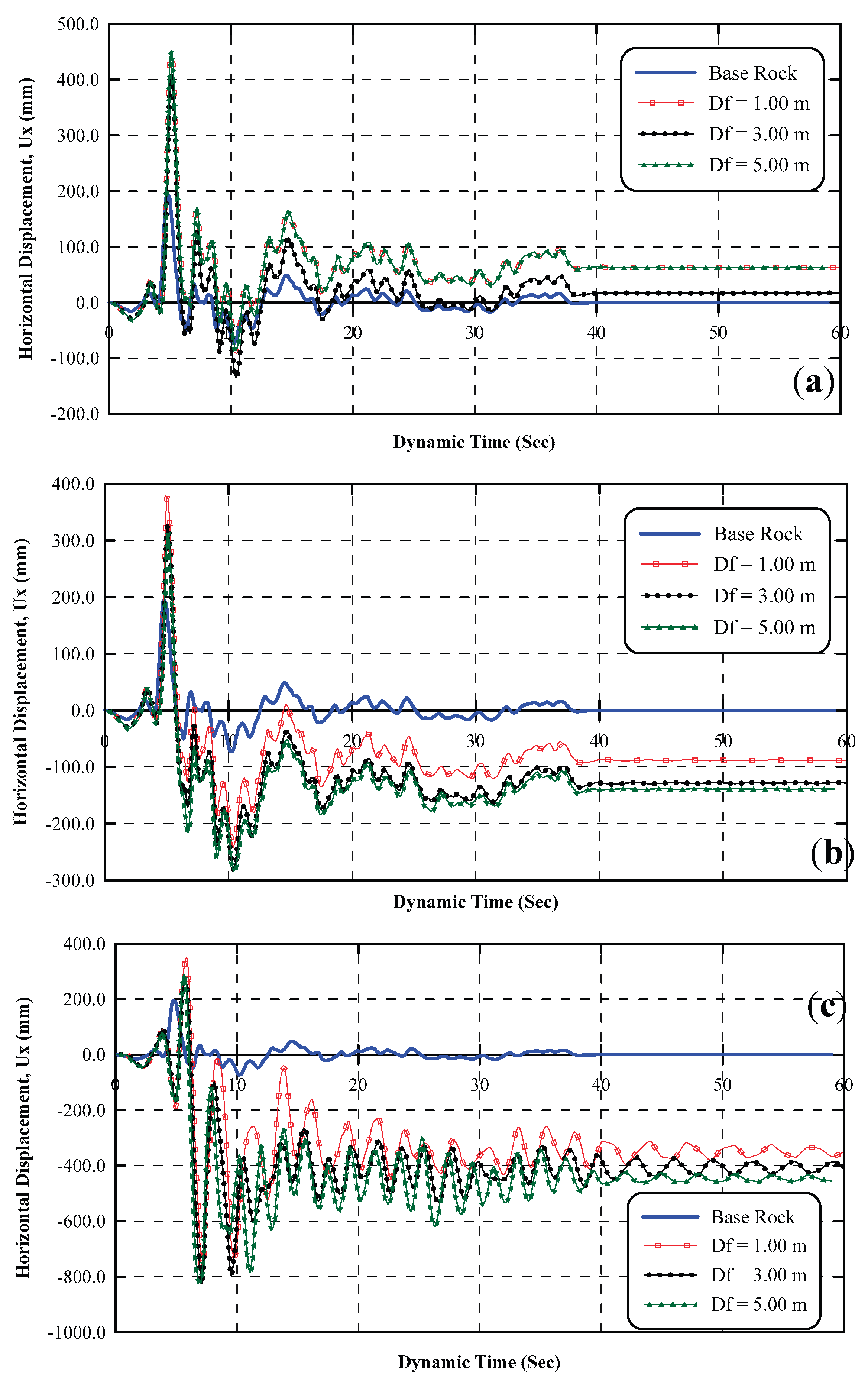
Figure 11.
Settlement trough for different foundation levels of the structure (a, b; static and dynamic analysis, respectively).
Figure 11.
Settlement trough for different foundation levels of the structure (a, b; static and dynamic analysis, respectively).
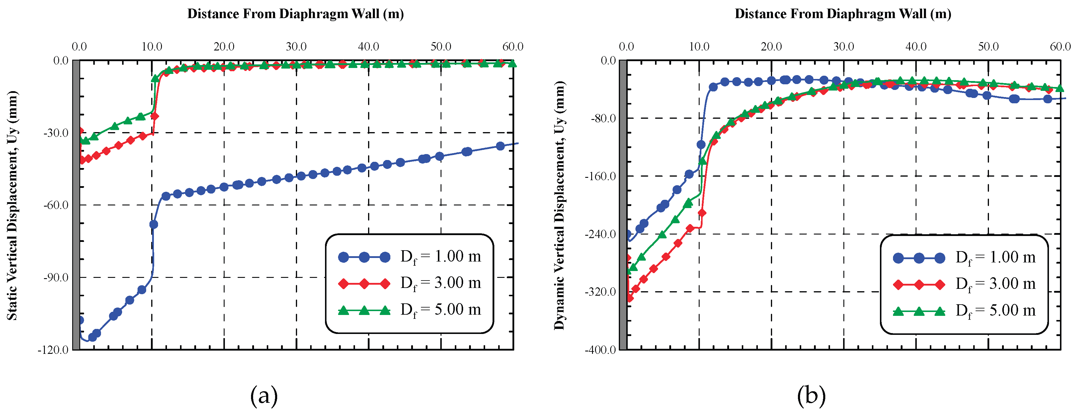
Figure 12.
Lateral displacement of the diaphragm wall under different Foundation Levels of the adjacent structure(a and b; static lateral displacement and dynamic one, respectively).
Figure 12.
Lateral displacement of the diaphragm wall under different Foundation Levels of the adjacent structure(a and b; static lateral displacement and dynamic one, respectively).
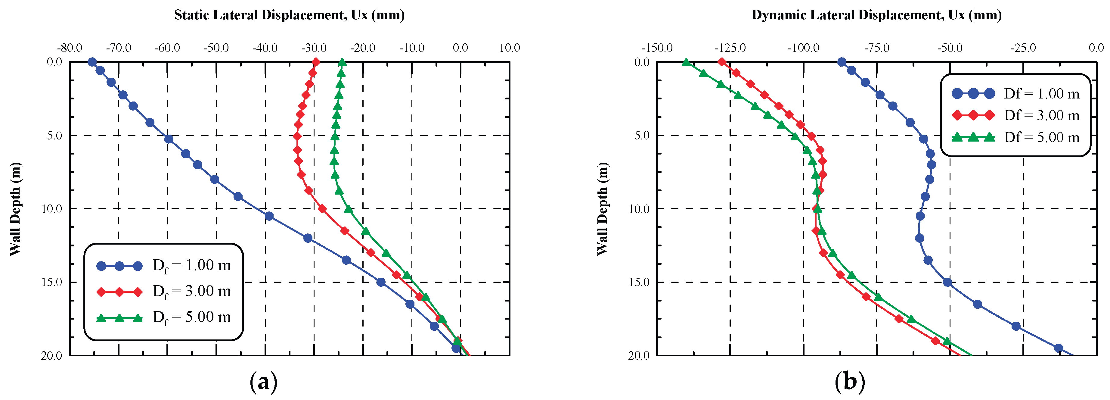
Figure 13.
Comparison between the lateral displacement at the top of the diaphragm wall in static and dynamic cases for different Foundation Level of the adjacent structure.
Figure 13.
Comparison between the lateral displacement at the top of the diaphragm wall in static and dynamic cases for different Foundation Level of the adjacent structure.
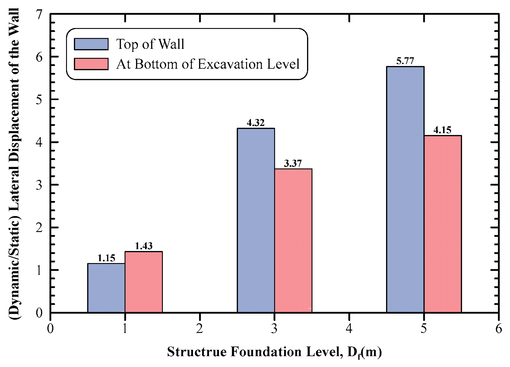
Figure 14.
Diaphragm wall straining actions in static and dynamic cases for different Foundation Level of structure (a, b, c, and d; static bending moment, dynamic bending moment, static shear force, and dynamic shear force, respectively).
Figure 14.
Diaphragm wall straining actions in static and dynamic cases for different Foundation Level of structure (a, b, c, and d; static bending moment, dynamic bending moment, static shear force, and dynamic shear force, respectively).
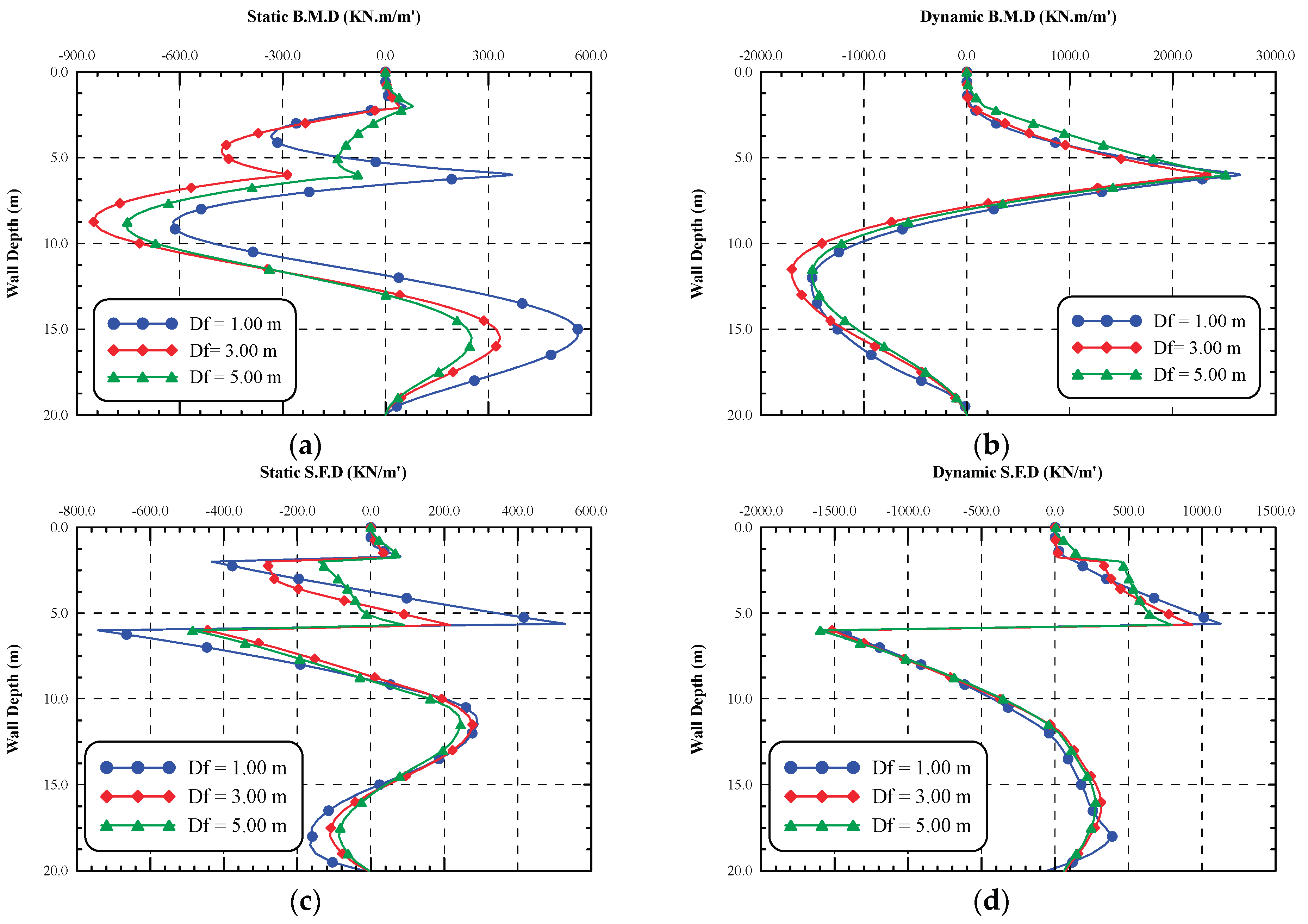
Figure 15.
Comparison between dynamic and static maximum straining actions along the diaphragm wall for different foundation levels of structure.
Figure 15.
Comparison between dynamic and static maximum straining actions along the diaphragm wall for different foundation levels of structure.
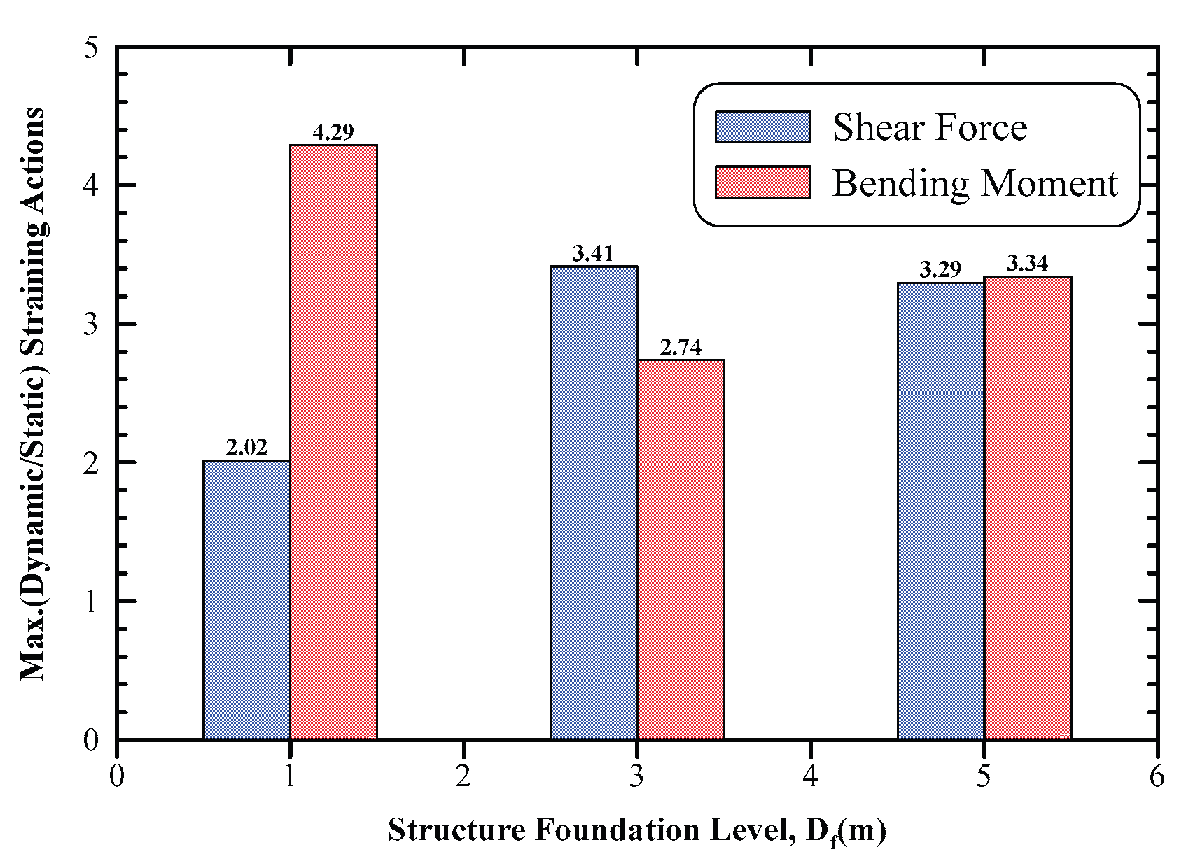
Figure 16.
Axial force in the struts in both static and dynamic cases for different foundation levels of the structure.
Figure 16.
Axial force in the struts in both static and dynamic cases for different foundation levels of the structure.
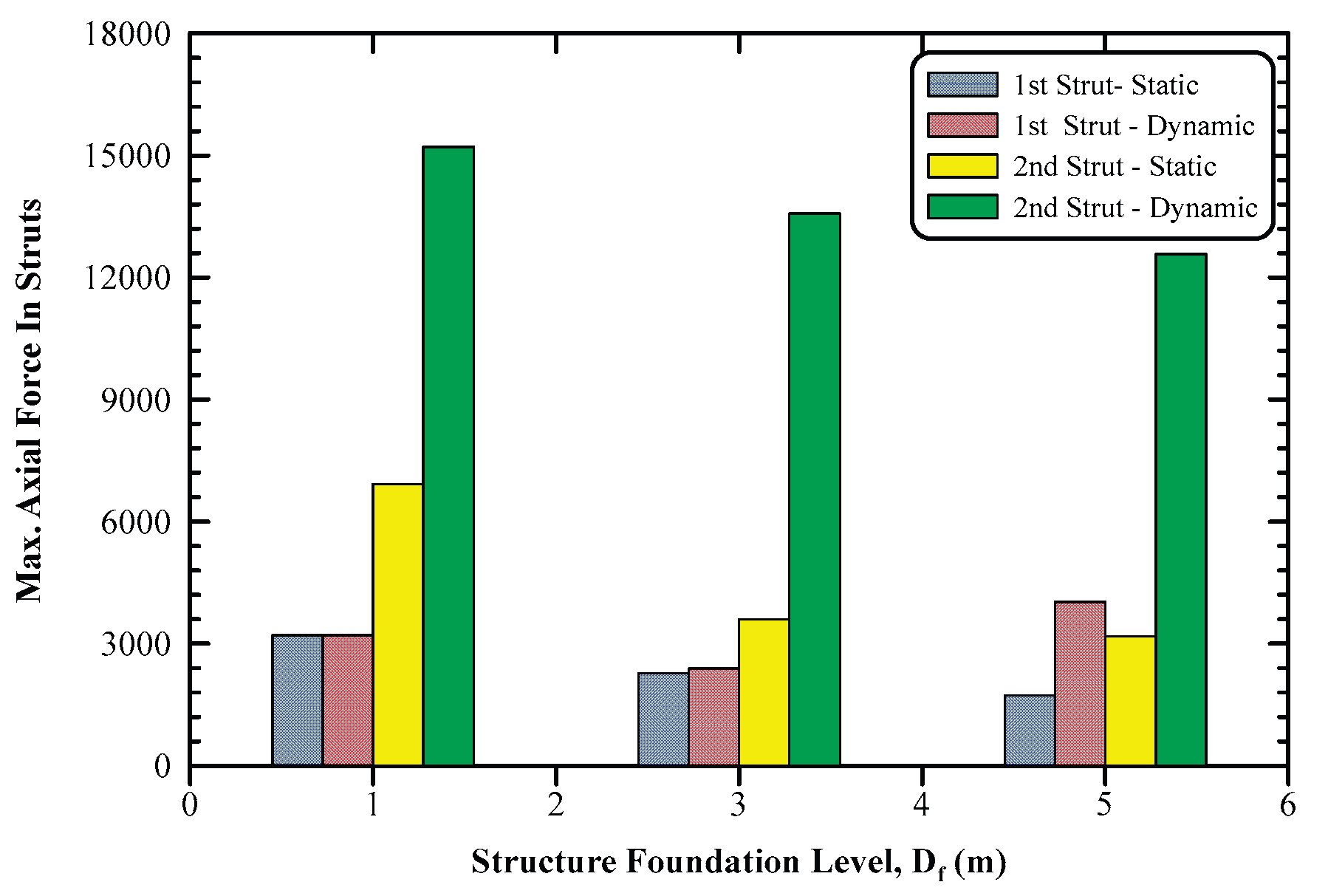
Figure 17.
Comparison between the maximum axial forces in struts in dynamic and static cases for different foundation levels of structure.
Figure 17.
Comparison between the maximum axial forces in struts in dynamic and static cases for different foundation levels of structure.
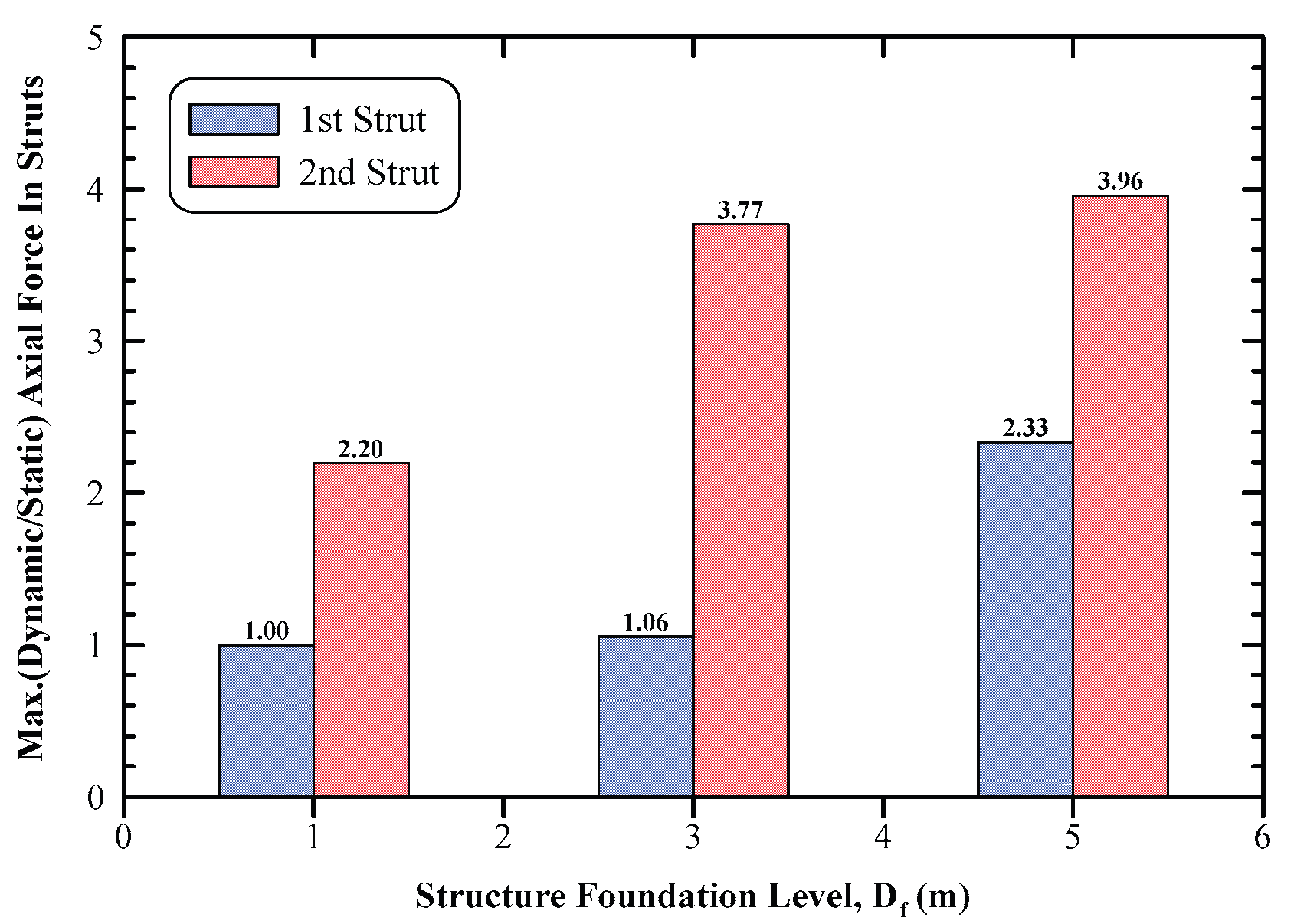
Figure 18.
Structure storey displacement in static and dynamic cases for different foundation levels (a and b; static case and dynamic case, respectively).
Figure 18.
Structure storey displacement in static and dynamic cases for different foundation levels (a and b; static case and dynamic case, respectively).
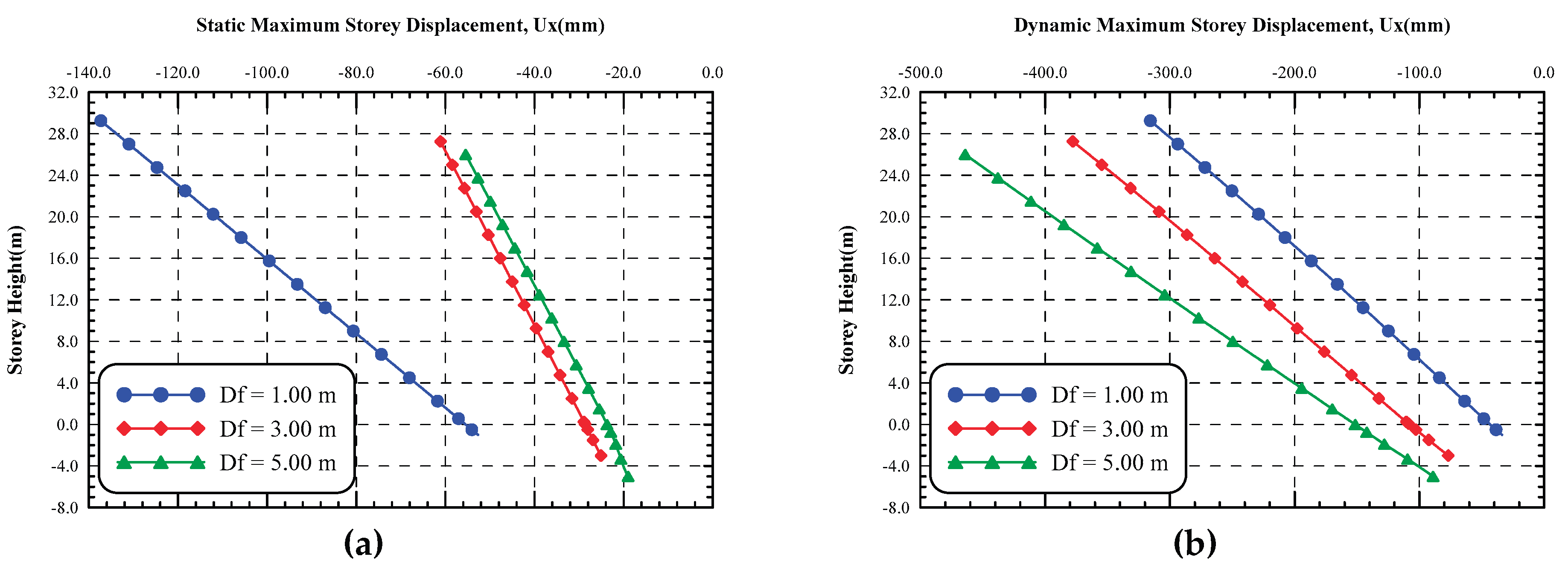
Figure 19.
Comparison between dynamic and static maximum storey displacement at the top roof and at the base of structure for different structure Foundation Levels.
Figure 19.
Comparison between dynamic and static maximum storey displacement at the top roof and at the base of structure for different structure Foundation Levels.
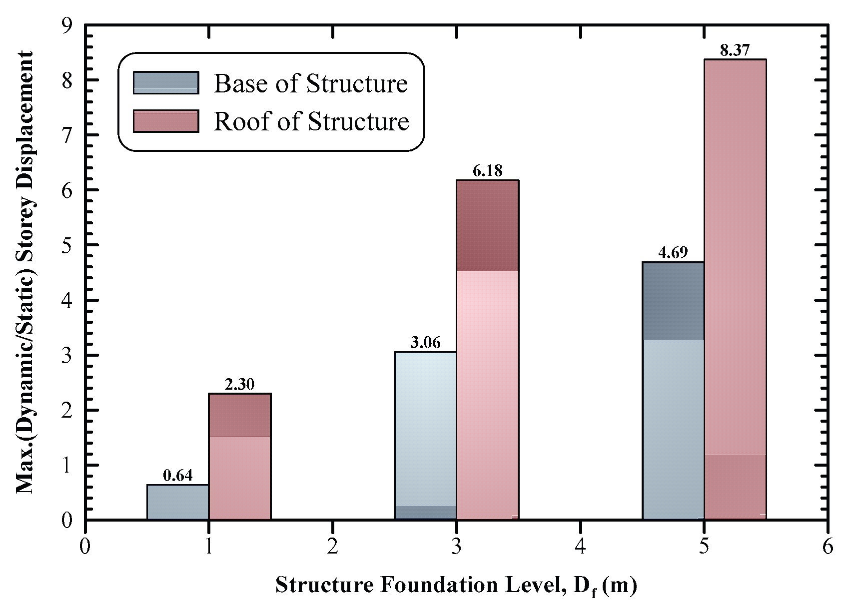
Figure 20.
Displacement time history of base ground motion, the ground surface free field motion, the top of diaphragm wall, and the top of the structure adjacent to the excavation (a, b, and c; using Loma-Prieta, Northridge, and El-Centro earthquakes, respectively).
Figure 20.
Displacement time history of base ground motion, the ground surface free field motion, the top of diaphragm wall, and the top of the structure adjacent to the excavation (a, b, and c; using Loma-Prieta, Northridge, and El-Centro earthquakes, respectively).
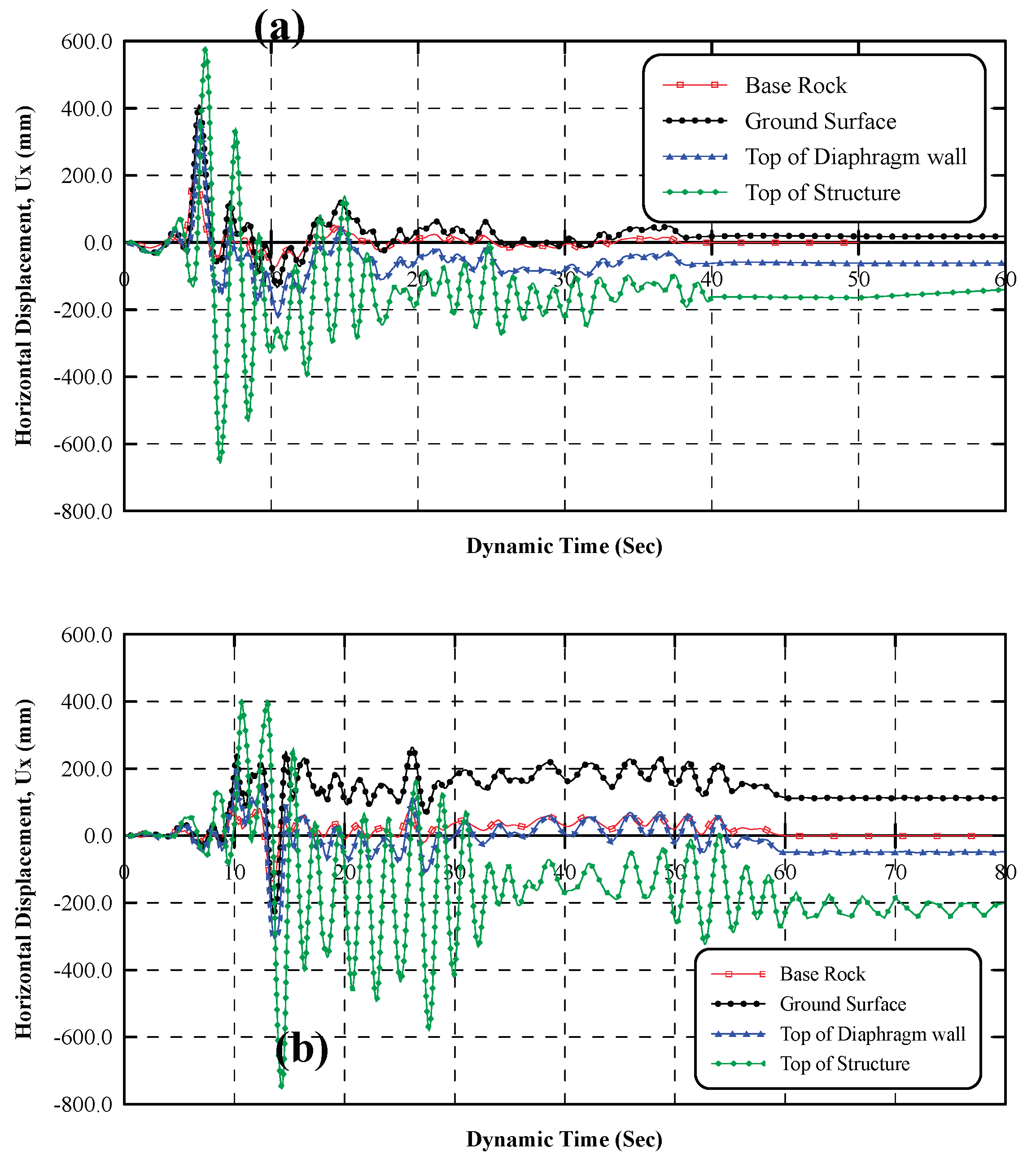
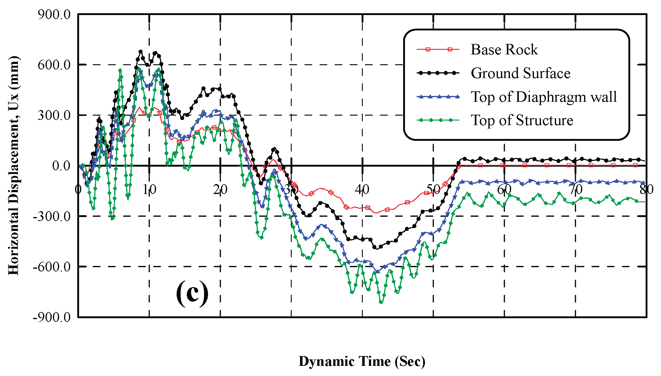
Figure 21.
The lateral displacement of the diaphragm wall under static and under Loma-Prieta, Northridge, and El-Centro Earthquake Records.
Figure 21.
The lateral displacement of the diaphragm wall under static and under Loma-Prieta, Northridge, and El-Centro Earthquake Records.

Figure 22.
(Dynamic/static) lateral displacement ratio for different earthquake records.
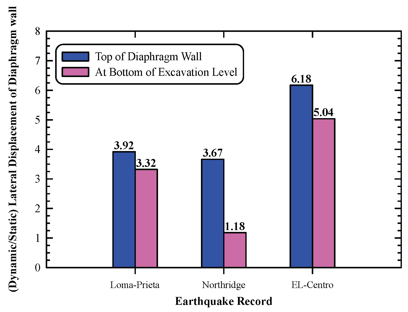
Figure 25.
comparison between the increase in dynamic straining actions than the static ones under different earthquake records.
Figure 25.
comparison between the increase in dynamic straining actions than the static ones under different earthquake records.
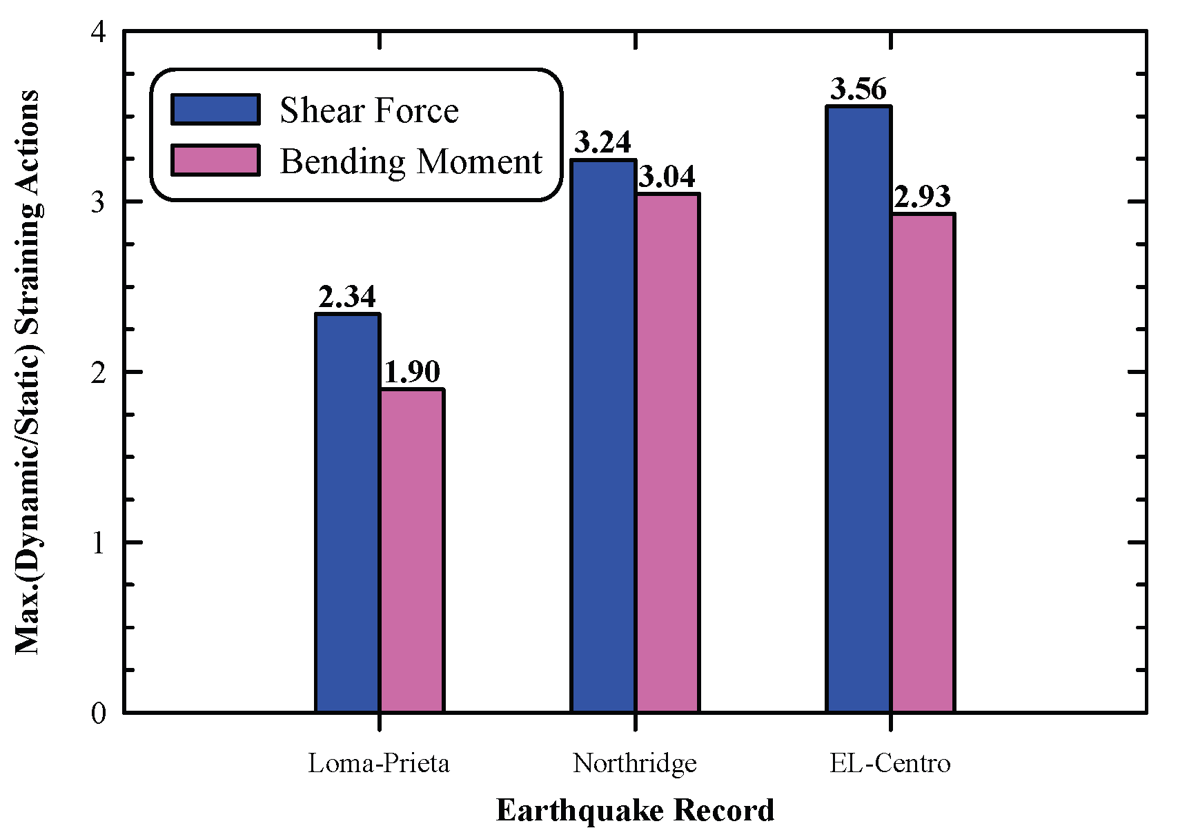
Figure 26.
The axial force in the struts in static and under different earthquake ground motions.
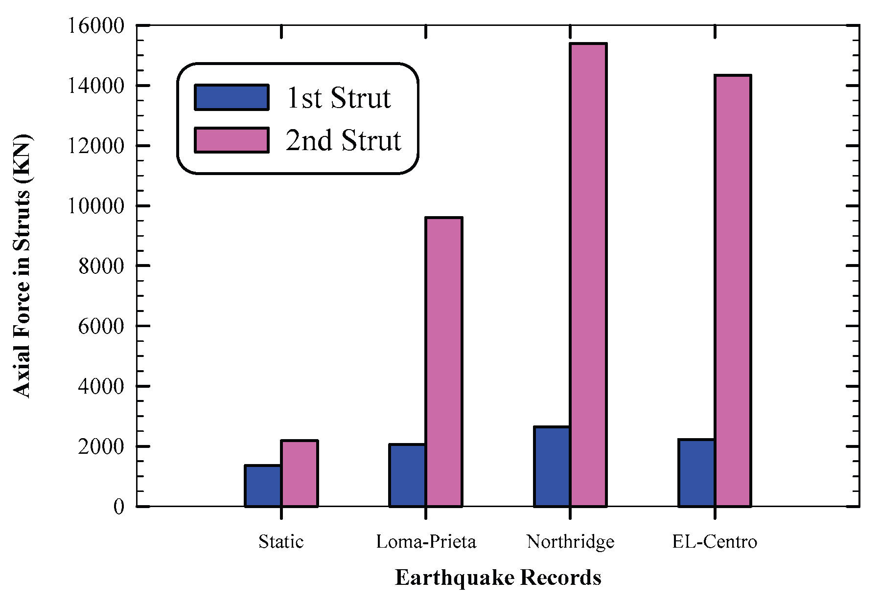
Figure 27.
Comparison between the axial forces in the struts under different earthquake ground motions.
Figure 27.
Comparison between the axial forces in the struts under different earthquake ground motions.
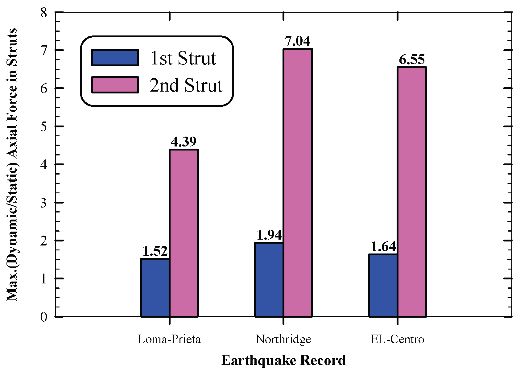
Figure 28.
The storey lateral displacement distribution in static and in dynamic case.
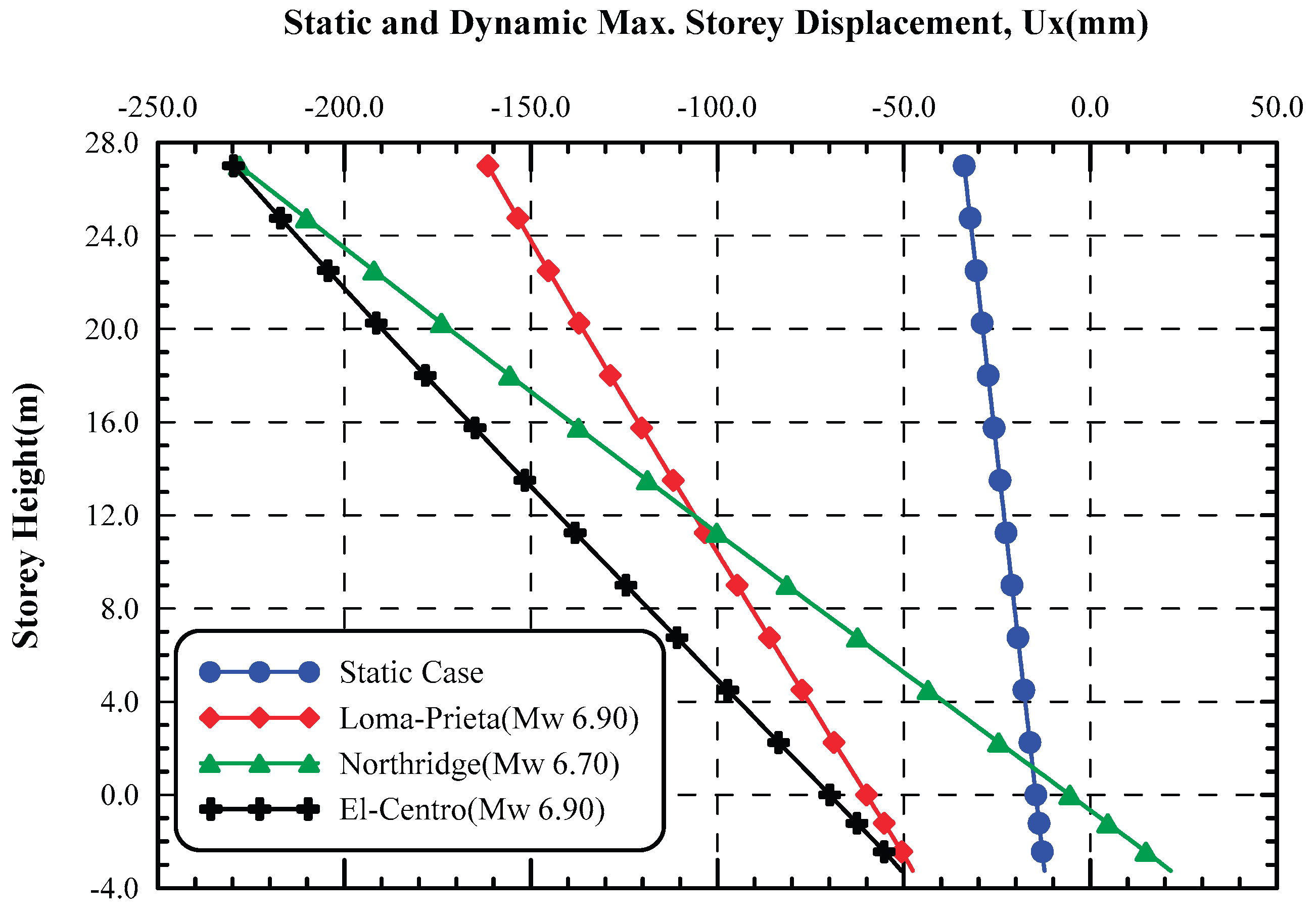
Figure 29.
Comparison between the maximum storey displacement at the base and top roof of structure in static and dynamic cases.
Figure 29.
Comparison between the maximum storey displacement at the base and top roof of structure in static and dynamic cases.
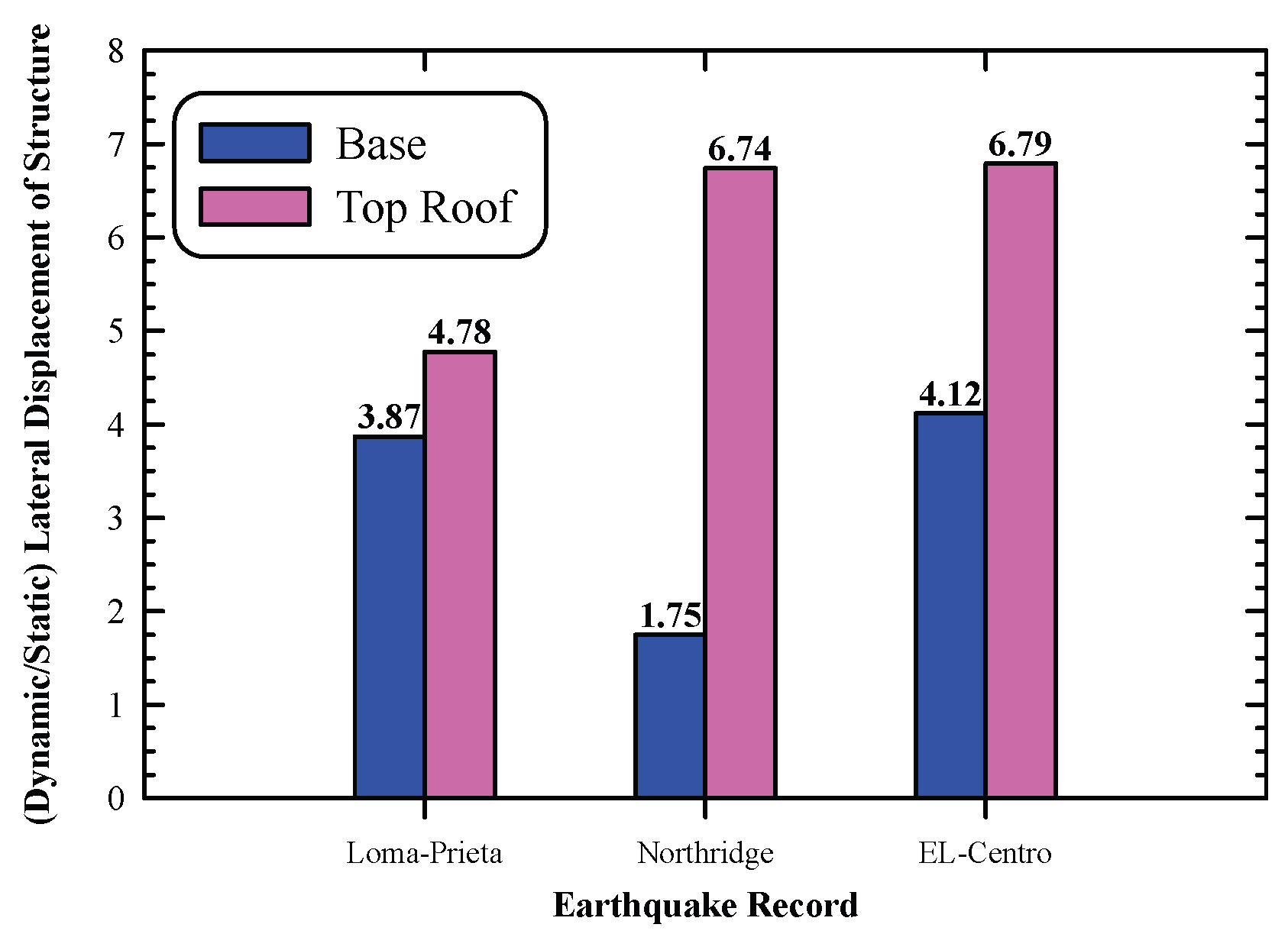
Table 3.
Soil properties used in the parametric study of the dense sand layer using HS-small model.
| Depth of layer (m) | 60 |
| Soil Type | Dense Sand |
| SPT (N-Value) | 37 |
| Soil Model | Hardening soil model with small strain (HS small) |
| unsat (KN/m3) | 19 |
| sat (KN/m3) | 21 |
| Rayleigh damping (α) | 0.1634 |
| Rayleigh damping (β) | 1.662 × 10⁻³ |
| Damping Ratio | 2 % |
| Internal friction angle | 36 |
| Cohesion, | 1 |
| Dilatancy angle Ψ | 6 |
| Reference secant stiffness from drained triaxial test | 50,000 |
| Reference tangent stiffness for oedometer primary loading | 50,000 |
| Reference unloading/reloading stiffness | 150,000 |
| Unloading/reloading Poisson’s Ratio ν‘ur |
0.20 |
| Power for stress-level dependency of stiffness, m | 0.50 |
| Failure ratio, Rf | 0.90 |
| At rest earth pressure coefficient | 0.4122 |
| Reference small strain shear modulus, G0 ref (Kpa) | 180,000 |
| Shear strain magnitude at 0.722G0, γ0.7 | 1 × 10⁻⁴ |
| Analysis Type | Drained |
| Rinter | 0.67 |
Table 4.
Summary of the studied parameters.
| Studied Parameter | The parameter variables | chosen parameters |
| Foundation Level of structure adjacent to shoring system | Df = 1.0 m | H = 10 m B = 20 m, Tw = 80 cm D = H = 10 m Loma-Prieta EQ |
| Df = 3.0 m | ||
| Df = 5.0 m | ||
| Earthquake Records | Loma-Prieta (1989), Mw = 6.90 | H = D = 10 m Tw = 80 cm B = 20m |
| Northridge (1994), Mw = 6.70 | ||
| El-Centro (1940), Mw=6.90 | ||
| H = The final excavation depth B = Width of excavation Tw = Diaphragm wall thickness D = Diaphragm wall embedment depth Df = Foundation level of the adjacent structure | ||
Table 5.
Properties of input earthquake ground motions:.
| Earthquake Record | Moment magnitude (Mw) |
PGA (g) |
Duration (sec) |
Predominant period, Tp (sec) |
Arias intensity, Ia (m/s) | Significant duration, Ds 5-95 (sec) |
| Loma-Prieta (1989) | 6.90 | 0.37 | 39.90 | 0.22 | 1.35 | 11.37 |
| Northridge (1994) | 6.70 | 0.88 | 60.00 | 0.22 | 2.72 | 8.75 |
| El-Centro (1940) | 6.90 | 0.34 | 53.76 | 0.56 | 1.76 | 24.46 |
Disclaimer/Publisher’s Note: The statements, opinions and data contained in all publications are solely those of the individual author(s) and contributor(s) and not of MDPI and/or the editor(s). MDPI and/or the editor(s) disclaim responsibility for any injury to people or property resulting from any ideas, methods, instructions or products referred to in the content. |
© 2025 by the authors. Licensee MDPI, Basel, Switzerland. This article is an open access article distributed under the terms and conditions of the Creative Commons Attribution (CC BY) license (http://creativecommons.org/licenses/by/4.0/).
Copyright: This open access article is published under a Creative Commons CC BY 4.0 license, which permit the free download, distribution, and reuse, provided that the author and preprint are cited in any reuse.


