
Submitted:
28 January 2026
Posted:
29 January 2026
You are already at the latest version
Abstract
Performance‑based evaluation of reinforced soil retaining structures often relies on numerical analyses that require substantial time and expert judgment due to the complex interactions among soils, reinforcements, facings, and seismic loading. This study presents an efficient approach for developing seismic resisting capacity curves for reinforced slopes using a computer program based on the Force Equilibrium Finite Displacement Method (FFDM). The resulting curves resemble the monotonic pushover curves widely used in structural engineering, indicating that the framework is aligned with established performance‑based methodologies. The method is demonstrated by revisiting the Tanada Wall, a geosynthetic reinforced soil retaining wall with a full height rigid facing that experienced strong shaking during the 1995 Hyogoken Nambu earthquake (ML = 7.2). Using parameters available in published databases, the FFDM generates realistic seismic resistance curves and directly computes seismic displacements. Three advantages distinguish the FFDM from LEM based Newmark approaches: explicit incorporation of peak soil strength and post peak degradation along the slip surface; direct use of peak ground acceleration (HPGA/g) as input, avoiding uncertainties in selecting representative seismographs; and capability for back analysis, enabling soil parameters calibrated from small observed displacements to be used for predicting performance under stronger shaking. A conceptual back analysis procedure is introduced to illustrate this potential.
Keywords:
finite displacement method (FFDM)
; seismic displacement
; geosynthetic-reinforced soil structures
; seismic resistance curves
; retaining wall
; back-analysis
1. Introduction
In conventional engineering practice, the seismic stability of slopes is commonly evaluated using the safety factor (Fs) derived from prescribed seismic coefficients (kh) through limit equilibrium methods (LEM). To estimate seismic-induced slope displacements, Newmark’s hybrid approach—described in [1]—combines LEM with sliding block dynamics and remains widely adopted. A key requirement for applying Newmark’s method is the determination of a calibrated critical seismic coefficient (khc), obtained from the Fs–kh relationship at the condition Fs = 1.0. Identifying this khc typically involves iterative trial-and-error adjustments to determine an “operational” internal friction angle (φ) that produces a satisfactory Fs–kh curve. Despite the use of double integration of ground acceleration based on dynamic principles, Newmark’s approach remains fundamentally pseudo-static because the essential parameter khc is determined through a pseudo-static framework. Over the past decades, numerous studies have sought to enhance the performance and applicability of Newmark’s method. These efforts can be broadly categorized as follows:
(1) improving the accuracy of the yield (critical) seismic coefficient by adopting analytical formulations beyond those used in conventional LEM or by introducing alternative failure mechanisms [2,3,4,5,6,7]
(2) improving the post-yield response of the sliding mass using dynamic analyses with single- or multi-degree-of-freedom systems [8,9,10,11,12,13]
(3) incorporating deformability of the sliding mass through springs, dashpots, or multiple sliding layers [14,15,16,17,18]
(4) extending the method to engineered slopes with different failure mechanisms or reinforcement types [19,20,21,22,23]
(5) introducing multiple sliding blocks to capture interaction effects within the failure mass [21,24,25]
(6) accounting for nonlinear soil behavior, strength degradation, and evolving slip-surface geometry [26,27,28,29,30]
(7) considering changes in failure mechanisms under different shaking intensities [31] .
Although these studies have substantially advanced the theoretical framework of Newmark-type analyses, several issues limit their practical applicability in geotechnical design. First, Newmark-based methods are valid only when seismic accelerations exceed the critical (yield) acceleration; displacement is assumed zero in the pre-yield state, contradicting observed behavior [17]. As a result, a unified description of soil–structure response across static, pre-yield, and post-yield states is not feasible. Second, improving the accuracy of yield acceleration or incorporating deformability typically requires additional soil parameters—such as spring stiffness or damping constants—and assumptions regarding lumped masses. These parameters often require specialized laboratory testing, and the mass discretization introduces further empiricism. Third, many modified approaches rely on simplified sliding blocks on single-inclination planes or on lumped masses without internal interaction, which does not adequately represent real failures involving curved slip surfaces and lateral thrusts among soil slices. To overcome the inherent limitations of pseudo-static-based Newmark analyses, several performance-based methods grounded fully in dynamic principles have been developed. These include numerical methods such as the finite element method (FEM) and discrete element method (DEM) [32,33,34], as well as dynamic analyses using single- or multi-degree-of-freedom systems [35]. However, numerical analyses require substantial effort to validate soil models and analytical results, limiting their routine use in engineering practice. Similarly, dynamic lumped-mass models require calibration of spring and damping parameters and mass partitioning, which remain research-oriented and are not widely adopted in design applications. As a practical alternative for engineering applications, the Force Equilibrium–based Finite Displacement Method (FFDM) proposed in [36] offers a time- and effort-efficient means of evaluating seismic displacement. FFDM adheres to the pseudo-static principle while satisfying force (and moment, when required) equilibrium for failure masses of arbitrary geometry. It represents a direct extension of conventional LEM, which relies on cohesion (c) and internal friction angle (φ), but incorporates additional soil parameters to describe deformation-related properties along the slip surface. The method has been successfully applied to groundwater-induced landslides and reinforced slopes subjected to pseudo-static seismic loading, and its capability has been demonstrated through back-calculation of displacement-based soil and weathered rock parameters [37] and through predictions of slope displacements [38]. Building on these developments, the present study aims to derive displacement-based seismic resisting capacity curves for a full-scale geosynthetic-reinforced railway embankment with a rigid concrete facing (the Tanada wall). The analyses are performed using SLOPE ffdm 2.0 [39], a computer program that integrates both conventional LEM-based and displacement-based FFDM analytical tools.
2. Methodology and Materials
2.1. Hyperbolic Soil Stress-Displacement Model in FFDM
As illustrated in Figure 1, a hyperbolic model describing the normalized shear stress (τ/τf)–shear displacement (Δ) response along the potential failure surface is used. This model is an adaptation of the well known hyperbolic relationship for shear stress–strain behavior developed in [40].
τ/τf = ∆ / (a+b∙∆)
Where, a = τf / kinitial, b = Rf, Rf = τf / τult
kinitial: Initial shear stiffness of soils
τult: Asymptote strength at infinite displacement
τf: Shear strength of soil according to the Mohr-Coulomb failure criterion
Rf: Asymptote strength ratio (= τf / τult)
The shear strength of soils (τf) is defined by the Mohr-Coulomb failure criterion:
τf = c + σ'n ● tan ϕ
σn’: Effective normal stress
c : Cohesion intercept
φ: Internal friction angle of soils
Figure 1.
A hyperbolic normalized stress and shear displacement relationship.
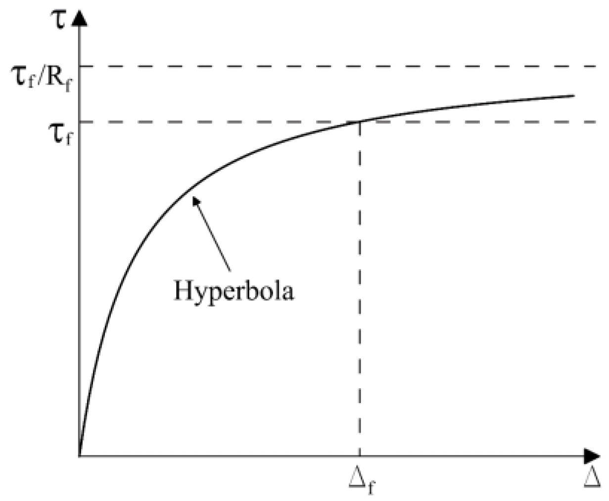
Equation (1) can be viewed as a reciprocal formulation of the local safety factor FSi at the base of the soil block (or slice) i:
FSi = τf i / τi
The initial shear stiffness kinitial is given as a power function of effective normal pressure, proposed in [40]:
Kinitial = K ● G ● (σ'n / Pa)n
K: initial shear stiffness number (dimensionless)
Pa: atmospheric pressure (= 101.3 kPa)
G: reference shear stiffness (= 101.3 kPa/m)
n: pressure dependency exponent
2.2. Multi-Wedge Failure Mechanism
Figure 2 shows the multi-wedge failure mechanism used in this study. It extends the classical two-wedge (bi-linear) model long applied to steep engineered slopes, including mechanically stabilized walls and geosynthetic-reinforced slopes with rigid or near-vertical facings. The enhanced formulation in [21] consists of two active wedges (Wedges 1 and 2), a facing column, and, when present, a passive wedge beneath the toe. This configuration clarifies the role of the facing system in overall stability, and its benefits are further realized when integrated with the FFDM, which supports displacement-based performance evaluation.
Figure 2.
The multi-wedge failure mechanism.
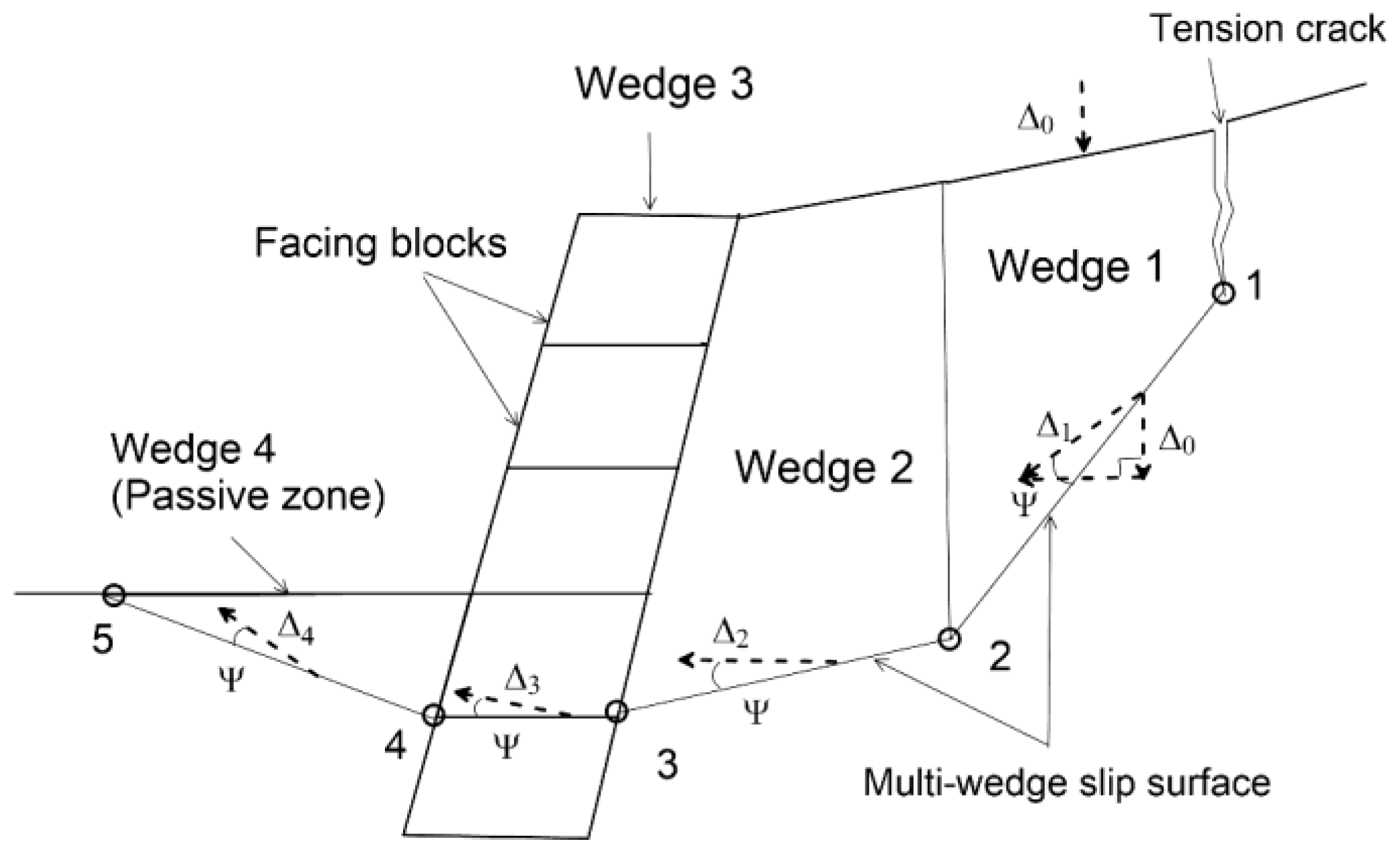
Figure 3 presents the body forces and reaction forces acting on a generalized polygon wedge configuration. Triangular wedges, exemplified by Wedges 1 and 4, constitute special cases where the soil strength and reaction forces along one boundary are assumed to be negligible or zero. By applying force equilibrium in both horizontal (x) and vertical (y) directions, the reaction force on the left side of each wedge (Re) can be expressed as:
Re = f (Rb, Rr, Te, Tb, Tr, Ce, Cb,Cr, ϕe, ϕb, ϕr, kh, kv, Qh, Qv)
Where, Cr = c ● lr / FSi , Cb = c ● lb / FSi , Ce = c ● le / FSi
ϕr = tan-1(tan ϕ / FSi), ϕb = tan-1(tan ϕ / FSi) , ϕe = tan-1(tan ϕ / FSi)
Cr, Cb, Ce: cohesive resistance along soil-block interfaces
lr, lb, le: lengths of soil-block interfaces
ϕr, ϕb, ϕe: mobilized friction angles at interfaces
Tr, Tb, Te: reinforcement force at at interfaces
Rr, Rb: reaction forces at interfaces
To determine the reaction force acting on the left side of each wedge in the LEM analysis, the computation proceeds sequentially from wedge 1 to wedge 3 (or wedge 4, if present). A constant safety factor, Fs, is assumed for all wedges, making every term at the right-hand side of the force-equilibrium equation known except the base reaction Rb. Because both horizontal and vertical equilibrium are enforced, the system is statically determinate. The safety factor is updated iteratively, typically starting with Fs = 1.0, and adjusted until the virtual external force Re on the left side of the final wedge becomes negligible.
Figure 3.
Force equilibrium for a generalized wedge.
In this study, the convergence criterion is defined as a residual horizontal force Re < 0.1 kN, evaluated at the left boundary of wedge 3 (or wedge 4 when present). This residual force represents the virtual horizontal force required to maintain force equilibrium in the multi-wedge system. As a first-order approximation, a residual force smaller than about 1% of the total active thrust at the back of the facing is considered sufficiently small to represent an equilibrium state. For the Tanada wall example, the theoretical Mononobe–Okabe seismic active earth pressure coefficient Kae = 0.25 for ϕ = 40˚ and kh = 0.1, giving an estimated seismic active thrust of about 84 kN/m. Using a convergence tolerance of 0.1 kN therefore corresponds to a residual boundary force on the order of 0.1% of the seismic thrust for kh = 0.1. The appropriate convergence criterion for the two-wedge method is not universal across all soil–structure systems, and in some cases the selected tolerance may have a measurable influence on the results. Users are encouraged to perform preliminary calibration to ensure that the chosen convergence threshold is consistent with the objectives and sensitivity requirements of their study.
In the FFDM framework, the same equilibrium relationship is solved, but the safety factor for each soil block (FSi) and the mobilized reinforcement forces (Tr, Tb, Te) vary with displacement (Δi) based on the hyperbolic reinforcement pullout model [41]. The system remains statically determinate, yet FSi is updated continuously based on the displacement field at the block base and along the interfaces. The computation begins by imposing a small vertical displacement at the crest of wedge 1 (Δ0), such as 0.001 m, and proceeds until all equilibrium conditions are satisfied.
2.3. Post-Peak Stress-Displacement Relationship
The post-peak segment of the shear stress–displacement (τ–Δ) curve is represented using the Versoria (Witch of Agnesi) function [42,43], as shown schematically in Fig. 4. To integrate this model efficiently into the overall stress–displacement framework, a normalized local coordinate system (X–Y) is used. The X-axis origin (X = 0) corresponds to the peak shear stress τf, and the Y-axis origin (Y = 0) corresponds to the asymptotic residual stress τr. Although the Versoria curve reaches τr only at infinite displacement, a finite displacement Δr observed experimentally at the onset of the residual state (X = 1) provides an accurate approximation, typically within 1%. The post-peak shear strength τpost-peak is then expressed as:
τpost-peak = τf -τf ● (t - Y ) = τf ● (1- t + Y )
Y = t3 / ( t2 +X2 )
X= (Δ - Δf ) / (Δr - Δf )
t = (τf -τr ) / τf
Δr = Δf ● Δratio
t: normalized strength reduction between peak and residual states
Y: normalized post-peak shear stress
X: normalized post-peak shear displacement
Δf: shear displacement at peak stress state
Δr: shear displacement at the entrance of residual state
Δratio: residual-to-peak displacement ratio
Figure 4.
A transformed coordinate system of the ‘Versoria’ curve for post-peak stress-displacement relationships.
Figure 4.
A transformed coordinate system of the ‘Versoria’ curve for post-peak stress-displacement relationships.
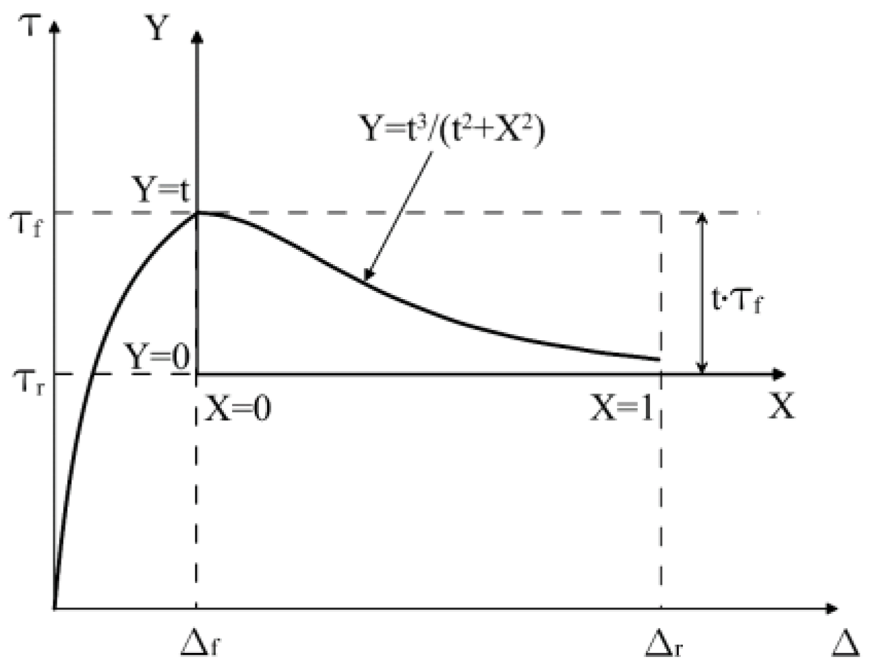
When the post-peak state is considered in the FFDM analysis, Eq. (6) is applied to update the available soil strength along the slip surface whenever the condition Δ > Δf is detected during the iterative displacement computations.
2.4. Displacement Compatibility
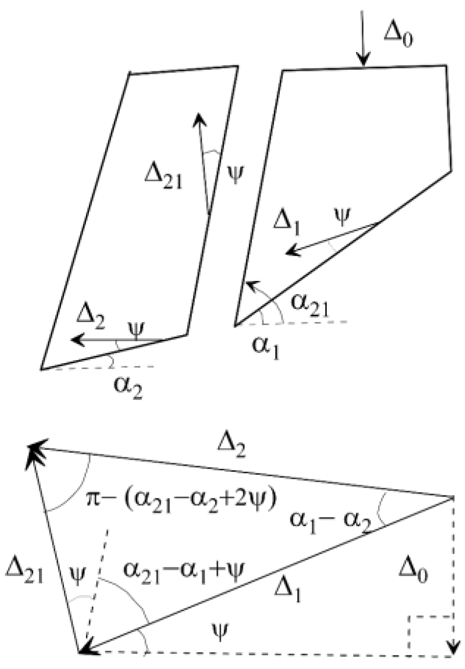
A hodograph (displacement diagram) that satisfies displacement compatibility is shown in Fig. 5. This construction preserves compatible displacements across all soil interfaces and provides the basis for the kinematic analysis of the sliding-block system [44]. The displacement of soil wedge i (Δi) can be expressed as functions of αi (wedge-base inclination angle) and Ψ (dilation angle):
Δi = Δ0 ● f (αi)
f (αi) = cos (α1 -2Ψ) /[sin (α1 -Ψ) ● cos ( 2Ψ- α1)]
Figure 5.
Displacement compatibility of adjacent soil blocks.
2.5. Displacement Increment
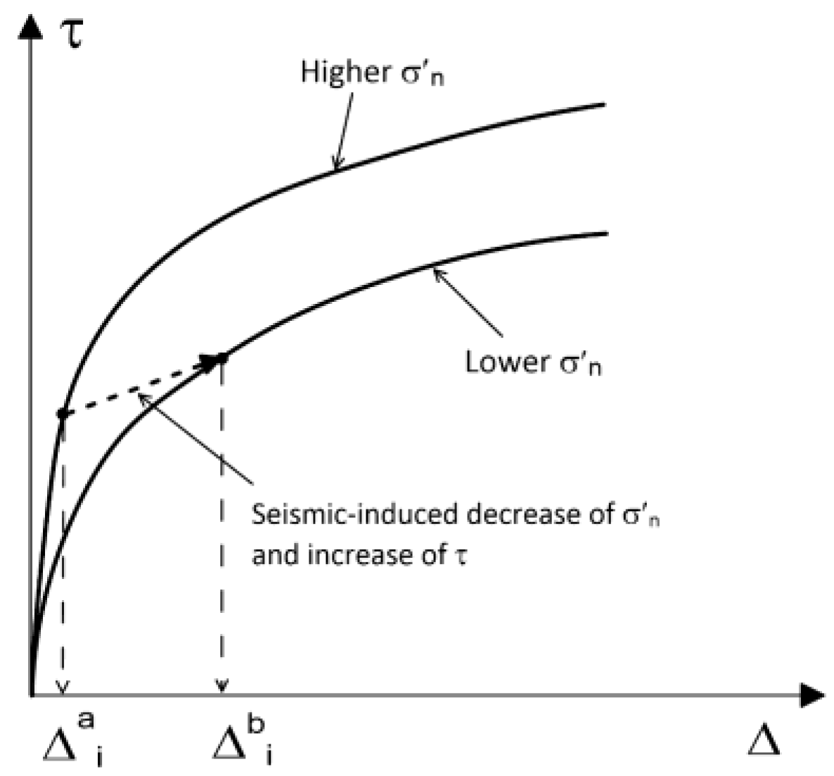
To evaluate slope displacements caused by changes in external or internal conditions—such as seismic loading, water-table fluctuations, or pore-pressure variation—two displacement values are computed for each slice (Δᵢ): one before the event and one after. The displacement increment for slice i, induced by the change in stress conditions, is illustrated schematically in Fig. 6 and defined as:
Δi = Δbi - Δai
Figure 6.
Schematic stress path in response to seismic-induced stress changes.
2.6. The Tanada Wall
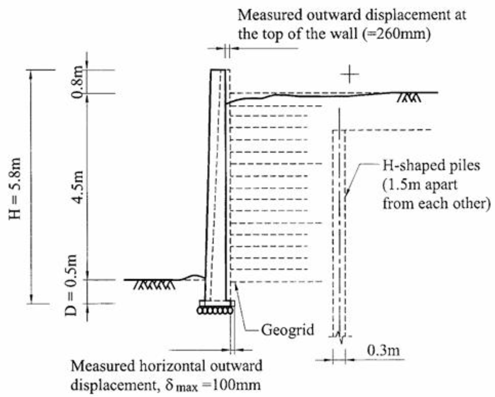
The Tanada wall is a geosynthetic-reinforced soil retaining wall with a full-height rigid panel facing (GRS-FHR), also known as a RRR wall. It formed part of a railway embankment located in a severely shaken area during the 1995 Hyogoken-Nambu earthquake (sometimes referred to as the Kobe earthquake; ML = 7.2). Despite severe damage to nearby houses and soil-retaining structures, the Tanada wall demonstrated high seismic resistance, with observed horizontal displacements of 0.1 m at the toe (i.e., observed Δ3h= 0.1 m) and 0.26 m at the top, as illustrated in Fig. 7. The horizontal displacement of 0.26 m observed at the top of the wall is not included in the comparison because the multi-wedge mechanism adopted here does not capture the additional movement associated with overturning of the facing. Comprehensive post-earthquake investigations and analyses were conducted in [45,46]. Based on site observations, the horizontal peak ground acceleration (HPGA) in the vicinity of the Tanada wall was estimated to be approximately 0.8 g in [45] (where g denotes gravitational acceleration).
Figure 7.
Cross-section of the Tanada wall following the earthquake [45].
Figure 7.
Cross-section of the Tanada wall following the earthquake [45].
2.7. Material Properties
The material properties used in the FFDM analyses of the Tanada Wall are summarized in Table 1. Key considerations for the primary input parameters influencing seismic displacements are as follows:
- Soil strengths (c, φ): The Tanada Wall was constructed using high-quality, cohesionless backfill (cpeak = 0), with a peak internal friction angle of φpeak = 42° obtained from triaxial compression tests [47]. Previous studies comparing φpeak measured under triaxial and plane-strain conditions [48] indicate that the plane-strain friction angle is approximately 1.11 to 1.14 times the triaxial value for Toyoura sand in loose and dense states, respectively. Based on these findings, adopting φpeak = 40° as the design friction angle for the Tanada Wall is slightly conservative and corresponds to the upper bound of recommended design values [49]. In the hyperbolic soil model, φ = 40° is therefore used as an operational value. For post-peak displacement analysis, a higher friction angle of φpeak = 45° (approximately 1.12 times φ = 40°) is applied to represent the plane-strain condition of the railway embankment. Cohesion remains zero in the post-peak range, and the residual friction angle is taken as φres ≈ 0.9 φpeak.
- Displacement-dependent reinforcement pullout model: Mobilized reinforcement forces at the soil–block interface follow the hyperbolic pullout model in [41]. Peak adhesion is cs–r = 0, and the interface friction angle is φs–r = 40°, consistent with geogrids with woven junctions. Model parameters from a pullout test database [52] include stiffness Kt = 10, stress-dependency exponent nt = 0.1, and strength ratio Rt = 0.7.
- Tie-break strength of reinforcement: The tie-break strength Ttie-break = 30 kN/m is taken as the unfactored ultimate tensile strength (Tult) of the geogrid, reflecting high construction quality. This differs from the factored allowable tensile strength (Tallow) commonly used in LEM-based methods.
- H-piles behind the wall: The H-piles, spaced at 1.5 m, were excluded from the analysis. Owing to their slender geometry, wide spacing, and shallow embedment, they provide only negligible resistance to lateral earth pressures.
- Inter-block strength ratio: The inter-block strength ratio (finter-block), defined as the ratio of full shear strength to the shear strength available at block interfaces, is set to 1.0. This reflects the high-quality backfill and the absence of tension cracks observed at the crest after the earthquake.
Figure 8 presents an example of the stress–displacement curves visualized with integrated pre-peak and post-peak parameters (ϕpeak= 45°, φᵣₑₛ = 41° , Δᵣ/Δf = 5.0, K = 400, n= 0.4, Rf= 0.83) as summarized in Table 1. For reference, the experimental data reported in [14] from direct shear tests on dense, remolded Chi-Chi sand—classified as SW-SM under the Unified Soil Classification System (USCS)—are also included.
Figure 9 illustrates the visualized hyperbolic pullout curves for reinforcement ( cs-r= 0, ϕs-r= 40°, Ttie-break= 30 kN/m, Kₜ = 10, nₜ= 0.1, and Rₜ= 0.7). For comparison, experimental pullout data for woven geogrids embedded in recycled construction material classified as SM (USCS), as reported in [53], are also shown. It is observed that the theoretical curves exhibit a stronger dependence on confining pressure than the experimental results, likely because the tests were conducted under relatively low confining pressures (10 and 25 kPa), where material uncertainties and measurement errors tend to have relatively large effects.
2.8. FFDM Displacement Analysis
In the Type-4 (multi-wedge) FFDM analysis implemented in SLOPE-ffdm 2.0, a total of 5,389 trial-and-error facing surfaces is generated to identify critical failure mechanisms characterized by the minimum safety factor (Fs) and the maximum vertical displacement at the slope crest (Δ₀), for a specified pseudo-static seismic coefficient kh (= HPGA/g; g: gravitational acceleration). For the critical failure mechanism, the horizontal displacement of facing (Δ3h) is calculated using Eq. (9). Figure 10 presents the initial configuration of the multi-wedge analysis for the Tanada wall, including the trial-and-error search grids for wedge points 1, 2, and 3. Wedge point 1 defines the right boundary of the multi-wedge, with its trial positions located along the grid at the slope crest. Wedge point 2 represents the base of the triangular wedge and is assigned trial positions in both the x- and y-directions. In this example, wedge point 3 is fixed at the heel of the rigid facing panel because the slip surface is not expected to propagate through the reinforced-concrete facing. Once the analysis begins, trial facing surfaces are systematically generated by connecting all grid-point combinations in the sequence point 3 →2→ 1 (inner →outer loop), as illustrated in Figure 11.
Upon completion of the search, the resulting critical failure mechanisms are displayed in Figure 12. The corresponding failure modes of the reinforcing layers associated with the critical failure surface are also shown in Figure 12, where the symbol “×” denotes tie-break failure and “→” denotes pullout failure.
3. Results
Figure 13 shows the analytical result of FFDM analysis using the multiwedge method (or Type-4 analysis). In this figure, “Low” and “High” soil strength refer to ϕ= 40˚ and 45˚, respectively, listed in Table 1. Every data point in the figure represents a critical (or maximum) value of facing displacement found in trial-and-error multiwedge searches. All curves exhibit consistent response to the increase of input HPGA/g in the range of 0.0 - 0.85. In the case ϕ= 40˚ and hyperbolic soil behavior, the response curves exhibit rapid increases in facing displacement at HPGA ≈ 0.5g. When the post-peak model is considered in the analysis, the response curves show a clear tendency toward failure state at HPGA/g ≈ 0.7 - 0.8. In general, the curves with K= 400 and high soil strength effectively simulate the observed seismic displacement of the Tanada wall, regardless of the incorporation of post-peak strength. This result verifies not only the earthquake-resisting capacity of the Tanada wall but also the capability of SLOPE-ffdm 2.0 in calculating seismic displacements of geosynthetic-reinforced soil retaining walls. It is also noted that the calculated slope displacements span a wide range between 10⁻³ to 10⁻¹ m in response to small to major earthquake intensities. This range highlights both their engineering significance and the accuracy of the program's computational scheme.
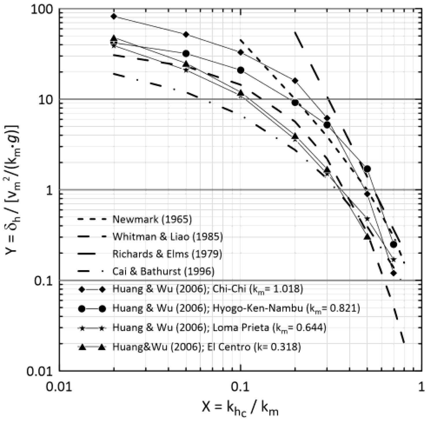
To evaluate the effectiveness of the FFDM relative to hybrid Newmark-type methods, conventional limit-equilibrium slope stability analyses were conducted to develop Fs–kh curves for φ = 40° and φ = 45°, using soil, reinforcement, and facing parameters consistent with those employed in the displacement analyses. The corresponding critical horizontal seismic coefficients are khc = 0.367 for φ = 40° and khc = 0.528 for φ = 45°. Fig. 13 shows normalized seismic displacement versus khc/km relationships (km = HPGA/g) reported in several studies [1,54,55,56,57]. Among these, the relationships derived in [57] from the 1999 Chi-Chi, 1995 Hyogo-ken Nambu, and 1989 Loma Prieta earthquakes, are adopted to estimate the seismic displacement δh of the Tanada Wall. The results are summarized in Table 2 and Table 3 for φ = 40° (khc = 0.367) and φ = 45° (khc = 0.528), respectively. For φ = 40°, the estimated Δ3h range from 0.029 to 0.246 m- an approximately 8-fold variation - which nevertheless brackets the observed Δ3h of 0.1 m . This agreement, however, is contingent upon using operational soil and reinforcement strengths in the LEM-based determination of khc. In contrast, for φ = 45° and km = 0.528, the estimated Δ3h of 0.011 to 0.028 m significantly underestimates the actual wall movement.
Figure 12.
Seismic resistance curves for Tanada wall.
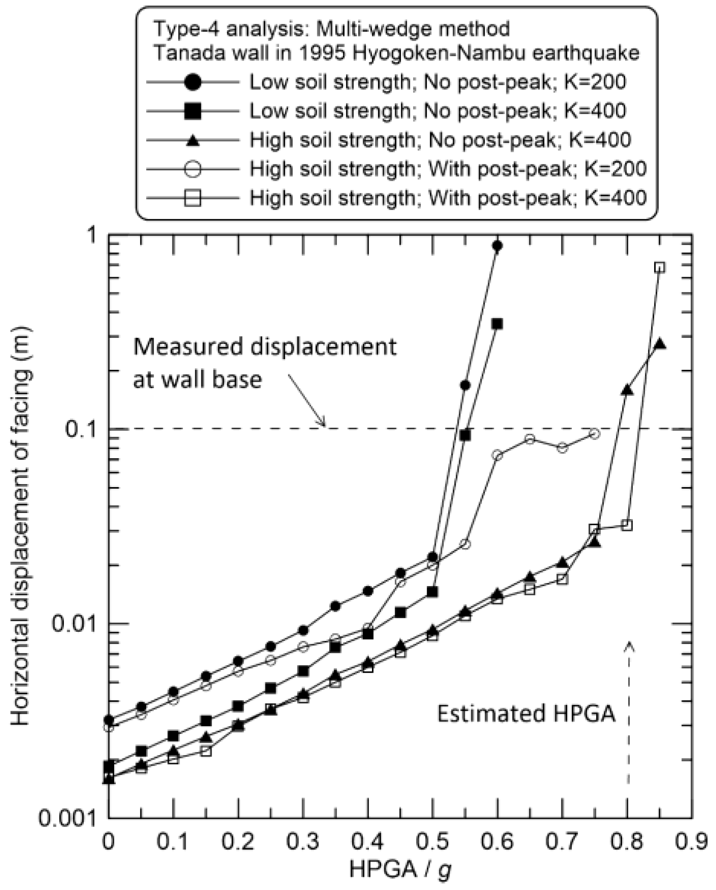
Figure 13.
Normalized seismic displacement vs yield acceleration, compiled from [58].
Figure 13.
Normalized seismic displacement vs yield acceleration, compiled from [58].
4. Discussion
(1) Incorporation of peak and post-peak soil behavior: The FFDM explicitly accounts for both peak soil strength and its post-peak degradation along the slip surface. This avoids the trial-and-error process required to estimate “operational” strength parameters in LEM-based displacement analyses and provides a more consistent basis for evaluating seismic deformation in soil and reinforced soil systems.
(2) Direct use of peak ground acceleration: The FFDM directly uses HPGA/g as its input, thereby capturing the dominant inertial force associated with strong shaking and reducing uncertainty related to the selection of seismographic records. A limitation is that FFDM reflects only the peak acceleration and does not explicitly incorporate frequency content, duration, or spectral characteristics. Even so, the pseudo-static FFDM framework is conceptually analogous to monotonic pushover analysis in structural engineering [59,60], where displacement–kh curves serve a role similar to base-shear–drift relationships used to estimate displacement demand. In this sense, the present study represents an initial attempt to characterize the displacement demand of soil structures using an approach that parallels established practices in seismic performance assessment of reinforced concrete frames [58,59,60] .
(3) Limitations of Newmark-type methods in pre-earthquake assessments: When ground motions are recorded near the site, the LEM-based Newmark approach can reasonably estimate seismic displacements, provided soil and reinforcement strengths are well characterized. In pre-earthquake evaluations, however, the wide range of possible ground motions leads to large variability in predicted displacements, reducing the method’s usefulness for engineering judgment.
(4) Contrasting complexity of soil parameters and seismic inputs: The Newmark approach uses simplified soil strength parameters (c and φ) but requires detailed ground-motion inputs such as period characteristics, maximum velocity, and HPGA. In contrast, the FFDM employs a richer set of soil deformation parameters (c, φ, K, n, Rf) while using a simplified seismic input dominated by HPGA. This inversion of complexity reflects the more mechanistic nature of the FFDM.
(5) Displacement compatibility within the sliding mass: Most Newmark-type methods idealize the sliding mass as a rigid block and do not enforce displacement compatibility among internal components. This simplification contradicts fundamental kinematic requirements and limits the realism of predicted deformation patterns. The FFDM explicitly enforces displacement compatibility which is a core requirement in continuum mechanics and forms the basis of upper-bound plasticity solutions [7,44], improving the internal displacement field of the sliding mass and providing a pathway for refining the accuracy of displacement predictions.
(6) Selection and development of input parameters: The need to select input parameters is unavoidable in all analytical approaches, including Newmark-type methods and FFDM. The results in this study demonstrate how appropriate parameter selection can be achieved. Because FFDM is relatively new, parameter ranges for K, n, and Rf are still developing. A preliminary database has been established by the author [51,52] to support more objective parameter selection, and its refinement will continue as additional case histories become available.
(7) Parametric evaluation and model robustness: Using representative soil parameters for the Tanada Wall backfill, the FFDM produced seismic-resisting curves consistent with observed post-earthquake performance. Extreme parameter combinations, including upper and lower bounds of soil strength and dilatancy angle, were also examined and yielded trends consistent with expected behavior. While a full sensitivity and uncertainty analysis for all parameters (K, n, Rf, Δr/Δf, etc.) lies beyond the scope of this study, it remains an important direction for future research.
(8) Transition from pre- to post-earthquake displacement evaluation: The FFDM overcomes several limitations of Newmark-type methods by enforcing force and moment equilibrium and by accounting for block–block interaction within the failure mass. This enables a seamless transition from static to pseudo-static displacement computation and avoids the common issue in Newmark analyses where pre-yield displacements are ignored. The computational effort is comparable to that of conventional LEM-based factor-of-safety calculations, making FFDM suitable for routine engineering applications. Its limitations primarily relate to the need for deformation-related parameters, for which broader empirical databases are still being developed.
(9) Capability for back analysis and parameter calibration: Although demonstrated only indirectly in this study, the consistent trends of the kh–Δ3h curves in Fig. 12 suggest that back analysis is feasible even for small to moderate earthquake events that generate only minor wall displacement. Previous studies have shown that FFDM-based back analyses for rainfall-induced slope movements can be successfully implemented [37,38]. For the slope subjected to an seismic intensity of HPGA and with a seismic-induced displacement of Δ3h, the back-analysis procedure may follow these steps: (a) back-calculate c and φ using LEM-based slope stability analysis; (b) identify likely values for parameters with limited influence on seismic displacement (n and Rf) based on established databases and material properties; (c) construct K–Δ curves using the calibrated parameters and a constant kh = HPGA/g; (d) determine the calibrated K value from the intersection of the K–Δ3h curves with the observed Δ3h corresponding to a given HPGA; and (e) select the most probable K value based on the existing database. The efficiency of this back-analysis framework can be further enhanced by incorporating machine learning techniques and a performance-based evaluation database for soil retaining walls, following the approach described in [61].
5. Conclusions
This study, implemented through the SLOPE-ffdm 2.0 program, establishes a displacement-based framework for evaluating the seismic performance of geosynthetic-reinforced slopes using the Force-Equilibrium Finite Displacement Method (FFDM). A performance-based re-evaluation of the Tanada Wall, which experienced intense shaking during the 1995 Hyogoken-Nambu earthquake (ML= 7.2), further validates the effectiveness of the method. The results show that using seismic coefficients derived directly from peak ground acceleration eliminates a major source of uncertainty associated with selecting representative seismographs and captures the governing inertial demand at the moment of horizontal peak ground acceleration (HPGA).
The study demonstrates that the FFDM, as implemented in SLOPE ffdm 2.0, provides a robust and practical framework for performance-based seismic evaluation of geosynthetic-reinforced slopes and walls with rigid facings. The seismic-resisting curves produced by the FFDM exhibit a form and interpretive clarity similar to pushover curves widely used in structural engineering, reinforcing that this approach is conceptually aligned with established performance-based methodologies. Its ability to integrate soil behavior, reinforcement interaction, and seismic demand in a displacement-based manner represents a significant advancement over traditional methods.
The comparison with the conventional LEM-based Newmark sliding-block method highlights the advantages of the FFDM. The Newmark approach relies on simplified soil strength parameters and requires consideration of highly variable ground-motion characteristics, often leading to large variability in predicted displacements. In contrast, the FFDM incorporates a richer set of soil deformation parameters while relying solely on HPGA as the seismic input, resulting in more transparent and physically grounded predictions.
One of the advantages of the FFDM is its capability for back-analysis. For structures that experience only small displacements (on the order of several 10⁻³ m) during small-moderate earthquakes, the FFDM can be used to back-calculate soil strength and deformation parameters. These identified parameters can then be applied to predict structural response under more severe shaking. The Newmark-based approach does not offer this capability because its inherent uncertainties make reliable back-analysis impractical.
References
- Newmark, N.M. (1965). Effects of earthquakes on dams and embankments. Geotechnique 1965, 15, 139-160.
- Chang, C.-J., Chen, W.-F., Yao, J.T.P. Seismic displacements in slopes by limit analysis. Journal of Geotechnical Engineering, 1984, 110 (7), 860-874.
- Aminpoor, M.M. and Ghanbari, A. Design charts for yield acceleration and seismic displacement of retaining walls with surcharge through limit analysis. Structural Engineering and Mechanics, 2014, 52 (6), 1225- 1256.
- Shinoda, M. Seismic stability and displacement analyses of earth slopes using non-circular slip surface. Soil and Foundations, 2015, 55 (2), 227-241.
- Kokusho, T., Mori, J., Mizuhara, M., Fang, H. Energy-based newmark method for seismic slope displacements revisited. Soil Dynamics and Earthquake Engineering, 2022, 162, 107449, 1-9.
- Zhang, Y., Xiang, C., Yu, P., Zhao, L., Zhao, J.X., Fu, H. Investigation of permanent displacements of near-fault seismic slopes by a general sliding block model. Landslides, 2022, 19, 187-197.
- Jing, P., Zheng, w., Li, L., Ning, B., Lu, M., Yang, Q., Nan, Y., Li, J., Xu, Y., Liu, J. Seismic slope permanent displacement calculation based on improved Newmark model using upper bound solution of plastic mechanics. Scientific Reports, 2025, 15, 11991, 1-22. [CrossRef]
- Stamatopoulos, C. Sliding system predicting large permanent co-seismic movements of slopes. Earthquake Engineering and Structural Dynamics, 1996, 25, 1075-1093.
- Chopra, A.K., Zhang, L. Earthquake-induced base sliding of concrete gravity dams. Journal of Structural Engineering, 1991, 117 (12), 3698- 3719.
- Rathje, E.M., Bray, J.D. Nonlinear coupled seismic sliding analysis of earth structures. Journal of Geotechnical and Geoenvironmental Engineering, 2000, 126 (11), 1002- 1014.
- Cascone, E., Rampello, S. Decoupled seismic analysis of an earth dam. Soil Dynamics and Earthquake Engineering, 2003, 23, 349-365. [CrossRef]
- Noorzad, R., Omidvar, M. Seismic displacement analysis of embankment dams with reinforced cohesive shell. Soil Dynamics and Earthquake Engineering. 2010, 30, 1149-1157. [CrossRef]
- Feng, W., Lu, Z., Yi, X., Dong, S. A dynamic method to predict the earthquake-triggered sliding displacement of slopes. Mathematical Problems in Engineering, 2021, Article ID 4872987, 1-11. [CrossRef]
- Kramer, S.L., Matthew, W.S. Modified Newmark Model for seismic displacement of compliant slopes. Journal of Geotechnical and Geoenvironmental Engineering, 1997, 123(7), 635-644.
- Beikae, M. Is Newmark method conservative?. Fourth International Conferences on Recent Advances in Geotechnical Earthquake Engineering and Soil Dynamics. 2001, Paper No. 5.16, 1-6.
- Leshchinsky, B.A. Nested Newmark model to calculate the post-earthquake profile of slopes. Engineering Geology, 2018, 233, 139-145.
- Kokusho, T. Spring-supported Newmark model calculating earthquake-induced slope displacement. Journal of Geotechnical and Geoenvironmental Engineering, ASCE, 2024, 150(5), 04024024, 1-13. [CrossRef]
- Song, J., Lu, Z., Pan, Y., Ji, J., Gao, Y. Investigation of seismic displacements in bedding rock slopes by an extended Newmark sliding block model. Landslides, 2024, 21, 461-477.
- Cai, Z., Bathurst, R.J. Seismic-induced permanent displacement of geosynthetic reinforced segmental retaining walls. Canadian Geotechnical Journal 1996, 33(6): 937-955.
- Zeng, X., Steedman, R.S. Rotating block method for seismic displacement of gravity walls. Journal of Geotechnical and Geoenvironmental Engineering, 2000, 126 (8), 709-717.
- Huang, C.-C., Chou, L.H. and Tatsuoka, F. Seismic displacements of geosynthetic-reinforced soil modular block walls. Geosynthetics International 2003, 10 (1), 2-23.
- Li, X., He, S., Wu, Y. Seismic displacement of slopes reinforced with piles. Journal of Geotechnical and Geoenvironmental Engineering, 2010, 136 (6), 880-884.
- Pan, X., Jia, J., Ju, S. A mindlin-based improved Newmark method for the seismic stability of anchored slopes with group anchor effects. Buildings, 2025, 15, 1242, 1-28. [CrossRef]
- Conti, R., Viggiani, G.M.B., Cavallo, S. A two-rigid block model for sliding gravity retaining walls. Soil Dynamics and Earthquake Engineering, 2013, 55, 33-43. http://dx.doi.org/10.1016/j.soildyn.2013.08.007.
- Song, J., Fan, Q., Feng, T., Chen, Z., Chen, J., Gao, Y. A multi-block sliding approach to calculate the permanent seismic displacement of slopes. Engineering Geology, 2019, 48-58. [CrossRef]
- Bandini, V., Biondi, G., Cascone, E., Rampello, S. A GLE-based model for seismic displacement analysis of slopes including strength degradation and geometry rearrangement. Soil Dynamics and Earthquake Engineering, 2015, 71, 128-142. http://dx.doi.org/10.1016/j.soildyn.2015.01.010.
- Cui, Y., Liu, A., Xu, C., Zheng, J. A modified Newmark method for calculating permanent displacement of seismic slope considering dynamic acceleration. Advances in Civil Engineering, 2019, Article ID 9782515, 1-10. [CrossRef]
- Ji, J., Wang, C.-W., Cui, H.-Z., Li, X.-Y., Song, J., Gao, Y. A simplified nonlinear coupled Newmark displacement model with degrading yield acceleration for seismic slope stability analysis. International Journal of Numerical and Analytical Methods in Geomechanics, 2021, 45, 1303-1322. [CrossRef]
- Le, P.H., Nishimura, S., Nishiyama, T., Nguyen, T.C. Modified Newmark approach for evaluation of earthquake-induced displacement of earth dam- Applying for re-division of sliding mass. International Journal of GEOMATE, 2021, 21 (86), 1-8. [CrossRef]
- Ji, J., Lin, Z., Li, S., Song, J., Du, S. Coupled Newmark seismic displacement analysis of cohesive soil slopes considering nonlinear soil dynamics and post-slip geometry changes. Computers and Geotechnics, 2024, 174, 106628, 1-15. [CrossRef]
- Nguyen, V.B., Jiang, J.-C., Yamagami, T. Modified Newmark analysis of seismic permanent displacements of slopes, Landslides, 2005, 41 (5), 458-466.
- Doolin, D.M., Sitar, N. Displacement accuracy of discontinuous deformation analysis method applied to sliding block. Journal of Engineering Mechanics, 2002, 128 (11), 1158-1168. [CrossRef]
- Goldgruber, M., Shahriari, S., Zenz, G. Dynamic sliding analysis of a gravity dam with fluid-structure-foundation interaction using finite elements and Newmark's sliding block analysis. Rock Mechanics and Rock Engineering, 2015, 48, 2405-2419. [CrossRef]
- Ibrahim, K.M.H.I. Seismic displacement of gravity retaining walls. HBRC Journal, 2015, 11, 224-230. [CrossRef]
- Song, J., Lu, Z., Ji, J., Gao, Y. A fully nonlinear coupled seismic displacement model for earth slope with multiple slip surfaces. Soil Dynamics and Earthquake Engineering, 2022, 159, 107353, 1-13. [CrossRef]
- Huang, C.-C. Developing a new slice method for slope displacement analyses. Engineering Geology, 2013, 157, 39-47.
- Huang, C.-C. Back-calculating strength parameters and predicting displacements of deep-seated sliding surface comprising weathered rocks. Int. J. of Rock Mechanics and Mining Sciences 2016, 88, 98-104.
- Lo, C.-L., Huang, C.-C. Groundwater-table-induced slope displacement analyses using different failure criteria, Transportation Geotechnics 2021, 26, 100444.
- SLOPE-ffdm 2.0: Computer programs for slope stability and displacement analyses using Force-equilibrium-based Finite Displacement Method (FFDM), 2025. Available online: https://slope.it.com/.
- Duncan, J.M. and Chang, C.Y. Nonlinear analysis of stress and strain in soils. J. Soil Mechanics and Foundation Division, ASCE 1970, 96 (SM5), 1629-1653.
- Huang, C.-C. Force equilibrium-based finite displacement analyses for reinforced slopes: Formulation and verification. Geotextiles and Geomembranes 2014, 42, 394-404.
- Lawrence, J. D. Witch of Agnesi. In A Catalog of Special Plane Curves; Dover Publications: New York, USA, 1972; pp. 20–23.
- Lo, C.-L., Huang, C.-C. Displacement analyses for a natural slope considering post-peak strength of soils. GeoHazards 2021, 2, 41-62.
- Atkinson, J.H. An introduction to the mechanics of soils and foundations.; McGraw-Hill: Berkshire, England, 1993; McGraw-Hill, London. 215-239.
- Tatsuoka, F., Koseki, J., Tateyama, M., Munaf, Y. and Horii, K. Seismic stability against high seismic loads of geosynthetic-reinforced soil retaining structures. Keynote Lecture, 6th Int. Conf. on Geosynthetics, Atlanta, USA. 1998, 103-142.
- Huang, C.-C. and Wang, W.-C. Seismic displacement of a geosynthetic-reinforced wall in the 1995 Hyogo-Ken Nambu earthquake. Soils and Foundations, 2005, 45 (5), 1-10.
- Tateyama, M. Back analyses of damaged retaining structures for railway by Hyogoken-Nambu earthquake. RTRI Report, 1996 , 10 (12). 11-16 (in Japanese).
- Tatsuoka, F., Pradhan, T., Lam, W.K., Horii, N.Y. Angle of internal friction of sand by various types of shear tests. Tsuchi Do Kiso, 1987, 35 (12), 55-60. (in Japanese).
- Japan Railway Technical Research Institute. Guidelines for the Design of Railway Structures- Soil Structures. Chapter 5: Reinforced earth. Maruzen, Tokyo, Japan, 1992, 137-162.
- Chiang, Y.-J. Analyses for rainfall-induced slope displacements taking into account various displacement fields and failure criteria. Master thesis, National Cheng Kung University, Tainan, Taiwan, July 2017.(in Chinese).
- Software Development Series 10- Modelling material behavior. Available on-line: https://slope.it.com/product/?goto=product.
- Software Development Series 13- Modelling pullout behavior of reinforcement material. Available on-line: https://slope.it.com/product/?goto=product.
- Vieira, C. and Pereira, P.M. Influence of the geosynthetic type and compaction conditions on the pullout behavior of geosynthetics embedded in recycled construction and demolition materials. Sustainability 2022, 14, 12070.
- Richards, R., Elms, D.G. Seismic behavior of gravity retaining walls. Journal of the Geotechnical Engineering Division, ASCE 1979; 105(GT4):449-464.
- Whitman, R.V. and Liao, S. Seismic design of gravity retaining walls. Miscellaneous Paper GL-85-1, Department of the Army, US Army Corps of engineers 1985, Washington, DC.
- Cai, Z. and Bathurst, R.J. Deterministic sliding block methods for estimating seismic displacements of earth structures. Soil dynamics and Earthquake Engineering 1996, 15(4), 255-268.
- Huang, C.-C. and Wu, S.-H. Simplified approach for assessing seismic displacements of soil-retaining walls. Part Ⅱ: Geosynthetic-reinforced walls with rigid panel facing. Geosynthetics International, 2007, 14 (5), 264-276.
- Kim, S.P., Kurama, Y.C. An alternative pushover analysis to estimate seismic displacement demands. Engineering Structures, 2008, 30, 3793-3807. [CrossRef]
- Yip, C.-C., Marsono, A.K., Wong, J.-Y., Lee, S.-C. Seismic performance of scaled IBS block column for static nonlinear monotonic pushover experimental analysis. Jurnal Teknologi (Sciences & Engineering), 2018, 80 (1), 89-106.
- Gunes, N. Comparison of monotonic and cyclic pushover analyses for the near-collapse point on a mid-rise reinforced concrete framed building. Earthquakes and Structures, 2020, 19 (3), 189-196. [CrossRef]
- Flugione, M., Palladino, S., Esposito, L., Sarfarazi, S., Modano, M. A multi-stage framework combining experimental testing, numerical calibration, and AI surrogates for composite panel characterization, Buildings, 2025, 15, 3900. [CrossRef]
Figure 8.
Integrated pre- and post-peak stress-displacement curves for FFDM analyses.
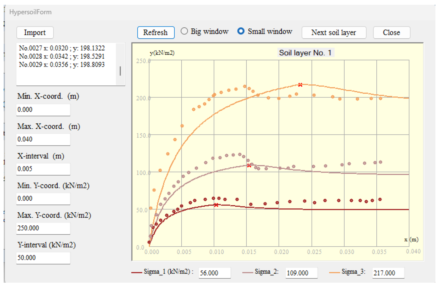
Figure 9.
Stress-displacement curves for reinforcement pullout in the FFDM analyses.

Figure 10.
Initial configuration for the multi-wedge analysis in SLOPE-ffdm 2.0.
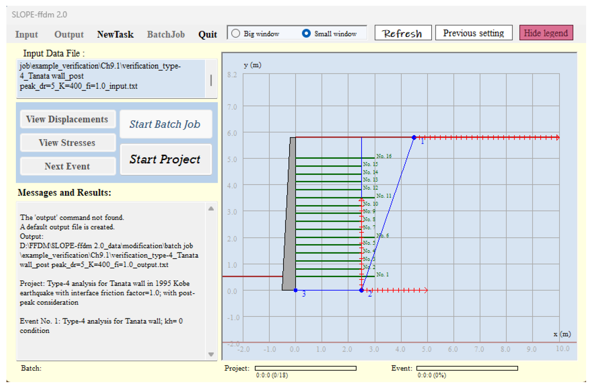
Figure 11.
Trial-and-error search for the critical failure mechanism.
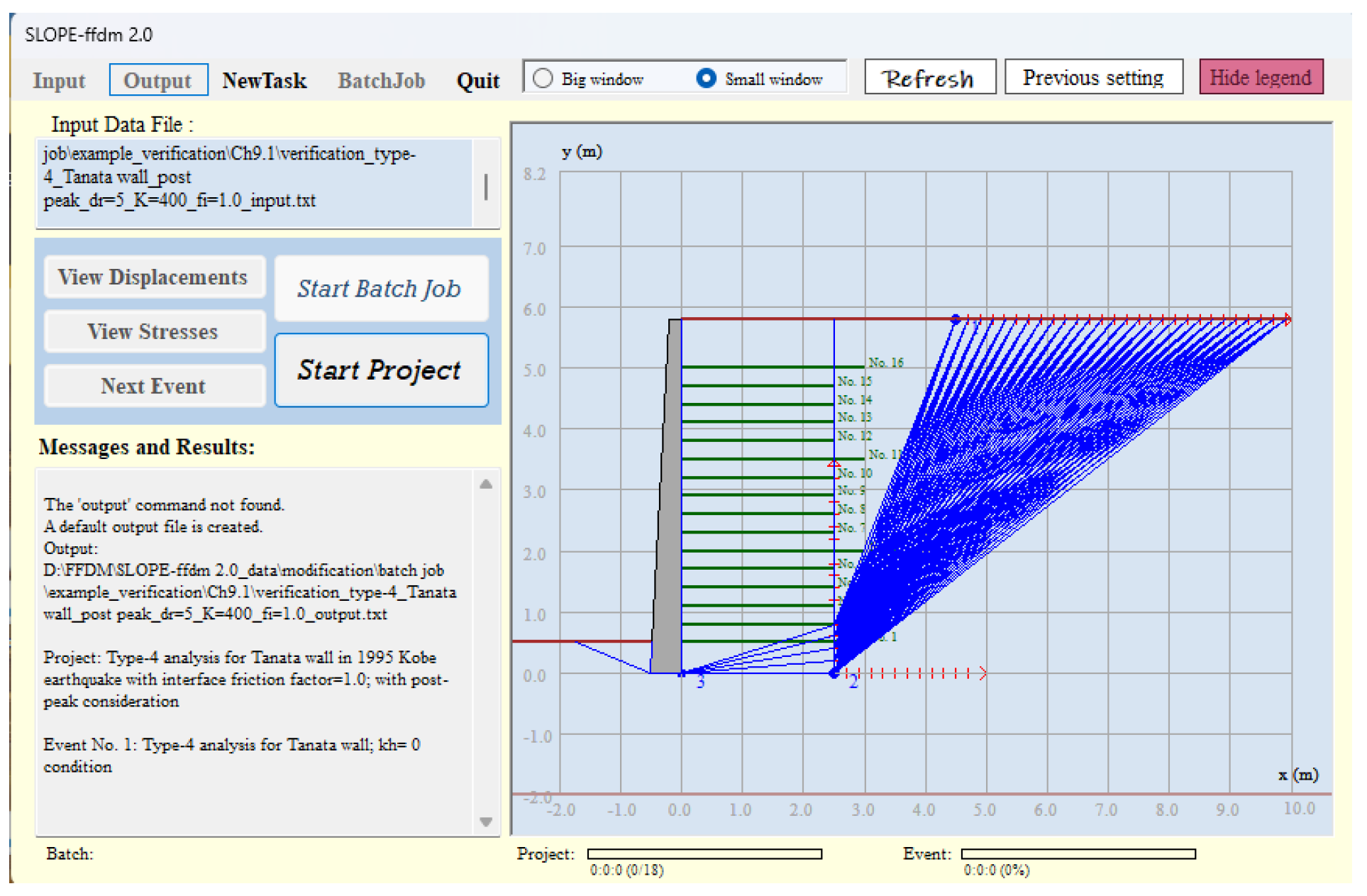
Figure 12.
Critical failure mechanisms identified from the limit-equilibrium and displacement analyses, characterized by the minimum Fs and maximum Δ0.
Figure 12.
Critical failure mechanisms identified from the limit-equilibrium and displacement analyses, characterized by the minimum Fs and maximum Δ0.
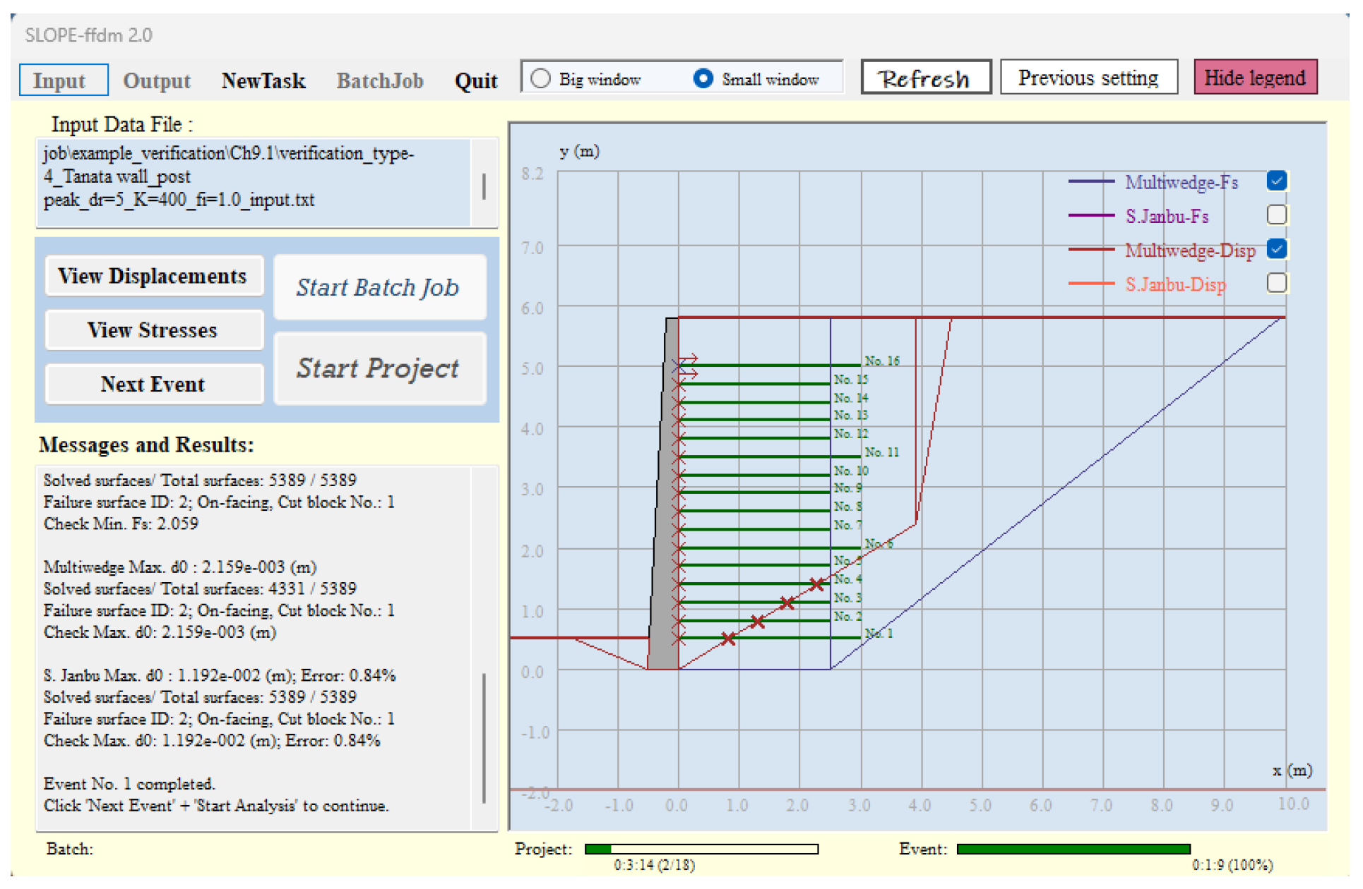

Table 1.
Material properties used in the FFDM analysis for Tanada wall.
| Soil Hyperbolic model |
Reinforcement Hyperbolic pullout model |
Facing-related strength parameters |
|||
| c | 0 kPa | cs-r | 0 | cb-r | - |
| ϕ | 40° | ϕs-r | 40° | ϕb-r | - |
| K | 200, 400 | Kt | 10 | Tconnect | 30 kN/m |
| n | 0.4 | nt | 0.1 | cback | 0 |
| Rf | 0.83 | Rt | 0.7 | ϕback | 30° |
| Ψ | 5° | Ttie-break | 30 kN/m | cbase | 0 |
| ϕbase | 40° | ||||
| Post-peak model | Post-peak model | Post-peak model | |||
| cpeak | 0 | Not available | Not available | ||
| ϕpeak | 45° | ||||
| cres | 0 | ||||
| ϕres | 41° | ||||
| Δr/Δf | 5.0 | ||||
*cs-r, ϕs-r: adhesion and friction angle, respectively, at soil-reinforcement interface *cb-r, ϕb-r: adhesion and friction angle, respectively, at facing block-reinforcement interface. In the case of rigid panel facing, these values are not required. *cback, ϕback: adhesion and friction angle, respectively, at the back-face of facing *cbase, ϕbase: adhesion and friction angle, respectively, at the base of facing. *Ttie-break: tie-break strength of reinforcement. *Tconnect: connecting force at facing-soil interface. This input is exclusively for the case of rigid panel facing which is equal to Ttie-break in this case study of the Tanada wall.
Table 2.
Seismic displacements for Tanada wall estimated using khc= 0.367, km= 0.821.
| Earthquake | X |
Y | vmax (m/s) |
HPGA (g) |
Estimated Δ3h (m) |
| Chi-Chi | 0.446 | 1.5 | 1.28 | 1.018 | 0.246 |
| Hyogo-Ken-Nambu | 0.446 | 2.2 | 0.81 | 0.821 | 0.179 |
| Loma Prieta | 0.446 | 0.6 | 0.552 | 0.644 | 0.029 |
Table 3.
Seismic displacements for Tanada wall estimated using khc= 0.528, km= 0.821.
| Earthquake | X |
Y | vmax (m/s) |
HPGA (g) |
Estimated Δ3h (m) |
| Chi-Chi | 0.643 | 1.7 | 1.28 | 1.018 | 0.028 |
| Hyogo-Ken-Nambu | 0.643 | 0.38 | 0.81 | 0.821 | 0.031 |
| Loma Prieta | 0.643 | 0.22 | 0.552 | 0.644 | 0.011 |
Disclaimer/Publisher’s Note: The statements, opinions and data contained in all publications are solely those of the individual author(s) and contributor(s) and not of MDPI and/or the editor(s). MDPI and/or the editor(s) disclaim responsibility for any injury to people or property resulting from any ideas, methods, instructions or products referred to in the content. |
© 2026 by the authors. Licensee MDPI, Basel, Switzerland. This article is an open access article distributed under the terms and conditions of the Creative Commons Attribution (CC BY) license (http://creativecommons.org/licenses/by/4.0/).
Copyright: This open access article is published under a Creative Commons CC BY 4.0 license, which permit the free download, distribution, and reuse, provided that the author and preprint are cited in any reuse.


