
Submitted:
05 December 2025
Posted:
22 December 2025
You are already at the latest version
Abstract
We develop a framework in which lightcones, $(p,q)$ strings, and M-theory compactifications are equipped with an explicit layer of modal structure. Starting from Minkowski spacetime $\mathbb{M}^4$ with its usual null cones, we consider a background $\mathbb{M}^{4\times 7} = \mathbb{M}^4 \times G_2$ and attach to each spacetime point $\mathfrak{x}$ an internal $G_2$-source fiber. Local field configurations are encoded by propositions in a fuzzy Heyting--Kripke semantics, and a localized action $S(\mathfrak{x})$ defines normalized truth-values $\sigma(\mathfrak{x},\varphi) \in [0,1]$ which we interpret as a ``modal radius'' on a refined lightcone. Nilpotent extensions of the truth-value space capture unphysical ``eternal photon'' modes as purely internal, non-observable directions in the $G_2$-source. On this background we introduce \emph{interstices} $\varcurlywedge = G_2 \cap \mathbb{M}^4$ at $(p,q)$ string junctions, regarded as higher-dimensional analogues of Chan--Paton defects. Each interstice supports a pair of S-dual field-families (FFs) $(\Phi,\Psi)$ with a coprime arithmetic grading that organizes primary, descendant, and auxiliary modes, and we show how a $G_2$-inspired flux superpotential can be reinterpreted as a ``modal'' functional controlling the exponents in $\sigma(\mathfrak{x},\varphi) = n^{-z_i}$. We work out explicit examples: a three-leg $(p,q)$ junction and a minimal two-junction web with an internal $(1,1)$ segment, including concrete numerical assignments for $\sigma(\mathfrak{x},\varphi)$, an S-duality reshuffling of the FFs, and a simple propagation rule for modal data along the internal edge. The resulting picture can be phrased in terms of a small Kripke frame whose accessibility relation is determined by the (p,q) web geometry. Taken together, these constructions suggest that junctions, defects, and compactification data in string/M-theory admit a natural description in terms of modal structure on lightcones, with logical semantics providing a controlled way to track which field configurations are realized, suppressed, or confined to nilpotent internal sectors.
Keywords:
modal logic
; m-theory
; string theory
; lightcones
; g2 manifolds
; compactification
1. Introduction
Classical and quantum field theories have largely been developed on top of classical, bivalent logics. While there are notable exceptions (e.g. the Birkhoff–von Neumann proposal for quantum logic [3], or topos-theoretic approaches to contextuality and measurement [5]) it is still rare for modal or substructural logics to be built directly into the foundations of physical models. Nevertheless, physicists routinely use modal language informally: fields “turn on” or “turn off”, a coupling regime is “accessible” from another, a constraint “forces” or “allows” a certain vacuum, and so on. These phrases hint at an underlying logical and relational structure, but this structure is usually kept in the background as mere metaphor.
One aim of this paper is to bring that background structure to the foreground, by incorporating Kripke–Joyal-style semantics into a concrete physical setting. Very roughly, we regard a family of field configurations as a kind of Kripke frame, where worlds represent dynamical states or background geometries, and accessibility relations encode physically realizable transitions, couplings, or junctions between them. In this view, a statement such as “this field can turn on” corresponds not merely to a yes/no proposition, but to a modal claim about which neighboring configurations are dynamically reachable.
We begin with a simple schematic expression of this idea:
in which a “possible” state for a field is still “off” just before a time t, but at t is instantaneously activated. Here is interpreted as an accessibility relation or update operation at time t, expresses the mere possibility that could be turned on in some accessible configuration, while expresses the stability or necessity of being on throughout a suitable neighborhood (temporal, spatial, or configuration-space) of that update.
The central proposal of this work is that, when we move to the setting of -string junctions, these accessibility relations can be understood as interstitial fields: additional degrees of freedom living not on a single worldsheet or brane, but “in between” them. At a junction of multiple -strings, the compatibility conditions between charges, tensions, and boundary conditions can be organized into a network of possible and necessary configurations. The interstices of this network (the gaps and overlaps between individual strings and their backgrounds) carry auxiliary fields whose behavior is most naturally described in modal terms.
In more concrete terms, we will model a collection of -string junctions as a structured graph or category, whose objects are local configurations and whose morphisms encode admissible deformations, splittings, and recombinations. To each such morphism we associate an accessibility relation of the form , and we interpret interstitial fields as those modes that control, or are controlled by, these relations. The resulting picture is that of a decorated network of junctions, in which logical modalities and physical couplings are blended into a single formalism.
This work should be read as complementary to our earlier investigation of Chan–Paton defects on open strings [6]. There we treated defects as bimodular obstructions on extended objects, generalizing Chan–Paton factors to -bimodules and interpreting pseudoparticles as both physical and semantic obstructions to lifting in braided settings.1 In the present paper we focus instead on interstices in compactified backgrounds and the associated modal field-families (FFs). Interstices are the natural higher-dimensional avatars of Chan–Paton defects; they carry the same obstruction-theoretic flavor, but are now organized by a modal lightcone, fuzzy Heyting–Kripke semantics, and internal -sources, rather than by braids on a single open string.
2. Type IIB String Theory, Dualities, and (p, q)-Strings
In this section, we hope to encapsulate the last half-a-century-or-so worth of string history, in the fashion of a mini-primer. Naturally, many things will be left out, to prevent the length of this paper from spiralling out of control. We will first consider the origins of string theory, and make our way to our topic of interest: -strings in type IIB string theory.
2.1. From Dual Resonance Models to Type IIB (A Very Short History)
String theory did not begin life as a theory of quantum gravity or unification, but as an attempt to model hadronic scattering. In the late 1960s, the S–matrix program sought amplitudes that would exhibit both Regge behavior at high energy and crossing symmetry between different channels. Veneziano’s 1968 four–point amplitude provided a remarkably simple answer: a -function of the Mandelstam variables that produced an infinite tower of narrow resonances lying on approximately linear Regge trajectories and satisfied the desired “duality” between s– and t–channels.2 This construction was soon generalized to N–point “dual resonance models,” whose factorization properties and infinite oscillator–like spectrum suggested that some underlying extended system was being described.
Between 1969 and 1970, Nambu, Susskind, and Nielsen independently proposed that the dual resonance model could be understood as a theory of relativistic strings: one–dimensional objects whose world–sheets sweep out the surfaces underlying Veneziano’s amplitudes. In this picture, the infinite tower of resonances arises from quantized vibrational modes of an open or closed string, and the linear Regge trajectories are explained by a rotating string whose angular momentum grows linearly with its energy. The dual amplitudes acquire a geometric interpretation as correlation functions of a two–dimensional field theory on the string world–sheet, rather than as ad hoc functions engineered to fit scattering data.
2.2. Type IIB, the Axio–Dilaton, and
The original bosonic string theory, however, was clearly incomplete as a fundamental theory: it lived in twenty–six dimensions, contained a tachyonic ground state, and lacked fermions. The next step was to introduce world–sheet fermions and supersymmetry (Ramond, Neveu–Schwarz), and then to impose spacetime supersymmetry in ten dimensions. This led to a family of superstring theories with vastly improved consistency properties, in particular the removal of most tachyonic instabilities and the appearance of fermionic states in the spectrum. A crucial development came in 1984, when Green and Schwarz showed that certain ten–dimensional superstrings are free of gauge and gravitational anomalies via what is now called the Green–Schwarz mechanism.3 Anomaly cancellation and other consistency conditions singled out five perturbative ten–dimensional superstring theories: Type I, Type IIA, Type IIB, heterotic , and heterotic .
Among these, Type IIB quickly emerged as the most natural arena for exploring dualities and extended objects. It is a theory of oriented closed strings with chiral supersymmetry in ten dimensions, a self–dual five–form field strength, and a rich spectrum of D–branes on which open strings can end. Most importantly for our purposes, its low–energy supergravity description exhibits an symmetry acting on the complex axio–dilaton
where is the Ramond–Ramond scalar and is the dilaton. In the full quantum theory this continuous symmetry is broken to the arithmetic group , which acts as a strong–weak duality (alias: S–duality) relating different coupling regimes. Under this duality, the fundamental NS–NS string and the D1–brane transform as a doublet, and more generally one is led to consider bound states carrying a pair of integer charges .
The appearance of an exact acting on , together with a multiplet of –strings and higher–dimensional branes, makes Type IIB a direct descendant of the duality ideas already implicit in the Veneziano amplitude and dual resonance models. In the remainder of this section we recall the basic structure of this symmetry and the role of –strings and junctions, which will serve as the physical stage for the interstitial, modal, and probabilistic structures developed in Section 3.1 and beyond.
2.3. -Strings, Junctions, and Webs as Our Arena
In Type IIB string theory the fundamental NS–NS string (usually denoted F1) and the D1–brane (D1) are not isolated species, but members of a larger multiplet of bound states. The complex axio–dilaton of equation (2) transforms under by fractional linear transformations, and the pair of integer charges —measuring NS–NS and R–R string charge, respectively—transforms as a column vector in the fundamental representation. A –string is, roughly speaking, a BPS bound state carrying p units of F1 charge and q units of D1 charge.4 In a fixed background the tension of such a state is proportional to
so that the action on and on preserves the spectrum of BPS string tensions.
A particularly important feature of Type IIB is that these –strings can meet at junctions. The simplest nontrivial case is a three–pronged junction J, in which three string segments with charges , , and join at a point.5 Charge conservation at the junction requires
so that the total NS–NS and R–R charge is conserved. For a BPS configuration in flat space, the tensions of the three strings must also balance: the vectors with magnitudes and directions along the spatial legs add up to zero. Equivalently, after fixing the complex structure in the plane of the junction, the angles between the legs are determined by the complex numbers ; the three tension vectors form a closed triangle in the complex plane. This picture extends to more elaborate planar –webs (as in [1,13]), in which multiple junctions and string segments are glued together to form a graph whose edges are labeled by charges and whose geometry is constrained by local charge conservation and tension balance.
Such –webs play several roles in the literature: they provide a useful description of BPS states in certain supersymmetric gauge theories, a way of encoding information about 7–brane backgrounds and F–theory compactifications, and a geometric representation of the action of on charges and junctions. For our purposes, the key point is more modest; viz. a –web gives a concrete geometric and kinematic scaffold on which fields can live, and along which excitations can propagate, while the duality group acts nontrivially on the discrete charge labels decorating the edges and junctions.
In subsequent sections we recast these –webs in the modal and algebraic framework of Section 3.1. The individual string segments and junctions will become objects and morphisms in a category of paths and terms, and the regions “in between” them (the interstices of the web) will host auxiliary fields whose activation and propagation are naturally described in modal terms. It is in these interstitial regions, rather than on any single leg alone, that our accessibility relations and formal power series of update operations will live.
3. Modal and Algebraic Aspects
Before we can begin with the real physical panache, let’s begin with a few simple tools we will use. Having explained the relevant history, let us now turn to some simple gadgets we will use. Section 3.1 nods towards some of mine and Emmersons’ previous research, namely [6] and [7]. We will not yet fully engage with them, and inhibit ourselves enough to get out the necessary details only.
3.1. Modal Algebra at a Point on the String
Recall the schematic relation of equation (1) in which a mode that is merely possible just before time t becomes necessary (or stably on) at time t. Let be an open string worldline (or a spatial slice of a worldsheet), equipped with a coordinate . We write points on as , and for each such point choose a small neighborhood
A field configuration along the string will be denoted by , and we allow ourselves to restrict it to this neighborhood:
We imagine that the dynamics provides a family of time-evolution operators
acting on the space of field configurations on , such that is induced by translating by a small time-step .6 For each integer we write
for the n-step iterate.
To connect this with the modal notation, we fix a point and consider the restriction of the time-evolved field to :
The informal statement that the mode “turns on at after n time steps” can then be encoded as an accessibility relation
where the right-hand side is read as: “after n steps, the configuration lies in a state in which is accessible at the point on the string.”
Notation 1.
We distinguish between field configurations, denoted by symbols such as ϕ and ψ, and logical propositions about those configurations, which we denote by φ and ς. The algebra (see again appendix §app:kripke-frames for more details) consists of such propositions (e.g. “ϕ is nonzero on "), and the satisfaction relation should be read with this in mind.
Algebraically, for each fixed , this is realized by a family of local modal operators
acting on a Heyting (or Boolean) algebra of propositions about the behavior of fields in the neighborhood . The update map induces the modality via restriction:
The dual operator encodes stability, in the sense that
In particular, the relation (1) can be read locally at as the statement that
We now enrich this picture with a mild probabilistic decoration. We equip the parameter interval with a probability distribution , normalized so that
One can then think of an open string configuration as a pair
and of a point together with its neighborhood as a localized probe of this weighted interval.
In the closed-string case, we identify the endpoints via , and choose a basepoint . The resulting decorated loop-space can be encoded schematically as
where the decorator (as in [7]) is a (possibly infinite) product of mapping spaces
Here the family of probability marginals
is obtained by rescaling and restricting the base distribution along a poset of scales.
Remark 1.
We will not need the full machinery of these decorated loop-spaces until we discuss junctions and interstices; for the moment, they serve only as a reminder that our local modal operators at can be organized into a richer structured space.
Returning to the open-string case, the contribution of a neighborhood of to the worldsheet action can be isolated by a bump function (alias: characteristic function)
supported in and normalized in such a way that a partition
of unity along satisfies
If denotes the full action of a field configuration along the string, we define the localized action at by
so that, schematically,
The idea, then, is that the action becomes nonzero precisely when the modality has “turned on” the corresponding mode at , in the sense of (5). In this way, the collection of local modal operators
along the string, together with the time-translation monoid generated by , encodes a “modal lightcone” of accessible and realized configurations at each point on .
3.2. Algebraic Aspects and Formal Power Series
We now package the local modal dynamics at a point into a simple algebraic structure. The basic idea is that the iterates of the accessibility relation in (5) generate a monoid of “update operations”, and that formal power series in this monoid encode discrete histories in the modal lightcone of Figure 1.
Throughout this subsection we fix a point and work with the local Heyting (or Boolean) algebra and its modal operators as in (5)–(7). We also fix a commutative coefficient ring
so that formal ℏ-expansions can later be combined with formal modal expansions using deformation quantization, if we are so-inclined.
Definition 1.
The local update monoid at is the free monoid
generated by a symbol corresponding to one forward modal update at . We write for the word of length n, with the empty word.
Concretely, the generator is realized as the one-step local modality
and the canonical representation
sends to the n-fold iterate . In these terms, the future layers of the modal lightcone are indexed by the elements of ; the nodes labeled , , ...in Figure 1 correspond to , , ...acting on the present configuration.
3.2.1. Monoid Rings and Formal Modal Power Series
The first algebraic object associated to is its monoid ring over k:
whose underlying k-module has basis and whose multiplication extends the monoid law . Since is free on one generator, there is a natural identification
sending to and itself to the indeterminate z.
To describe infinite modal histories we pass to the formal completion:
the ring of formal power series in the generator with coefficients in . A typical element of has the form
which we may symbolically rewrite as
Formally, (21) is a k-linear combination of endomorphisms of ; in situations where only finitely many iterates act nontrivially on a given proposition , the right-hand side defines an honest endomorphism of . Intuitively, encodes a weighted sum over all modal futures of , with the coefficient assigned to the n-step layer of the lightcone.
3.2.2. Modal Generating Functionals
The same formalism can be applied to the localized action (14). For a fixed field configuration and point , we may consider the sequence of localized actions along the iterates of the dynamics,
and package them into a formal “modal generating functional’’
with coefficients as in (20). While we will not commit to a specific choice of the weights here, (22) illustrates how the discrete-time evolution in (4) and the localized action in (14) can be organized into a single formal object whose combinatorics is governed by the monoid and whose coefficients live in the deformation ring k.
In this sense, the formal series ring (19) plays the role of a “modal completion’’ of the local dynamics at : it encodes all finite compositions of the basic update, and their ℏ-dependent weights, without requiring any analytic convergence. This is directly analogous to the way formal power series in an operadic or PROP-based field theory keep track of all possible compositions of elementary operations or vertices, independently of analytic issues (see for example the expository discussion in [2] and the operadic frameworks developed in [14,15]).
Remark 2
(Abstract Nonsense). At a more categorical level, one can think of the string γ as living in a product category
where is a (2-)category of paths and homotopies between them,7 and encodes additional physical data such as Chan–Paton factors, background charges, or boundary conditions. A path in , tensored with suitable term data in , becomes a bona fide physical string configuration, and natural transformations in the bi-category represent symmetries or gauge invariances. The local update monoid can then be viewed as a submonoid of the endomorphisms of such an object, generated by a distinguished “one-step’’ update at . We will not develop this categorical picture in detail here, but it provides a natural home for the monoid and power-series structures introduced above, and connects them with the broader operadic and PROP-based approaches to field theory.
3.2.3. Interaction with Probability Weights and Bump Functions
The constructions above separate two kinds of data:
The monoid indexes discrete time-steps in the evolution (4), while the measure and bump determine how strongly the neighborhood contributes to the worldsheet action at each such time-step. For each and configuration , the localized action at time is
which is just (14) evaluated on the time-evolved configuration . The index n in (23) is exactly the exponent in the monoid element and in the iterate appearing in the modal operator (21) and the generating functional (22).
To make the interaction between and the probabilistic data explicit, let us choose a collection of coefficients
with the normalization condition
in the ring . Thus the map
can be viewed as a formal probability distribution on the monoid of updates. Using these weights, we define a modal expectation value of the localized action at by
Thus the same formal series that encodes the combinatorics of modal futures can, after choosing normalized coefficients, be interpreted as a formal probability distribution on the layers of the modal lightcone, and the localized action (23) weights each layer according to the bump function and the measure .
From this perspective, the probability distribution on the string and the formal probability weights on the monoid combine into a mixed discrete–continuous structure: controls the spatial sampling along , while w controls the temporal sampling along the modal lightcone at . The partition of unity in (13) then yields a decomposition
in which each term is governed by its own local update monoid and formal weights , but all share the same underlying worldsheet measure .8
In summary, the update monoid organizes the temporal structure of modal accessibility at a point on the string, while the probability distribution and bump functions organize the spatial structure along the string. The formal series ring and the expectation (26) provide a convenient interface between these two pictures, which will become particularly useful when we study how local modal lightcones interact and fuse at interstices and junctions.
4. The Modal Lightcone Spacetime
We begin with the following:
Recollection 1
(Einstein, Minkowski, and the light-cone picture). In Einstein’s 1905 formulation of special relativity, the basic ingredients were the relativity principle and the constancy of the speed of light, expressed in terms of spherical light waves in different inertial frames rather than an explicitly four-dimensional geometry. The now-familiar light-cone picture emerged a few years later, when Minkowski recast Einstein’s kinematics in terms of a four-dimensional spacetime continuum. In his 1908 Cologne lecture “Raum und Zeit” [16], he argued that space and time were henceforth to be treated as a unified “world” with a pseudo-Euclidean metric, and spacetime diagrams with null cones became the natural way to visualize causal structure and the invariant speed of light. Historical analyses such as Galison’s study of Minkowski’s spacetime program [8] emphasize how this geometric, light-cone-based viewpoint reshaped the conceptual foundations of relativity and provided the background for later developments in field theory and gravitation.
The four-dimensional spacetime then became the standard picture of relativistic physics, and arguably remains dominant to this day. The assumption most authors make, explicitly or tacitly, is that, associated to every frame of reference, there is a lightcone , and that these lightcones are the leaves of a foliation spanning the complete, infinite Minkowski space . In this paper, we make the assumption that there is one global (macroscopic) spacetime background with stratification
topologized by the lightcone. This is convenient, because it allows us to overlay the modal construction of Figure 1, thus giving a topology to the modal version of spacetime.
The problem many will have with this construction is that we necessarily have to fix a single, global apex. Denote the future lightcone by and the past by , with the apex denoted by .9 Then ℓ becomes a preferred coordinate in the worldline of an “eternal” photon . This will come across as obvious sacrilege, so allow us to re-interpret things more suitably. We do not assert the existence of here, but shall remain agnostic. Instead, we begin with the observation that every photon must factor through the present moment, and thus we have, at all times and for all fields, that the localized action equation (14) gives us a number for a fuzzy Heyting–Kripke proposition .
Equivalently, evaluating a localized action at a single, infinitesimal ℓ-packet should register the value of a jet of order . We choose to be a positive integer, so that the probability is normalized to the unit interval:
and we denote this normalized value by
where is a fuzzy Heyting–Kripke proposition serving as a modal proxy for the underlying field configuration.
We then reinterpret the modal diagram of Figure 1 as a “lightcone” in the space of fuzzy Heyting–Kripke evaluations. The central node is identified with the ℓ-packet corresponding to the present moment, and each modal iterate (for ) is regarded as a “radial” step away from this apex in the space of possible string states.
For a given proposition , the value of Equation (30) is then interpreted as a normalized “modal radius” measuring how far the localized action sits from the actual, realized history at . Large values of correspond to states lying close to the realized, solid-arrow history (near the apex), while small values of correspond to states pushed outward along dashed or squiggly trajectories, representing merely accessible or cancelled/unrealized configurations. In this sense, the stratification
is refined by a modal layering indexed both by the discrete modal level k (the “height” in the diagram) and by the continuous fuzzy parameter (the “radius” in the modal lightcone of propositions).
In this language, the “eternal photon” is not taken to be a genuine physical worldline, but rather a degenerate (unphysical) modal mode. It appears when we formally attempt to push a normalized value beyond 1 by adjoining an infinitesimal correction
with . As soon as in the ordinary order on , this cannot be encoded as a truth value in . The only way to retain a “value” for such a mode is to regard as a nilpotent of order and work in an extended ring of fuzzy truth values
so that the overshoot lives entirely in the nilpotent ideal and is annihilated when we project back to the underlying interval . In this sense, corresponds to a purely nilpotent mode which is visible only at the level of the enriched modal semantics and is unphysical as an observable probability.
Remark 3
(Epistemic harmony and modal healing). In the Chan–Paton defect setting of [6], a torsion-free, defect-free string is said to be epistemically harmonic : the entropy modal index vanishes, inverse-limit constructions behave well, and the domain-of-discourse-to-truth (DoD2T) maps are stable. By contrast, Chan–Paton defects generically break this harmony and force one to invoke “modal healing” procedures, such as MacNeille completions of incomplete lattices, to restore a usable logical context.
The present framework can be viewed as a lifted version of that picture. A web of strings with trivial interstices and no nilpotent -modes corresponds to an epistemically harmonic configuration: the form a coherent family of truth-values across the web, and the Kripke frame has no hidden nilpotent directions in its -sources. When interstices or nilpotent overshoots are present, one may again appeal to MacNeille-type completions on the lattice of propositions to repair broken DoD2T maps, but now the corrections are informed by the internal geometry and the FF structure along the web.
Modally, our truncation consists of applying the projection
which forgets all nilpotent corrections. At the level of the Heyting–Kripke frame, this amounts to identifying worlds whose only distinction lies in these nilpotent directions: the degenerate -modes are quotiented away when we pass to observable truth values. It is convenient to package these nilpotent directions into an internal “source” space attached to each spacetime point. Concretely, we assume that over there is a rank-7 bundle
whose fibers carry a -structure . We refer to as the -source of . The nilpotent corrections above are then interpreted as infinitesimal displacements inside , along directions encoding higher-order jet data of the fields at .
Thus, the modal cone at is not only stratified by the discrete levels and the fuzzy radius , but is further refined by an internal -geometry in its source fiber . The would-be “eternal” modes live entirely in these nilpotent -directions and are projected out when we pass back to physical truth values in .
4.1. G2-Sources and Modal Flux Superpotentials (After House–Lukas–Micu)
In standard M-theory compactifications on seven-manifolds with -structure, one packages the internal geometry and flux into a complexified three-form
where is the -structure three-form and is the internal component of the C-field. The effective four-dimensional superpotential then takes the schematic form
where G is the internal flux and is a constant induced by dualisation, as in the constructions of House–Lukas–Micu and related work.10 The first term captures the torsion of the -structure, the second encodes the coupling to flux, and the third is a topological constant.
In our setting, we reinterpret this pattern fiberwise over the macroscopic spacetime . We assume that over each spacetime point there is a rank-7 “source” fiber
equipped with a -structure . We refer to as the -source of . Heuristically, collects the internal, higher-jet and charge-like degrees of freedom that are only seen indirectly in the macroscopic, Minkowski-stratified background .
On each fiber , we introduce a complexified “modal” three-form
where encodes the realized field content at and encodes the ensemble of unrealized or cancelled trajectories (those represented by squiggly arrows in Figure 1). We also introduce a fiberwise flux and a differential D on that plays the role of a modal exterior derivative (it reduces to d in the purely geometric limit).
The first term measures the intrinsic “modal torsion” of the source fiber, the second its coupling to modal flux, and the last term is a local constant that can absorb topological data. The normalized fuzzy truth-value of Equation (30) for a proposition serving as a proxy for the underlying field configuration, is then taken to be a monotone function of the real part of this superpotential. Concretely, we may choose an integer and a base so that
for some suitable (dimensionless) function f. This matches our earlier convention that and provides a bridge between the local -source geometry and the fuzzy Heyting–Kripke–Joyal semantics of .
In the weak regime, the internal three-form modes relevant for four-dimensional physics are not harmonic but obey a twisted eigenvalue equation of the form
where is the intrinsic torsion scalar and is the Hodge operator determined by on . Following the House–Lukas–Micu picture, such eigenmodes provide the natural “light” degrees of freedom in the effective theory, with controlling their effective mass.11 In our language, we interpret (36) as a spectral constraint on admissible modal propositions at : only those whose associated internal forms satisfy (36) contribute nontrivially to the realized, solid-arrow history in Figure 1. The scalar thus becomes a spectral invariant of the -source, i.e. part of the intrinsic data of the -source of .
Finally, the “eternal photon” can be reinterpreted as a purely nilpotent deformation in this -source picture. Attempting to push a normalized value beyond 1 by adjoining a nilpotent correction
defines a degenerate mode living entirely in the nilpotent directions of the extended truth-value ring (31).
Projecting back to observable truth values via the truncation
annihilates these modes. In geometric terms, such -like configurations correspond to deformations of the -source fiber that are invisible once we project to the physical modal cone at . They are therefore best understood as unphysical, nilpotent excitations in the internal -geometry, rather than as literal eternal worldlines in .
5. Interstices and Fields on 4×7
By now, we have a spacetime
with compact which agrees with the usual KK compactifications of M-theory.12 Let be the unphysical state endowed with the cutoff N from Equation (A5). Then, denote the intersection of the compactified with by:
It is clear that ⋏ is at least partially coextensive with if and only if .
Proof.
To prove this, assume on the contrary that . Then, is the null space and has zero measure in every direction; the action then does not exist, since we have already modded out the nilpotents in Equation 31. □
5.0.1. Granularity and Contravariance
For very granular lattices, it is conceivable that ⋏ would be on the order of a single time-step. In this case, our field families (FFs) and admit (respectively) a continuous and co-continuous spectrum. As a “hand-wavey" analogy, consider a Chinese finger trap. It has rigid bits on its surface where the tube can fold and collapse, and in fact when both ends are pushed together, it only ever snaps to these points. However, when we pull the finger-trap apart on both ends, it progressively becomes smoother. This is like the process of letting admit more and more jets (essentially, higher-order derivatives13) This gives us a map
which acts contravariantly on the units of frequency of our ℓ-packet.14
Remark 4
(On topology: Zariski vs. analytic/metric). Throughout this section we are implicitly using the usual smooth/metric topology on : the Minkowski topology on and the topology on the compact factor. This is the natural environment for talking about jets, lightcones, and the ℓ-packet picture.
From a more algebraic or “condensed” point of view, one could instead start with a (possibly truncated) algebra of observables A on and equip with its Zariski topology. In that language, the nilpotent corrections we introduced (e.g. the -modes attached to ) live in the nilradical of A and are therefore invisible to the underlying Zariski topology: passing from A to its reduced algebra does not change the open sets. In particular, loci such as
correspond, in the Zariski picture, to basic opens of the form for suitable , and the nilpotent “eternal photon” directions do not alter this support.
Thus there is a clean separation of roles: the coarse “where is ?” information is compatible with a Zariski (or more generally spectral/condensed) topology, while the finer structure needed to talk about jets, frequencies, and the granular ℓ-packet dynamics genuinely depends on the analytic/metric topology of . Informally, the Zariski perspective keeps the same underlying support as our physical picture, but forgets the metric data that encodes how the Chinese-finger-trap-like lattice is allowed to stretch and fold.
5.0.2. Field Families
We now introduce the field-families (FFs) living on the three-legged junction. Let
be the disjoint union of small neighborhoods around three representative points on the legs of a string junction. On we take two S-dual field-families
with relatively coprime. To each (resp. ) we associate a fuzzy proposition (resp. ), thought of as the modal proxy for the statement “ (resp. ) is active on .”
Definition 2.
The interstice sector of across the junction
is defined, for each pair , by
Here is a shorthand for the phase obtained by coupling ⋏ to the pair of fields at the junction; the indices will later be reinterpreted as charge labels in an doublet.
We impose that carries an duality across the interstice ⋏ in the usual S-duality sense: the column vector of field-families transforms as
so that and form an S-dual pair of FFs at the junction.
To distinguish primary, descendant, and auxiliary fields, we use the coprimeness of p and q. We declare and to be the primary fields of their respective families, and we equip the combined FF with a single integer grading
defined as follows:
Because p and q are relatively coprime, the multiples of p and the multiples of q form two interlaced arithmetic progressions, and there is a unique common multiple in each block of length . The values of n that are multiples of p (resp. q) pick out descendant fields of the primary (resp. ), while the integers n that lie strictly between these multiples and are not divisible by either p or q label auxiliary fields: they sit “between” the pure -descendants and the pure -descendants in the grading.
Remark 5.
Heuristically, the auxiliary fields with should be thought of as genuinely mixed S-dual modes, obtained by letting the primary pair “breed” under the action across the interstice. The coprimeness of p and q ensures that each such level n corresponds to a unique combination of the two primary charge directions, so that the auxiliary spectrum does not double-count descendants of or . In particular, the pattern of indices n furnishes a discrete, number-theoretic skeleton for how the auxiliary FFs interpolate between the two primary families along the junction.
5.1. Computational Examples
5.1.1. A Numerically Explicit Model of S-Dual Field-Families
We extend the toy model of Appendix C. We make all choices explicit to illustrate how the FF machinery can be used to process data scientifically. We imagine a simple experiment in which a three-leg junction is probed repeatedly, and we record activation frequencies of an S-dual pair of field-families.
1. Fixing parameters and field-families. We take
with p and q relatively coprime and n the base used in
We consider the S-dual field-families
living on
with associated propositions
As in the main text, we let the interstice
and define, for example,
2. Hypothetical measurement data and normalized truth-values. Assume that at a fixed spacetime point in the ℓ-packet we perform
independent runs of an experiment that tests, one at a time, whether each field in the FFs is “active” on . We suppose the (hypothetical) outcome counts are chosen so that the relative frequencies are exact dyadic fractions of the form :
| field | counts (out of 128) | frequency |
| 64 | ||
| 32 | ||
| 32 | ||
| 16 | ||
| 8 |
We interpret these frequencies as normalized truth-values for the corresponding propositions. With , we have
Thus
with
consistent with our general convention .
3. Grading, auxiliary fields, and a composite proposition. We equip the combined FF with the integer grading (cf. the main text):
For this yields:
In this finite toy, only are actually present, but the grading pattern still indicates which indices would correspond to pure descendants, mixed S-dual modes, or auxiliary fields in a larger FF.
Now consider the composite proposition
i.e. “ is active and is active” on . If we use the product t-norm for conjunction in the fuzzy Heyting–Kripke semantics, we obtain
Thus the composite proposition is assigned , i.e. its normalized value lies one dyadic step further from the realized apex than and at the same level as .
4. An explicit move.
Notation 2.
We write
to denote the S-dual field-families across the interstice ⋏.
Let us perform a concrete S-duality transformation on the FFs using the standard S-element
On the doublet this acts as
Ignoring signs for the present toy (we treat as having the same activation statistics as ), we effectively exchange the roles of electric-like and magnetic-like families:
If we assume the underlying experiment is insensitive to this re-labelling, then the measured frequencies remain the same but are now interpreted as
and similarly for the other indices. In other words, the same dataset of counts can be viewed as describing two S-dual pictures related by , with the FF machinery simply reorganizing how the -values are assigned to the graded fields.
5. A concrete nilpotent overshoot and the “eternal photon”. Finally, we illustrate the nilpotent “eternal photon” deformation with a specific numerical example. Suppose a future refinement of the experiment yields, for , a value extremely close to 1, say
In our dyadic scheme with base and integer exponents, this cannot be represented exactly as with , so we view it as a small deformation of :
If we now formally push this value slightly beyond 1 by adjoining a nilpotent ,
then in the extended ring the overshoot
cannot be interpreted as an ordinary truth-value. Instead, the term is understood as a purely nilpotent deformation corresponding to an unphysical, “eternal” mode living entirely in the internal -source directions of the junction.
Projecting back to physical truth-values via
kills the nilpotent and restores the observed value. Thus, even at the level of a simple dyadic counting experiment, the FF machinery shows how a concrete dataset of activation frequencies can be:
- encoded as via ,
- combined into composite propositions using a chosen t-norm,
- reorganized under explicit duality moves, and
- extended to nilpotent, unphysical modes corresponding to in the internal -source geometry.
In this sense, the toy model demonstrates that the interstice-and-FF formalism is not merely qualitative: it provides a concrete pipeline from discrete experimental data to modal truth-values and back.
5.1.2. A Minimal Web: Two Junctions and an Internal Edge
To see how the interstice and FF machinery behaves beyond a single junction, we now consider the simplest nontrivial web: two three-string junctions connected by an internal -segment. We work again in a fixed-time slice of , in the -plane.
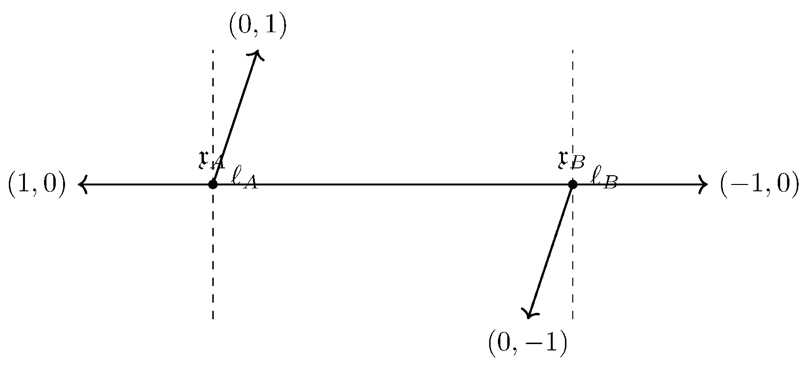
Place two junction points at
for some . At we take charges
so that and are external legs and is an internal leg pointing toward . At we choose
where and are external legs and is the internal leg arriving from . Each junction satisfies charge conservation:
The two internal legs are simply the same physical segment with opposite orientations. For a constant axio–dilaton one can again arrange all legs at appropriate angles so that tension vectors close at each junction. A schematic planar picture is shown in Figure 2.
- Local neighborhoods and FFs on the web.
We choose small neighborhoods
around points on the three legs meeting at , and similarly
around points on the three legs at . The internal segment between and is covered by the pair and , which overlap in a small open interval around the midpoint of the internal edge. We set
Over each and we place the same S-dual FFs
with
and we associate primary fields to the external legs:
The internal segment is then naturally associated to the first mixed level in the FF grading (e.g. the mode in the example), and its excitations are described by auxiliary or mixed fields in the combined -grading.
- Gluing of modal data along the internal edge.
Let and be the associated fuzzy propositions, as before. At each junction point and we have normalized truth-values
for instance using the dyadic values from the numerically explicit FF example:
and so on for the higher descendants.
To describe propagation along the internal edge, we introduce an attenuation factor
which captures the net effect of transport from to through the internal -source and the modal lightcone. At the level of fuzzy truth-values, this is encoded by a simple gluing rule:
for any proposition that is transported along the internal leg. More refined models can replace (46) by an integral kernel or a spectral projection built from the -source geometry; for this minimal web it suffices to keep a single scalar parameter.
As a concrete example, take and consider the composite proposition
which states that “ is active at the left junction and is active at the right junction.” Using the product t-norm for ∧, the glued truth-value is
Thus the joint activation across the two-junction web sits two dyadic steps further from the realized apex than alone, and one step further than the single-junction composite discussed earlier. In the modal lightcone picture, this corresponds to moving one layer outward along the dashed, “merely possible” region.
- Kripke frame viewpoint.
Formally, we can regard the minimal web as a Kripke frame built from three types of worlds:
- worlds localized near ,
- worlds localized near ,
- worlds along the internal segment.
The accessibility relation R contains:
reflecting causal/modal access along the internal edge. The valuation V of propositions is specified at and by the numbers and , and extended to via the gluing rule (46). The computation (47) is then simply the evaluation of a conjunction over the composite path
in the frame.
In this way, even this minimal web realizes the full stack of structures introduced in the paper: a Minkowski lightcone apex at each junction, internal -sources controlling attenuation and mode selection on the internal edge, S-dual FFs attached to each leg, and a Kripke/modal semantics that computes concrete, normalized truth-values for composite propositions across the web.
6. Discussion and Outlook
The inception of this paper began by considering Minkowski lightcones not merely as geometric objects, but instead decorated structures endowed with modal and fuzzy information. This ties into a general desire to fill the lacuna of non-classical logics in physics. While heterodox, the framework here is deliberately modest; propositions are mere proxies for field content of fields . We implemented a rather standard M-theoretic -compactification, in which the relativistic information is contained in a thickened apex of a global lightcone spanning the whole of spacetime.
This gave rise to “eternal" photons , which are unphysical modes that required us to truncate the modal histories by fixing finite sub-lightcones containing the apex ℓ. The kinematic aspects of this neighborhood are regarded as ℓ-packets, which are a souped up version of the classical notion of wave-packets, that factor through the present moment, or in other words, the necessary frame □.
We also gave □ a dual role by implementing a map in Equation (1), which we localized in Equation (8), all while connecting to our previous work ([7] was implemented in (11) and (12), and [6] was discussed throughout), cementing the narrative within a larger research program. The implementation of the decorated loop-space (DLS) paradigm forced us to consider vibrational modes of closed strings as probabilistic phenomena, which then generalized to the open case via a similar procedure.
On top of this modal, we introduced interstices
as higher-dimensional avatars of Chan–Paton defects on open strings, now sitting at junctions in a compactified background. Each interstice carries an internal -source fiber and supports S-dual field-families (FFs) and , together with a grading that separates primary, descendant, and auxiliary fields. We showed how a House–Lukas–Micu type superpotential can be reinterpreted as a modal flux superpotential, with its real part feeding into the exponents in , and how nilpotent overshoots beyond naturally realize the “eternal photon” as a degenerate, unphysical mode in the -source directions.
The FF formalism allowed us to attach concrete S-dual data to junctions and webs. We constructed both a numerically explicit toy model of FF activation on a three-leg junction and a minimal web with two junctions connected by an internal segment. In each case, we made the -valuations completely explicit, used a product t-norm to evaluate composite propositions such as , and tracked the attenuation of truth-values along the internal edge via a simple gluing rule. Viewed as a Kripke frame, the web becomes a small network of worlds connected by an accessibility relation that respects the geometry: modal transitions along the web are the logical shadow of charge-conserving, tension-balanced configurations in Type IIB.
Several limitations of the present treatment are worth emphasizing. First, we worked with simple, static junctions and webs in a fixed-time slice of , with constant axio–dilaton and a highly idealized compact factor. The internal -source geometry entered only through its torsion scalar and a schematic differential D, rather than via explicit solutions of the eleven-dimensional equations of motion. Second, our choice of t-norm and the scalar attenuation parameter along the internal edge were made for concreteness, not uniqueness: other fuzzy-logical choices and more structured transport operators (e.g. spectral projections built from the Laplacian) may be more appropriate in specific physical applications. Finally, we restricted attention to finite FFs and simple coprime gradings; richer charge lattices and higher junction multiplicities will require a more elaborate combinatorial organization.
Despite these simplifications, the formalism suggests several concrete directions for further work:
- Larger webs and networks. Extend the Kripke/FF construction to general webs and five-brane webs, analyzing how -valuations glue along networks with nontrivial cycles and how nilpotent modes behave under web deformations.
- Dynamical and supergravity embeddings. Embed the modal lightcone and -source picture into explicit eleven-dimensional backgrounds, for example by solving the weak Killing spinor equations with flux and comparing the resulting spectrum to the FF grading and the modal flux superpotential.
- Defects and modal healing. Make precise the relationship between interstices and Chan–Paton defects, importing the entropy modal index and MacNeille-type “modal healing” procedures to repair inconsistent -valuations across webs with defects.
- Categorical and operadic refinements. Recast FFs and interstices in terms of higher categories or operads of junctions, so that the modal lightcone and -sources become part of a functorial assignment of logical data to extended configurations, in line with TQFT and decorated loop-space approaches.
Taken together, these directions point toward a broader program in which spacetime lightcones, internal flux geometries, and logical modalities are treated on the same footing.
Appendix A. The Bicategory of Strings
In this section we formalize the basic categorical setting in which our string-theoretic constructions take place. The guiding principle is that the data carried by an open string decomposes into two logically distinct components:
- a geometric component, represented by a Moore path in a configuration space X, and
- an internal component, represented by Chan–Paton labels, F-terms, and other worldsheet operators.
These two components naturally form enriched categories in their own right, and the interaction between them is governed by a heteromorphism bifunctor that factors through a product enrichment category. This leads to a clean definition of the string bicategory, denoted .
The Moore Path Category
Let X be a fixed topological space. The Moore path category is the -enriched category defined as follows.
Definition 3.
The objects of are points of X. For , the hom-object is the topological space
equipped with the compact–open topology. Composition is given by Moore concatenation:
with
Identities are the constant paths of length 0. This makes a strict -enriched category.
Moore paths give strict associativity without reparametrization, which is the correct behavior for concatenation of physical string segments.
The Internal Term Category
Internal data carried by a string endpoint—including Chan–Paton factors, representations, and worldsheet operators such as F-terms—is encoded by a separate enriched category.
Definition 4.
Let denote a convenient category of “matrix objects”: for example, finite-dimensional vector spaces with distinguished bases and linear maps represented by matrices. The term category is a -enriched category whose objects are internal sectors (Chan–Paton labels, flavor representations, etc.). For internal sectors , the hom-object
consists of the matrix data corresponding to allowed worldsheet terms from A to B. These morphisms include, in particular, F-terms and other operator insertions.
The enrichment in allows us to keep track of gradings, superpotentials, and other algebraic structures that arise naturally in supersymmetric string theories.
A Product Enrichment Category
To combine geometric and internal information without collapsing either structure, we work in the product enrichment category
An object of is a pair with and , and the monoidal structure is defined componentwise. Both and embed canonically into -enrichment:
Heteromorphisms Between Path and Term
Geometric and internal data interact through a set-valued heteromorphism functor. Formally:
Definition 5.
A heteromorphism from a path object to an internal object is an element of a set
where is a bifunctor. Precomposition in and postcomposition in define the bifunctoriality structure.
Crucially, these heteromorphisms arise from enriched data:
Proposition 1.
There exists a -valued bifunctor
such that
where is the functor sending to the underlying set .
Thus every heteromorphism “comes from” combined topological and matrix structure; the set-theoretic description used in the bicategory is merely its shadow.
The String Bicategory
We now assemble the above ingredients into a bicategory with two distinguished regions: a geometric region and an internal region.
Definition 6.
The string bicategory is the bicategory obtained as the collage of the heteromorphism bifunctor . Its 0-cells are two enriched categories, and . Its 1-cells consist of:
- morphisms in (geometric evolution of endpoints),
- morphisms in (internal evolution, including F-terms),
- heteromorphisms from geometric to internal sectors.
The 2-cells are generated by the enriched structures in , , and their product .
Appendix B. Kripke Frames and Accessibility
For the reader’s convenience, we briefly recall the standard Kripke semantics for propositional modal logic and explain how it relates to the accessibility relation implicit in equation (5) and the modal lightcone in Figure 1.
Definition 7
(Kripke frame). A Kripke frame is a pair consisting of a nonempty set W of worlds and a binary relation , called the accessibility relation.
Definition 8
(Kripke model). A Kripke model on a frame is a triple where is a valuation assigning to each propositional variable p the set of worlds in which p is true.
Given a model , the satisfaction relation for a world and a formula is defined inductively in the usual way for Boolean connectives. The modal operators □ and ♢ are interpreted via the accessibility relation:
Thus □ expresses truth at all R-accessible worlds, while ♢ expresses truth at some R-accessible world.
Relating Kripke Frames to the Modal Lightcone
In the setting of Section 3.1, let denote the space of field configurations along the string , and let be the time-evolution maps introduced in (3)–(4). Fix a reference time and consider the set
of configurations obtained by iterating the dynamics forward and backward (to the extent that this is defined). We define an accessibility relation R on W by declaring that if and only if v is obtained from w by a single time-step of the dynamics:
The pair is then a Kripke frame in the sense of Definition 7. The nodes in Figure 1 can be viewed as a finite subframe generated from a distinguished “present” configuration by iterating R into the past and future. The labels and record, respectively, R-predecessors and R-successors of .
Fix now a point , and consider the local algebra of propositions about the behavior of fields in the neighborhood as in Section 3.1. A valuation
is obtained by declaring, for each proposition , the set to consist of those configurations whose restriction to satisfies . The resulting Kripke model then reproduces the semantics of the local modal operators and defined in (5)–(7): equations (A1) and (A2) specialize to
where the satisfaction relation on the right-hand side is now interpreted in terms of the local behavior of the fields near .
Under this identification, the modal lightcone of Figure 1 is nothing but a finite fragment of a Kripke frame , together with a distinguished world and its R-successors and R-predecessors, decorated by the iterated modalities .
Appendix C. Toy Examples
Modal Expectation Value at a Single Point
In this subsection we spell out a concrete finite-depth toy model of the modal expectation value
from Equation (26). The goal is not realism, but to give a small example in which all of the sums appearing in (22)–(26) become literally finite.
Fix a point and a field configuration . Instead of the full update monoid , we truncate to a finite-depth monoid
where is a fixed cutoff. In this toy model we only allow time steps, and regard deeper futures as irrelevant or suppressed.
For each we define the localized action at time by
which is just the localized action (14) evaluated on the time-evolved configuration . We can package these into a truncated generating functional
where the coefficients play the same role as in (20)–(22), but the sum is now finite.
To interpret this in probabilistic terms, we choose a family of formal weights
satisfying the normalization condition
in . These weights can be viewed as a formal probability distribution on the truncated monoid , assigning to each depth n in the modal lightcone a formal likelihood .
The corresponding truncated modal expectation value of the localized action at is then
If we set for all , then
which is the finite-depth analogue of equation (27). In particular, the toy model shows explicitly how:
- the discrete time-steps index layers of the modal lightcone at ,
- the spatial data enter through the localized actions in (A6), and
One can, of course, choose explicit values for the and to obtain fully concrete examples. For instance, taking and working to leading order in ℏ, one may model
with and classical probabilities satisfying . Then (A10) reduces to the familiar finite weighted average
which can be regarded as the shadow of the more general formal expectation (A10).
A Toy Model of S-Dual Field-Families on a Three-Leg Junction
In this appendix we spell out a concrete toy model of the S-dual field-families (FFs) introduced in the main text. The goal is purely illustrative: we want an example where the grading, the auxiliary fields, and the interstice sector can all be written down explicitly.
We take
so that p and q are relatively coprime, and consider the S-dual FFs
living on the disjoint union
of neighborhoods around three points on the legs of a string junction. As in the main text, each field has an associated fuzzy proposition:
encoding “ is active” and “ is active” as Heyting–Kripke propositions.
We use the number-theoretic grading
to organize all fields, with
The first few values are:
Here give descendants of , while give descendants of . The integers with (e.g. ) label auxiliary fields that lie “between” the pure - and pure -descendants in the grading. The value is a least common multiple and corresponds to a mixed S-dual mode; in a more refined model, one can distinguish this from the purely auxiliary levels by tracking the pair of charges in the -lattice.
On the geometric side, we fix an interstice
and define, for each pair , the interstice sector
as in (41). In this toy model we focus on the simplest nontrivial choice
so that the fundamental interstice sector is
and S-duality acts by the standard action on the column vector .
To connect this to the fuzzy semantics, we assign to each proposition and a normalized truth-value
via
for some fixed base . For instance, one may take
so that and are “closest” to the realized history at the apex in the sense of Figure 1, while higher-index fields are increasingly suppressed. The auxiliary levels can be assigned truth-values by any monotone rule compatible with (A12); for example, one may set
with chosen so that always lies between the neighboring descendants in the grading.
Finally, the nilpotent “eternal photon” deformation appears here when we attempt to push a given beyond 1 by adjoining an infinitesimal:
In the extended truth-value ring this defines a degenerate mode that has no effect on the underlying support of the interstice sector
but records an infinitesimal, unphysical perturbation of the -source at the junction. Projecting back to annihilates the -part and restores the physical truth-value. Thus even in this toy model we see explicitly how the grading of FFs, the S-dual structure, and the nilpotent -modes can coexist within a single, finite combinatorial pattern.
References
- O. Aharony, A. Hanany, and B. Kol, “Webs of (p,q) five-branes, five-dimensional field theories and grid diagrams,” J. High Energy Phys. 01 (1998), 002. arXiv:hep-th/9710116. [CrossRef]
- J. C. Baez and M. Stay, “Physics, Topology, Logic and Computation: A Rosetta Stone,” in New Structures for Physics, Lecture Notes in Physics, vol. 813, Springer, 2010, pp. 95–172. Available at arXiv:0903.0340. [CrossRef]
- G. Birkhoff and J. von Neumann, “The Logic of Quantum Mechanics," in Annals of Mathematics, Vol. 37, No. 4, October, 1936. [CrossRef]
- P. Blackburn, M. de Rijke, and Y. Venema, Modal Logic, Cambridge Tracts in Theoretical Computer Science, vol. 53, Cambridge University Press, 2001.
- J. V. Corbett A Topos Theory Foundation for Quantum Mechanics (2012) available: arXiv:1210.0612v1 [quant-ph]. [CrossRef]
- R. J. Buchanan and P. Emmerson, “Phenomenology of Chan–Paton Defects on Open Strings," Authorea preprint. (2025). [CrossRef]
- R. J. Buchanan, “Decorated Loop-Spaces I: Foundations and Applications,” Authorea preprint. (2025). [CrossRef]
- P. Galison, “Minkowski’s Space-Time: From Visual Thinking to the Absolute World,” Historical Studies in the Physical Sciences 10 (1979), 85–121. [CrossRef]
- T. House and A. Micu, “M-theory compactifications on manifolds with G2 structure,” Classical and Quantum Gravity 22 (2005) no. 9, 1709–1738, hep-th/0412006. [CrossRef]
- T. House and A. Lukas, “G2 domain walls in M-theory,” Physical Review D 71 (2005) 046006, hep-th/0409114. [CrossRef]
- T. House, Aspects of Flux Compactification, DPhil thesis, University of Sussex, 2005.
- S. A. Kripke, “Semantical Considerations on Modal Logic,” Acta Philosophica Fennica 16 (1963), 83–94.
- B. Kol, “(P,Q) Webs in String Theory,” Ph.D. thesis, Stanford University, 1998. Available via ProQuest Dissertations & Theses, docview:304455946.
- M. Markl, “Operads and PROPs,” in Handbook of Algebra, vol. 5, Elsevier/North-Holland, Amsterdam, 2008, pp. 87–140. See also arXiv:math/0601129.
- M. Markl, S. Shnider, and J. Stasheff, Operads in Algebra, Topology and Physics, Mathematical Surveys and Monographs, vol. 96, American Mathematical Society, Providence, RI, 2002.
- H. Minkowski, “Raum und Zeit,” Physikalische Zeitschrift 10 (1909), 104–111. English translation “Space and Time” in The Principle of Relativity, H. A. Lorentz, A. Einstein, H. Minkowski, and H. Weyl, translated by W. Perrett and G. B. Jeffery, Dover, New York, 1952, pp. 73–91.
- J. Polchinski, String Theory, Vol. 2, Cambridge Monographs on Mathematical Physics, Cambridge University Press, 1998.
- P. K. Townsend, “p-Brane Democracy,” in The World in Eleven Dimensions: Supergravity, Supermembranes and M-Theory, ed. M. J. Duff, IOP Publishing, Bristol (1999), pp. 375–389, arXiv:hep-th/9507048.
- J. H. Schwarz, “The Early History of String Theory and Supersymmetry,” in Subnuclear Physics: Past, Present and Future, Pontifical Academy of Sciences, Scripta Varia, vol. 119, Vatican City, 2014, pp. 69–83. Available at sv119-schwarz.pdf.
- M. B. Green, J. H. Schwarz, and E. Witten, Superstring Theory, Vols. 1–2, Cambridge Monographs on Mathematical Physics, Cambridge University Press, 1987.
- E. Witten, “String theory dynamics in various dimensions,” Nucl. Phys. B 443 (1995) 85–126, https://arxiv.org/abs/hep-th/9503124. [CrossRef]
| 1 | See in particular the bimodule formulation of Chan–Paton factors and the role of defects as projectors that partition an open string into and while breaking epistemic harmony; cf. [6]. |
| 2 | For historical overviews, see for example [19] and references therein. Dualities had grown increasingly important during the 1950s, when physicists realized that -decay did not respect parity symmetry; famously, Lee and Yang won the nobel prize for this discovery, while experimentalist Wu did not. |
| 3 | For a classic account of the superstring revolution and anomaly cancellation, see e.g. [20]. |
| 4 | |
| 5 | We flesh out a version in 40 with a bit more detail. |
| 6 | For simplicity we treat the time evolution as generated by a single one-parameter family ; multiple background fields or couplings could be included as additional indices without changing the discussion. |
| 7 | We record the details for the categorically-minded reader in Appendix A. |
| 8 | For a simple implementation of this setup, we defer to the Appendix C. |
| 9 | For brevity, we have re-written as . |
| 10 | |
| 11 | |
| 12 | See, e.g., the Freund–Rubin compactification. References can be found in [11]. |
| 13 | Those familiar with the Newton lore might call these “fluxions.” |
| 14 | This allows us to substitute the units of frequency for the ℓ-packet; contravariance means that by decreasing our -length, we increase . |
Figure 1.
Modal lightcone of string vibrational modes. The central node represents the present string configuration, viewed as a modal singularity of the lightcone. Nodes labeled by positive powers (, ) correspond to higher modal iterates of the string state, while negative powers (, , , ) encode modal predecessors. Dashed arrows indicate kinematically accessible future string states, the solid arrows trace the actually realized history feeding into the present configuration, and the squiggly arrows represent cancelled or unrealized trajectories in the modal dynamics.
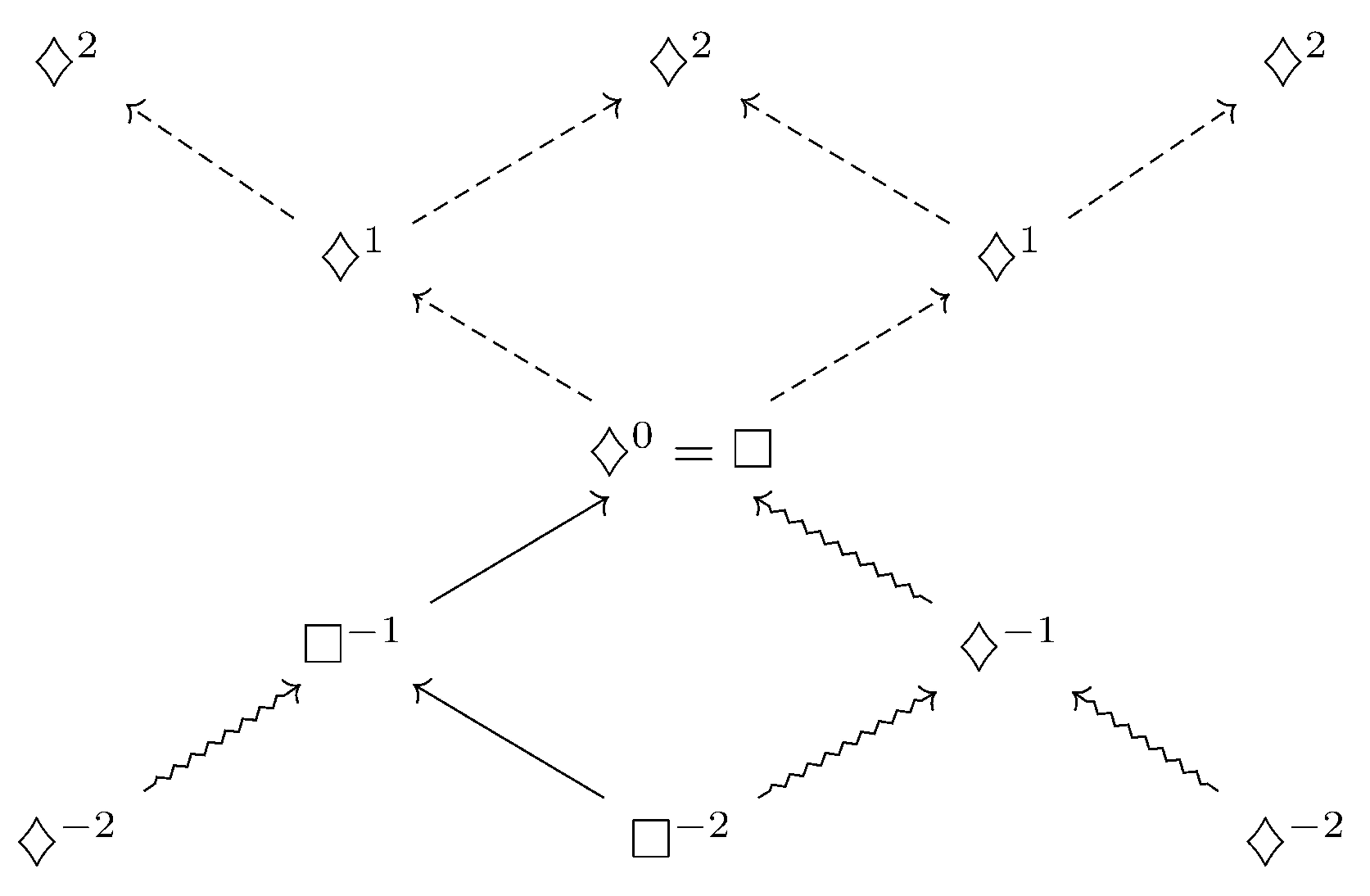
Figure 2.
A minimal web with two three-string junctions at and connected by an internal segment. At , the external legs carry charges and , and the internal leg carries . At , the external legs carry and , and the internal leg carries . Dashed lines indicate the local lightlike directions through the modal apices and .
Disclaimer/Publisher’s Note: The statements, opinions and data contained in all publications are solely those of the individual author(s) and contributor(s) and not of MDPI and/or the editor(s). MDPI and/or the editor(s) disclaim responsibility for any injury to people or property resulting from any ideas, methods, instructions or products referred to in the content. |
© 2025 by the author. Licensee MDPI, Basel, Switzerland. This article is an open access article distributed under the terms and conditions of the Creative Commons Attribution (CC BY) license.
Copyright: This open access article is published under a Creative Commons CC BY 4.0 license, which permit the free download, distribution, and reuse, provided that the author and preprint are cited in any reuse.


