Submitted:
17 December 2025
Posted:
18 December 2025
You are already at the latest version
Abstract
This study examines the time evolution of structural and informational quantifiers in a damped Rabi oscillator, specifically focusing on fidelity, entropy, disequilibrium, and Fisher information. We observe that all four measures exhibit damped oscillatory behavior as the system approaches its steady state. However, the final asymptotic behavior is striking: while fidelity and disequilibrium indicate a residual, non-zero final state, and entropy quantifies the thermodynamic disorder, Fisher information uniquely vanishes. This vanishing implies a complete loss of dynamical information—the ability to infer the system's past evolution from its current state—even in the absence of complete thermodynamic disorder. Our findings introduce a new phenomenon where a system can be "informationally silent," meaning it becomes structurally ordered yet loses all inferential sensitivity to its own history, a detail that traditional entropy measures do not fully capture. This work highlights a critical distinction between thermodynamic disorder (entropy) and inferential sensitivity (Fisher information) in the context of open quantum systems.
Keywords:
fisher information
; rabi oscillator
; decoherence
; information degradation
1. Introduction
The Rabi oscillator [1,2] illustrates the fundamental principle of quantum coherence, which is the ability of a quantum system to exist in a superposition of states and to evolve smoothly and periodically under the influence of an external field. It shows how a two-level quantum system can periodically transition between its ground and excited states due to coherent interaction with an oscillating field, unlike classical systems which would have discrete absorption and emission events. Indeed, Rabi oscillations are a direct manifestation of quantum coherence. The system’s state is not simply “here" or “there" but is a coherent superposition of both the ground and excited states. This allows for a smooth, cyclical exchange of energy, which is different from a purely classical process. As the system interacts with the driving field, its probability of being in the ground state and the excited state oscillates periodically, a phenomenon known as “Rabi flopping". The oscillations arise from the combined process of stimulated absorption and emission. The energy is transferred from the field to the atom (absorption) and then back to the field (stimulated emission) in a repeating cycle. While Rabi-like oscillations can be observed in classical systems (like two coupled pendulums), the Rabi oscillator in a quantum system is driven by a more fundamental quantum mechanical principle: the coherent evolution of the system’s wave function, which leads to predictable and periodic transitions between quantum states Accordingly, Rabi oscillation is important because it demonstrates a fundamental principle of quantum mechanics and is essential for controlling and manipulating quantum systems. Its importance spans a wide range of applications, including the development of quantum computing, quantum computing logic gates and quantum information processing, and technological advancements like nuclear magnetic resonance (NMR) spectroscopy and imaging. By precisely controlling the oscillation frequency and duration of an external field, it is possible to transfer a quantum system between states, a process that is crucial for achieving quantum operations. Some applications of Rabi oscillation are:
- Quantum computing: The phenomenon provides a physical mechanism for performing spin flips in a two-level quantum system, which is a qubit. By applying a pulse of specific duration and intensity, a qubit can be manipulated to be in a superposition of states, a key requirement for quantum computations.
- Quantum optics: Rabi oscillation is used to describe how a two-level atom, like one in a ground and excited state, interacts with an electromagnetic field. This allows for precise control over light-matter interactions.
- Precision measurements: Rabi oscillations are fundamental to techniques such as stimulated Raman adiabatic passage (STIRAP), which is used for high-precision control of quantum systems.
- Spectroscopy: The phenomenon is a cornerstone of techniques like nuclear magnetic resonance (NMR) and electron spin resonance (ESR). By observing the Rabi oscillations, scientists can extract information about the properties of a quantum system.
Let us insist: our system is a cornerstone of quantum mechanics because it shows how to coherently transfer the population of a quantum system from one state to another by applying an oscillatory driving field and because Rabi oscillation provides a direct method for controlling the state of a quantum system, which is the basis for building quantum technologies. The decay of Rabi oscillations (known as transient nutations) gives direct information about the coherence time of the system, which is critical for understanding and overcoming decoherence in quantum computation. The phenomenon provides a physical mechanism for performing spin flips in a two-level quantum system, which is a qubit. By applying a pulse of specific duration and intensity, a qubit can be manipulated to be in a superposition of states, a key requirement for quantum computations. We suggest consulting Refs. [3,4,5,6,7,8,9,10,11,12,13,14,15,16,17,18,19,20,21,22,23,24].
1.1. Information Quantifier Used Here
Fisher Information in the Damped Rabi Oscillator is crucial for understanding how a quantum system loses information due to dissipation and decoherence. Fidelity measures the overlap between the initial and time-evolved states, showing how the system’s quantum information is lost. Entropy provides a measure of the system’s uncertainty or disorder, and Disequilibrium quantifies the deviation from a steady state. Fisher Information is particularly important because it quantifies the precision of parameter estimation and can be used to detect quantum phenomena like synchronization, even when other measures fail [3,4,5,6,7,8,9,10,11,12,13,14,15,16,17,18,19,20,21,22,23,24]. Let us now delve on the importance of each of these quantifiers:
- Fidelity: it a) quantifies the loss of quantum coherence in the system over time, b) helps determine the overall purity and structural integrity of the quantum state. c) A decline in fidelity indicates that the system is losing the ability to preserve quantum states accurately, which is a key indicator of how well information is being transmitted or stored.
- Entropy: it a) measures the degree of “disorder" or the spread of the system’s probability distribution. b) In the context of the Damped Rabi Oscillator, it shows how information spreads out as the system loses energy and coherence. c) By tracking entropy, researchers can identify how the system’s uncertainty increases over time due to damping and decoherence.
- Disequilibrium: it a) quantifies the system’s deviation from its final equilibrium state. b) In the Damped Rabi Oscillator, it shows how far the system is from reaching a steady state and helps describe the dynamics leading to it. c) It is a useful measure for understanding how a system is evolving and how it approaches a stable, thermal state in the presence of dissipation.
- Fisher Information: it a) provides a measure of the precision with which a parameter can be estimated from the system’s state. b) It is a sensitive probe of quantum features, unlike entropy which can be insensitive to certain types of information loss. c) In the Damped Rabi Oscillator, Fisher information can reveal phenomena like the “trapping" of information, where the system becomes “informationally silent" but still retains some structural order. d) It is a powerful tool for metrology and can be used to detect quantum synchronization, even when other measures fail.
The organization of the paper is as follows. Section 2 provides a brief contextual introduction to the Rabi model and to the dissipative mechanisms relevant for the driven two-level system. Section 3 introduces the Lindblad master equation and presents the derivation of the Bloch equations that describe the damped dynamics. Section 4 develops the Fisher-information formalism for the two-level dynamics and provides the unified expression valid in all dissipative regimes. Section 5 defines the Shannon entropy for the two-level system and gives the explicit time-dependent expression used in our analysis. Section 6 introduces disequilibrium and the LMC statistical complexity and applies them to the Rabi populations. Section 7 is devoted to the analysis of the fidelity, where we discuss its behavior under dissipation and its usefulness as a measure of coherence loss in the driven system. In Section 8, we define the additional information-based quantifiers used in this work –entropy, disequilibrium, and Fisher information– and comment on the specific dynamical features each one captures. Finally, Section 9 summarizes the main findings and outlines possible extensions of this framework to other driven open quantum systems.
We remark finally that relevant complementary studies include treatments of quantum Fisher information under dissipation [20], geometric formulations of decoherence and information contraction [21,22], and the thermodynamic length in quantum systems [23,24], which provide a natural conceptual framework for the informational degradation to be observed here.
2. Historical Context of the Rabi Model
The Rabi model [1], introduced in 1937 by Isidor Isaac Rabi [1], describes the simplest quantum interaction between a two-level system (spin- particle) and a classical oscillating field. Originally developed to explain the magnetic resonance of atomic nuclei in a rotating magnetic field, the Rabi model laid the groundwork for nuclear magnetic resonance (NMR), electron spin resonance (ESR), and numerous spectroscopic techniques.
The key insight of Rabi’s work was the prediction of coherent oscillations between the two atomic states when subjected to a resonant field–what are now called Rabi oscillations. These oscillations reflect the time-dependent probability of population inversion in a driven two-level system and remain a cornerstone of coherent control in modern quantum technologies.
While the original Rabi model involves a classical driving field, it serves as the conceptual forerunner of fully quantum models such as the Jaynes-Cummings model, where the field itself is quantized. Nonetheless, the classical Rabi model retains fundamental importance due to its exact solvability and analytical accessibility under both resonant and detuned driving conditions.
With the advent of quantum computing and coherent control platforms (e.g., trapped ions, superconducting qubits, and NV centers in diamond), the Rabi model has gained renewed relevance. It underpins control protocols, gate dynamics, and the study of decoherence in driven quantum systems. Moreover, it has been generalized to include counter-rotating terms (yielding the quantum Rabi model), dissipative environments, and even multi-photon interactions.
In this work, we revisit the Rabi model from a quantum information-theoretic perspective. By coupling the two-level system to a classical drive and incorporating Lindblad-type dissipation, we expose a novel mechanism for informational degradation –the vanishing of Fisher information– even as the system retains low entropy and structural coherence. This highlights the Rabi model’s continuing power as a theoretical laboratory for probing the boundaries of coherence, inference, and irreversibility in open quantum systems.
2.1. Exact theory of damped Rabi oscillations
One must have in mind, before proceeding, the importance and interesting findings on Ref. [1], that deal with a driven two-level system subject to dissipation exhibits Rabi oscillations whose amplitude decays due to population loss and dephasing. While the standard phenomenological model employs a single exponential envelope, an exact analysis shows that open-system Rabi dynamics generically contain three distinct decay channels. This structure was derived in full generality by Kosugi et al. [2], who extended Torrey’s Laplace-transform method to include both internal relaxation and external loss mechanisms.
The starting point is the driven Hamiltonian matrix
together with four dissipative rates: decay from the excited and ground states ( and ), internal relaxation (), and pure dephasing (). Introducing the usual Bloch variables for coherence and population inversion, and for total population, the master equation reduces to a linear system with . Unlike the closed Bloch equations, is no longer conserved because of population leakage.
The exact solution for each component has the universal form
revealing two purely decaying exponentials (, ) and one damped oscillation with frequency s and decay constant c. For experimentally relevant near-resonant driving (), the excited-state population is well approximated by
where and with . This expression explains several features observed experimentally in driven Josephson phase qubits—including asymmetric upper and lower envelopes, multiple decay rates, and non-zero initial excited-state population—that are not captured by the usual single-exponential model.
An important practical outcome of Ref. [2] is a method for extracting all relaxation rates from the measured envelopes of the damped oscillation. By forming the combinations and , one obtains two single-exponential curves with decay constants a and c. Together with the free-evolution decay rates in the absence of driving, these yield closed-form expressions for , , , and , allowing a complete reconstruction of decoherence channels in the two-level system.
3. Lindblad Formalism for the Damped Rabi Oscillator
Our references in this Section are [14,15] To incorporate decoherence, we adopt the Lindblad master equation for Markovian open quantum systems [14,15]. The time evolution of the density matrix is
where is the spontaneous emission rate, , and . The coherent part is governed by the driven two-level Hamiltonian
where and denote the Pauli matrices. Here, is the (bare) Rabi frequency, proportional to the strength of the coherent driving field, while is the detuning between the laser frequency and the internal transition frequency . The term proportional to induces coherent population oscillations between the ground and excited states, while the term proportional to reflects the energy splitting in the rotating frame.
The origin of each contribution is as follows [14,15]: the terms proportional to and arise from the coherent commutator and generate Rabi oscillations, whereas the terms proportional to originate from the Lindblad dissipator. The latter cause irreversible decay of the excited-state population () and exponential damping of coherences ( and ), driving the system toward the ground state. Units with are assumed throughout.
3.1. Bloch Equations, Analytic Solution and Dissipative Regimes
3.1.1. Bloch-Equation Representation
Starting from the Lindblad equation (4) with Hamiltonian (5), it is convenient to rewrite the dynamics in terms of the Bloch variables [14,15]
One obtains the dissipative Bloch equations
3.1.2. Closed-form solution for (initial ground state)
We consider the initial condition , i.e., .
In the underdamped regime [14,15] , the solution for the density-matrix elements in the basis reads
with . These expressions are algebraically equivalent to the solution obtained by solving the linear system (7) and reconstructing .
3.2. Unified Expression for All Dissipative Regimes
For later use in Fisher information, Shannon entropy and LMC complexity, we adopt a single compact expression valid for underdamped, critically damped, and overdamped regimes [14,15]. Introduce unified trigonometric/hyperbolic functions
Then the excited-state population takes the compact form
3.3. Coherent and Dissipative Limits
Before analyzing the behavior of information-theoretic quantifiers, it is useful to summarize the main limits and dynamical regimes implied by the Lindblad solution [14,15]. Setting recovers the coherent Rabi evolution with generalized Rabi frequency ,
which will serve as a reference for the dissipative case. The complete density-matrix solution also satisfies the expected conditions , , and , and in the long-time limit it relaxes to for any .
Dissipation modifies the coherent dynamics through the parameter
which determines the qualitative behavior of the system:
- Resonant case (): the effective frequency reduces to . Oscillations persist only in the underdamped regime ; otherwise the dynamics become non-oscillatory.
- Underdamped (): damped oscillations at frequency , modulated by , and
- Critical (): oscillatory and relaxational timescales coincide, yielding the slowest non-oscillatory response.
- Overdamped (): no oscillations occur; the dynamics become purely relaxational with rates
4. Fisher Information: Discrete Definition and Rabi Applications
4.1. Discrete Fisher Information
We consider a discrete distribution depending on a parameter , with . The Fisher information is defined as [3,16]
For a two-level system with and , choosing yields
Using the unified expression (14) one finds
and therefore the Fisher information takes the compact unified form:
This expression is valid in all dissipative regimes.
4.2. Coherent Limits
For and arbitrary detuning, Eq. (18) reproduces
For the resonant undamped case (), one recovers the constant result .
5. Shannon Entropy and Rabi Applications
5.1. Definition
Shannon entropy was formally introduced by Shannon in 1948 with the purpose of mathematically quantify the statistical nature of lost information in communication systems and to define a measure of uncertainty [17].
For a discrete probability distribution with and the Shannon entropy is defined as
This time-dependent entropy provides a quantitative measure of the information content associated with the population dynamics. This quantity measures the statistical uncertainty (or information content) associated with the distribution. It satisfies with the lower bound reached for a fully certain distribution (one outcome with probability 1), and the upper bound reached for the uniform distribution .
5.2. Shannon Entropy for a Two-Level System
For a driven two-level system the relevant probability distribution is where is the excited-state population obtained from the Lindblad dynamics. In this case the Shannon entropy reduces to the binary form
This expression will be used below to construct the disequilibrium and the LMC complexity.
Inserting the general form of gives
which is an explicit closed expression valid in all regimes.
6. LMC Complexity
6.1. Definition
The LMC (López-Ruiz, Mancini and Calbet) statistical complexity is defined as [18]
where is the normalized Shannon entropy and D the disequilibrium. For a discrete distribution of N states the normalized entropy is
and the disequilibrium, that quantifies the departure of the system from the uniform distribution, is defined as
6.2. Rabi Applications
For the two-level system (), the disequilibrium, defined as the deviation from maximal mixedness, becomes
The disequilibrium vanishes at the fully mixed state , and increases as the distribution becomes more peaked.
In this case, the normalized Shannon entropy is
with given by Eq. (20). Therefore, the LMC complexity is given by
This quantity is minimal both for perfectly ordered states () and for the maximally mixed state (), reaching its maximum at intermediate levels of disorder and disequilibrium.
7. Fidelity in Dissipative Dynamics
In the presence of dissipation, the time evolution of the two-level system is no longer unitary and the state of the system is described by a density matrix satisfying the Lindblad master equation (4). Since the state ceases to be pure for , the usual expression for pure states is no longer applicable. Instead, we employ the Uhlmann fidelity [19], which provides a consistent extension of state overlap to arbitrary mixed states.
7.0.0.1. Uhlmann fidelity.
For two density matrices and , the fidelity is defined as [19]
This expression reduces to the pure-state overlap whenever one (or both) of the states is pure.
7.0.0.2. Fidelity with respect to a reference pure state.
When the target state is pure, , Eq. (26) simplifies to
which is often the most relevant quantity in dissipative quantum dynamics. For instance, choosing yields
so that the fidelity coincides with the excited-state population.
7.0.0.3. Fidelity between dissipative and coherent evolutions.
A useful quantifier of the effect of dissipation is the fidelity between the state evolving under Lindblad dynamics, , and the state that would result from coherent evolution in the absence of decay, . Using Eq. (27), this fidelity is
This measure quantifies the loss of coherence and population induced by spontaneous emission. In particular, as , while for it decays in time as the system relaxes toward the ground state.
The Uhlmann fidelity provides a natural extension of overlap-based quantifiers to dissipative systems and is therefore consistent with the use of the Shannon entropy, disequilibrium and statistical complexity introduced in the following sections. In the present context, the fidelity can be evaluated analytically once the matrix elements of are known from the Bloch-equation solution.
7.1. Fidelity for the Dissipative Rabi Oscillator
To quantify how much the system remains in its initial state under Lindblad dissipation, we consider the fidelity with respect to the initial pure state. Since the system starts in the ground state , the fidelity at time t reduces to
where is the excited-state population. This expression holds for any Markovian decay model where population leaks from to , and it automatically satisfies the physical requirement .
7.2. Closed Expression for the Fidelity
The Lindblad master equation with spontaneous emission rate and Rabi Hamiltonian (5) yields, in the underdamped regime, the well-known analytical solution for the excited-state population given by Eq. (11).
We have the following consistency checks:
The fidelity therefore provides a concise and physically transparent measure of the dissipative evolution, fully determined by the same parameters that govern the Fisher information and Shannon entropy analyzed in previous sections.
8. Quantifiers Interpretation
Figure 1 illustrates the dynamical behavior of the information quantifiers of Shannon entropy , disequilibrium , complexity , fidelity , and Fisher information in the strongly underdamped regime, obtained for , , and a small dissipation rate . In this parameter range the generalized Rabi frequency is dominated by the detuning, , and satisfies , so the system remains close to the coherent limit. Accordingly, all quantities exhibit long-lived oscillations with only a slow exponential decay in amplitude. The coherence displays large-amplitude revivals that follow the unitary oscillation frequency, while the Shannon entropy and the disequilibrium oscillate with comparatively small amplitude, reflecting the fact that the state remains nearly pure during the evolution. The LMC statistical complexity reproduces the same oscillatory pattern, showing intermittent peaks that progressively decrease in magnitude as dissipation accumulates. In contrast to the overdamped regime, the fidelity stays close to unity throughout the dynamics, with only small modulations, indicating that the system does not significantly depart from its initial state. Overall, the figure captures the characteristic signature of the weak-damping regime: persistent Rabi oscillations that imprint their structure simultaneously on entropy, disequilibrium, complexity, coherence, and fidelity.
All five quantifiers display damped oscillations due to coherent Rabi dynamics suppressed by spontaneous emission. The vanishing of Fisher information indicates that, although the system remains structurally ordered, it becomes dynamically silent. That is, infinitesimal changes in time produce negligible statistical differences–an effect we term informational degradation without entropy increase. Our graph illustrates how decoherence, induced by , affects the Rabi-coherent dynamics: the system evolves towards a mixed state. Fisher informational dynamics degrades and one observes the transition from a coherent quantum regime to a more “classical” and stationary one. Such a transition can be said to be the “heart” of the decoherence phenomenon.
Figure 2 illustrates the dynamical behavior of the same quantifiers as in Fig. Figure 1 in the overdamped regime, using the parameters , , and . Since the dissipation rate greatly exceeds the coherent Rabi drive (), the dynamics are fully non-oscillatory. All quantities relax monotonically toward their stationary values as the system is rapidly driven into the ground state by spontaneous emission. The coherence-based quantifier decays on the fastest timescale, reflecting the strong suppression of off-diagonal density matrix elements by the Lindblad damping. The entropy-like measures and display smooth transient behavior without oscillations, reaching steady values once the system approaches its asymptotic state. In contrast, the complexity measure exhibits only a small and short-lived maximum, characteristic of transient mixedness, before vanishing at long times as the system becomes effectively pure. Finally, the fidelity monotonically approaches unity, consistent with irreversible relaxation toward the ground state. Overall, the figure captures the defining features of the overdamped regime, where coherent Rabi oscillations are fully suppressed by strong dissipation.
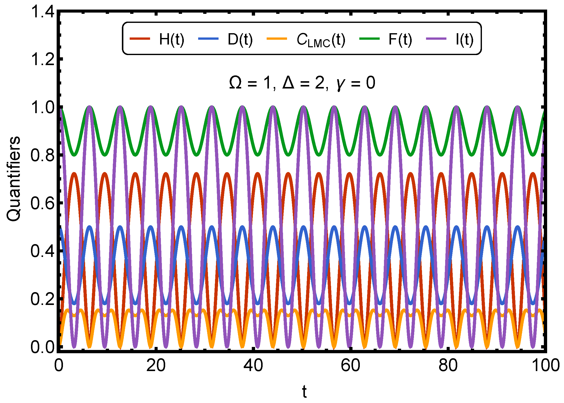
Figure 3 displays the time evolution of the informational quantifiers , , , , and for the resonant Rabi regime, using the parameters , , and . In the absence of dissipation all quantifiers exhibit strictly periodic oscillations governed by the Rabi frequency. Despite sharing the same underlying period, each measure displays a distinct amplitude and dynamical pattern: oscillates around a value close to unity, reflecting the preservation of quantum coherence; fluctuates around a mid-range value with reduced amplitude; and remains confined to very small values, capturing the weak interplay between disorder and structure in this regime. The quantifiers and show faster and higher-contrast oscillations, originating from their nonlinear dependence on the state populations. Altogether, the figure highlights how different informational measures encode complementary aspects of the same coherent two-level dynamics.
9. Conclusions
We have analyzed the time evolution of a set of information–theoretic quantifiers for a dissipative quantum Rabi oscillator governed by a Lindblad master equation. Our results provide a coherent dynamical picture of how coherence, uncertainty, and statistical distinguishability degrade under amplitude damping. By combining entropy-based and Fisher-information-based measures, we were able to track the progressive loss of structure in the system’s quantum state in a quantitatively transparent way.
A central result of this work is the identification of a tight connection between dynamical decoherence and the geometric contraction of the space of quantum states. The decay of the quantum Fisher information, together with the monotonic behavior of entropy and purity, reveals that the dissipative dynamics drives the system along trajectories of decreasing statistical distinguishability, effectively flattening the information-geometric landscape. This establishes a clear dynamical interpretation of decoherence as a loss of statistical resolution rather than merely as a loss of coherence.
Our study shows that information quantifiers provide complementary and physically meaningful diagnostics of open quantum dynamics. Unlike observables tied to specific quadratures or populations, quantities such as Fisher information, purity, and entropy capture universal aspects of quantum state degradation that are independent of basis. This makes them particularly suitable for characterizing decoherence in a model-independent manner.
In the underdamped case, the quantifiers exhibit oscillatory patterns whose amplitudes gradually decrease due to dissipation. While , , and display damped oscillations, the fidelity approaches a stable value and the Fisher information shows a progressive reduction, reflecting a diminishing sensitivity to time-dependent variations in the state. The overall picture indicates that coherence and parameter sensitivity decay at different rates.
In the overdamped regime, the oscillatory structure disappears, and all quantifiers evolve monotonically or with very limited curvature. The figures show that and decay faster than the entropic quantities, indicating that the loss of distinguishability and of parameter sensitivity can precede the full suppression of population imbalance or entropy changes.
At the critical point, where oscillations persist but without decay, the quantifiers remain bounded and display sustained periodic behavior. The results show that , , and oscillate in a stable pattern, while and follow periodic trajectories with different amplitudes and phases. This regime highlights that, even in the absence of damping, the informational indicators do not necessarily evolve in a coherent or synchronized manner.
Taken together, the three regimes illustrate that informational measures respond differently to dissipation and detuning. Entropy and related quantities capture global aspects of population distribution, whereas fidelity and Fisher information are more sensitive to coherence and parameter distinguishability. The combined analysis suggests that a multi-quantifier approach is useful for characterizing the dynamical behavior of driven two-level systems, particularly when one seeks to compare coherence, structure, and sensitivity to external parameters.
Beyond the Rabi oscillator, the framework developed here can be naturally extended to a wide class of open quantum systems, including driven two-level models, harmonic networks, and cavity–QED platforms. The interplay between dissipation and information geometry uncovered in this work suggests that information-based diagnostics can serve as sensitive probes of environmental coupling and may be exploited in the design of robust quantum technologies where control of decoherence is crucial.
Acknowledgments
Research was partially supported by ANID/FONDECYT, grant 1251928.
References
- Rabi, I.I. Space Quantization in a Gyrating Magnetic Field. Phys. Rev. 1937, 51, 652. [Google Scholar] [CrossRef]
- Kosugi, N.; Matsuo, S.; Konno, K.; Hatakenaka, N. Theory of damped Rabi oscillations. Phys. Rev. B 2005, 72, 172509. [Google Scholar] [CrossRef]
- Paris, M.G.A. Quantum estimation for quantum technology. Int. J. Quantum Inf. 2009, 7, 125–137. [Google Scholar] [CrossRef]
- Petz, D.; Ghinea, C. Introduction to Quantum Fisher Information, in Quantum Probability and Related Topics; Rebolledo, R., Orszag, M., Eds.; World Scientific, 2011; pp. 261–281. [Google Scholar] [CrossRef]
- Girolami, D.; Tufarelli, T.; Adesso, G. Characterizing nonclassical correlations via local quantum uncertainty. Phys. Rev. Lett. 2013, 110, 240402. [Google Scholar] [CrossRef] [PubMed]
- Frieden, B.R. Physics from Fisher Information; Cambridge University Press, 1998. [Google Scholar]
- Flego, S.P.; Plastino, A.; Plastino, A.R. Physical implications of Fisher-information’s scaling symmetry. Central European Journal of Physics 2012, 10, 390–397. [Google Scholar] [CrossRef]
- Venkatesan, R.; Plastino, A. Fisher Information Framework for Time Series Modeling. Physica A 2017, 480, 22–38. [Google Scholar] [CrossRef]
- Pennini, F.; Plastino, A. The Fisher thermodynamics of quasi-probabilities. Entropy 2015, 17, 7848–7858. [Google Scholar] [CrossRef]
- Venkatesan, R.; Plastino, A. Hellmann-Feynman connection for the relative Fisher information. Annals of Physics 2015, 359, 300–316. [Google Scholar] [CrossRef]
- Rosso, O.A.; Olivares, F.; Plastino, A. Noise versus Chaos in a causal Fisher-Shannon plane. Papers in Physics 2015, 7, 070006. [Google Scholar] [CrossRef]
- Shi, Ye-Jiao. Shannon and Fisher entropy measures for a parity-restricted harmonic oscillator. Laser Phys. 2017, 27, 125201. Available online: https://iopscience.iop.org/article/10.1088/1555-6611/aa8bbf. [CrossRef]
- Nielsen, M.A.; Chuang, I.L. Quantum Computation and Quantum Information; Cambridge University Press, 2000. [Google Scholar] [CrossRef]
- Breuer, H.P.; Petruccione, F. The Theory of Open Quantum Systems; Oxford University Press, 2002. [Google Scholar]
- Gorini, V.; Kossakowski, A.; Sudarshan, E.C.G. Completely positive dynamical semigroups of N-level systems. J. Math. Phys. 1976, 17, 821–825. [Google Scholar] [CrossRef]
- Potts, P.P.; Brask, J.B.; Brunner, N. Fundamental limits on low-temperature quantum thermometry with finite resolution. Quantum 2019, 3, 161. [Google Scholar] [CrossRef]
- Shannon, Claude E. A Mathematical Theory of Communication. Bell System Technical Journal. 1948, 27(4), 623–656. [Google Scholar] [CrossRef]
- López-Ruiz, R.; Mancini, H.L.; Calbet, X. A statistical measure of complexity . Phys. Lett. A 1995, 209, 321–326. [Google Scholar] [CrossRef]
- A. Uhlmann, The “transition probability” in the state space of a *-algebra. Rep. Math. Phys. 1976, 9, 273–279. [CrossRef]
- Alipour, S.; Mehboudi, M.; Rezakhani, A. T. Quantum Metrology in Open Systems: Dissipative Cramér–Rao Bound. Phys. Rev. Lett. 2014, 112, 120405. [Google Scholar] [CrossRef] [PubMed]
- Alsing, P. M.; Milburn, G. J. Information Geometry, Entanglement, and Decoherence. Quantum Inf. Comput. 2002, 2, 487–512. [Google Scholar]
- Braun, D.; Adesso, G.; Datta, A.; Benatti, F.; Floreanini, R.; Marzolino, U.; Mitchell, M.W.; Pirandola, S. Quantum-Enhanced Measurements Without Entanglement. Rev. Mod. Phys. 2018, 90, 035006. [Google Scholar] [CrossRef]
- Deffner, S.; Lutz, E. Generalized Clausius Inequality for Nonequilibrium Quantum Processes. Phys. Rev. Lett. 2010, 105, 170402. [Google Scholar] [CrossRef] [PubMed]
- Cafaro, C.; Mancini, S. Quantum stabilizer codes for correlated and asymmetric depolarizing errors. Phys. Rev. A 2010, 82, 012306. [Google Scholar] [CrossRef]
Figure 1.
Underdamped case: Time evolution of Shannon entropy (red), disequilibrium (blue), complexity (Orange), fidelity (green), and quantum Fisher information (purple) for a underdamped Rabi oscillator. The parameters are normalized by setting ; the detuning is , and the damping rate is . The time variable is expressed in units of , so that t is dimensionless.
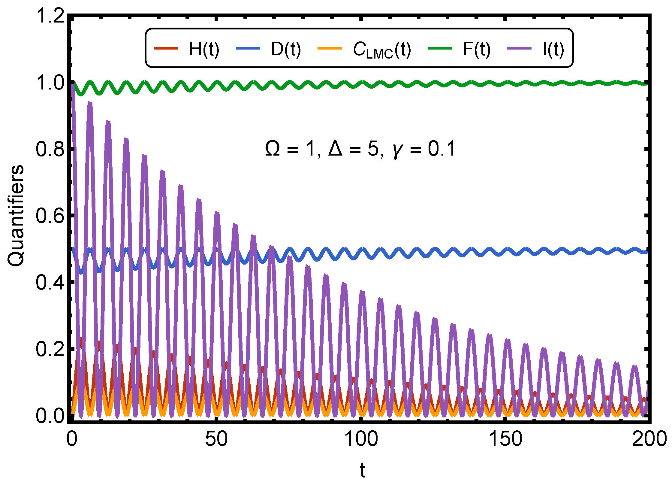
Figure 2.
Overdamped case: Time evolution of Shannon entropy (red), disequilibrium (blue), Complexity (Orange), fidelity (green), and quantum Fisher information (purple) for a overdamped Rabi oscillator. The parameters are normalized by setting ; the detuning is , and the damping rate is . The time variable is expressed in units of , so that t is dimensionless.
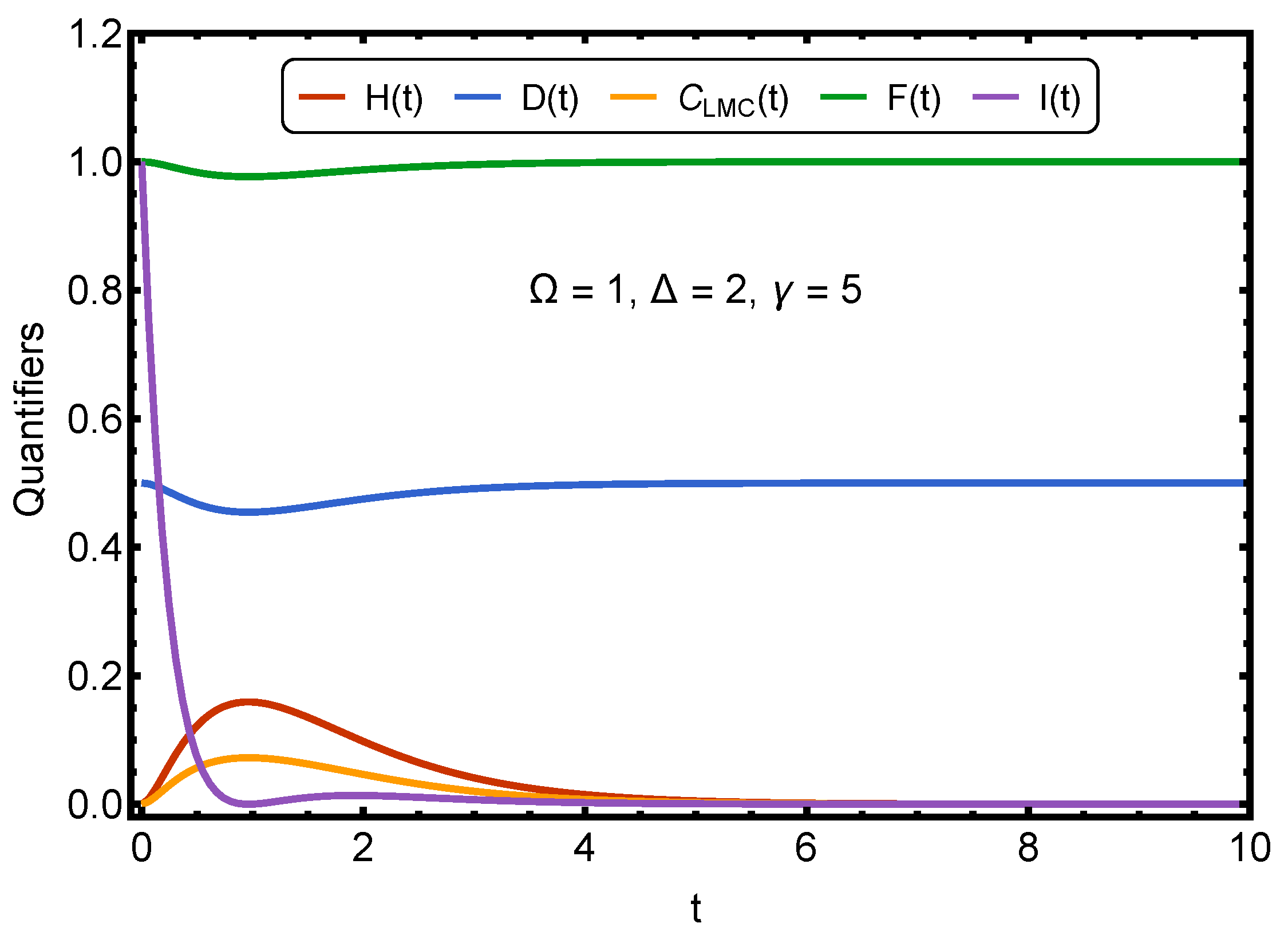
Figure 3.
Resonant case: Time evolution of Shannon entropy (red), disequilibrium (blue), Complexity (Orange), fidelity (green), and quantum Fisher information (purple) for a resonant Rabi regime. The parameters are normalized by setting ; the detuning is , and the damping rate is . The time variable is expressed in units of , so that t is dimensionless.
Disclaimer/Publisher’s Note: The statements, opinions and data contained in all publications are solely those of the individual author(s) and contributor(s) and not of MDPI and/or the editor(s). MDPI and/or the editor(s) disclaim responsibility for any injury to people or property resulting from any ideas, methods, instructions or products referred to in the content. |
© 2025 by the authors. Licensee MDPI, Basel, Switzerland. This article is an open access article distributed under the terms and conditions of the Creative Commons Attribution (CC BY) license (http://creativecommons.org/licenses/by/4.0/).
Copyright: This open access article is published under a Creative Commons CC BY 4.0 license, which permit the free download, distribution, and reuse, provided that the author and preprint are cited in any reuse.


