
Submitted:
15 December 2025
Posted:
16 December 2025
You are already at the latest version
Abstract
The constant growth of IP data traffic, driven by sustained annual increases surpassing 26%, is pushing current optical transport infrastructures towards their capacity limits. Since the deployment of new fiber cables is economically demanding, ultra-wideband transmission is emerging as a promising costly-effective solution, enabled by multi-band amplifiers and transceivers spanning the entire low-loss window of standard single-mode fibers. In this scenario, an accurate modeling of the frequency-dependent fiber parameters is essential to reliably model optical signal propagation. In particular, the combined impact of attenuation slope and inter-channel stimulated Raman scattering (SRS) fundamentally shapes the power evolution of wide wavelength division multiplexing (WDM) combs and directly affects nonlinear interference (NLI) generation. In this work, a set of analytical approximations for the frequency-dependent attenuation and Raman gain coefficient is presented, providing an effective balance between computational efficiency and physical fidelity. Through extensive simulations covering C, C+L, and ultra-wideband U-to-E transmission scenarios, the accuracy in reproducing the behavior of the power evolution and NLI profiles of fully numerical SRS models with the proposed approximations is demonstrated.
Keywords:
Inter-channel stimulated Raman scattering
; Single-mode optical fiber
; Frequencydependent loss coefficient
; Raman-aware NLI estimation
1. Introduction
The growth in demand for IP data traffic is expected to continue steadily, with authoritative mid-term forecasts indicating a compound annual growth rate of worldwide over the decade 2023-2033, and even higher values in specific network segments [1]. The deployment of coherent dual-polarization optical technologies in conjunction with Wavelength Division Multiplexed (WDM) systems has become crucial to support the transmission of such volumes of information beyond traditional core and metro-networks, for 5G x-haul transport [2], and for inter- and intra-datacenter connectivity. In this context, the evolution of the optical fiber infrastructure is fundamental to maintain the increasing traffic load while minimizing the need for new deployments, which would require substantial investments in CAPEX due to the high cost of new cables installation [3].
The standard single mode fiber (SSMF) made of purified glass (ITU-T G.652D fiber) [4] is currently the most deployed fiber variety, since it exhibits low attenuation (below 0.4 dB/km) within the single-mode transmission window, and no pronounced water-absorption peaks. This infrastructure covers the U, L, C, S, E and O bands, providing an available spectral window exceeding 50 THz, which represents an attractive solution to increase the overall transmission capacity while maximizing the return on existing CAPEX investments [4,5].
Currently, the C-band is the most widely used by commercial systems, providing 5 THz of the usable transmission bandwidth, while both showing the minimum attenuation of the SSMF and supporting erbium-doped fiber amplification (EDFA). However, C+L multiband solutions are already available [6], supported by Raman amplification and modern EDFAs extended to the L-band, allowing the exploitation of an additional 5 THz bandwidth [7].
In the multi-band optical network scenario, an extension of the classical physical-layer transmission models is necessary to incorporate the frequency dependence of the key fiber parameters, i.e, attenuation, chromatic dispersion and effective area, which influence the strength of nonlinear effects [5,9,13,24]. The dominant nonlinear mechanisms are the Kerr effect, responsible for nonlinear interference (NLI) noise [25,26], and stimulated Raman scattering (SRS), which transfers optical power from higher to lower frequencies by exciting inelastic resonances [19]. SRS plays the primary role in inter-band interactions and has a stronger impact on multiband transmission performance than the Kerr effect [10], therefore an accurate modeling is essential to find the optimum working point.
Raman scattering arises from the inelastic interaction between the optical field and the vibrational modes of the silica lattice [12,19]. In its spontaneous form, individual photons can transfer part of their energy to molecular vibrations, generating scattered light at lower frequencies (Stokes components). Even though each event is weak, in a WDM system, the aggregate effect over long propagation distances leads to spectral power tilt, with high frequency channels acting as energy donors while low frequency channels accumulate additional power. At high optical powers the effect becomes relevant, contributing both to nonlinear noise and Raman amplification.
SRS must be studied with respect to both the frequency and the propagation axis z, as the SRS-induced modification of the fiber loss/gain profile vs. z, for each frequency f, significantly affects the amount of NLI noise. Since the approximation of nonlinear propagation impairment as additive Gaussian noise [13] has been shown to hold even for low-dispersion fibers [14], perturbative NLI models can be extended across the entire U-to-E-band spectrum and partially into the O-band [5].
In this work, we focus our analysis to U-to-E-band scenarios on ITU-T G.652D fiber where the perturbative modeling for the NLI is solidly usable.
When transmission is limited along the C-band, SRS can be modeled as a spectral tilt [11], with the powers involved in the process decreasing proportionally to the total power. However, this approximation becomes increasingly inaccurate as the transmission bandwidth is expanded [27], and it eventually breaks down completely when the spectral occupation exceeds the SRS efficiency peak, located at roughly 13 THz [5]. For this reason, the set of ordinary differential equations (ODEs) [12,16] representing the SRS mathematical model must be solved numerically with non-negligible computational cost.
Despite the substantial progress made in modeling Raman interactions in optical fibers, accurately predicting the SRS-induced power evolution in wideband WDM transmission remains computationally demanding. Numerical integration of the full set of coupled ODEs provides a high-fidelity representation of the phenomenon [16], but its complexity poses a challenge for real-time optimization, online quality-of-transmission estimation, and large-scale network control. As multi-band systems extend well beyond the C+L bands and approach the full U-to-E operational window, there is a growing need for simplified, yet reliable, analytical approximations capable of retaining physical accuracy while reducing computational cost.
In this work, we address this need by systematically evaluating a set of Raman-gain approximations, derived through different curve-fitting strategies of the fiber Raman gain spectrum, and quantifying how these approximations impact the accuracy of the predicted power evolution along both the frequency and spatial axes. By replacing the exact Raman gain function with its fitted counterparts within the numerical SRS solver, we assess the resulting power error for a wideband multi-band scenario. This enables us to identify simplified descriptions of Raman interactions that preserve the essential physics while offering substantial reductions in complexity—thus providing a practical and efficient modeling tool for future ultra-wideband optical networks.
In addition to the Raman gain spectrum, other fiber parameters, most importantly the frequency-dependent attenuation, also require careful modeling across extremely wide spectral spans. Since the attenuation profile departs significantly from a flat behavior outside the C-band, this work also considers simplified representations of the loss coefficient obtained either through parametric fitting or by exploiting Taylor-series expansions around suitable reference frequencies. These approximations offer an additional opportunity to reduce the overall computational burden, while preserving the essential features required for accurate multi-band transmission analysis.
The remainder of this paper is organized as follows. In Section 2, we introduce the frequency-dependent single-mode fiber model adopted in this work, detailing the analytical description of the loss coefficient, effective area and Raman gain efficiency, and we present the proposed approximations for and based on piecewise–linear and Taylor–series fitting for attenuation and Gaussian/Lorentzian decompositions for the Raman gain. The numerical SRS solver, the considered multi-band transmission scenarios, and the error metrics used for validation, including RMSE on both power and NLI profiles, are also described. Section 3 reports the numerical results obtained for C, C+L, and ultra-wideband U-to-E transmission, comparing the different approximation strategies against the fully physical reference model in terms of power evolution and NLI accuracy. In Section 4, these results are critically discussed, highlighting the trade-offs between model complexity and accuracy and identifying the most effective combinations of attenuation and Raman-gain approximations for wideband QoT estimation. Finally, Section 5 concludes the paper by summarizing the main findings and outlining how the proposed modeling framework can support efficient physical-layer design, performance evaluation and network planning in future ultra-wideband optical networks.
2. Materials and Methods
In the following subsections, the main fiber parameters are presented, particularly highlighting their frequency dependence during optical propagation in a generic wideband transmission scenario.
The analysis assumes transmission over a SSMF having frequency-dependent spectral characteristics, i.e., attenuation, chromatic dispersion, effective area and Raman gain efficiency. The frequency bounds of each band composing the entire transmission scenario are presented in Table 1.
2.1. Loss Coefficient Function
The fiber loss coefficient models the power loss that affects the propagation of optical signals. It is obtained as the sum of different contributions deriving from the fiber composition and the manufacturing process, i.e., Rayleigh scattering, violet and infrared absorption, OH-ion absorption and phosphorous absorption in the fiber core. According to [17] the loss coefficient function vs. wavelength can be expressed in logarithmic units (dB/km) by modeling each phenomenological component as follows:
where:
The parameters A, B, , , adopted in this work, namely , , , , are taken from [18], where they are obtained through a dedicated fitting procedure applied to experimentally measured attenuation data. Figure 1 shows the comparison between the measured loss-coefficient samples and the corresponding fitted attenuation curve.
2.2. Loss Coefficients Approximations
While the full analytical expression of the loss coefficient reported in Equation (1) provides an accurate description of all physical contributions to fiber attenuation, its direct adoption in numerical simulations may lead to a substantial computational overhead. To mitigate this issue, two simplified yet effective approximations have been adopted in this work: a piecewise–linear fitting of the loss profile, and a Taylor–series expansion of each analytical term. Both strategies offer a significant reduction of the computational load while preserving the essential spectral behavior of , making them well suited for wideband propagation modeling.
2.2.1. Piecewise–Linear Approximation
In the first approximation, the measured attenuation profile is reconstructed as the sum of a set of linear segments. Let be a set of sampling points of the loss coefficient. The piecewise–linear approximation is defined as:
This representation can be interpreted as the sum of independent linear basis functions (segments), each active over a different wavelength interval. Despite its simplicity, the model closely matches the measured attenuation profile and is particularly suited for simulations requiring frequent evaluations of , such as wideband GN-model computations.
Figure 2 shows the agreement between the measured loss coefficient curve and the attenuation profile obtained through Piecewise-Linear Approximation.
2.2.2. Taylor–Series Approximation
A second approximation is obtained by expanding each analytical component of the attenuation model into a Taylor series around a reference wavelength (typically chosen near the center of the operating band). For a generic contribution (e.g., Rayleigh scattering, UV absorption, IR absorption), we consider:
retaining the first two or three terms depending on the smoothness of the underlying function.
The overall Taylor–based approximation of the attenuation is then:
where the index k spans all physical contributions included in the full model.
This approach produces a smooth analytical approximation (see Figure 3) that is computationally lightweight and particularly advantageous when must be evaluated inside integrals or differential equations.
2.3. Effective Area
The effective area is the parameter governing the strength of non linear interactions in optical fibers [12], as it quantifies the spatial confinement of the propagating mode. It is directly related to the nonlinear coefficient through (5):
where denotes the nonlinear refractive index of silica and the wavelength associated with the optical frequency f. A smaller effective area leads to higher optical field intensities, thereby enhancing Kerr-induced effects as well as Raman interactions.
Typically, in SSMF is not constant across the transmission bandwidth, and exhibits a slow frequency dependence, which becomes particularly non-negligible in wide-band transmission regimes.
If the modal profile can be approximated by a Gaussian function with radius , can be computed as , with , where a represents the fiber core radius and V is the normalized frequency, which can be expressed with relation (6). In the case of minor relative index step at the core-cladding interface, , where and represent the core and the cladding radius respectively. In this work a and are assumed to be equal to and , as for common SSMF, while the cladding refractive index and the refractive index difference with respect to the core are fixed at 1.45 and 0.31%.
2.4. Raman Gain Efficiency
The SRS is the principal nonlinear effect arising during multi-band transmission [20]. It originates from the inelastic interaction between the propagating electromagnetic field and the fiber’s dielectric medium. During Raman scattering, light incident on a medium is converted to a lower frequency. The energy difference of the signals at the two different frequencies determines the frequency shift and the Raman gain curve [12]. The Raman gain coefficient, , quantifies the coupling between the higher frequency () and lower frequency () channels, which are referred to as pump and Stokes wave respectively, and whose frequency shift is equal to . The power evolution of a signal propagating at frequency in the presence of SRS can be expressed through Equation (7),
where is the frequency-dependent attenuation coefficient.
Given a reference pump at the frequency , the whole Raman gain coefficient can be modeled with Equation (8)
where
is the Raman gain coefficient profile for a single fiber in terms of optical power, depending on , the Raman gain coefficient in terms of mode intensity, and the effective area overlap between the pump and the Stokes wave.
2.5. Raman Gain Approximations and Fitting Strategies
The Raman gain coefficient is characterized by a broadband and highly asymmetric spectral profile, as shown in Figure 4, with a main peak around 13 THz and a slowly decaying tail extending beyond 20 THz. The choice of a proper accurate and computationally efficient representation is fundamental when solving the SRS equations because it directly influences the inter-channel power transfer in wideband WDM systems.
In this work, several approximation strategies for are investigated, aiming to reduce numerical complexity while preserving physical fidelity. By exploiting analytical fits, the measured spectrum is approximated using parametric functions, i.e., combinations of Gaussian and Lorentzian profiles [15]. The accuracy of the result depends on the number of parameters and on the fitting bandwidth, making it possible to choose the suitable compromise between complexity and precision. Each approximation is incorporated in the SRS solver [22] and combined with the different approximations of to investigate the resulting power evolution across frequencies and space, and the error with respect to the reference model.
Two families of fitting functions are considered:
-
Gaussian decompositionThe Raman gain profile is approximated as the sum of a set of Gaussian functions:where the set of parameters is obtained through least squares procedure.Figure 5 illustrates the fitting result obtained using a set of eleven Gaussian basis functions, whose parameters are shown in Table 2. The ratio between the area of the fitted curve and that of the reference Raman-gain profile differs by only 0.07%, confirming the ability of Gaussian components to accurately reproduce both the main peak and the extended spectral tail.
-
Lorentzian decompositionThe Raman gain profile is approximated as the sum of a set of Lorentzian functions:where again the set of parameters (, ), representing the peak position and the full width at half maximum respectively, is obtained through the same least-squares fitting procedure used for the Gaussian decomposition.Figure 6 shows the Lorentzian-based fitting obtained with nine components (see Table 3). The resulting approximation closely matches the reference Raman-gain curve, with an area deviation of only %, demonstrating that Lorentzian bases also provide a flexible and accurate analytical representation of both the peak region and the long spectral tail.
2.6. Numerical SRS Solver
Optical power propagation along the fiber is numerically solved through the first-order differential equation modeling the SRS in the presence of fiber attenuation. For a single channel i, the differential equation can be expressed as Equation (12):
where
- = i-th channel power at distance z,
- = i-th channel attenuation coefficient,
- = Raman coefficient accounting for the power transfer from channel j to channel i
- = Raman gain induced on channel i from the other channels.
The numerical solver implements the discretized equation, obtained via explicit Euler method, according to Equation (13):
where L(z) accounts for the lumped losses and is the spatial step.
The coefficients in Equation (13) with the approximations described in the previous sections. In particular. The Raman interaction term is computed either using the experimental data or one of its analytical decompositions. Each approach generates a matrix of Raman coefficients which is directly injected in the solver without modifying the numerical scheme.
The same procedure is also applied for the attenuation coefficient , which can be evaluated using either the full physical loss model or one of its simplified representations.
As a result, the solver provides a unified framework in which different analytical models of both Raman gain and fiber attenuation can be consistently compared in terms of their impact on the power evolution along the span.
2.7. Simulation Setup
To test the errors induced by different approximations on both the received power profile and the amount of NLI, transmission systems using multiple bands have been analyzed by using the open-source tool GNPy [21,23]. As a reference, fiber loss and SRS profile from experimental data have been used, then the same analyses have been performed by feeding GNPy with the analyzed analytical approximations.
The numerical analysis is performed considering a multi-band WDM transmission system composed of 10 fiber spans 70 km long. The setup, illustrated in Figure 7, considers five spectral bands, i.e., U-, L-, C-, S-, E-band, with all the channels carrying an independent WDM signal. Reconfigurable optical add & drop multiplexers (ROADMs) are used to combine all the channels at the transmitter side, and then to launch the signal into the fiber spans. At the end of each span, channels are demultiplexed and signals are amplified through band-specific optical amplifiers. ROADMs are used again at the receiver side to route each wavelength to its dedicated optical receiver chain.
2.8. Validation Metrics and Error Definition
In order to quantify the accuracy of the proposed approximations of and , the error profiles on both the power and the Non Linear Interference (NLI) profiles have been computed according to respectively Equations (14) and (15):
where and represent respectively the reference and the approximated power profile, while and the reference and the approximated NLI profiles.
Due to the limitations in representing error profiles that depend on both frequency and distance along the link, an aggregated metric, the Root Mean Square Error (RMSE), has also been computed to provide a single summary value of the approximation accuracy for both the power and the NLI. The implemented formulas are:
where and represent the total numbers of frequency and space points along the link.
Although the RMSE does not capture all local variations of the errors across frequency and space, it offers a useful averaged measure to assess the overall quality of the power and NLI profiles across different transmission scenarios.
3. Results
To validate the results of the proposed approximations introduced in the previous sections, Equation (13) has been solved using the experimentally measured fiber attenuation and Raman gain coefficients . This provides a reference two-dimensional power profile in the frequency–distance domain, against which all the approximated models are compared. The following different transmission scenarios have been investigated considering a constant step of 0.8 m, and an injected input power per channel equal to 1 mW:
- C-band,
- L+C-band,
- L+C+S-band,
- L+C+E-band,
- U+L+C+S+E-band.
Then the reference profile has been compared with all the solutions obtained considering the following different combinations of the approximations of and :
- CASE 1: Piecewise-linear approximation of , experimental
- CASE 2: Taylor expansion of , experimental
- CASE 3: Experimental , gaussian fitting of
- CASE 4: Experimental , lorentzian fitting of
- CASE 5: Piecewise-linear approximation of , gaussian fitting of
- CASE 6: Piecewise-linear approximation of , lorentzian fitting of
- CASE 7: Taylor expansion of , gaussian fitting of
- CASE 8: Taylor expansion of , lorentzian fitting of
The RMSE of the power profiles has been computed and reported in Table 4:
The RMSE of the NLI profiles has been also computed and reported in Table 5:
To complement the RMSE-based analysis, illustrate respectively the output signal power output signal power and frequency-dependent Non-Linear Interference (NLI) power at the end of the transmission system before final signal amplification, for CASE 5, 6, 7, 8, which combine the approximations of both and . These results provide a direct comparison between the most approximated models and the fully physical reference solution, highlighting how the different representations of and influence the final system-level performance.
In both figures, each curve corresponds to one of the approximation cases. The NLI spectra allow quantifying how inaccuracies in the modeling propagate to the nonlinear domain, while the output power profiles show the cumulative effect of Raman interactions and attenuation along the span. The visual comparison enables identifying regions of the spectrum that are more sensitive to modeling errors, and evaluating whether some approximations introduce systematic deviations or only small perturbations with respect to the reference profile.
Figure 8.
Output power [dBm] at the end of the transmission system in the U-L-C-S-E-band scenario.
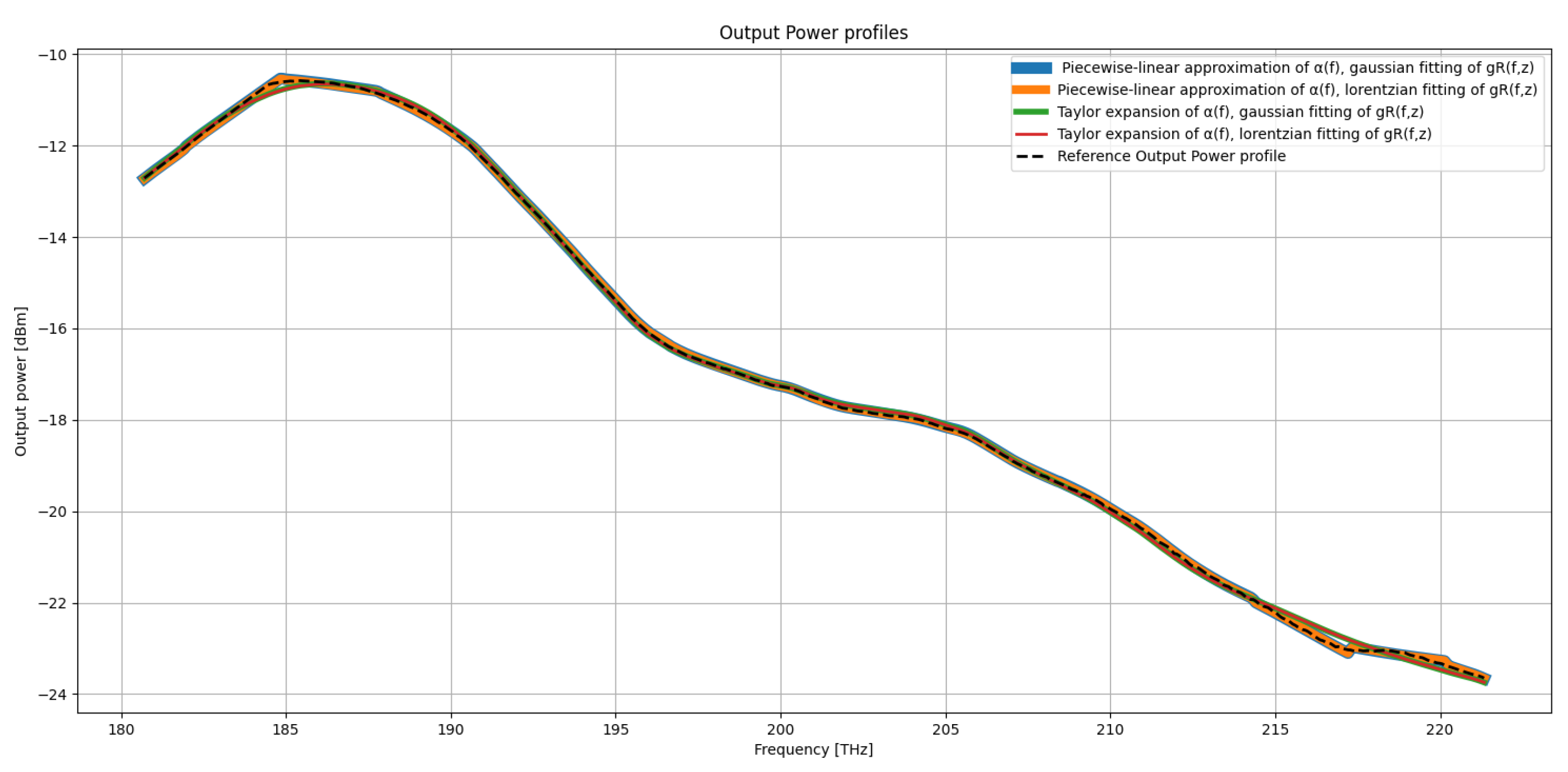
Figure 9.
Output NLI [dBm] at the end of the transmission system in the U-L-C-S-E-band scenario.
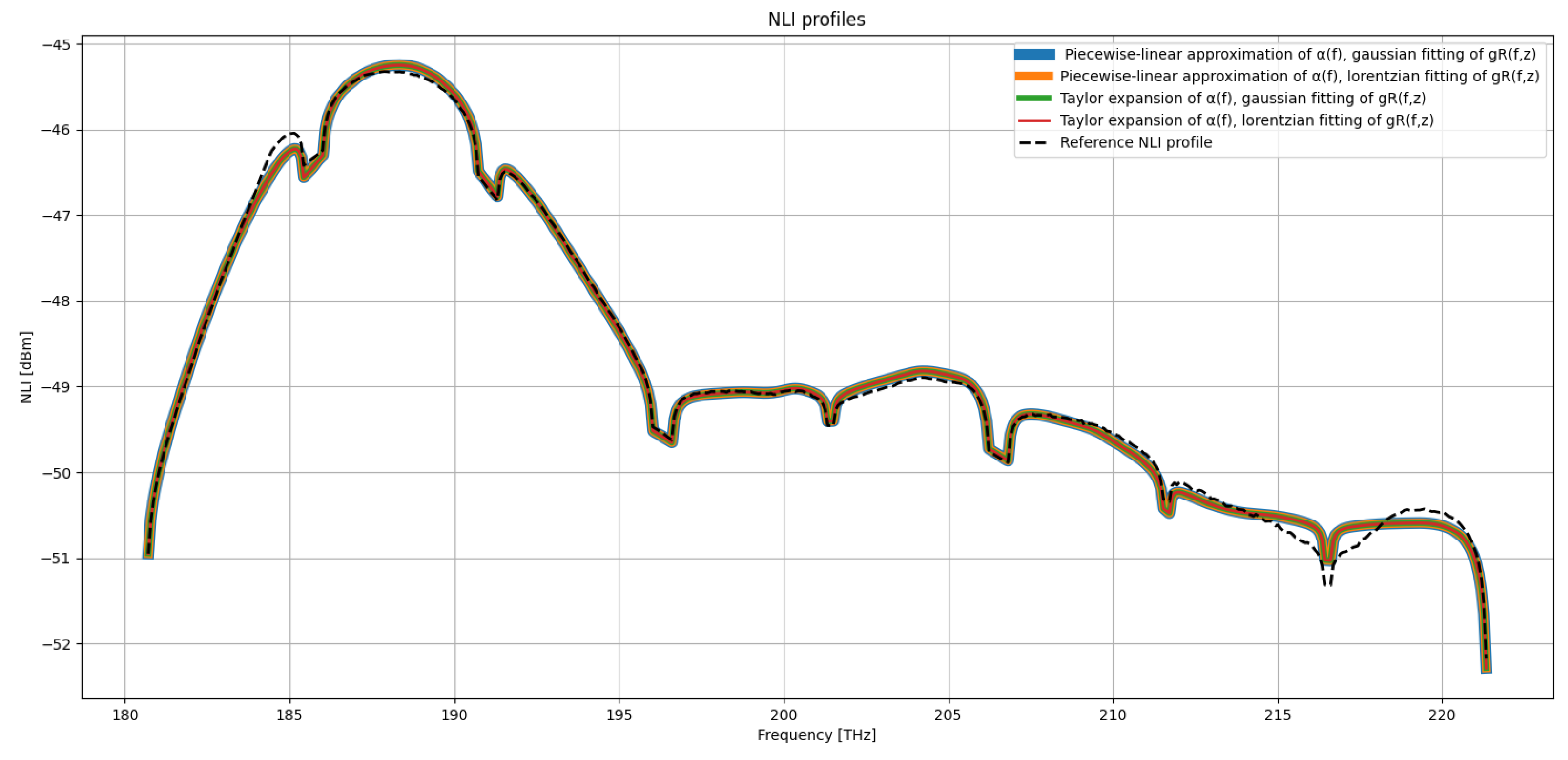
Figure 10.
Power error [dB] along the line in the U-L-C-S-E-Band transmission scenario for the following cases: (a) Piecewise-linear approximation of , gaussian fitting of . (b) Piecewise-linear approximation of , lorentzian fitting of .
Figure 10.
Power error [dB] along the line in the U-L-C-S-E-Band transmission scenario for the following cases: (a) Piecewise-linear approximation of , gaussian fitting of . (b) Piecewise-linear approximation of , lorentzian fitting of .
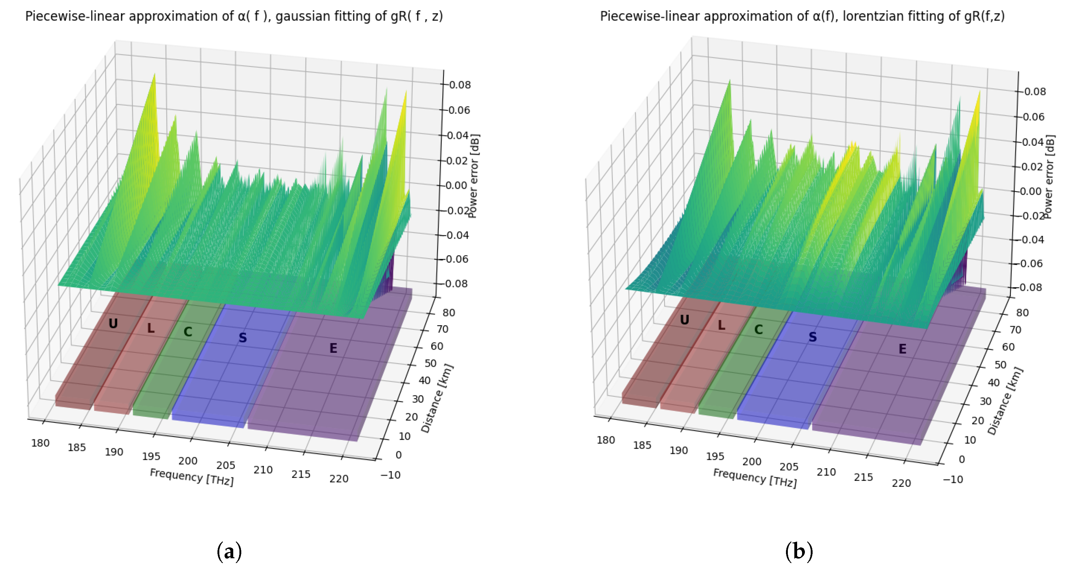
Figure 11.
Power error [dB] along the line in the U-L-C-S-E-Band transmission scenario for the following cases: (a) Taylor expansion of , gaussian fitting of . (b) Taylor expansion of , lorentzian fitting of .
Figure 11.
Power error [dB] along the line in the U-L-C-S-E-Band transmission scenario for the following cases: (a) Taylor expansion of , gaussian fitting of . (b) Taylor expansion of , lorentzian fitting of .
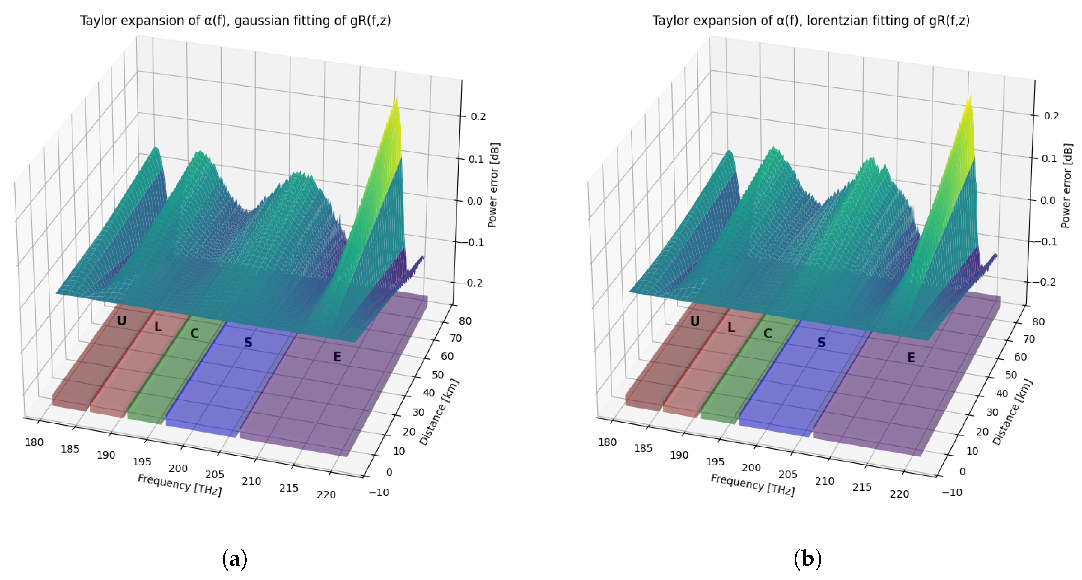
Beyond the scalar RMSE indicators, it is instructive to observe how the approximation errors distribute over the frequency–distance plane. The following 3D error maps provide a qualitative representation of the deviation from the reference solution for the fully approximated models in the U-,L-,C-,S-,E-band transmission scenarios. Although such plots do not allow for fine-grained quantitative comparison—owing to the inherent limitations of projecting dense numerical data onto a surface—they offer valuable insight into the spatial and spectral patterns of the modeling inaccuracies, making explicit where each approximation tends to accumulate error along the span.
4. Discussion
The comparison between the approximated models and the fully physical reference solution highlights the impact of the different decomposition and fitting strategies for both and on the accuracy of the predicted power evolution and the resulting NLI generation across all transmission bandwidths.
Overall, the results indicate that the piecewise-linear representation of the attenuation profile (CASE 1, 5, 6) systematically outperforms the Taylor-series-based approximation (CASE 2, 7, 8). This suggests that the local linearization of is more suitable for capturing the frequency-dependent attenuation behaviour over ultra-wideband spectra, especially in the presence of rapid spectral variations.
Regarding the Raman gain coefficient approximations, the Lorentzian fit (CASE 4, 6, 8) consistently achieves lower RMSE values compared to the Gaussian fit (CASE 3, 5, 7). This outcome is aligned with the intrinsic asymmetric shape and spectral tails of the experimentally measured Raman gain curve, which are better reproduced by a Lorentzian model. This is also coherent with the area-overlap analysis performed earlier, where the Lorentzian decomposition yielded a closer match to the measured gain distribution.
Among all tested combinations, CASE 4, combining the experimental with a Lorentzian fitting of , provides the highest overall accuracy for both the SRS power-profile prediction and the corresponding NLI estimation across all bandwidth scenarios.
When extending the transmission bandwidth from C → L+C → L+C+S → L+C+E → U+L+C+S+E, a consistent trend emerges across all configurations. First, both the SRS and NLI metrics exhibit a general increase in RMSE. Second, the system becomes progressively more sensitive to the adopted approximations, as the spectral profiles of and become increasingly structured and therefore more challenging to model accurately.
This behavior is expected: as the transmission bandwidth widens, the physical interactions, particularly Raman coupling, occur across channels that are more widely separated in frequency. Consequently, higher model fidelity is required to correctly capture the underlying frequency-dependent Raman interactions.
The main error source is represented by the fitting of , and this directly influences the power evolution and, consequently, the NLI profile.
The overall behavior of RMSE is also confirmed by , which show a marginal impact of both the output power and the NLI. The deviations among the models remain below 0.1 dB, fully consistent with the RMSE values reported in Table 4 and Table 5, confirming that the solver retains high accuracy even under aggressive approximation schemes.
Additionally, the figure shows a clear maximum of NLI around 186–188 THz, corresponding to the region where the optical power is highest, and a progressive reduction of NLI towards the spectral edges, consistent with reduced Raman efficiency and increasing fiber attenuation.
Both the NLI and the output power profiles exhibit an excellent overlap across all approximation models. NLI generation is primarily governed by the spectral structure of the transmitted signal and by the power evolution along the link, rather than by the fine details of the Raman and attenuation approximations. This confirms that the proposed attenuation and Raman-gain approximations preserve the physical power evolution along the link and introduce only minor deviations in the computed non-linear interference. As expected, the spectral region around 186–188 THz shows the strongest interaction, while the spectral edges experience lower power and reduced NLI levels. Overall, the numerical results demonstrate the robustness of the proposed approximations and their suitability for wideband optical fiber modeling.
5. Conclusions
In this work, a systematic evaluation of simplified analytical models for the frequency-dependent attenuation and Raman gain coefficients in ultra-wideband optical transmission systems is presented. Different combinations of approximations are tested and compared against a fully physical reference model to quantify the accuracy and the impact on both power and non linear interference evaluation of the novel methodologies.
The study validates all the approaches, showing, in particular, slightly better results when using the piecewise–linear fitting of and the Gaussian decomposition of , especially when expanding from the C+L bands to the full U-to-E spectrum.
Overall, the presented study provides a practical framework for selecting appropriate attenuation and Raman approximations depending on the targeted operational bandwidth and accuracy requirements. These results can support the development of more efficient tools for physical-layer modeling, system optimization, and network-level planning in future ultra-wideband optical infrastructures.
Funding
This research was funded by the EU Horizon project SENSEI (GA: 101189545).
Data Availability Statement
Data and software used to obatin the presented results are openly available at https://github.com/Telecominfraproject/oopt-gnpy.
Conflicts of Interest
The authors declare no conflicts of interest.
Abbreviations
The following abbreviations are used in this manuscript:
| WDM | Wavelength Division Multiplexing |
| SSMF | Standard Single Mode Fiber |
| SRS | Stimulated Raman Scattering |
| NLI | Non Linear Interference |
| ODE | Ordinary Differential Equations |
| GN | Gaussian Noise |
| RMSE | Root Mean Square Error |
References
- Nokia. Nokia Global Network Traffic Repor. 2023. Available online: https://www.kgpco.com/userfiles/nokia_global_network_traffic_report_en.pdf (accessed on 12 December 2025).
- Al-Falahy, N.; Alani, O. Y. Technologies for 5G Networks: Challenges and Opportunities. IT Prof. 2017, 19, 12–20. [Google Scholar] [CrossRef]
- Lopez, V.; et al. Optimized Design and Challenges for C&L Band Optical Line Systems. J. Lightwave Technol. 2020, 38, 1080–1091. [Google Scholar]
- Ferrari, et al. Assessment on the Achievable Throughput of Multi-Band ITU-T G.652.D Fiber Transmission Systems. J. Lightwave Technol. 2020, 38, 4279–4291. [Google Scholar] [CrossRef]
- Hoshida, T.; et al. Ultrawideband Systems and Networks: Beyond C + L-Band. Proc. IEEE 2022, 110, 1725–1741. [Google Scholar] [CrossRef]
- Cantono, M.; et al. Opportunities and Challenges of C+L Transmission Systems. J. Lightwave Technol. 2020, 38, 1050–1060. [Google Scholar] [CrossRef]
- Rapp, L.; Eiselt, M. Optical Amplifiers for Multi–Band Optical Transmission Systems. J. Lightwave Technol. 2021, 40, 1579–1589. [Google Scholar] [CrossRef]
- Curri, V. Software-Defined WDM Optical Transport in Disaggregated Open Optical Networks. In Proceedings of the 22nd International Conference on Transparent Optical Networks (ICTON), 2020; pp. 1–4. [Google Scholar] [CrossRef]
- D’Amico, A.; et al. Scalable and Disaggregated GGN Approximation Applied to a C+L+S Optical Network. J. Lightwave Technol. 2022, 40, 3499–3511. Available online: https://opg.optica.org/jlt/abstract.cfm?URI=jlt-40-11-3499 (accessed on 12 December 2025). [CrossRef]
- D’Amico, A.; et al. Inter-Band GSNR Degradations and Leading Impairments in C+L Band 400G Transmission. In Proceedings of the 2021 International Conference on Optical Network Design and Modeling (ONDM), 2021; pp. 1–3. [Google Scholar] [CrossRef]
- Chraplyvy, A. R. Limitations on Lightwave Communications Imposed by Optical-Fiber Nonlinearities. J. Lightwave Technol. 1990, 8(10), 1548–1557. [Google Scholar] [CrossRef]
- Agrawal, G. P. Nonlinear Fiber Optics, 5th ed.; Academic Press: Boston, 2013. [Google Scholar]
- Semrau, D.; Bayvel, P. The Gaussian Noise Model in the Presence of Inter-Channel Stimulated Raman Scattering. J. Lightwave Technol. 2018, 36(1), 1–12. [Google Scholar] [CrossRef]
- Nespola, A.; et al. GN-Model Validation Over Seven Fiber Types in Uncompensated PM-16QAM Nyquist-WDM Links. IEEE Photonics Technol. Lett. 2014, 26(2), 206–209. [Google Scholar] [CrossRef]
- Hollenbeck, D.; Cantrell, C. D. Multiple-Vibrational-Mode Model for Fiber-Optic Raman Gain Spectrum and Response Function. J. Opt. Soc. Am. B 2002, 19(12), 2886–2892. [Google Scholar] [CrossRef]
- Tariq, S.; Palais, J. C. A Computer Model of Non-Dispersion-Limited Stimulated Raman Scattering in Optical Fiber Multiple-Channel Communications. J. Lightwave Technol. 1993, 11(12), 1914–1924. [Google Scholar] [CrossRef]
- Walker, S. Rapid Modeling and Estimation of Total Spectral Loss in Optical Fibers. J. Lightwave Technol. 1986, 4(8), 1125–1131. [Google Scholar] [CrossRef]
- D’Amico, A.; Borraccini, G.; Curri, V. Introducing the Perturbative Solution of the Inter-Channel Stimulated Raman Scattering in Single-Mode Optical Fibers. arXiv 2023, arXiv:2304.11756. [Google Scholar] [CrossRef]
- Stolen, R. H.; Gordon, J. P.; Tomlinson, W. J.; Haus, H. A. Raman Response Function of Silica-Core Fibers. J. Opt. Soc. Am. B 1989, 6(6), 1159–1166. [Google Scholar] [CrossRef]
- Bromage, J. Raman Amplification for Fiber Communications Systems. J. Lightwave Technol. 2004, 22(1), 79–93. [Google Scholar] [CrossRef]
- Telecom Infra Project. GNPy: Open-Source Tool for Physical Layer Modeling in Open Optical Networks. Available online: https://github.com/Telecominfraproject/oopt-gnpy.
- GNPy Documentation. Available online: https://gnpy.readthedocs.io/en/master/ (accessed on 12 December 2025).
- Curri, V. GNPy Model of the Physical Layer for Open and Disaggregated Optical Networking [Invited]. J. Opt. Commun. Netw. 2022, 14 (6), C92–C104. Available online: https://opg.optica.org/jocn/abstract.cfm?URI=jocn-14-6-C92 (accessed on 12 December 2025). [CrossRef]
- Cantono, M.; Pilori, D.; Ferrari, A.; Catanese, C.; Thouras, J.; Augé, J.-L.; Curri, V. On the Interplay of Nonlinear Interference Generation with Stimulated Raman Scattering for QoT Estimation. J. Lightw. Technol. 2018, 36(15), 3131–3141. [Google Scholar] [CrossRef]
- Poggiolini, P.; Bosco, G.; Carena, A.; Curri, V.; Jiang, Y.; Forghieri, F. The GN-Model of Fiber Non-Linear Propagation and Its Applications. J. Lightw. Technol. 2014, 32(4), 694–721. [Google Scholar] [CrossRef]
- Dar, R.; Feder, M.; Mecozzi, A.; Shtaif, M. Accumulation of Nonlinear Interference Noise in Fiber-Optic Systems. Opt. Express 2014, 22(12), 14199–14211. Available online: https://opg.optica.org/oe/abstract.cfm?uri=oe-22-12-14199 (accessed on 12 December 2025). [CrossRef] [PubMed]
- Souza, A.; Costa, N.; Pedro, J.; Pires, J. Comparison of Fast Quality of Transmission Estimation Methods for C+L+S Optical Systems. J. Opt. Commun. Netw. 2023, 15(1), F1–F12. Available online: https://opg.optica.org/jocn/abstract.cfm?uri=jocn-15-1-F1 (accessed on 12 December 2025). [CrossRef]
Figure 1.
SSMF wideband loss coefficient profile, [18].
Figure 1.
SSMF wideband loss coefficient profile, [18].
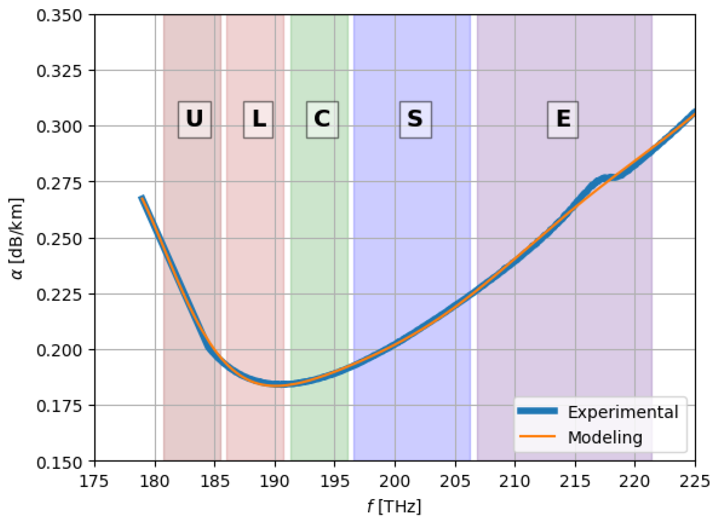
Figure 2.
SSMF attenuation profile obtained through Piecewise-Linear Approximation
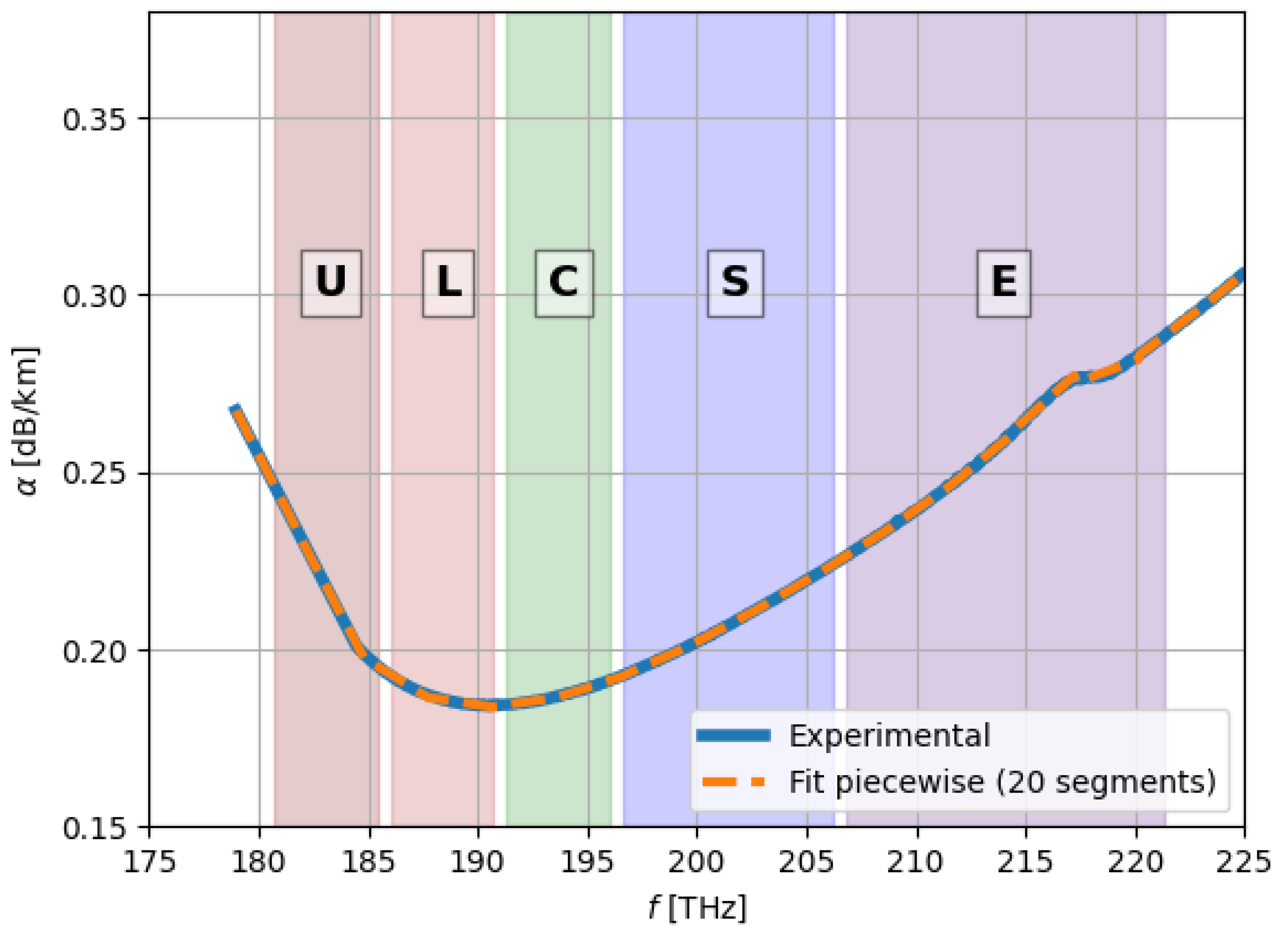
Figure 3.
SSMF attenuation profile obtained through Taylor-Series expansion of the analytical components in Equation (1)
Figure 3.
SSMF attenuation profile obtained through Taylor-Series expansion of the analytical components in Equation (1)
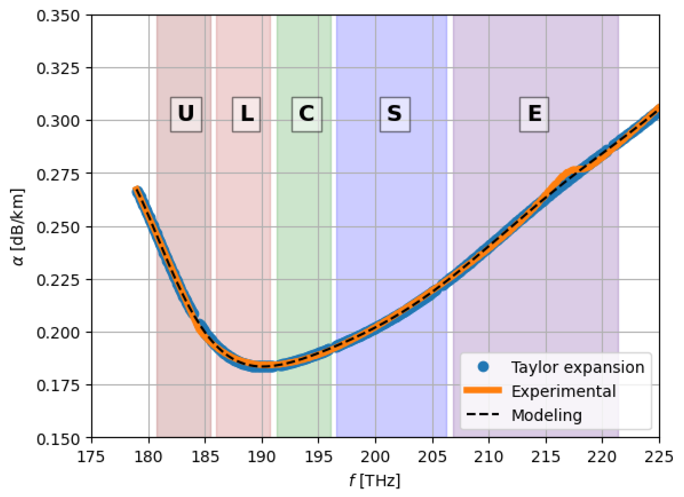
Figure 4.
SSMF Raman gain coefficient profile for each frequency of the considered wideband scenario [18].
Figure 4.
SSMF Raman gain coefficient profile for each frequency of the considered wideband scenario [18].
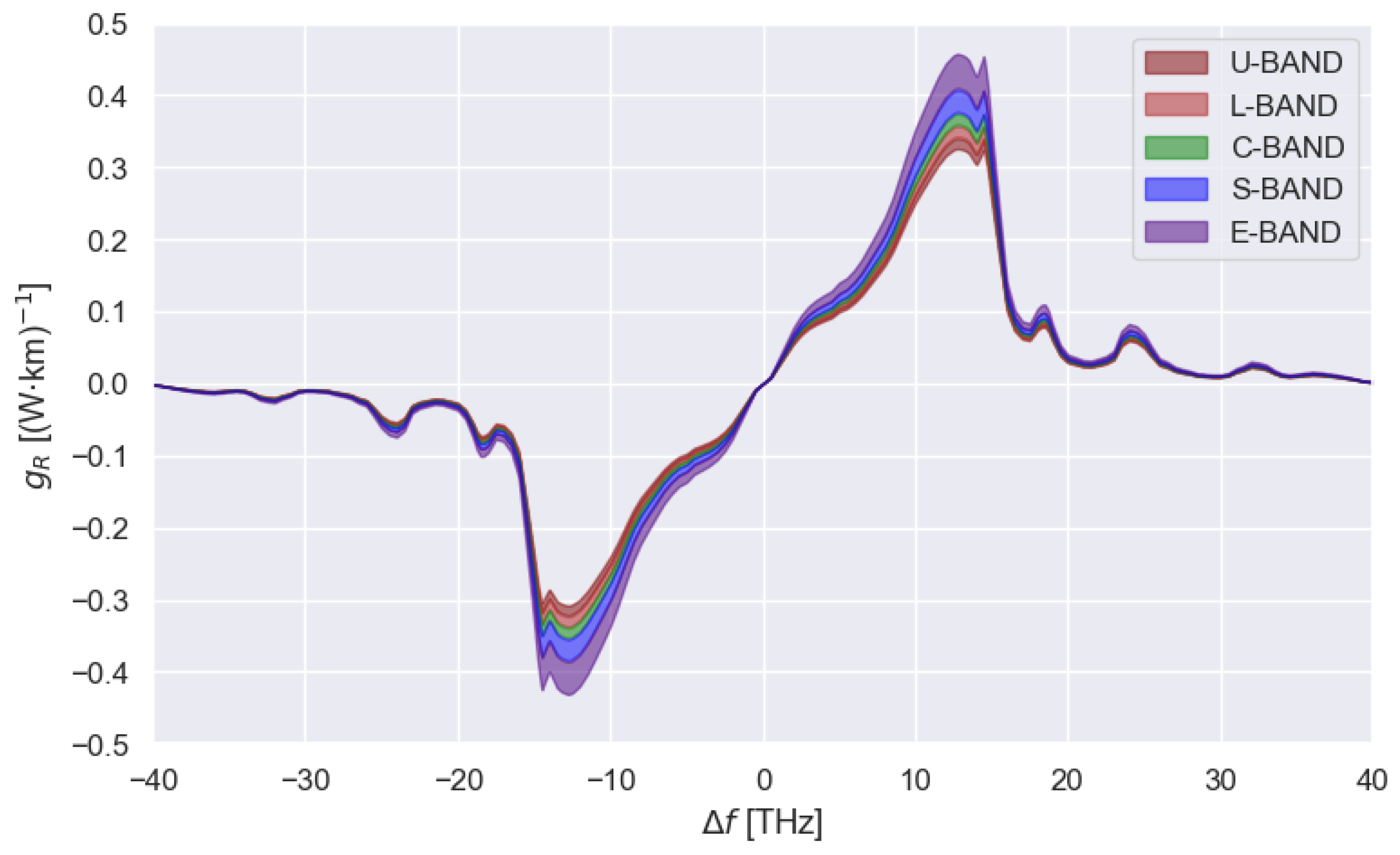
Figure 5.
SSMF Normalized Raman gain coefficient profile approximated through Gaussian decomposition
Figure 5.
SSMF Normalized Raman gain coefficient profile approximated through Gaussian decomposition
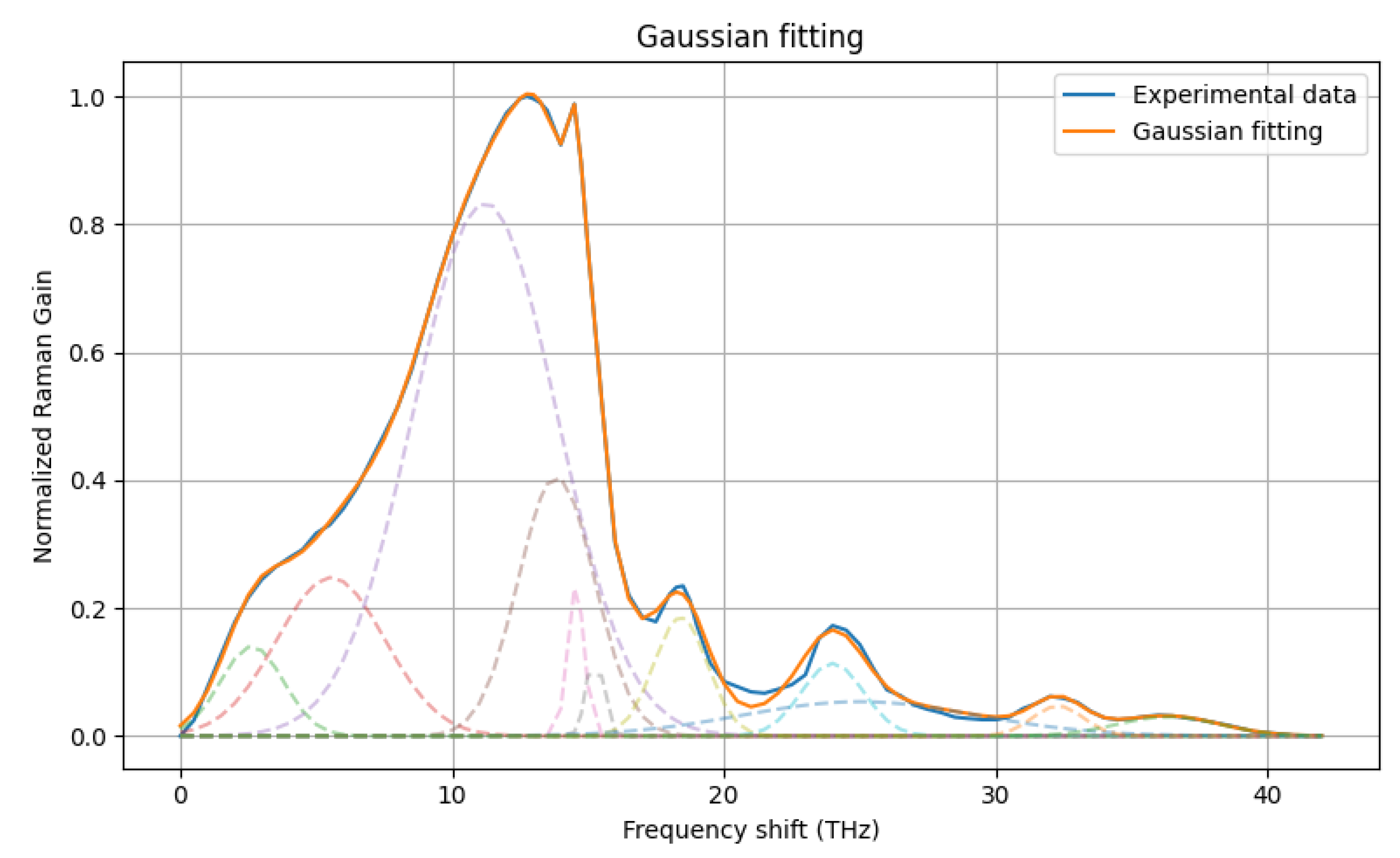
Figure 6.
SSMF Normalized Raman gain coefficient profile approximated through Lorentzian decomposition
Figure 6.
SSMF Normalized Raman gain coefficient profile approximated through Lorentzian decomposition
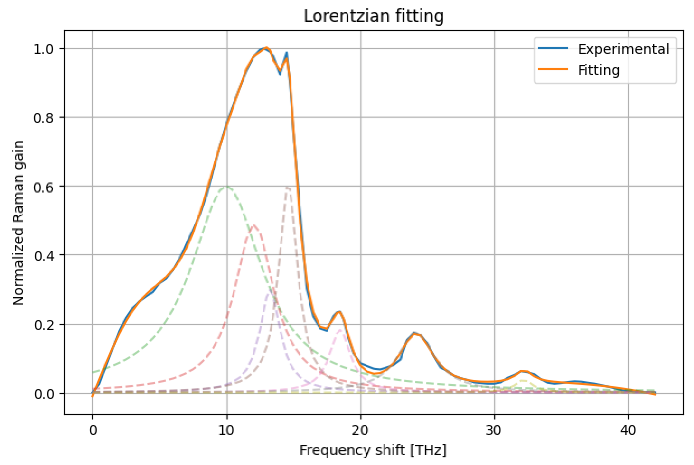
Figure 7.
Scheme of the implemented optical line system architecture
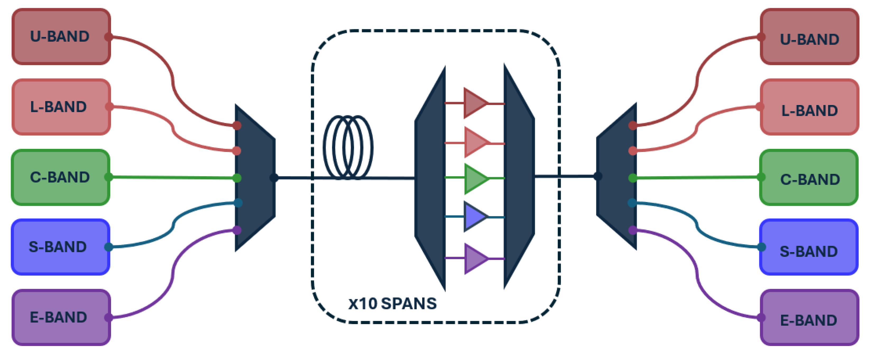

Table 1.
Frequency bounds and bandwidth of each band composing the entire transmission scenario.
| Band | (THz) | (THz) | Bandwidth (THz) |
|---|---|---|---|
| U | 180.710 | 185.510 | 4.800 |
| L | 186.010 | 190.810 | 4.800 |
| C | 191.310 | 196.110 | 4.800 |
| S | 196.610 | 206.210 | 9.600 |
| E | 206.810 | 221.210 | 14.400 |
Table 2.
Sets of parameters describing the eleven Gaussian basis functions
| (THz) | (THz) | |
|---|---|---|
Table 3.
Sets of parameters (, ) describing the nine Lorentzian basis functions.
| (THz) | (THz) |
|---|---|
| 3.1771 | 3.0137 |
| 0.2363 | 4.1563 |
| 10.0000 | 2.0315 |
| 0.2283 | 3.2216 |
| 12.0761 | 1.3648 |
| 0.1858 | 2.6805 |
| 13.2623 | 1.0037 |
| 0.1129 | 1.8794 |
| 14.6135 | 1.4891 |
| 0.2264 | 1.1439 |
| 18.4901 | 1.0539 |
| 0.0689 | 1.8113 |
| 24.1727 | 1.2816 |
| 0.0665 | 2.5900 |
| 32.2231 | 0.7614 |
| 0.0132 | 2.0680 |
| 36.6635 | 10.0000 |
| 0.6144 | 10.0000 |
Table 4.
RMSE of the power profiles computed in the different transmission scenarios expressed in dB.
Table 4.
RMSE of the power profiles computed in the different transmission scenarios expressed in dB.
| C-band | L+C-band | L+C+S-band | L+C+E-band | U+L+C+S+E-band | |
|---|---|---|---|---|---|
| CASE 1 | |||||
| CASE 2 | |||||
| CASE 3 | |||||
| CASE 4 | |||||
| CASE 5 | |||||
| CASE 6 | |||||
| CASE 7 | |||||
| CASE 8 |
Table 5.
RMSE of the Non Linear Interference (NLI) profiles computed in the different transmission scenarios expressed in dB.
Table 5.
RMSE of the Non Linear Interference (NLI) profiles computed in the different transmission scenarios expressed in dB.
| C-band | L+C-band | L+C+S-band | L+C+E-band | U+L+C+S+E-band | |
|---|---|---|---|---|---|
| CASE 1 | |||||
| CASE 2 | |||||
| CASE 3 | |||||
| CASE 4 | |||||
| CASE 5 | |||||
| CASE 6 | |||||
| CASE 7 | |||||
| CASE 8 |
Disclaimer/Publisher’s Note: The statements, opinions and data contained in all publications are solely those of the individual author(s) and contributor(s) and not of MDPI and/or the editor(s). MDPI and/or the editor(s) disclaim responsibility for any injury to people or property resulting from any ideas, methods, instructions or products referred to in the content. |
© 2025 by the authors. Licensee MDPI, Basel, Switzerland. This article is an open access article distributed under the terms and conditions of the Creative Commons Attribution (CC BY) license (http://creativecommons.org/licenses/by/4.0/).
Copyright: This open access article is published under a Creative Commons CC BY 4.0 license, which permit the free download, distribution, and reuse, provided that the author and preprint are cited in any reuse.


