
Submitted:
12 December 2025
Posted:
16 December 2025
You are already at the latest version
Abstract
A program package for calculating regularized classical trajectories for Coulomb n−body problem is developed. The Coulomb singularities from the equations of motion are removed by transformations of variables including the time. This effectively conserves the energy of the time-independent systems to a high accuracy for long time propagation. Sample calculations are shown for the cases of 2,3,4, and 5 particle systems giving comparisons with the un-regularized trajectories. The program can be used for general purposes including the classical-trajectory Monte-Carlo simulations for charged-particle collisions in free or laser environments.
Keywords:
Coulomb singularity
; n−body problem
; regularization
; atomic collisions
; laser-assisted processes
1. Introduction
The dynamics of charged particles interacting through the long-range Coulomb potential play a central role in many areas of physics, ranging from atomic and molecular collisions to plasma dynamics and astrophysical processes. However, the accurate numerical treatment of such systems remains a persistent challenge due to the singular nature of the Coulomb interaction at short inter-particle separations. In particular, direct integration of the classical equations of motion for few- and many-body Coulomb systems often leads to numerical instabilities or loss of energy conservation during close encounters of two or more particles. Overcoming these singularities is essential for constructing reliable trajectory-based simulations, specifically involving particles such as electrons and positrons.
Existing computational frameworks for charged-particle dynamics typically handle the Coulomb interaction either by introducing soft-core potentials, adaptive time steps, or cutoff distances to avoid singularities during close encounters. While such techniques can stabilize direct numerical integration, they do so at the cost of distorting the true Coulomb dynamics near short inter-particle separations. The true nature of the Coulomb potential at short distance is essential to accurately capture the dynamics in cases where, for example, an electron performs several encounters with an oppositely charged ion due to a laser field. It has been shown, that in laser-assisted collisions, the exact inclusion of the Coulomb potential between the electron and a proton leads to interesting phenomena [1,2,3,4,5] which are not observed if the Coulomb potential is softened. Some exact treatments of the Coulomb singularity include the treatment of frustrated ionization for strongly driven molecules in ref [6] and later analysis of double and triple ionization of three electron-atoms [7] and molecules [8], driven by infrared laser pulses.
In the present work, we introduce a general program to compute the classical trajectories in the charged particle system by globally regularizing the Coulomb singularities. It must be noted that the regularizing singular collisions in the body problem is not new, rather it has been extensively studied and successfully applied in the problem of gravitational body problem. See, for example, the classic texts by Aarseth [9] and Szebehely [10], and the references therein. More practical approach to computing regularized trajectories in the body gravitational problem is due to the works of Heggie [11] and Mikkola [12]. Therefore, we closely follow their derivations to arrive at the formula for the Coulomb system. In addition, we also introduce an oscillating electric field to the charged-particle system to address a larger class of problems in collisions physics.
The organization of the present paper is as follows. In Section 2 we derive our main equations, and in Section 3 we describe the main program nbodycl. For comparisons, we also provide a standard generalized integrator program called nbody-direct for the body Coulomb system without regularization. In Section 4 we compare the results from nbodycl and nbody-direct applied to example problems with number of charged particles and 5. Finally in Section 5 we discuss the additional challenges in the nbodycl program and its potential applications.
2. Formulation
For an n charged-particle system interacting with a time-dependent electric field, the system’s Hamiltonian in the dipole approximation can be written as,
where the canonical variables and are the Cartesian coordinate and its conjugate momentum of the particle. The mass and the charge of the particle are given by and , respectively. The form of the time-dependent electric field vector can be arbitrary. Note that we will be using atomic units meaning that for an electron (positron) and . The solution paths of Eq. (1) are given by the integration of Hamilton’s equations,
where the dot represent the time derivative with respect to t. The direct numerical integration of the Hamilton’s equations (Newton’s equations) in Eqs. (2) and (3) introduce severe numerical instabilities when two or more particles approach infinitesimally close to each other, i.e., when . These instabilities are commonly known as Coulomb singularities where the kinetic and potential energies of the system diverge. Therefore, we look for a global regularization for the Hamiltonian in Eq. (1) without Coulomb singularities.
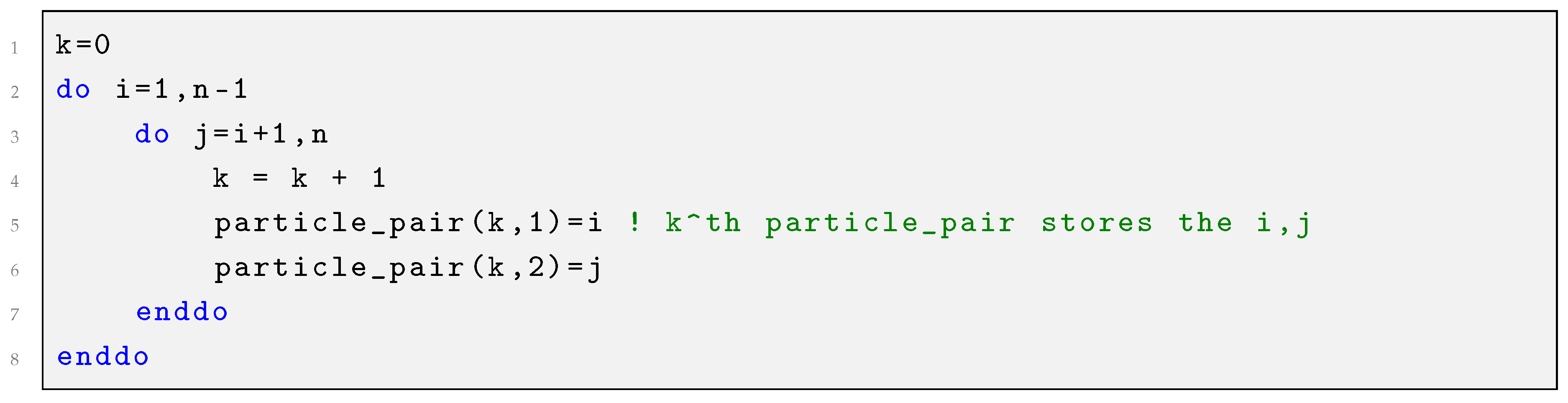
For the regularization, we introduce the new coordinate variable and its conjugate momentum for each pair of particles. For an n distinguishable particle system, there are distinct pairs of particles. We can count the particle pairs with index k as the following code snippet shows.
 We also note that the indices can be directly mapped to the index k via . The new coordinate variables are defined as follows,
where and . The inverse transformation for the coordinate variable can be obtained from Eqs. (4) and (5) to give,
The new conjugate momenta are given by,
Note that if we wish to stay in the center-of-mass frame, we can take and . As before, the inverse transformation for the conjugate momentum can be obtained from Eqs. (7) and () to give,
The inverse transformation in Eq. (9) can be recast into the following compact form,
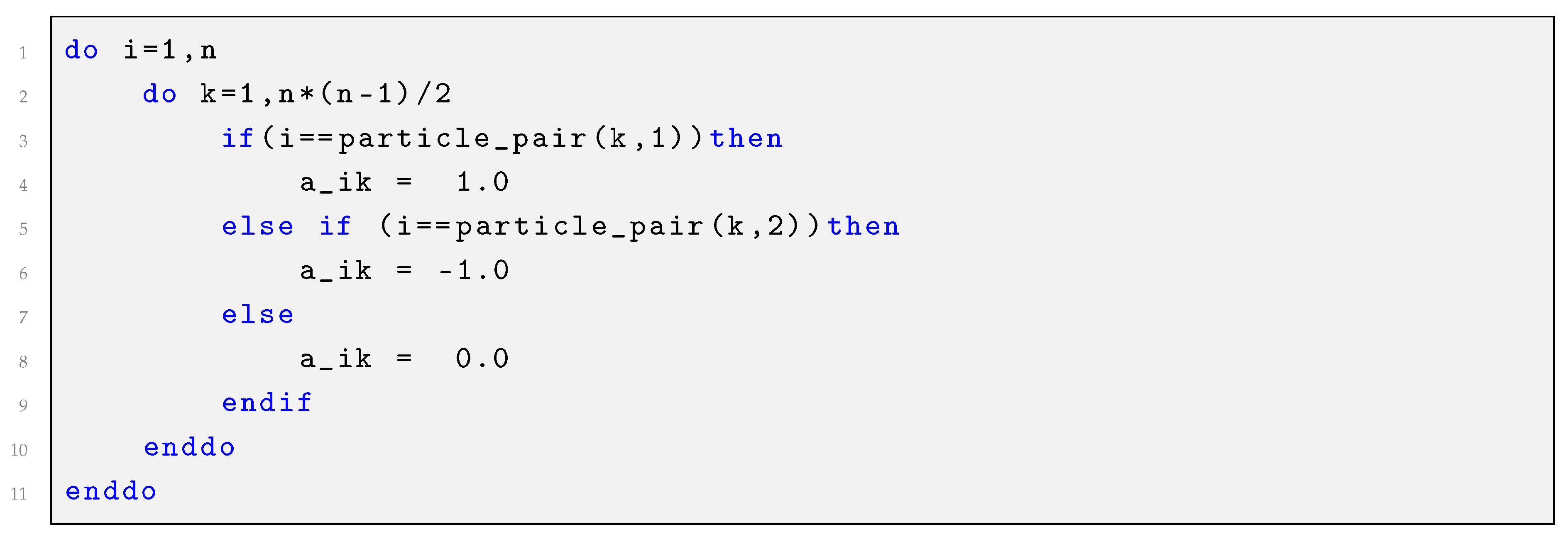
where , and when , otherwise . In other words (recall that index k refers to the pair of particles with ), if the particle i is the first index of the pair, then , and if the particle j is the second index of the pair, then , and finally, if the particle i is not included in the pair given by k, then . Following code snippet shows how the terms are calculated.
We also note that the indices can be directly mapped to the index k via . The new coordinate variables are defined as follows,
where and . The inverse transformation for the coordinate variable can be obtained from Eqs. (4) and (5) to give,
The new conjugate momenta are given by,
Note that if we wish to stay in the center-of-mass frame, we can take and . As before, the inverse transformation for the conjugate momentum can be obtained from Eqs. (7) and () to give,
The inverse transformation in Eq. (9) can be recast into the following compact form,
where , and when , otherwise . In other words (recall that index k refers to the pair of particles with ), if the particle i is the first index of the pair, then , and if the particle j is the second index of the pair, then , and finally, if the particle i is not included in the pair given by k, then . Following code snippet shows how the terms are calculated.
 With the new sets of conjugate variables and , and plugging Eqs. (6) and (10) in Eq. (1), the transformed Hamiltonian H can be written as,
where we have defined the new symbols,
With the new sets of conjugate variables and , and plugging Eqs. (6) and (10) in Eq. (1), the transformed Hamiltonian H can be written as,
where we have defined the new symbols,
We also note that the indices can be directly mapped to the index k via . The new coordinate variables are defined as follows,
With the new sets of conjugate variables and , and plugging Eqs. (6) and (10) in Eq. (1), the transformed Hamiltonian H can be written as,The Coulomb singularities still exist in the transformed Hamiltonian H in Eq. (11) as the relative distances vectors are still in the denominator. To remove the from the denominator, we apply the transformation of variables proposed by Kustaanheimo and Stiefel (KS transformation) [9,13,14] and then later do a time transformation [11,12]. In the KS transformation, first the coordinate variables (all plus ) are converted to new 4-vector variables . Recall that the vector is a 3-vector in coordinate space with cartesian components along and z directions. The relation between the and is given below.
The transformation in Eq. (13) can be cast into a matrix form where the square-matrix is given by,
Given , the construction of can be achieved as follows by defining and ,
Now, according to the KS-transformation, the relation between the momentum variable conjugate to with the old momentum is given by,
where is the transpose of the matrix given in Eq. (14). With the new KS variables, the Hamiltonian H in Eq. (11) can be written as,
Now, based on the Hamiltonian , we introduce the extended Hamiltonian K where we treat the time t as a new dynamical variable. Let us denote the canonical momentum to the time variable as , then the extended Hamiltonian reads,
With the above definition, it can be shown that where is the total energy along the solution path. As the final step in regularization, we employ a time transformation of the form,
where s is the pseudotime tracking the evolution of the paths. The time-transformation function is a matter of choice. The shapes of the trajectories in the configurations space should not depend on the choice for . For example, it can be the product of all relative separations of the particles [11], which eliminates all the in Hamiltonian Eq. (18). In our calculations, we take where L is the Lagrangian of the system [12,15]. The system’s Lagrangian L behaves as when the separation between the particle pair approaches zero. Therefore, the function behaves as in this limit. After the time-transformation step, the final regularized Hamiltonian of the system is constructed as below,
The regularized equations of motion can now be derived from Eq. (21). For this let us write, , , and , where and are the kinetic and potential energy. Then, the Hamiltonian equations for can be written as,
and,
3. Program and Usage
3.1. Overview
We provide a Fortran 90 implementation nbodycl.f90, that integrates Coulomb body dynamics using a global KS regularization scheme as discussed in the previous section. The main subroutine takes in the particle details (masses, charges, and initial positions and momenta) and convert them to KS variables. It then advances all particle pairs (plus the center-of-mass) for a user-given time-step before returning them to the main program in the original coordinates. The subroutine provided in the main program can be adapted to any general calculations where, for example, the user can change the initial positions and momenta randomly. An example driver program is provided within the main program for testing. All numerical integrations are performed using the Bulirsh-Stoer algorithm [16] with adaptive-step size control. The programs used in the present work are freely available at our Zenodo’s repository at the address; https://doi.org/10.5281/zenodo.17804482
3.2. Compilation and Execution
For compilation of the program, the intel Fortran 90 compiler is recommended. To compile, for example, use the command
ifort nbodycl.f90 -o nbodycl.exe
The inputs for the main subroutine can be generated inside the driver program or can be read from an external file. The example runs are prepared in this way and the structure of the input file is given below. nbodies is the number of charged particles in the system. The symbols m and q stand for the mass and charge of each particle.
nbodies
m1 q1
m2 q2
...
x1 y1 z1 px1 py1 pz1
x2 y2 z2 px2 py2 pz2
...
3.3. External Field (Optional)
The routine EFIELD(T,FLD) sets the dipole field and by default . To drive the system with an oscillating electric field with a finite or long-pulse duration, the user can assign amplitudes, frequency,carrier envelope phase (CEP). The routine returns the Cartesian components of the field via FLD(1:3) array.
3.4. Limitations
The present version of the code can be used to obtain trajectories for upto bodies, but can be easily extended to treat by simple adjustments of the relevant dimensions of the arrays.
4. Results
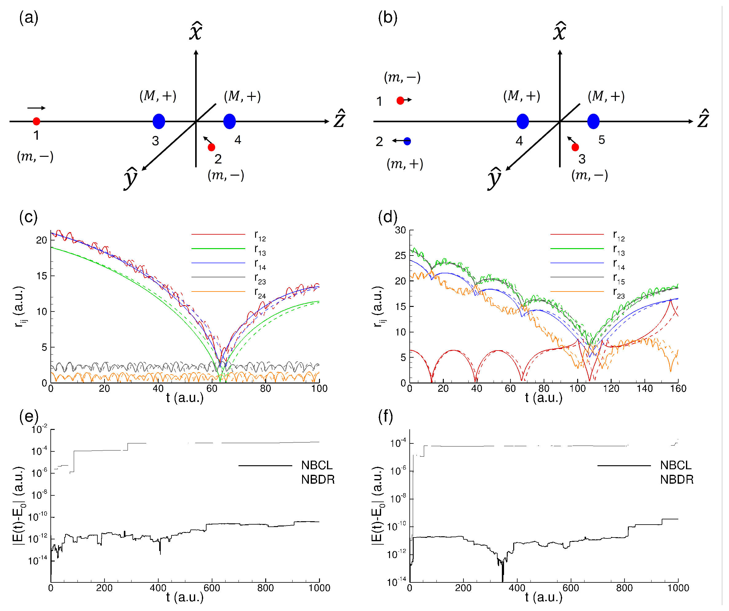
In this section, we provide sample calculations for the case of and 5 body systems. To investigate the accuracy and advantage of the regularized method, we also compute the trajectories by directly integrating the Hamilton’s equations fom Eq. (1) which fail when two or more particles have close encounters. For this purpose, we also provide a direct integrator program nbody-direct.f90 which does not employ any regularization. In Figure 1 we show the example calculations for the cases where we have and 3 charged particles. They may as well represent the collisions between an electron and a proton, and a collision between a positron and a hydrogen atom, respectively. Similarly, in Figure 2 we show the examples cases with and 5 bodies. The error in energy is analyzed in both Figure 1 and Figure 2 and it is clear that our method significantly reduces such an error compared to direct integration.
5. Conclusions and Outlook
We have presented a global regularization scheme for the Coulomb N-body problem that combines pairwise Kustaanheimo–Stiefel (KS) coordinates transformation followed by a time transformation. The method removes close-encounter singularities globally without recourse to case-by-case treatments and advances the dynamics. At the end of the trajectory run, the program returns the laboratory coordinates for analysis. Our Fortran implementation (nbodycl) follows the derivation presented in the paper verbatim.
Presented results on the test cases with and 5 bodies demonstrate the smooth behavior of the trajectories through near-collisions and tight control of the total energy. The optional electric-field coupling enables laser-driven regularized Coulomb dynamics within the dipole-approximation. This makes the nbodycl program directly applicable to problems in AMO physics such as laser-assisted electron–ion scattering and positron/positronium interactions.
Author Contributions
Conceptualization: H.B.A., I.I.F.; methodology: H.B.A., I.I.F.; software: H.B.A., M.K.M.; validation: H.B.A., M.K.M.; formal analysis: H.B.A., M.K.M.; investigation: H.B.A., I.I.F.; resources: H.B.A., I.I.F.; data curation: H.B.A., M.K.M.; original draft preparation: H.B.A., M.K.M.; review and editing: H.B.A., M.K.M., I.I.F.; visualization: H.B.A., M.K.M.; supervision: H.B.A.,and I.I.F.; project administration, H.B.A., I.I.F.; funding acquisition: H.B.A., I.I.F. All authors have read and agreed to the published version of the manuscript.
Funding
The work of M.K.M., and I.I.F was supported by the NSF under grant Nos. PHY-1803744 and PHY-2309261.
Acknowledgments
H. B. A. acknowledges the PHY-230160 grant from the Advanced Cyberinfrastructure Coordination Ecosystem: Services & Support (ACCESS) program, which is supported by NSF Grants No. 2138259, No. 2138286, No. 2138307, No.2137603, and No. 2138296
Conflicts of Interest
The authors declare no conflict of interest. The funders had no role in the design of the study; in the collection, analyses, or interpretation of data; in the writing of the manuscript, or in the decision to publish the results.The source code of the programs are available at Zenodo repository: https://doi.org/10.5281/zenodo.17804482.
Abbreviations
The following abbreviations are used in this manuscript:
| KS | Kustaanheimo-Steifel |
References
- Fabrikant, I.I.; Ambalampitiya, H.B. Laser-assisted radiative recombination in a cold hydrogen plasma. Journal of Physics B: Atomic, Molecular and Optical Physics 2024, 57, 195201. [CrossRef]
- Fabrikant, I.I.; Ambalampitiya, H.B.; Schneider, I.F. Semiclassical theory of laser-assisted dissociative recombination. Phys. Rev. A 2021, 103, 053115. [CrossRef]
- Fabrikant, I.I.; Ambalampitiya, H.B. Semiclassical theory of laser-assisted radiative recombination. Phys. Rev. A 2020, 101, 053401. [CrossRef]
- Ambalampitiya, H.B.; Stallbaumer, J.; Fabrikant, I.I. Laser-assisted charge transfer in positronium collisions with protons and antiprotons. Phys. Rev. A 2022, 105, 043111. [CrossRef]
- Ambalampitiya, H.B.; Fabrikant, I.I. Classical theory of laser-assisted spontaneous bremsstrahlung. Phys. Rev. A 2019, 99, 063404. [CrossRef]
- Price, H.; Lazarou, C.; Emmanouilidou, A. Toolkit for semiclassical computations for strongly driven molecules: Frustrated ionization of H2 driven by elliptical laser fields. Phys. Rev. A 2014, 90, 053419. [CrossRef]
- Peters, M.B.; Katsoulis, G.P.; Emmanouilidou, A. General model and toolkit for the ionization of three or more electrons in strongly driven atoms using an effective Coulomb potential for the interaction between bound electrons. Phys. Rev. A 2022, 105, 043102. [CrossRef]
- Katsoulis, G.P.; Peters, M.; Emmanouilidou, A. General model and toolkit for the ionization of three or more electrons in strongly driven molecules using an effective Coulomb potential for the interaction between bound electrons. Physical Review A 2024, 109, 033106.
- Aarseth, S.J. Gravitational N-Body Simulations: Tools and Algorithms; Cambridge Monographs on Mathematical Physics, Cambridge University Press, 2003.
- Szebehely, V. Theory of Orbits: The Restricted Problem of Three Bodies; Academic Press: New York, 1967. [CrossRef]
- Heggie, D.C. A global regularisation of the gravitationalN-body problem. Celestial mechanics 1974, 10, 217–241. [CrossRef]
- Mikkola, S. A practical and regular formulation of the N-body equations. Monthly Notices of the Royal Astronomical Society 1985, 215, 171–177, [https://academic.oup.com/mnras/article-pdf/215/2/171/3032631/mnras215-0171.pdf]. [CrossRef]
- Kustaanheimo, P.; Stiefel, E. Perturbation theory of Kepler motion based on spinor regularization. J. Reine Angew. Math. 1965, 218, 204–219.
- Yoshida, H. A new derivation of the Kustaanheimo-Stiefel variables. Celestial mechanics 1982, 28, 239–242. [CrossRef]
- Zare, K.; Szebehely, V. Time Transformations in the Extended Phase-Space. Celestial Mechanics 1975, 11, 469–482. [CrossRef]
- Press, W.H.; Teukolsky, S.A.; Vetterling, W.T.; Flannery, B.P. Numerical recipes in FORTRAN (2nd ed.): the art of scientific computing; Cambridge University Press: USA, 1992.
Figure 1.
Example calculations of trajectories for 2 (left column) and 3 (right column) bodies. Panels (a) and (b) show the initial configurations of the particles which are labeled as shown. The light particles have the same mass and the sign of their unit charges are given in the bracket. The heavier particle with mass is placed at the origin of the coordinates. The arrow indicates the initial direction of the particle’s momentum which is chosen arbitrarily. In Panels (c) and (d), the relative distances between the particle pairs are shown as function of time. The solid lines are the regularized trajectories obtained from the nbcl program, and the dashed lines are the corresponding results from direct integration using the nbody-direct program. In Panels (e) and (f), we show the difference between the starting energy and the run time energy of all the particles. This error in energy is significantly lower in the nbodycl (denoted by NBCL) calculations compared to those from nbody-direct (denoted ny NBDR).
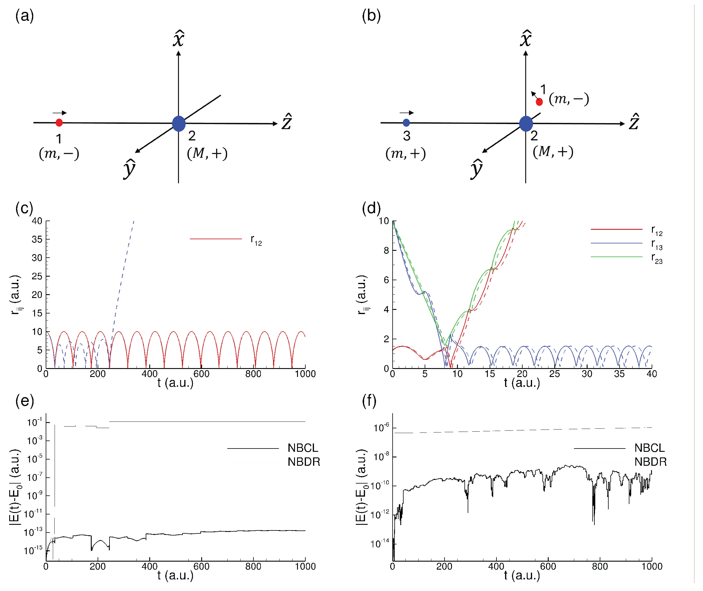
Figure 2.
Example calculations of trajectories for 4 (left column) and 5 (right column) bodies. Panels (a) and (b) show the initial configurations of the particles which are labeled as shown. All other details are as same as in Figure 1. In Panels (c) and (d), the relative distances between the particle pairs are shown as function of time. The solid lines are the regularized trajectories obtained from the nbodycl program, and the dashed lines are the corresponding results from direct integration using the nbody-direct program. In Panels (e) and (f), we show the difference between the starting energy and the run time energy of all the particles similar to Figure 1. Note that for the clarity of the figure, not all relative-separations are shown.
Disclaimer/Publisher’s Note: The statements, opinions and data contained in all publications are solely those of the individual author(s) and contributor(s) and not of MDPI and/or the editor(s). MDPI and/or the editor(s) disclaim responsibility for any injury to people or property resulting from any ideas, methods, instructions or products referred to in the content. |
© 2025 by the authors. Licensee MDPI, Basel, Switzerland. This article is an open access article distributed under the terms and conditions of the Creative Commons Attribution (CC BY) license (http://creativecommons.org/licenses/by/4.0/).
Copyright: This open access article is published under a Creative Commons CC BY 4.0 license, which permit the free download, distribution, and reuse, provided that the author and preprint are cited in any reuse.


