On the Nature of Gravitation and Geometric Drift of Spacetime

1. Introduction

An examination of the 1915–1916 formulation of General Relativity reveals that A. Einstein adopted the equivalence principle as a fundamental structural principle and was significantly influenced by the ideas of Ernst Mach. Within this framework, inertia was rendered a locally geometric property, and a local indistinguishability between accelerated frames and gravitational effects was established. Nevertheless, as the theory matured, the emergence of vacuum solutions and matter-free yet geometrically nontrivial spacetime structures demonstrated that General Relativity does not fully realize the Machian expectation that inertia be entirely determined by the global matter content of the universe.

Modern approaches to gravitation treat spacetime as a dynamical field that interacts with matter while remaining ontologically independent. In this perspective, gravity is identified as a manifestation of geometric structure, and the mere existence of spacetime is regarded as sufficient for a physical description. In contrast, the present work emphasizes that it is not only the existence of spacetime, but rather its inertial (kinematic) state, that plays a physically decisive role.

While the equivalence principle asserts the local indistinguishability of gravitational effects and accelerated reference frames, Mach’s principle posits that the inertial state of a body is determined by the total distribution of matter in the universe. Within the framework considered here, the determination of gravitation is not attributed solely to the matter content, but is shown to be intrinsically related to the inertial structure of the spacetime manifold itself.

In both General Relativity and its teleparallel equivalent formulation, gravitation is inherently described as a geometric phenomenon. The approach adopted in this study goes beyond accounting for the inertial properties of matter alone and demonstrates that gravitation may be interpreted as an effect arising from the inertial structure of spacetime. Although this difference may appear as a subtle modification at first glance, it leads to significant consequences for the conceptual framework underlying the geometric nature of gravitation.

An inertial observer experiences no force within their own reference frame, whereas an accelerated observer encounters effective force terms. The origin of these forces lies in the mismatch between the observer’s motion and the inertial structure of the spacetime geometry in which they are embedded. Cosmological observations, particularly those associated with the expansion of the universe, further indicate that inertial reference frames cannot be globally defined on a kinematically non-inertial background.

Within this context, inertial mismatch between an observer frame and the spacetime manifold may arise through two distinct mechanisms. In the first case, the mismatch results from the observer’s genuine accelerated motion relative to the manifold. In the second case, the observer is defined to possess fixed spatial coordinates in the chosen coordinate system; however, this condition cannot be reduced to a mere coordinate choice, since the observer’s worldline does not coincide with the natural congruence that defines the inertial structure of spacetime. Consequently, the effective force terms observed in this case are not coordinate artifacts, but are of genuine geometric origin. Although inertial mismatch is present in both scenarios, in the latter case the resulting effects appear to the observer as if they were intrinsic properties, corresponding precisely to the geometric origin of gravitation.

Before moving on to the next section, it would be necessary to briefly discuss the current state of modern gravity research. According to Riemannian approach existence of matter causes non-vanishing Riemann tensor components that may be transferred to Ricci Tensor and Scalar. On the other hand, an opposing view was again considered by Einstein such that Riemann tensor and therefore curvature of spacetime could still be kept zero without violating field equations. This latter theory is usually called as Teleparallel Gravity (TG) or Teleparallel Equivalent of General Relativity (TEGR) [1]. Even though GR and TEGR were (and still are) strong theories that are able to explain most of the cosmological phenomena, still remain some unsolved problems in physics awaiting explanation [2,3,4]. This has led scientists to search for alternative theories of gravity. Some of the studies questionize the source of the field equations while the others focus on geometrical point of view. The latter is divided into two parts: they either modify the classical curvature-centered approach, $f\left(R\right)$ theories [5,6,7], or propose studies based on modified torsion, namely $f\left(T\right)$ theories [8,9,10]. Felice et al. and Cai et al. give extensive reviews on these theories [7,8]. Carroll et al. address cosmic speed-up through modifications to the gravitational action of general relativity [5], similar to the approach of Bengochea and Ferraro [10], although the former involves $f\left(R\right)$ gravity, while the latter is based on $f\left(T\right)$. Krššák and Saridakis show that the same field equations could be obtained by the right spin connection choice for any observer. This study plays a fundamental role on good / bad tetrad discussion on teleparallel gravity [9]. The similarities and differences of the geometric background and dynamics underlying the current approach with the aforementioned studies will be presented in the following sections. The next section will then continue with interpretational remarks.

2. Interpretational Remarks

• This work is formulated within the framework of teleparallel geometry, where the spacetime connection satisfies

  $${R^a}_b\left(\omega \right)=0,$$

  (1)

  implying a Weitzenböck spacetime connection.
• In teleparallel geometries, torsion is not restricted to rotational contributions alone; rather, it encodes more general kinematic components, including shear, shift, expansion, and distortion. In the present work, this distinction plays a fundamental role in achieving a correct understanding of the geometric origin of gravitation.
• The torsion considered in this study is a physical geometric quantity and cannot be eliminated by coordinate transformations. Nevertheless, when described from accelerated (non-inertial) reference frames relative to inertial ones, coordinate-induced spurious torsional components may appear; however, such inertial contributions can be removed by an appropriate choice of the spin connection ${{\omega }^a}_b$. This necessitates a careful distinction between genuine physical torsion and frame-dependent apparent contributions [9].

• Within the tetrad formalism, an observer may in principle adopt infinitely many inequivalent tetrad choices. In the present work, this freedom is restricted by imposing the following conditions:

1.

Each observer employs a tetrad adapted to their own dynamical state, such that the tetrad choice reflects whether the observer is inertial or accelerated.

$$e^a\to {{\Lambda }^a}_b{e}^b,\omega \to \Lambda \omega {\Lambda }^{-1}+\Lambda d{\Lambda }^{-1},$$

(2)

2.

Physical torsion is defined as the torsion purified of inertial contributions by an appropriate choice of the spin connection. For inertial observers, this choice of tetrad remains compatible with the Weitzenböck connection, and the Fermi–Walker transport condition can be satisfied globally within the Weitzenböck gauge. In contrast, for accelerated observers this compatibility is generically broken: the Fermi–Walker condition cannot be maintained simultaneously with the Weitzenböck gauge. As a consequence, the spin connection becomes explicitly non-vanishing and contributes to the torsion tensor,

$$T^a=d{e}^a+{{\omega }^a}_b\wedge e^b,$$

(3)

leading to observer-dependent torsional effects in addition to pseudo-torsional contributions of inertial origin.

3.

All physical quantities are defined operationally by projection onto the observer’s tetrad,

$$A_{\left(a\right)}={e_{\left(a\right)}}^{\mu }{A}_{\mu }.$$

(4)

while fundamental geometric scalars remain observer-independent.

3. Geometric Framework

Teleparallel gravity was introduced to describe gravitation not as spacetime curvature, but as torsion allowing gravitational effects to be cleanly separated from inertial contributions and treated as a genuine force. In this concept, tetrads are the main mathematical objects and in the following subsection, the tetrad formalism that will be utilized throughout the study is presented.

3.1. Tetrad Formalism

The tetrad (or vierbein) formalism expresses the spacetime metric in terms of a local Lorentz frame. A tetrad field ${e^a}_{\mu }$ relates the coordinate metric $g_{\mu \nu }$ to the Minkowski metric ${\eta }_{ab}$ via

$$g_{\mu \nu }={e^a}_{\mu }{e^b}_{\nu }{\eta }_{ab}.$$

(5)

Here,

• Greek indices $(\mu ,\nu ,\dots )$ refer to coordinate frame,
• Latin indices $(a,b,\dots )$ refer to local Lorentz-frame.

Crucially, the tetrad formalism separates the metric structure (encoded in the tetrad itself) from the affine or spin connection, which can be chosen independently. This freedom allows the same tetrad to support different geometrical interpretations depending on the chosen connection.

In flat spacetime, the tetrad one-forms that correspond to each column of ${e^a}_{\mu }$ may be chosen as

$$e^0=cdt,e^i=d{x}^i.$$

(6)

The first column $e^0$ denotes the time-like direction, or in other words time part of the tetrad. The rest represent the local spatial directions in the local Lorentz frame. For example, in FLRW-type spacetimes, cosmological expansion is instead encoded in the spatial tetrad components through a time-dependent scale factor,

$$e^0=cdt,e^i=a\left(t\right)d{x}^i.$$

(7)

A dual basis exists for every tetrad such that

$$\begin{array}{c}{e_a}^{\mu }={\eta }_{ab}{g}^{\nu \mu }{e^b}_{\nu }\\ {e^b}_{\nu }{e_a}^{\nu }={\delta }_a^b.\end{array}$$

(8)

Unlike its dual, ${e_a}^{\mu }$ enables the transformation from local to general components. It indicates the observer’s velocity and orientation.

Within the revised Machian framework adopted in this work, it is argued that the route toward the equivalence principle is not, in general, fully compatible with the inertial structure of the spacetime manifold. If spacetime admits a preferred kinematical structure and an associated natural inertial congruence, then the physical interpretation of observers with fixed spatial coordinates,

$$x^i=\mathrm{const},$$

(9)

must be carefully reexamined. In particular, it becomes necessary to question whether such observers remain at the same physical spatial location as time evolves, or whether their worldlines generically deviate from the manifold’s natural inertial drift.

3.2. Geometric and Ontological Interpretation of the Drift Vector

Within the framework considered in this work, spacetime defines a preferred observer congruence $u^{\mu }$ determined by the tetrad structure and the associated drift field. In the present framework, the condition

$$u^{\mu }={e_0}^{\mu }$$

(10)

means that the observer moves along the natural geometric drift congruence defined by the tetrad. In this case, no kinematical mismatch arises and the effective gravitational force vanishes. This congruence represents the natural inertial motion that is compatible with the kinematical structure of the manifold.

An observer defined by Eq. (9) generally does not follow this congruence. Instead, the corresponding worldline deviates from the natural drift of spacetime. This deviation is fully encoded by the drift vector $W^i$, which precisely measures the mismatch between the observer’s worldline and the inertial congruence of the manifold.

In this perspective, the physical content of both gravitational and inertial effects is not interpreted as a direct force exerted by spacetime on matter. Rather, these effects emerge from the kinematical mismatch between the observer’s state of motion and the intrinsic inertial structure of spacetime. Within this viewpoint, observers whose motion is not aligned with the natural geometric congruence experience the effective consequences of this kinematical mismatch as inertial or gravitational effects.

The geometric content of gravitation thus arises as a kinematical phenomenon associated with the relative separation between the dynamical evolution of spacetime and the motion of observers embedded within it.

In this geometric framework, the drift vector $W^i$ naturally emerges as the quantity that characterizes the observer-dependent decomposition of spacetime’s kinematical structure. Since the tetrad formalism provides a transparent and observer-adapted description of this decomposition, it offers a natural and well-suited language for the analysis of gravitational structures within teleparallel geometry.

3.2.1. Tetrad Structure and Good Tetrad Conditions

In general, the tetrad field is written in its most general form as

$$e^0={e^0}_0(t,x)dt+{e^0}_i(t,x)d{x}^i,$$

(11)

$$e^i={e^i}_0(t,x)dt+{e^i}_j(t,x)d{x}^j.$$

(12)

Here, the tetrad is not chosen in an ad hoc manner, but is restricted to a well-defined subclass of the general $3+1$ decomposition,

$$e^0=Ndt,$$

(13)

$$e^i={E^i}_j(d{x}^j+N^{j}dt).$$

(14)

Each observer is required to employ a tetrad adapted to their own dynamical state; accordingly, the tetrad choice is made so as to reflect whether the observer is inertial or accelerated. Under this requirement, the lapse function is fixed to a constant value, $N=c$, and the temporal tetrad component reduces to

$$e^0=cdt.$$

(15)

When a geometric drfit field is defined for the universe on large scales, the form of the tetrad is strongly constrained by cosmological symmetries. Isotropy forbids any preferred spatial direction in the spatial tetrad components, while homogeneity excludes any explicit dependence on spatial position.

Examining the spatial tetrad structure

$$e^i={E^i}_j(d{x}^j+N^{j}dt),$$

(16)

one finds that the internal spatial geometry encoded in ${E^i}_j$ must, by isotropy, be proportional to the Kronecker delta,

$${E^i}_j\propto {{\delta }^i}_j.$$

(17)

Homogeneity further requires that the proportionality factor depend on time only. Consistency with FLRW symmetry therefore uniquely fixes

$${E^i}_j=a\left(t\right){{\delta }^i}_j.$$

(18)

In the presence of cosmic expansion, the physical spatial location associated with matter is not preserved relative to fixed coordinate labels. Instead, the manifold itself induces a kinematical transport of matter through the expanding geometry. The relative shift between the temporal direction and the spatial tetrad is encoded in the vector $N^j$.

This component acts as the natural carrier of the cosmological drift within the tetrad structure and is therefore identified with the drift field. Accordingly, written as

$$N^j={\displaystyle \frac{W^i}{a\left(t\right)}}.$$

(19)

A vector field of the form $W^i=\mathrm{const}$ is not admissible, since it would select a preferred spatial direction and thereby violate isotropy. Such a structure is not invariant under $\mathrm{SO}\left(3\right)$ and consequently violates cosmological isotropy. For this reason, constant nonzero drift vectors are excluded. Moreover, allowing the coefficients of $W^i$ to depend arbitrarily on spatial position would generically jeopardize homogeneity. For this reason, the most general homogeneous configuration requires $W^i$ to be at most linear in the spatial coordinates, (see Appendix I)

$$W_{\mathrm{global}}^i=b\left(t\right)x^i.$$

(20)

This form is covariant under spatial rotations and does not define any preferred direction. Although the global drift field appears at first sight to single out a preferred origin, this dependence is purely coordinate-based and has no physical significance. This structure is the tetrad-level analogue of the Hubble flow $v^i=H{x}^i$ in standard FLRW cosmology where H is the Hubble constant.

The physical observables depend only on the derivatives of $W^i$, and the resulting torsion tensor is spatially homogeneous and translation invariant. Consequently, the drift field does not introduce a preferred center and is fully consistent with cosmological homogeneity and the Copernican principle.

3.2.2. Lorentz Signature and Causality

At this point, it is essential to emphasize that the drift field $W^i$ is constrained not only by symmetry requirements, but also by the preservation of Lorentz signature and causality.

An additional condition therefore comes into play. In close analogy with Einstein–Æther–type constructions, the requirement of causal consistency demands that the metric induced by the tetrad retain a Lorentzian signature. Writing the metric in ADM form,

$$d{s}^2=-N^{2}d{t}^2+{\gamma }_{ij}\left(d{x}^i+N^{i}dt\right)\left(d{x}^j+N^{j}dt\right),$$

(21)

that can be rewritten explicitly as below for the specific choice of lapse $N=c$, shift $N^i=a{W}^i$ and spatial metric ${\gamma }_{ij}=a^2{\delta }_{ij}$:

$$d{s}^2=-(c^2-W^2)d{t}^2+2a{W}_{i}d{x}^{i}dt+a^2{\delta }_{ij}d{x}^{i}d{x}^j,W^2:={\delta }_{ij}{W}^i{W}^j,$$

(22)

one immediately finds that preservation of the Lorentzian signature $(-1,1,1,1)$ requires

$$c^2-W^2>0,$$

(23)

or equivalently $c^2>W^2$. Under this condition, causality is preserved and the model remains free of superluminal pathologies.

Taken together, these considerations imply that the most general form of the tetrad compatible with cosmological symmetries, Lorentz signature, and causality is

$$e^0=cdt,e^i=a\left(t\right)d{x}^i+W_i(t,\mathbf{x})dt.$$

(24)

Thus, the spatial tetrad components may contain only a time–dependent scale factor and a single flow drift term encoding temporal–spatial mixing. The tetrad choice is therefore not arbitrary, but arises as the natural consequence of imposing cosmological symmetries on the most general observer-adapted tetrad.

In this framework, the drift field $W^i$ is a physical quantity. The conditions under which it represents a genuine geometric structure, rather than a coordinate or inertial artifact, will be examined in detail in the following discussion.

3.3. On the Physical Nature of $W^i$

At this stage, the central question is the following: is $W^i$ a spurious effect arising from a particular choice of observer, or is it a physical geometric quantity originating from the kinematical structure of the manifold, which cannot be eliminated by a change of observer?

In order to address this question, let us consider the structure of the manifold in its simplest form:

1.

The manifold is isotropic, admitting no preferred spatial direction.

2.

The manifold is homogeneous, admitting no dependence on a distinguished spatial point.

Furthermore, under a change of observer, the vector $W^i$ must remain invariant. Consequently, $W^i$ cannot originate from observer acceleration and must not be interpreted as an acceleration-induced quantity.

Under these assumptions, the only consistent way to understand the origin of the geometric drift vector is to analyze it within the kinematical decomposition of an observer congruence defined independently of the dynamical field equations.

3.3.1. Physical Structure of the $W^i$ Field

In teleparallel geometry, since the physical field strength is given by torsion, a transformation can be regarded as a gauge transformation only if it leaves the torsion unchanged. Any transformation that modifies torsion changes the physical content and therefore is not a gauge transformation.

Under the drift-adapted tetrad employed in this work as given in Eq. (24) we may consider the shift

$$W^i⟶W^i+{\partial }_t{\Lambda }^i.$$

(25)

In the Weitzenböck gauge $({{\omega }^a}_b=0)$, it is straightforward to verify (see Appendix II.A) that torsion changes,

$$\delta T^i\ne 0.$$

(26)

More importantly, this result is not restricted to the Weitzenböck gauge. In the fully covariant teleparallel formulation, which we will analyze for accelerated observers, the above shift does not correspond to a local Lorentz transformation. Therefore, it cannot be compensated by a pure-gauge change in the spin connection, and in general (see Appendix II.B),

$$\delta T^a\ne 0.$$

(27)

Consequently, the field $W^i$ modifies the torsional field strength and is not a gauge degree of freedom in teleparallel geometry. It should therefore be interpreted as a physical geometric drift field associated with the inertial structure of spacetime.

Another concern would be on the non–removability of $W^i$ by diffeomorphisms. The physically relevant quantity in the geometric drift velocity (GDV) framework is the scalar projection

$$\mathcal{S}\equiv T_{\mu }{u}^{\mu }.$$

(28)

This object is a true spacetime scalar under diffeomorphisms. Therefore, under any coordinate transformation,

$${\mathcal{S}}^{\prime }\left(x^{\prime }\right)=\mathcal{S}\left(x\right).$$

(29)

Suppose that a diffeomorphism existed that removes the drift field, $W^i\to 0$. The torsion tensor would then change structurally, and the computed value of $T_{\mu }{u}^{\mu }$ would differ from its original value. This would contradict diffeomorphism invariance.

Hence, no diffeomorphism can eliminate $W^i$ while preserving the scalar $T_{\mu }{u}^{\mu }$. The drift field is therefore not a coordinate artifact but a physically meaningful geometric structure. The drift vector is a physical component of the observer-adapted tetrad. It contributes directly to the torsion tensor and therefore cannot be removed by local Lorentz gauge transformations or inertial spin-connection redefinitions.

3.3.2. Metric and kinematical decomposition

Let $u^{\mu }$ denote a timelike observer congruence satisfying the normalization condition (Please see Appendix III.A to III.C)

$$u^{\mu }{u}_{\mu }=-1,$$

(30)

The spatial projection tensor is defined by

$$h_{\mu \nu }:=g_{\mu \nu }+u_{\mu }{u}_{\nu }.$$

(31)

The covariant derivative of the congruence can then be decomposed kinematically as [8,11]

$${\nabla }_{\nu }{u}_{\mu }=-a_{\mu }{u}_{\nu }+{\displaystyle \frac{1}{3}}\theta h_{\mu \nu }+{\sigma }_{\mu \nu }+{\tilde{\omega }}_{\mu \nu },$$

(32)

where $a^{\mu }:=u^{\nu }{\nabla }_{\nu }{u}^{\mu }$ is the four–acceleration of the congruence, $\theta :={\nabla }_{\mu }{u}^{\mu }$ is the expansion scalar,

$${\sigma }_{\mu \nu }:={h_{\mu }}^{\alpha }{h_{\nu }}^{\beta }{\nabla }_{(\alpha }{u}_{\beta )}-{\displaystyle \frac{1}{3}}\theta h_{\mu \nu }$$

(33)

is the shear tensor, and

$${\tilde{\omega }}_{\mu \nu }:={h_{\mu }}^{\alpha }{h_{\nu }}^{\beta }{\nabla }_{[\alpha }{u}_{\beta ]}$$

(34)

is the vorticity tensor. In this case, each tensor will be examined in detail.

Acceleration contribution in the kinematical decomposition

The acceleration of an observer congruence is defined by

$$a^{\mu }:=u^{\nu }{\nabla }_{\nu }{u}^{\mu }.$$

(35)

For the tetrad employed in this work, the covariant components of the natural congruence are found to be (see Appendix III.B)

$$u_{\mu }=(-c,0,0,0).$$

(36)

In this decomposition, the lapse function takes the constant value $N=c$. By definition, $a_{\mu }={\displaystyle \frac{1}{N}}{D}_{\mu }N$, one therefore has

$$D_{\mu }(lnN)=D_{\mu }(lnc)=0,$$

(37)

which directly implies

$$a_{\mu }=0⟹a^{\mu }=0.$$

(38)

This result demonstrates that, for the natural congruence defined by the chosen tetrad, there is no contribution from acceleration in the kinematical decomposition.

Vorticity contribution to the kinematical decomposition

Vorticity characterizes the rotational properties of the observer congruence. In the teleparallel formalism, the simplest and most natural choice is

$$u^{\mu }:={e_0}^{\mu }.$$

(39)

Furthermore, since

$$u_{\mu }=(-c,0,0,0),$$

(40)

the observer congruence is hypersurface–orthogonal and irrotational. Consequently, the vorticity tensor ${\tilde{\omega }}_{\mu \nu }$ vanishes identically, (Please see Appendix III.D)

$${\tilde{\omega }}_{\mu \nu }=0.$$

(41)

Shear contribution to the kinematical decomposition

The shear tensor takes the form

$${\sigma }_{ij}={\displaystyle \frac{a}{c}}\left[{\displaystyle \frac{1}{3}}\left({\partial }_k{W}^k\right){\delta }_{ij}-{\displaystyle \frac{1}{2}}\left({\partial }_i{W}_j+{\partial }_j{W}_i\right)\right].$$

(42)

Since the choice $W_i=b\left(t\right)x_i$ is the only one compatible with spatial homogeneity, it follows immediately that (Please see Appendix III.E)

$${\sigma }_{ij}=0.$$

(43)

Moreover, because the observer congruence undergoes isotropic expansion, the full shear tensor ${\sigma }_{\mu \nu }$ vanishes identically.

Expansion contribution to the kinematical decomposition

The expansion of the observer congruence is defined as

$$\theta :={\nabla }_{\mu }{u}^{\mu }.$$

(44)

For the tetrad considered in this work, this quantity is obtained explicitly as

$$\theta ={\displaystyle \frac{1}{ac}}\left(3\dot{a}-{\partial }_i{W}^i\right).$$

(45)

In particular, for the case $W^i=0$, one finds (Please see Appendix III.F)

$$\theta ={\displaystyle \frac{3\dot{a}}{ac}},$$

(46)

which coincides with the standard cosmological expansion of comoving observers in FLRW spacetime.

Taking all contributions into account, the only nonvanishing term in the kinematical decomposition is the expansion. Therefore, we have

$${\nabla }_{\nu }{u}_{\mu }={\displaystyle \frac{1}{3}}\theta h_{\mu \nu }.$$

(47)

The fact that an expanding manifold gives rise exclusively to an isotropic expansion term, while acceleration, vorticity, and shear vanish identically due to homogeneity, isotropy, and observer independence is of central importance for the internal consistency of the theory.

Reducing the kinematical decomposition to pure isotropic expansion demonstrates that this expansion originates from the inertial structure of spacetime itself. In teleparallel geometry, where inertial structure is encoded in torsion rather than curvature, a discussion of the physical content of expansion therefore necessarily requires passing from the metric description to an analysis in terms of torsion.

3.4. Metric

The resulting metric takes the form

$$g_{\mu \nu }=\left(\begin{array}{cccc}-(c^2-|W{|}^2)& a{W}_1& a{W}_2& a{W}_3\\ a{W}_1& a^2& 0& 0\\ a{W}_2& 0& a^2& 0\\ a{W}_3& 0& 0& a^2\end{array}\right),$$

(48)

where the time–space components induced by the chosen tetrad structure are nonvanishing,

$$g_{0i}=a\left(t\right)W_i.$$

(49)

This shows that the temporal and spatial directions do not fully decouple at the metric level, and that the spatial frames are transported along time with a certain drift. The factor $a\left(t\right)$ sets the cosmological scaling of this effect, while the field $W_i$ encodes the spatial structure of the drift.

In the present framework, the drift field $W^i$ characterizes the transport (dragging) of spatial frames along the temporal direction. The nonvanishing components $g_{0i}=a\left(t\right)W_i$ encode this effect at the metric level, indicating that spatial frames are continuously GDVected in time rather than remaining orthogonal to it. In this sense, drift represents the geometric dragging of spatial directions by the temporal flow of spacetime.

Although these terms are formally reminiscent of the shift vector in the ADM decomposition, the contribution $a{W}_i$ that appears here cannot be interpreted purely as a consequence of a coordinate choice. Indeed, $W_i$ is directly tied to the temporal structure of the tetrad and therefore carries kinematical content: it specifies how the spatial frames are transported along the time direction.

Consequently, the question of whether the mixing observed at the metric level represents a merely inertial effect or a genuine feature of spacetime geometry can be clarified in a sharp way only by passing to the teleparallel description, where the relevant notion is torsion.

3.5. Lorentz Covariance of Torsion

In the discussion of the physical nature and necessity of the field $W_i$, the concept of torsion—one of the fundamental geometric objects of teleparallel geometry—plays a central role. In this section, we systematically analyze the geometric definition of torsion and its manifestation for different classes of observers. In particular, observers in Minkowski spacetime, static observers (i.e. observers with fixed spatial coordinates), freely falling observers, and accelerated observers will be treated separately. Special emphasis is placed on the distinction between spurious (inertial) torsion contributions arising in accelerated frames and genuine geometric torsion.

Within this framework, the question of whether the origin of the field $W_i$ can be traced to spurious torsion effects or to the true geometric torsion of spacetime will be answered in a precise and unambiguous manner.

The tetrad structure adopted throughout this work is given by Eq. (24) and the general definition of torsion tensor is given by Eq. (3).

For non-accelerated observers, guided by the Fermi–Walker conditions introduced earlier, one may consistently employ the Weitzenböck connection. However, once accelerated observers are considered, contributions from the spin connection necessarily arise, giving rise to spurious torsion effects. In the Weitzenböck gauge,

$${{\omega }^a}_b=0,T^a:=d{e}^a.$$

(50)

Carrying out the intermediate steps explicitly (see Appendix IV.A), one finds

$$T^i=d{e}^i=\left(\dot{a}{{\delta }^i}_j-{\partial }_j{W}_i\right)dt\wedge d{x}^j.$$

(51)

Under the chosen tetrad structure, the computation of torsion reveals that only the components corresponding to time–space mixing are non-vanishing. The resulting component,

$${T^i}_{0j}={\displaystyle \frac{1}{a}}\left(\dot{a}{{\delta }^i}_j-{\partial }_j{W}_i\right),$$

(52)

measures the mismatch between the temporal evolution of space and the spatial structure of the selected drift field.

Torsion thus emerges as the direct geometric expression of the difference between how space expands and how matter or observers are transported within that expansion. Since acceleration, rotation, and shear vanish identically in the present setting, no other kinematical structure remains that could encode this mismatch. Consequently, the entire physical content of torsion is necessarily concentrated in the component ${T^i}_{0j}$.

This result demonstrates explicitly that the field $W_i$ is not a spurious coordinate artifact, but a physical geometric field associated with the inertial structure of spacetime.

The reason why this component cannot, in general, be set to zero is that the term ${\partial }_j{W}_i$ contains a genuine geometric contribution tied to the global kinematical structure of spacetime, which cannot be eliminated by a local Lorentz transformation or by a suitable choice of spin connection.

Nevertheless, the question of whether $W_i$ originates from spurious torsion or from genuine geometric torsion must still be explicitly addressed. To this end, the definition and explicit computation of torsion for observers in free fall, observers at rest with respect to the ground, observers in empty space, and accelerated observers will be presented in detail, together with a clear account of the conventions and calculations required to separate inertial from geometric contributions.

3.5.1. Discussion on the Good Tetrad

In teleparallel geometries, infinitely many tetrad choices correspond to the same metric structure. This freedom arises because tetrads describe local observer frames rather than the spacetime geometry itself. However, not every tetrad choice correctly reflects the physical content of the torsion tensor.

In particular, within the pure tetrad formulation where the spin connection is set to zero, an inappropriate tetrad choice may lead to inertial contributions—associated with acceleration and rotation—being improperly encoded into the torsion tensor. In such cases, torsion does not represent purely gravitational effects, but also contains spurious inertial artifacts.

In the literature, tetrads that avoid this issue are referred to as good tetrads. A good tetrad is defined as one that, even when the spin connection is set to zero, does not generate torsion in Minkowski spacetime and contains only genuine geometric (gravitational) torsion components. Such tetrads prevent inertial effects from mixing with torsion and thereby ensure the consistency of the geometric interpretation.

The tetrad structure employed in the present work possesses this good tetrad property for inertial, freely falling, and Fermi–Walker transported observer frames. In these cases, it is consistent to set the spin connection to zero. In contrast, when accelerated observers are considered, the covariant teleparallel formulation is adopted and an appropriate curvature-free spin connection is introduced. This prevents inertial contributions from being incorrectly transferred into the torsion tensor.

Therefore, the use of a good tetrad in this work is not assumed universally, but is applied consistently depending on the physical class of observers. This approach guarantees that torsion is interpreted as an observer-independent quantity associated with the inertial and geometric structure of spacetime.

It is worth noting that this kinematical separation has a conceptual connection to discussions in the literature on nonlinear teleparallel generalizations. In particular, the Lorentz frame dependence issues encountered in $f\left(T\right)$-type theories can be understood as a dynamical manifestation of the failure to separate inertial contributions from genuine geometric torsion. As shown by M. Krššák and E. N. Saridakis, for any given form of $f\left(T\right)$, the field equations are satisfied by all tetrads related through a Lorentz transformation. In other words, within $f\left(T\right)$ gravity there is no intrinsic distinction between good and bad tetrads, provided that one does not impose a vanishing spin connection, namely the Weitzenböck gauge. Once this restriction is lifted and the appropriate inertial spin connection is properly taken into account, the theory does not exhibit frame dependence [9].

Although no $f\left(T\right)$-type generalization is considered in the present work and the action itself is not modified at that level, the approach adopted here sheds light on the more fundamental, kinematical origin of such problems.

3.5.2. Torsion for an Observer in Minkowski Spacetime

In flat spacetime (Minkowski spacetime), since there is no matter or energy-momentum distribution capable of disturbing inertial motion, no geometric flow or drift of spacetime can arise. Consequently, the field $W^i$ that characterizes the inertial structure of spacetime vanishes physically.

In this case, a standard tetrad choice defined in Cartesian coordinates may be adopted, as given by Eq. (6) which represents a family of observers that is nonrotating, nonaccelerated, and free of any shift. In Minkowski spacetime, for this tetrad choice,

$$T^a=d{e}^a.$$

(53)

However, for the chosen tetrad one has

$$d{e}^0=d\left(cdt\right)=0,d{e}^i=d\left(d{x}^i\right)=0,$$

(54)

and therefore all components of torsion collapse to zero:

$$T^a=0.$$

(55)

This result is consistent with the weak interpretation of Mach’s principle: in a spacetime devoid of matter and energy–momentum content, no geometric structure capable of defining inertia or spatial drift ($W^i$) can arise. Consequently, teleparallel torsion vanishes physically in vacuum.

However, an important distinction must be emphasized. Even in Minkowski spacetime, if one passes to an accelerated or rotating coordinate system while keeping the spin connection fixed at ${{\omega }^a}_b=0$, a mathematically nonvanishing torsion may be obtained. Such torsion does not belong to spacetime itself, but instead represents a spurious torsion originating from the noninertial motion of the observer.

Therefore, the result $T^a=0$ obtained in empty space defines the fundamental reference limit for the definition of physical torsion—and hence of the gravitational field—in teleparallel geometry. The field $W^i$ can acquire nonvanishing values only when spacetime is disturbed by matter-energy content.

3.5.3. Observer at Rest: Static Frame and the Separation of Geometric Torsion

An observer at rest is defined, within the chosen coordinate system, by the condition that their spatial position does not change with time, expressed as

$$u^i=0.$$

(56)

However, this static definition does not imply that the observer follows a physically inertial (geodesic) worldline. Within the teleparallel framework, the physical velocity measured by an observer in the tetrad frame is defined as

$$v^i:=a\left(t\right)u^i+W^i.$$

(57)

For an observer at rest, this immediately yields

$$v^i=W^i.$$

(58)

This expression shows that inertial observer corresponds to a relative motion with respect to the local drift structure of spacetime.

The central question at this point is whether the observer’s acceleration generates spurious (inertial) contributions to the torsion tensor. In general, in accelerated observer frames, inappropriate tetrad choices may introduce inertial terms into the torsion tensor. However, in the present work, the tetrad of the observer at rest is deliberately chosen to be compatible with Fermi–Walker transport. This choice allows kinematical effects associated with the observer’s proper acceleration to be separated through the connection structure rather than being absorbed into torsion.

As a result, only genuine torsion contributions appear in the torsion expression, and these contributions originate from the inertial structure and expansion of the manifold itself.

In teleparallel formalism, this situation is realized by employing the Weitzenböck connection under a proper (good) tetrad choice, allowing the spin connection to be taken as

$${{\omega }^a}_b=0.$$

(59)

This choice is not an arbitrary gauge fixing, but rather a geometric consistency condition ensuring that inertial effects associated with the observer do not contaminate the torsion tensor. In this way, the resulting torsion is free of observer acceleration and encodes only information about the geometric structure of spacetime.

Under these conditions, the relevant torsion component computed for the observer at rest is (Please see Appendix IV.B)

$${\left({T^i}_{0j}\right)}_{\mathrm{rest}}={\displaystyle \frac{1}{a}}\left[(\dot{a}-b){{\delta }^i}_j+{\partial }_j{W}_i^{\mathrm{adapt}}\right]\ne 0.$$

(60)

This result demonstrates that torsion is not a quantity tied to the observer’s acceleration; rather, acceleration determines only the dynamical interaction of the observer with the geometric structure.

This expression represents the superposition of two distinct geometric contributions. The first term encodes the mismatch between the temporal scaling of spacetime and the adaptation of the tetrad to this evolution, while the second term reflects the spatial gradient of the drift field $W^i$, that is, the differential variation of the local flow structure of spacetime.

This result again confirms that torsion is not dependent on the observer’s acceleration; acceleration affects only how the observer dynamically interacts with the geometric structure. In particular, the second term reveals that torsion is not a gauge quantity but a physical geometric magnitude.

At this stage, the ontological status of the field $W^i$ becomes clear. If $W^i$ were merely an inertial gauge artifact arising from the choice of an accelerated reference frame, then, according to the fundamental principles of covariant teleparallel theory, one could eliminate torsion entirely by an appropriate local Lorentz transformation accompanied by a nonvanishing spin connection.

However, as long as cross terms such as $g_{0i}$ persist at the metric level, the contribution of $W^i$ to torsion remains an inseparable geometric reality. For this reason, $W^i$ represents not a simple coordinate velocity in empty space, but a geometric drift structure determined by the matter–energy content of spacetime.

Consequently, the acceleration of an observer at rest is not the source of the observed torsion, but rather a result of the physical resistance to the geometric drift of spacetime.

3.5.4. Torsion for a Freely Falling Observer

A freely falling observer is defined by the condition that the physical velocity measured in the tetrad frame does not change with time,

$${\displaystyle \frac{d{v}^i}{dt}}=0.$$

(61)

In particular, under the condition $v^i=0$, this implies that the observer follows the local drift field of spacetime exactly, that is,

$$a\left(t\right)u^i=-W^i.$$

(62)

Physically, this corresponds to the ideal inertial situation in which the observer experiences no inertial forces and moves together with the geometric flow of spacetime. Nevertheless, when the relevant torsion component is computed (see Appendix IV.C), one finds

$${\left({T^i}_{0j}\right)}_{\mathrm{free}\mathrm{fall}}={\displaystyle \frac{1}{a}}\left[(\dot{a}-b){{\delta }^i}_j+{\partial }_j{W}_i^{\mathrm{adapt}}\right].$$

(63)

This expression is mathematically identical to the torsion component obtained for the observer at rest and is generally nonvanishing. Torsion is therefore not a quantity that depends on the dynamical state of the observer (accelerated or freely falling), but a covariant geometric object belonging to the inertial structure of spacetime.

In this sense, observers at rest and freely falling observers are in complete agreement regarding the value of the torsion field. The difference between them lies not in the value of torsion itself, but in the way this geometric structure affects their dynamics.

This covariance property also holds for accelerated observers; however, in that case the distinction between genuine and spurious torsion becomes essential. Genuine torsion is determined by the metric and spacetime geometry and cannot be eliminated by a suitable choice of spin connection. Spurious torsion, by contrast, represents inertial contributions that depend solely on the choice of frame and can be removed by an appropriate spin connection. This distinction will be analyzed in detail in the following subsection.

3.5.5. Accelerated Observers and the Covariant Transformation of Torsion

In accelerated observer frames, the physical content of torsion can be meaningfully analyzed only through the fully covariant definition that includes spin connection contributions. In teleparallel geometry, the torsion 2–form is defined by Eq. (3).

The behavior of this definition under local Lorentz transformations determines whether torsion represents a mere frame artifact or an observer–independent geometric quantity. In teleparallel formalism, spurious torsion is defined as a mathematical artifact that arises even in flat Minkowski spacetime when an inappropriate tetrad choice is combined with an incomplete or incorrect spin connection. Such contributions do not belong to the physical geometry of spacetime, but solely to the acceleration of the observer and the chosen frame. For this reason, the separation of inertial effects from physical torsion crucially depends on the correct choice of spin connection.

The tetrad field of an accelerated observer is obtained from a reference inertial tetrad $e^a$ via a spacetime–dependent local Lorentz transformation ${{\Lambda }^a}_b\left(x\right)$:

$$e^{\prime a}={{\Lambda }^a}_b\left(x\right)e^b.$$

(64)

In order to prevent the acceleration and rotation introduced by this transformation from contaminating the physical (gravitational) content of torsion, the spin connection must be chosen in a pure–gauge form that remains curvature-free,

$${{\omega }^{\prime a}}_b={{\Lambda }^a}_{c}d{{\left({\Lambda }^{-1}\right)}^c}_b,{R^a}_{bcd}=0.$$

(65)

This choice guarantees that all inertial effects are absorbed into the spin connection and that the torsion tensor represents only genuine geometric content.

Under these conditions, torsion transforms as a fully tensorial quantity,

$$T^{\prime a}=d{e}^{\prime a}+{{\omega }^{\prime a}}_b\wedge e^{\prime b}={{\Lambda }^a}_b{T}^b.$$

(66)

It has thus been shown that there is no ontological discrepancy in the status of torsion between accelerated, stationary, and freely falling observers. The “frame dependence” problem frequently discussed in the literature arises, in most cases, from imposing $\omega =0$ (pure tetrad) in accelerated frames, thereby incorrectly transferring inertial contributions into the torsion tensor.

In summary, accelerated and freely falling observers at the same spacetime point measure the same physical torsion; the difference between them lies only in how the tetrad components of this torsion are labeled under local Lorentz transformations. The invariance of the torsion derived from the drift field $W^i$ under such transformations demonstrates unambiguously that it is not a coordinate or frame artifact, but an objective geometric invariant determined by the matter-energy content of spacetime. This result clearly establishes torsion as a real geometric field that is independent of the observer. Different observers:

• live in the same torsion field,
• measure the same genuine torsion,
• but have different dynamical relations (acceleration, force) to this torsion.

There is therefore no disagreement between observers regarding torsion itself; differences arise only in the interpretation of acceleration and motion.

Up to this point, it has been demonstrated that the geometric drift field $W^i$ carries an observer–independent, physical torsion content that necessarily emerges through kinematical decomposition.

Given the curvature-free but torsionful nature of teleparallel geometry, particle motion is naturally described in terms of autoparallels associated with the teleparallel connection. When this motion is re-expressed with respect to the Levi–Civita connection, deviations from geodesic motion arise, which are entirely encoded in the contortion tensor measuring the difference between the two connections. The geometric and physical content of this tensor will be analyzed in detail in the following section.

4. From Kinematics to Dynamics

4.1. Contortion and Inertial Mismatch

In what follows, the geometric origin of the inertial mismatch emerging in free particle motion is clarified by expressing the difference between the teleparallel and Levi–Civita connections through the contortion tensor.

4.1.1. Difference Between Levi–Civita and Teleparallel Connections

A fundamental feature of teleparallel geometry is that spacetime is described by a connection that is free of curvature but possesses torsion. In contrast, the Levi–Civita connection is metric-compatible and torsion-free, representing the standard connection employed in General Relativity.

Although these two connections share the same metric structure, they define parallel transport and the notion of geodesics in fundamentally different ways. Consequently, it is necessary to explicitly identify and geometrically characterize the difference between the teleparallel and Levi-Civita connections.

4.1.2. Contortion Tensor

The difference between these two connections defined on the same metric manifold is encoded in the contortion tensor, which measures the deviation of the teleparallel connection from the Levi–Civita connection.

In this context, the relationship between the teleparallel connection ${{\Gamma }^{\rho }}_{\mu \nu }$, the Levi–Civita connection ${{\{}^{\rho }}_{\mu \nu }\}$, and the contortion tensor ${K^{\rho }}_{\mu \nu }$ is given by

$${{\Gamma }^{\rho }}_{\mu \nu }={{\{}^{\rho }}_{\mu \nu }\}+{K^{\rho }}_{\mu \nu }.$$

(67)

This expression makes it clear that the contortion tensor does not represent an independent geometric structure, but rather encodes the difference between a torsionful parallel transport rule and the torsion-free Levi–Civita geometry.

The contortion tensor is defined directly in terms of the torsion tensor and therefore carries information intrinsic to the kinematic structure of spacetime. In the present work, torsion encodes the mismatch between the natural inertial congruence of spacetime and the motion of a given observer or particle. Accordingly, the contortion tensor becomes the fundamental quantity that determines how this inertial deviation manifests itself within the Levi–Civita geometric framework.

The contortion tensor, together with the associated superpotential tensor, constitutes the basic geometric building blocks of the teleparallel Lagrangian structure. The contortion tensor is defined as

$${K_{\mu \nu }}^{\rho }=-{\displaystyle \frac{1}{2}}\left({T_{\mu \nu }}^{\rho }-{T_{\nu \mu }}^{\rho }-{T^{\rho }}_{\mu \nu }\right).$$

(68)

4.1.3. Components of the Contortion Tensor

For the tetrad structure employed in this work, the non-vanishing components of the contortion tensor are obtained as follows. (Please see Appendix V.A)

• The symmetric contortion component ${K^i}_{0j}$ encodes the mismatch between the inertial flow of spacetime and the motion of a particle. This mismatch is determined by the geometric drift field $W^i$ and represents the teleparallel geometric expression of inertial incompatibility.

$$\begin{array}{cc}\hfill {K^i}_{0j}& ={\displaystyle \frac{1}{2}}\left({T^j}_{i0}+{T^i}_{j0}\right),\hfill \end{array}$$

(69)

• This antisymmetric component represents the local rotational or vortical structure of spacetime. Within the framework considered here, this term corresponds to the rotational contributions of the flow field and vanishes at cosmological scales due to isotropy, while producing Coriolis-like effects in local systems.

$$\begin{array}{cc}\hfill {K^i}_{j0}& ={\displaystyle \frac{1}{2}}\left({T^j}_{i0}-{T^i}_{j0}\right),\hfill \end{array}$$

(70)

• The algebraic relation between the component ${K^0}_{ij}$ and ${K^i}_{0j}$ indicates that the mismatch between temporal and spatial components originates from the same geometric source.

$$\begin{array}{cc}\hfill {K^0}_{ij}& =-{K^i}_{0j},\hfill \end{array}$$

(71)

• In contrast, the vanishing of the purely spatial components ${K^i}_{jk}=0$ implies that space itself does not contain any intrinsic inertial distortion, shear, or rotation. All physical effects arise from the interplay between the temporal evolution of space and the underlying flow structure.

$$\begin{array}{cc}\hfill {K^i}_{jk}& =0.\hfill \end{array}$$

(72)

Taken together, these results demonstrate that the contortion tensor carries physical content exclusively through time–space mixing components.

The contortion tensor thus shows that $W^i$ is not merely a kinematic parameter, but a physical inertial field that modifies the geometric definition of free particle motion.

4.1.4. Role of Contortion in Free Particle Motion

In the teleparallel framework, the assumption of inertial motion is expressed by the vanishing of the proper acceleration defined with respect to the drift-adapted tetrad frame:

$${\displaystyle \frac{d{v}^i}{dt}}=0.$$

(73)

Here, $v^i$ denotes the physical velocity measured relative to the geometric drift field.

Solving Eq. (73) in terms of the coordinate acceleration yields

$${\displaystyle \frac{d{u}^i}{dt}}=-{\displaystyle \frac{\dot{a}}{a}}{u}^i+{\displaystyle \frac{d{W}^i}{dt}},$$

(74)

which determines the temporal evolution of the coordinate velocity of a free particle.

In standard General Relativity, free-fall trajectories are metric geodesics determined solely by the Levi–Civita connection ${{\mathring{\Gamma }}^{\mu }}_{\alpha \beta }$.

By contrast, the Weitzenböck connection is curvature-free but torsionful, and in the presence of torsion, metric geodesics and autoparallels do not generally coincide. This follows directly from the definition of the torsion tensor:

$${T^{\lambda }}_{\mu \nu }={{\Gamma }^{\lambda }}_{\nu \mu }-{{\Gamma }^{\lambda }}_{\mu \nu }\ne 0.$$

(75)

Accordingly, inertial motion in teleparallel geometry is defined by the autoparallels of the Weitzenböck connection:

$$u^{\nu }{\nabla }_{\nu }^{\left(W\right)}{u}^{\mu }=0,$$

(76)

or equivalently,

$${\displaystyle \frac{d{u}^{\mu }}{ds}}+{{\Gamma }^{\mu }}_{\alpha \beta }{u}^{\alpha }{u}^{\beta }=0,$$

(77)

where ${\nabla }^{\left(W\right)}$ denotes the covariant derivative defined with respect to the Weitzenböck connection.

The Weitzenböck connection differs from the Levi–Civita connection through the contortion tensor:

$${{\Gamma }^{\mu }}_{\alpha \beta }={{\mathring{\Gamma }}^{\mu }}_{\alpha \beta }+{K^{\mu }}_{\alpha \beta },{K^{\mu }}_{\alpha \beta }={\displaystyle \frac{1}{2}}\left({{T_{\alpha }}^{\mu }}_{\beta }+{{T_{\beta }}^{\mu }}_{\alpha }-{T^{\mu }}_{\alpha \beta }\right).$$

(78)

The Weitzenböck connection is defined directly in terms of the tetrad field as

$${{\Gamma }^{\mu }}_{\alpha \beta }=e^{a\mu }{\partial }_{\alpha }{e}_{a\beta }.$$

(79)

For the drift-adapted tetrad introduced above, the non-vanishing components of the connection are given by

$$\begin{array}{cc}\hfill {{\Gamma }^0}_{\alpha \beta }& =0,(\alpha ,\beta =0,1,2,3),\hfill \end{array}$$

(80)

$$\begin{array}{cc}\hfill {{\Gamma }^i}_{00}& ={\displaystyle \frac{1}{a}}\dot{b}{x}^i-{\partial }_t{W}_{\mathrm{adapt}}^i,\hfill \end{array}$$

(81)

$$\begin{array}{cc}\hfill {{\Gamma }^i}_{0j}& ={\displaystyle \frac{1}{a}}b{\delta }_{ij}-{\partial }_j{W}_{\mathrm{adapt}}^i,\hfill \end{array}$$

(82)

$$\begin{array}{cc}\hfill {{\Gamma }^i}_{j0}& ={\displaystyle \frac{\dot{a}}{a}}{\delta }_{ij},\hfill \end{array}$$

(83)

$$\begin{array}{cc}\hfill {{\Gamma }^i}_{jk}& =0.\hfill \end{array}$$

(84)

The explicit asymmetry between the coefficients ${{\Gamma }^i}_{0j}$ and ${{\Gamma }^i}_{j0}$ is a direct manifestation of torsion:

$${T^i}_{0j}={{\Gamma }^i}_{j0}-{{\Gamma }^i}_{0j}\ne 0,$$

(85)

and this asymmetry arises naturally from the exterior derivative of the drift-adapted tetrad, rather than from an additional term appended to the connection.

Using these coefficients, the autoparallel equation can be written as

$${\displaystyle \frac{d{u}^{\mu }}{ds}}+{{\mathring{\Gamma }}^{\mu }}_{\alpha \beta }{u}^{\alpha }{u}^{\beta }=-{K^{\mu }}_{\alpha \beta }{u}^{\alpha }{u}^{\beta },$$

(86)

where the right-hand side represents the torsional correction to the geodesic equation of Riemannian geometry. Consequently, the autoparallels of the Weitzenböck connection coincide with metric geodesics if and only if

$${T^{\mu }}_{\alpha \beta }=0⟺{K^{\mu }}_{\alpha \beta }=0.$$

(87)

In particular, the geometric drift field $W^i$ appears explicitly in the time–space components of the contortion tensor and directly controls the deviation of free particle motion from Levi–Civita geodesics. When $W^i=0$, the contortion tensor vanishes identically and free particles follow Levi–Civita geodesics. Conversely, when $W^i\ne 0$, the resulting contortion arises not from any external force, but from the kinematic mismatch between the inertial structure of spacetime and the motion of the particle.

In this sense, the contortion tensor allows the gravitational interaction to be understood not as a dynamical force but as the Levi–Civita representation of an inertial deviation induced by the geometric drift field. This property clearly demonstrates that the field $W^i$ is not a spurious coordinate artifact, but a genuine geometric quantity associated with the physical kinematic structure of spacetime.

The contortion tensor provides only the kinematic representation of this mismatch and is not sufficient by itself to determine the dynamical content of the underlying geometric deviation.

4.2. Superpotential

Since the contortion tensor represents purely kinematic content, it does not by itself enter the Lagrangian and therefore necessitates the introduction of a term that encodes the dynamical content of the theory.

4.2.1. Definition of the Superpotential

For a gravitational theory to be dynamical, a covariant scalar capable of entering the action is required. In teleparallel geometry, this scalar is constructed from torsion. Although it is mathematically possible to form several scalar quantities from torsion, not all of them are physically admissible. In agreement with the standard literature, there exists a unique physically meaningful combination, given by

$$T:={T^{\rho }}_{\mu \nu }{S_{\rho }}^{\mu \nu },$$

(88)

which necessitates the introduction of the superpotential tensor defined as

$${S_{\rho }}^{\mu \nu }={\displaystyle \frac{1}{2}}\left({K^{\mu \nu }}_{\rho }+{\delta }_{\rho }^{\mu }{T^{\alpha \nu }}_{\alpha }-{\delta }_{\rho }^{\nu }{T^{\alpha \mu }}_{\alpha }\right).$$

(89)

The superpotential term thus consists of both the contortion tensor and the trace of the torsion tensor.

4.2.2. Components of the Superpotential

• Superpotential components with purely spatial lower indices

$${S^0}_{ij}={\displaystyle \frac{1}{2}}{K_{ij}}^0$$

(90)

are obtained.

Although these components are associated with temporal energy fluxes induced by spatial distortions, they do not contribute to an independent gravitational energy transport within the drift-adapted frame and under the assumed symmetries.

• Time–space mixed components of the superpotential (Please see Appendix V.B)

$${S^i}_{0j}=-{\displaystyle \frac{1}{2}}\left({K^i}_{0j}+{\delta }_j^i{T}_0\right),T_0:={T^{\mu }}_{0\mu }$$

(91)

are obtained.

This term contains contributions from both the contortion tensor and the torsion trace. In this way, it combines the inertial structure of spacetime that is incompatible with free particle motion with the effects of global expansion and geometric drift, thereby representing the geometric origin of gravitational energy.

• Purely spatial superpotential components

$${S^i}_{jk}=0$$

(92)

vanish identically.

The vanishing of the purely spatial components of the superpotential implies that gravitational energy does not originate from the intrinsic spatial geometry itself, but rather from the incompatibility between the temporal evolution of spacetime, geometric drift, and particle motion.

4.2.3. Inertial Origin of Gravitational Energy

Examining each contribution, one finds that only the time space mixed components of the superpotential tensor carry gravitational energy momentum content. This result demonstrates that the intrinsic geometry of space does not generate any gravitational energy–momentum by itself, and that the entire physical effect arises from the interaction between temporal evolution and geometric drift. Consequently, gravitational energy does not stem from spatial curvature or deformation, but from the kinematic mismatch between the inertial flow of spacetime and particle motion.

Moreover, it becomes clear that the field $W^i$ is not merely a coordinate-dependent or kinematic artifact, but a physical field that determines the inertial flow of spacetime and contributes directly to the generation of gravitational energy.

Within the TEGR framework, the gravitational action is defined in terms of a single scalar T constructed as a Lorentz-covariant combination of torsion. This does not imply that all torsion components contribute with the same physical magnitude; on the contrary, different torsion components enter T with different coefficients, and this specific structure is chosen so as to produce dynamics equivalent to General Relativity.

Nevertheless, since the TEGR action collects the torsion configuration into a single scalar, it cannot assign separate and independent dynamical weights to distinct kinematic origins of torsion (for instance, contributions associated with expansion versus possible inertial or frame-dependent contributions). In other words, in TEGR the dynamical effect of torsion is assessed through a single total scalar, independently of its physical origin.

The kinematic decomposition performed in this work has shown that, under the drift-adapted tetrad considered here, acceleration, vorticity, and shear contributions are absent; consequently, the physical content is necessarily concentrated in the time–space mixed torsion components. Therefore, what is decisive here is not which torsion component is present, but rather the projection of the torsion trace along the natural observer congruence $u^{\mu }$. The projection $\mathcal{S}$, as given in Eq. (28), is defined as a scalar quantity and directly measures the inertial mismatch between cosmological expansion and geometric drift.

4.3. Dynamics: Action, Field Equations, and Conservations

In this section, the dynamical principle that determines which configurations realize the kinematically defined torsion structure introduced in the previous parts is formulated through an action functional. The fundamental geometric variable is the tetrad field ${e^a}_{\mu }$, and the field $W^i$ appears within the component ${e^i}_0$ of this tetrad not as an independent matter field, but as part of the geometry.

4.3.1. Gravitational Lagrangian Density

The GR-equivalent dynamics of teleparallel gravity is obtained by defining the torsion scalar as given in in Eq. (88), whereas in the present work, in order to dynamically weight the expansion-drift mismatch indicated by the kinematic decomposition through an additional term, the lowest-order Lorentz-covariant correction based on the projection of the torsion trace along the natural observer congruence is introduced:

$${\mathcal{L}}_{\mathrm{grav}}={\displaystyle \frac{\left|e\right|}{2\kappa }}\left[T+\beta {\left(T_{\mu }{u}^{\mu }\right)}^2\right],T_{\mu }:={T^{\nu }}_{\nu \mu },\kappa :=8\pi G,$$

(93)

where $\left|e\right|=det\left({e^a}_{\mu }\right)$ denotes the tetrad determinant.

• It is important to emphasize that the $\beta {\left(T_{\mu }{u}^{\mu }\right)}^2$ term in the Lagrangian is not introduced arbitrarily. Its mathematical and geometrical motivation is provided by the projected trace-torsion invariant ${\left(u^{\mu }{V}_{\mu }\right)}^2$, which is selected as the minimal extension that directly controls the observer-measured scalar torsion sector responsible for isotropic drift dynamics. This term vanishes in the local static vacuum branch (thereby preserving the GR limit), introduces no higher derivatives beyond TEGR, and adds only a single additional coupling constant (see Appendix-VI).

The quadratic form ensures that the contribution is independent of the sign of $T_{\mu }{u}^{\mu }$, which may change sign, while remaining the minimal covariant scalar at lowest order. Moreover, ${\left(T_{\mu }{u}^{\mu }\right)}^2$ represents the lowest-order nontrivial contribution of this quantity to the action; the overall sign of the physical effect is determined by the coefficient $\beta$, not by the quadratic structure itself.

4.3.2. Matter Sector and Congruence Constraint

The total action, together with the matter Lagrangian ${\mathcal{L}}_{\mathrm{m}}$, is written as

$$S_{\mathrm{tot}}=\int d^{4}x\left({\mathcal{L}}_{\mathrm{grav}}+\left|e\right|{\mathcal{L}}_{\mathrm{m}}\right).$$

(94)

The natural observer field $u^{\mu }$ may be interpreted not as an independent dynamical vector field, but as the congruence adapted to the temporal leg of the chosen tetrad. Nevertheless, if one wishes to impose explicitly the unit timelike condition on $u^{\mu }$, one may add the constraint term via a Lagrange multiplier,

$$S_{\lambda }=\int d^{4}x\left|e\right|\lambda (u_{\mu }{u}^{\mu }+1),$$

(95)

which fixes the norm of the congruence and guarantees consistency with the observer interpretation employed in the kinematic decomposition.

4.3.3. Field Equations

The Lagrange multiplier $\lambda$ enforces the normalization condition $u^{\mu }{u}_{\mu }=-1$. Although this constraint term does not contribute to the action on-shell, it is required in order to ensure a consistent variational principle. Varying with respect to the field $u^{\mu }$ yields

$${\displaystyle \frac{\delta S}{\delta u^{\mu }}}={\displaystyle \frac{\left|e\right|\beta }{\kappa }}\left(T_{\nu }{u}^{\nu }\right)T_{\mu }+2\lambda u_{\mu }=0,$$

(96)

which gives the corresponding Euler–Lagrange equation. This relation determines $\lambda$ algebraically and guarantees compatibility between the norm of the observer congruence and the geometric background.

The torsion scalar T appearing in the action is defined in the standard teleparallel form as

$$T={\displaystyle \frac{1}{4}}{T}_{\rho \mu \nu }{T}^{\rho \mu \nu }+{\displaystyle \frac{1}{2}}{T}_{\rho \mu \nu }{T}^{\nu \mu \rho }-{T_{\rho \mu }}^{\rho }{T^{\nu \mu }}_{\nu }={T^{\rho }}_{\mu \nu }{S_{\rho }}^{\mu \nu }$$

(97)

In the drift-adapted tetrad frame, this scalar contains not only the terms sourced by cosmological expansion, but also the spatial gradients of the drift field and the expansion–drift mixed contributions. These terms encode the backreaction of geometric drift on gravitational dynamics without introducing an additional matter field.

Only the symmetric components of the superpotential contribute to the torsion scalar, since in this frame one finds that ${T^0}_{ij}=0$. In this case, the torsion scalar can be written as (Please see Appendix-VII)

$$\begin{array}{cc}\hfill T& =T_{ij0}{S}^{ij0}+T_{i0j}{S}^{i0j}=2T_{ij0}{S}^{ij0}\hfill \\ \hfill & =-{\displaystyle \frac{1}{4a^2}}{\left({\partial }_i{W}_j^{\mathrm{adapt}}+{\partial }_j{W}_i^{\mathrm{adapt}}\right)}^2+2H_{\mathrm{eff}}{T}_0-T_0^2-3H_{\mathrm{eff}}^2,\hfill \end{array}$$

(98)

where the effective Hubble parameter is defined as

$$H_{\mathrm{eff}}:={\displaystyle \frac{\dot{a}-b}{a}}$$

(99)

When this expansion is substituted back into the action, the effective Lagrangian density takes the form

$$\mathcal{L}={\displaystyle \frac{\left|e\right|}{2\kappa }}\left[-{\displaystyle \frac{1}{4a^2}}{(\partial W)}^2+(2+\beta )T_0^2-3b^2\right]$$

(100)

where ${(\partial W)}^2$ denotes the square of the symmetric spatial gradient of the drift field. The term $T_0^2$ collects the combined contributions of cosmological expansion and drift divergence, while the $b^2$ term behaves as an effective background energy density.

Finally, variation with respect to the tetrad field yields the field equations in the (Please see Appendix-VIII)

$${\displaystyle \frac{1}{\left|e\right|}}{\partial }_{\mu }\left(\left|e\right|{S_a}^{\mu \nu }\right)+{T^{\rho }}_{\mu a}{S_{\rho }}^{\nu \mu }-{\displaystyle \frac{1}{4}}{e_a}^{\nu }T+{\beta Z_a}^{\nu }=\kappa {{\Theta }_a}^{\nu }$$

(101)

where ${{\Theta }_a}^{\nu }$ is the matter energy–momentum tensor. The additional term ${Z_a}^{\nu }$ arises solely from the variation of the quadratic trace contribution ${\left(T_{\mu }{u}^{\mu }\right)}^2$ and has no counterpart in the standard TEGR Lagrangian. (Please see Appendix XIV)

The additional contribution $\beta {\left(T_{\mu }{u}^{\mu }\right)}^2$ introduced in Eq. (93) is not claimed to arise from a fundamental uniqueness theorem. Rather, it represents the lowest-order scalar invariant that can be constructed from the torsion trace and the observer congruence within the teleparallel sector. It is therefore to be understood as an effective-field-theory (EFT) extension consistent with diffeomorphism invariance and local Lorentz covariance, analogous in spirit to $f\left(T\right)$-type deformations. The construction is symmetry-allowed and isolates precisely the expansion–drift mismatch measured by the scalar $T_{\mu }{u}^{\mu }$.

The fact that $W^i$ is fixed by the Euler–Lagrange equation does not imply a breaking of diffeomorphism invariance. The action is fully covariant. The reduction of freedom concerns only the residual gauge freedom after choosing the drift-adapted congruence $u^{\mu }$. This situation is directly analogous to the ADM formulation of GR, where the shift vector is non-dynamical and determined by the momentum constraint, without any violation of spacetime covariance.

$${\partial }_i\left[{\displaystyle \frac{\left|e\right|}{a^2{c}^2}}\left(3\dot{a}-{\partial }_j{W}^j\right)\right]=0.$$

(102)

For a homogeneous background where $\left|e\right|\propto a^3$, this reduces to

$${\partial }_i{\partial }_j{W}^j=0,$$

(103)

or equivalently,

$${\nabla }^2(\nabla ·W)=0.$$

(104)

The $W^i$-equation given in Eq. (104) is therefore an elliptic (Poisson-type) constraint. It contains no second time derivatives and does not introduce additional propagating degrees of freedom. The drift field is determined instantaneously on each time slice by the constraint structure.

A final comment can be made on matter sources and preferred frame effects. Including matter, the variation of the matter action yields

$${\displaystyle \frac{1}{\left|e\right|}}{\displaystyle \frac{\delta S_m}{\delta W^i}}={{\Theta }_i}^0,$$

(105)

so that the constraint becomes

$${\partial }_i\left({\displaystyle \frac{\left|e\right|}{ac}}{T}_0\right)=-{\displaystyle \frac{\kappa }{\beta }}\left|e\right|{{\Theta }_i}^0.$$

(106)

In the cosmological comoving frame, where ${{\Theta }_i}^0=0$, the vacuum constraint applies and no local preferred-frame effects arise. Since $u^{\mu }$ is not an independent dynamical Æther field but the temporal leg of the tetrad, the theory does not introduce additional propagating vector modes.

4.4. Degree-of-Freedom Structure of the GDV Sector

Before proceeding to phenomenological implications, it is essential to clarify the dynamical content of the GDV contribution and verify whether the additional term $\beta {\left(T_{\mu }{u}^{\mu }\right)}^2$ introduces new propagating degrees of freedom.

In the drift-adapted tetrad, given by Eq. (24), the torsion tensor depends on $W^i$ only through its spatial gradients ${\partial }_j{W}^i$, while no term proportional to ${\dot{W}}^i$ appears in $T^a$, the torsion trace $T_{\mu }$, or the scalar T. Consequently, the gravitational Lagrangian contains no time derivatives of $W^i$.

The canonical momenta conjugate to $W^i$ therefore vanish identically,

$${\pi }_i={\displaystyle \frac{\partial \mathcal{L}}{\partial {\dot{W}}^i}}=0,$$

(107)

leading to three primary constraints. Dirac consistency generates three additional secondary constraints, which take the form of elliptic (Poisson-type) equations for $W^i$.

The resulting six constraints form a set of second-class constraints, so that the phase space dimension $2\times 3=6$ is completely removed. The number of propagating degrees of freedom in the GDV sector is thus (Please see Appendix IX)

$$N_W={\displaystyle \frac{1}{2}}(6-6)=0.$$

(108)

Hence the field $W^i$ does not introduce independent dynamical propagating modes. It acts as a non-dynamical auxiliary geometric field whose value is determined algebraically (through constraint equations) and whose influence enters the gravitational dynamics via constraint backreaction.

In particular, since no kinetic term of the form ${\dot{W}}^2$ is present, no additional ghost [12] or Ostrogradsky-type instability [13] arises from the GDV modification. The full Hamiltonian constraint analysis supporting this result is presented in Appendix IX.

4.5. Degrees of Freedom in the Full Perturbative Theory

To determine whether the GDV extension introduces additional propagating degrees of freedom beyond the restricted ansatz sector, we consider linear perturbations around a spatially flat FLRW background.

$${e^a}_{\mu }={\overline{e^a}}_{\mu }+\delta {e^a}_{\mu },$$

(109)

where the background tetrad satisfies

$${\overline{e^0}}_0=1,{\overline{e^i}}_j=a\left(t\right){{\delta }^i}_j.$$

(110)

Perturbations are decomposed into tensor, vector, and scalar sectors according to spatial SO(3) symmetry.

4.5.1. Tensor Sector

In transverse–traceless (TT) gauge,

$${\partial }_i{h}^{ij}=0,{h^i}_i=0,$$

(111)

with the metric perturbation defined by

$$\delta g_{ij}=a^2{h}_{ij}.$$

(112)

For TT perturbations, the torsion trace projection satisfies

$$T_{\mu }{u}^{\mu }=\mathcal{O}\left(h^2\right).$$

(113)

Hence the quadratic GDV correction

$$\beta {\left(T_{\mu }{u}^{\mu }\right)}^2$$

(114)

contributes only at quartic order in perturbations. The quadratic action therefore reduces to the standard TEGR result:

$$S_{\mathrm{tensor}}^{\left(2\right)}={\displaystyle \frac{1}{8\kappa }}\int dt{d}^{3}x{a}^3\left[{\dot{h}}_{ij}^2-{\displaystyle \frac{1}{a^2}}{\left({\partial }_k{h}_{ij}\right)}^2\right].$$

(115)

Thus,

$$c_T^2=1,$$

(116)

where $c_T$ is the tensor propagation speed and two tensor polarizations propagate, as in General Relativity. No additional tensor degrees of freedom arise.

4.5.2. Vector Sector

Vector perturbations are introduced through transverse components:

$$\delta {e^i}_0=V^i,{\partial }_i{V}^i=0.$$

(117)

At linear order, the torsion trace depends algebraically on $V^i$ but contains no time derivatives of $V^i$. Consequently, the quadratic action does not contain terms of the form ${\left({\partial }_t{V}^i\right)}^2$.

The canonical momenta therefore vanish:

$${\pi }_{V^i}={\displaystyle \frac{\partial L}{\partial \left({\partial }_t{V}^i\right)}}=0.$$

(118)

Vector perturbations remain non-dynamical constraints, as in General Relativity.

4.5.3. Scalar Sector

Scalar perturbations of the tetrad may be parameterized as

$$\begin{array}{cc}\hfill \delta {e^0}_0& =\Phi ,\hfill \end{array}$$

(119)

$$\begin{array}{cc}\hfill \delta {e^0}_i& ={\partial }_{i}B,\hfill \end{array}$$

(120)

$$\begin{array}{cc}\hfill \delta {e^i}_0& ={\partial }^{i}C,\hfill \end{array}$$

(121)

$$\begin{array}{cc}\hfill \delta {e^i}_j& =\psi {{\delta }^i}_j+{\partial }^i{\partial }_{j}E.\hfill \end{array}$$

(122)

The torsion trace projection takes schematically the form

$$T_{\mu }{u}^{\mu }={\alpha }_1\dot{\psi }+{\alpha }_2{\nabla }^{2}C+{\alpha }_{3}H\Phi +\dots ,$$

(123)

where the ${\alpha }_i$ are background-dependent coefficients.

The GDV correction contributes

$$\beta {\left(T_{\mu }{u}^{\mu }\right)}^2\sim \beta {(\dot{\psi }+\dots )}^2.$$

(124)

Importantly, no independent second-order kinetic term for a new scalar variable appears. After solving the Hamiltonian and momentum constraints, the number of propagating scalar degrees of freedom remains the same as in GR with matter. The GDV extension does not introduce additional propagating gravitational degrees of freedom.

4.6. Energy-Momentum Conservation

The total action of the theory is given by

$$S_{\mathrm{tot}}=\int d^{4}x\left[{\displaystyle \frac{\left|e\right|}{2\kappa }}\left(T+\beta {\left(T_{\mu }{u}^{\mu }\right)}^2\right)+{\mathcal{L}}_{\mathrm{m}}\right],$$

(125)

which is invariant under spacetime diffeomorphisms $x^{\mu }\to x^{\mu }+{\xi }^{\mu }$.

The quadratic structures arising in this work, such as ${\left(T_{\mu }{u}^{\mu }\right)}^2$, do not correspond to introducing a nonlinear function of the torsion scalar into the action (please see Appendix-X for a detailed comparison).

Rather, they are treated as kinematical quantities constructed to isolate and interpret the physically meaningful components of the torsion tensor by separating them from observer-dependent inertial contributions.

Variation of this action with respect to the tetrad fields ${e^a}_{\mu }$ yields the field equations

$$G_{\mu \nu }=\kappa T_{\mu \nu }^{\left(m\right)}+T_{\mu \nu }^{\left(\mathrm{GDV}\right)},$$

(126)

where $G_{\mu \nu }$ denotes the teleparallel gravitational operator, $T_{\mu \nu }^{\left(m\right)}$ is the matter energy–momentum tensor, and $T_{\mu \nu }^{\left(\mathrm{GDV}\right)}$ arises from the variation of the quadratic torsion–trace term $\beta {\left(T_{\mu }{u}^{\mu }\right)}^2$.

Diffeomorphism invariance of the total action implies the corresponding Noether identity,

$${\nabla }_{\mu }{G}^{\mu \nu }\equiv 0,$$

(127)

which holds identically in the teleparallel framework as a consequence of the antisymmetry properties of the superpotential. As a result, the field equations lead to the total covariant conservation law

$${\nabla }_{\mu }\left(T^{\left(m\right)\mu \nu }+T^{\left(\mathrm{GDV}\right)\mu \nu }\right)=0.$$

(128)

The matter Lagrangian ${\mathcal{L}}_{\mathrm{m}}$ depends on the tetrad only and does not contain any direct coupling to the drift field $W^i$ or to its derivatives. Consequently, diffeomorphism invariance of the matter sector implies the standard conservation law

$${\nabla }_{\mu }{T}^{\left(m\right)\mu \nu }=0.$$

(129)

The geometric drift contribution satisfies an independent covariant conservation law,

$${\nabla }_{\mu }{T}^{\left(\mathrm{GDV}\right)\mu \nu }=0.$$

(130)

It is important to emphasize that the conservation of $T_{\mu \nu }^{\left(\mathrm{GDV}\right)}$ does not imply the absence of gravitational effects associated with the drift sector. Rather, it reflects the fact that the GDV contribution is of purely geometric origin and enters the dynamics through the tetrad, not through direct coupling to matter.

For convenience, we define an effective geometric energy–momentum tensor $T_{\mu \nu }^{\left(GDV\right)}$ by moving the quadratic torsion contribution to the right-hand side of the field equations. This is merely a rearrangement of the geometric terms and does not introduce an additional matter sector.

Accordingly, the drift-induced torsion trace represents a genuine geometric source in the gravitational field equations, while remaining dynamically isolated from the matter sector at the level of energy–momentum exchange.

4.7. Killing Vectors and Noether Charges

In this section we analyze the implications of spacetime symmetries for particle motion in the GDV framework. Spacetime symmetries are characterized by Killing vector fields, and each Killing vector is associated with a conserved Noether charge. Consequently, the symmetry properties of the geometric background determine which physical quantities are conserved along particle worldlines.

4.7.1. Noether Charge and Energy Conservation

Following the field equations, we employ the Noether approach to examine the influence of spacetime symmetries on particle motion. Given a vector field ${\xi }^{\mu }$, the associated Noether charge is defined as

$$Q_{\xi }:={\xi }_{\mu }{u}^{\mu },$$

(128)

where $u^{\mu }$ denotes the particle four-velocity.

The evolution of this quantity along proper time $\tau$ is given by

$${\displaystyle \frac{d{Q}_{\xi }}{d\tau }}=u^{\mu }{u}^{\nu }{\nabla }_{(\mu }{\xi }_{\nu )}-{\xi }_{\mu }{K^{\mu }}_{\alpha \beta }{u}^{\alpha }{u}^{\beta },$$

(131)

where ${K^{\mu }}_{\alpha \beta }$ is the contortion tensor.

Equation (129) shows that conservation of the Noether charge requires two independent conditions:

1.

The vector field ${\xi }^{\mu }$ must be a genuine Killing vector,

$${\nabla }_{(\mu }{\xi }_{\nu )}=0,$$

(132)

2.

The torsion-induced contribution proportional to the contortion must not generate additional sources along the particle trajectory.

For energy, the relevant vector field is the generator of time translations,

$${\xi }_E^{\mu }={\left({\partial }_t\right)}^{\mu }.$$

(130)

However, in the GDV framework the background geometry is generically time-dependent,

$$\dot{a}\ne 0,{\partial }_t{W}^i\ne 0,$$

(133)

so that ${\partial }_t$ is not a Killing vector:

$${\nabla }_{(\mu }{\xi }_{\nu )}\ne 0.$$

(134)

Therefore, the Noether charge associated with energy is not conserved in general.

Importantly, this non-conservation does not represent a specific violation induced by torsion. Rather, it is a direct consequence of the absence of time-translation symmetry. The fundamental reason for the lack of global energy conservation is the non-stationarity of the spacetime background, not the presence of contortion.

If, in particular,

$$\dot{a}=0,{\partial }_t{W}^i=0,$$

(135)

then the spacetime becomes stationary, a timelike Killing vector exists, and the corresponding Noether energy charge is conserved.

Generalized Energy: Within the GDV framework, the generalized energy measured along a particle worldline is defined by

$$E:={\xi }_{\mu }^E{u}^{\mu }=-u_t.$$

(136)

In a time-dependent background, $u_t$ acquires explicit time dependence. This variation should not be interpreted as local work performed on the particle. For freely falling particles, the physical four-acceleration vanishes in the drift-adapted frame, so no local force acts on the particle. Instead, the time dependence of $u_t$ reflects the evolving geometric background and the corresponding coordinate-based definition of energy.

Thus, global energy conservation is generically absent in non-stationary GDV backgrounds.

4.7.2. Linear Momentum

Spatial translation symmetries correspond to linear momentum conservation. For the global drift configuration

$$W^i=b\left(t\right)x^i,$$

(137)

the torsion tensor remains spatially homogeneous. Consequently, spatial homogeneity is preserved and a globally defined linear momentum exists.

4.7.3. Angular Momentum

If the background geometry is isotropic, rotational Killing vectors are present. In this case, angular momentum remains conserved globally.

Within the GDV framework:

• Energy conservation is tied to time-translation symmetry,
• Linear momentum conservation follows from spatial homogeneity,
• Angular momentum conservation follows from isotropy.

Time-dependent expansion and drift lead to the absence of global energy conservation. However, in homogeneous and isotropic backgrounds, linear and angular momentum conservation remain valid.

Apparent torsion contributions arising in accelerated frames are absorbed into the spin connection in the covariant formulation. Therefore, the above conservation statements are independent of frame artifacts.

5. Consistency Limits and Physical Regimes

5.1. Physical Limits

In this section, the physical consistency of the theory is examined by analyzing its behavior in the Minkowski, Newtonian, and Kottler (Schwarzschild–de Sitter) limits.

5.1.1. Minkowski Limit

In vacuum, with no expansion and no drift,

$$a\left(t\right)=\mathrm{const},W^i=0,$$

(138)

the tetrad reduces to Eq. (6), the torsion vanishes: $T^a=0$ and the metric becomes Minkowski. The torsion scalar and the gravitational Lagrangian both vanish as well. All Poincaré symmetries are restored, and energy–momentum conservation holds globally. Thus, the GDV framework consistently reduces to special relativity in vacuum.

5.1.2. Newtonian Limit

The Newtonian limit is analyzed in order to verify that the proposed geometric drift structure correctly reproduces classical Newtonian gravity in the weak-field and low-velocity regime.

We consider the limit

$$a\to 1,b\to 0,{\partial }_{t}W\to 0,$$

(139)

and neglect cosmological contributions. We further restrict to the irrotational sector of the flow. In the drift-adapted frame, inertial motion is defined by Eq. (57) which implies

$$u^i=-W^i.$$

(140)

Substituting this into the inertial condition gives

$${\displaystyle \frac{d{u}^i}{dt}}=-W^j{\partial }_j{W}^i.$$

(141)

Comparing with the Newton equation

$${\displaystyle \frac{d{u}^i}{dt}}=-{\partial }_i\Phi ,$$

(142)

we obtain

$$\nabla \Phi =W^j{\partial }_{j}W.$$

(143)

Using the vector identity

$$W^j{\partial }_j{W}^i={\partial }_i\left({\displaystyle \frac{W^2}{2}}\right)-{\left(W\times (\nabla \times W)\right)}^i,$$

(144)

and restricting to the irrotational sector, $\nabla \times W=0,$ we find

$$\Phi ={\displaystyle \frac{W^2}{2}}.$$

(145)

Geometric Interpretation of Gravitational Energy

The above expression does not imply that the gravitational potential is identified with the kinetic energy of the test particle.

The field $W^i$ represents the geometric drift structure of spacetime, not the particle velocity. Therefore, the potential is a property of the background geometry, rather than a dynamical quantity of the particle. Even when the particle velocity vanishes, spacetime may carry a nonzero drift structure, and the norm of this drift determines the potential depth.

For a test mass m, the potential energy is

$$U=-m\Phi =-{\displaystyle \frac{m}{2}}{W}^2.$$

(146)

Gravitational energy thus arises from the inertial flow structure of spacetime. Kinetic energy depends on the particle’s velocity relative to the drift-adapted frame, whereas potential energy is stored in the norm of the geometric drift field.

This provides a Machian interpretation in which gravity is understood as a manifestation of spacetime’s inertial structure rather than as an external force field.

Derivation of a Poisson-Type Structure

Define the potential in the Newtonian limit as

$$\Phi ={\displaystyle \frac{1}{2}}{W}^i{W}_i,$$

(147)

where spatial indices are raised and lowered with the Euclidean metric.

Taking the gradient,

$${\partial }_i\Phi =W^j{\partial }_i{W}_j=W^j{\partial }_j{W}_i,$$

(148)

and the divergence,

$${\nabla }^2\Phi ={\partial }_i\left(W^j{\partial }_j{W}^i\right),$$

(149)

gives, after applying the product rule,

$${\nabla }^2\Phi =\left({\partial }_i{W}^j\right)\left({\partial }_j{W}^i\right)+W^j{\partial }_j\left({\partial }_i{W}^i\right).$$

(150)

In the Newtonian limit, define the spatial torsion trace as

$$T_0^N={\partial }_i{W}^i.$$

(151)

The Poisson-type structure then becomes

$${\nabla }^2\Phi =\left({\partial }_i{W}^j\right)\left({\partial }_j{W}^i\right)+W^j{\partial }_j{T}_0^N.$$

(152)

For the configuration $W^i=\alpha x^i,$ the classical Newtonian Poisson equation is recovered (see Appendix-XI).

In the most general case, the structure is preserved, with additional cosmological contributions:

$${\nabla }^2\Phi =\left[\left({\partial }_i{W}^j\right)\left({\partial }_j{W}^i\right)+W^j{\partial }_j\left({\partial }_i{W}^i\right)\right]+3{\displaystyle \frac{\dot{a}-b}{a}}\left[3{\displaystyle \frac{\dot{a}-b}{a}}+2{\partial }_i{W}^i\right].$$

(153)

5.1.3. Kottler (Schwarzschild–de Sitter) Limit in the GDV Tetrad

The previous sections focused on an isotropically expanding background. For the solar–system regime, where local gravitational fields dominate over cosmic expansion, a different approximation is appropriate. Here we construct a geometric drift–adapted tetrad that reproduces the Schwarzschild geometry of a static, spherically symmetric mass. Since TEGR is dynamically equivalent to GR, this immediately implies that all classical tests of GR, including Mercury’s perihelion shift, are recovered.

In the current theory the field equation, which reduces to the Schwarzschild equation under the limit

$$a\left(t\right)\to 1,H\to 0,b\left(t\right)\to 0,$$

(154)

together with

$$W_r\left(r\right)=-\sqrt{{\displaystyle \frac{2GM}{r}}},W_{\theta }=W_{\varphi }=0,$$

(155)

since $\beta {Z^a}_{\nu }\to 0$ in this limit. The metric tensor given already assumes $W_{\theta }=W_{\varphi }=0$.

Painlevé–Gullstrand coordinates as a geometric drift picture

The Schwarzschild line element in standard coordinates $(t_s,r,\theta ,\varphi )$ is

$$d{s}^2=-\left(1-{\displaystyle \frac{2GM}{r}}\right)d{t}_s^2+{\left(1-{\displaystyle \frac{2GM}{r}}\right)}^{-1}d{r}^2+r^2(d{\theta }^2+{sin}^2\theta d{\varphi }^2).$$

(156)

In these coordinates the metric is diagonal but the spatial slices are curved. It is often convenient to perform a time redefinition to a coordinate system adapted to freely falling observers.

Define a new time coordinate t by

$$d{t}_s=dt-{\displaystyle \frac{\sqrt{2GM/r}}{1-2GM/r}}dr.$$

(157)

Substituting this into the Schwarzschild metric and simplifying, one obtains the Painlevé–Gullstrand (PG) form:

$$d{s}^2=-\left(1-{\displaystyle \frac{2GM}{r}}\right)d{t}^2+2\sqrt{{\displaystyle \frac{2GM}{r}}}dtdr+d{r}^2+r^{2}d{\Omega }^2,$$

(158)

where

$$d{\Omega }^2=d{\theta }^2+{sin}^2\theta d{\varphi }^2.$$

(159)

This can be written suggestively as

$$d{s}^2=-d{t}^2+{(dr+v\left(r\right)dt)}^2+r^{2}d{\Omega }^2,$$

(160)

with

$$v\left(r\right)=-\sqrt{{\displaystyle \frac{2GM}{r}}}.$$

(161)

Thus the metric takes the form of flat Minkowski time plus spatial line elements shifted by a radial geometric drift velocity $v\left(r\right)$. One may interpret this as space geometrically drifting radially inward towards the central mass with speed $\left|v\left(r\right)\right|=\sqrt{2GM/r}$.

Geometric drift–adapted tetrad for Schwarzschild

We now construct a tetrad of exactly the same structural form as the cosmological geometric drift tetrad, but adapted to the Schwarzschild Painlevé–Gullstrand metric. Consider

$$e^0=dt,e^1=dr+v\left(r\right)dt,e^2=rd\theta ,e^3=rsin\theta d\varphi ,$$

(162)

with Minkowski metric ${\eta }_{ab}=\mathrm{diag}(-1,1,1,1)$.

Then

$$\begin{array}{cc}\hfill d{s}^2& ={\eta }_{ab}{e}^a{e}^b\hfill \end{array}$$

(163)

$$\begin{array}{cc}\hfill & =-{\left(e^0\right)}^2+{\left(e^1\right)}^2+{\left(e^2\right)}^2+{\left(e^3\right)}^2\hfill \end{array}$$

(164)

$$\begin{array}{cc}\hfill & =-d{t}^2+{(dr+vdt)}^2+r^{2}d{\Omega }^2\hfill \end{array}$$

(165)

$$\begin{array}{cc}\hfill & =-d{t}^2+d{r}^2+2vdtdr+v^{2}d{t}^2+r^{2}d{\Omega }^2\hfill \end{array}$$

(166)

$$\begin{array}{cc}\hfill & =-(1-v^2)d{t}^2+2vdtdr+d{r}^2+r^{2}d{\Omega }^2.\hfill \end{array}$$

(167)

By the choice of Eq. (161) one has

$$1-v^2=1-{\displaystyle \frac{2GM}{r}},$$

(168)

and the resulting line element coincides exactly with the PG form of the Schwarzschild metric. Therefore the above tetrad is a geometric drift–adapted tetrad that reproduces the Schwarzschild geometry.

In terms of the general geometric drift tetrad this corresponds to the specialisation

$$a\left(t\right)=1,W_r\left(r\right)=v\left(r\right)=-\sqrt{{\displaystyle \frac{2GM}{r}}},W_{\theta }=W_{\varphi }=0,W_{\mathrm{global}}^i=0,$$

(169)

i.e. pure local geometric drift in a static, non–expanding background. The geometric drift picture therefore extends naturally from the cosmological regime to the solar–system regime.

5.2. Equivalence with General Relativity Tests

The Teleparallel Equivalent of General Relativity (TEGR) differs from the Einstein–Hilbert formulation only by a total divergence term in the action. As a result, for any tetrad that reproduces a given spacetime metric, the TEGR field equations are dynamically equivalent to the Einstein equations. Since the geometric drift–adapted tetrad constructed in the previous section yields exactly the Schwarzschild metric in the local vacuum limit, the field equations of the present framework coincide with those of General Relativity for this solution.

In General Relativity, the trajectories of freely falling test particles are described by metric geodesics determined by the Levi–Civita connection of the Schwarzschild spacetime. Within teleparallel gravity, the same physical motion can be equivalently described either by these metric geodesics or by an autoparallel equation containing an explicit torsion force term; the two formulations are related through the contortion tensor. Because the underlying metric generated by the geometric drift–adapted tetrad is identical to the Schwarzschild metric, the resulting spacetime geodesics coincide exactly with those obtained in the standard Schwarzschild tetrad.

Therefore, Solar System experiments, binary pulsar timing, Shapiro time delay measurements, and perihelion precession tests remain fully consistent with the predictions of General Relativity within the local limit of the GDV framework.

Consequently, all classical tests of General Relativity in the Solar System are reproduced with identical numerical predictions. These include

• the perihelion GDVance of Mercury,
• the deflection of light by the Sun,
• the Shapiro time delay,
• gravitational redshift and time dilation,
• frame–dragging and gyroscope precession (when rotational degrees of freedom are included).

In particular, the well–known expression for the perihelion GDVance of a test particle in a bound, non–circular orbit,

$$\Delta {\varphi }_{\mathrm{GR}}={\displaystyle \frac{6\pi GM}{a(1-{\epsilon }^2)}},$$

(170)

with semi–major axis a and eccentricity $\epsilon$, follows unchanged.

The recovery of these results ensures the viability of the GDV framework in both the weak– and strong–field regimes relevant to Solar System observations. At the same time, this equivalence holds specifically in the local vacuum limit where the torsion trace vanishes and the quadratic trace contribution becomes dynamically inert. Deviations from General Relativity are therefore not expected at Solar System scales, but may arise at galactic and cosmological scales where the torsion trace is non–vanishing and the geometric drift sector becomes dynamically relevant.

Since all classical Solar System tests are governed by the post-Newtonian expansion of the gravitational field, it is instructive to explicitly state the corresponding post-Newtonian limit of the GDV framework.

Local PPN Consistency: In the static, spherically symmetric local limit, the drift profile reduces to the Painlevé–Gullstrand (PG) form,

$$d{s}^2=-(c^2-W^2\left(r\right))d{t}^2-2W\left(r\right)dtdr+d{r}^2+r^{2}d{\Omega }^2.$$

(171)

In the static, spherically symmetric vacuum limit, the drift profile reduces to the Painlevé–Gullstrand form where the off-diagonal term $g_{0r}$ is removable by a time redefinition, so the local solution is exactly Schwarzschild and Solar System tests remain identical to General Relativity. By the time redefinition

$$t_S=t+\int {\displaystyle \frac{W\left(r\right)}{c^2-W^2\left(r\right)}}dr,$$

(172)

the metric is brought to the standard Schwarzschild form. Hence, in the vacuum local limit where the GDV sector decouples, the solution is exactly Schwarzschild.

Expanding the Schwarzschild metric in isotropic coordinates for $U=GM/\left(c^2\rho \right)\ll 1$ yields

$$g_{00}=-1+2U-2U^2+\mathcal{O}\left(U^3\right),g_{ij}=(1+2U){\delta }_{ij}+\mathcal{O}\left(U^2\right),$$

(173)

from which the Parametrized Post–Newtonian (PPN) parameters are read as

$$\gamma =1,\beta =1.$$

(174)

Since the quadratic torsion–trace contribution vanishes in the static vacuum limit (or contributes only at higher cosmological order), no deviation from the standard PPN values arises in Solar System tests.

5.3. Critical Radius

The concept of a critical radius characterizes the scale at which local gravitational attraction competes with the effective acceleration induced by cosmic expansion. In the present framework, this competition arises naturally from the interplay between local Newtonian gravity and the large–scale geometric drift of spacetime [14,15].

We parametrize the total radial acceleration of a test body as the sum

$$\ddot{R}=a_{\mathrm{local}}\left(R\right)+a_{\mathrm{cosmic}}\left(R\right),$$

(175)

where

$$a_{\mathrm{local}}\left(R\right)=-{\displaystyle \frac{GM}{R^2}},a_{\mathrm{cosmic}}\left(R\right)={\displaystyle \frac{\ddot{X}}{X}}R.$$

(176)

Here $X\left(t\right)$ denotes an effective scale factor encoding the influence of the cosmological background on local dynamics. Importantly, $X\left(t\right)$ does not represent a modification of the spacetime metric itself, but rather an effective parametrization of the background expansion as perceived by local geodesic motion.

Table 1. Comparison of post-Newtonian parameters and torsion trace in General Relativity and the GDV framework in the local (static vacuum) limit.

Quantity	GR	GDV (Local Limit)
PPN parameter $\gamma$	1	1
PPN parameter $\beta$	1	1
Torsion trace $T_{\mu }$	0	0

Table 1. Comparison of post-Newtonian parameters and torsion trace in General Relativity and the GDV framework in the local (static vacuum) limit.

Quantity	GR	GDV (Local Limit)
PPN parameter $\gamma$	1	1
PPN parameter $\beta$	1	1
Torsion trace $T_{\mu }$	0	0

As such, this decomposition preserves the underlying metric structure and does not introduce additional degrees of freedom at the level of the field equations.

In a pure FLRW universe without geometric drift, one has $X\left(t\right)=a\left(t\right)$ and

$${\left.{\displaystyle \frac{\ddot{X}}{X}}\right|}_{\mathrm{FLRW}}={\dot{H}}_{\mathrm{FLRW}}+H_{\mathrm{FLRW}}^2.$$

(177)

When the geometric drift is present, the effective expansion rate receives additional contributions. This yields

$${\displaystyle \frac{\ddot{X}}{X}}={\left.{\displaystyle \frac{\ddot{X}}{X}}\right|}_{\mathrm{FLRW}}+{\displaystyle \frac{b^2}{a^2}}-H_{\mathrm{FLRW}}{\displaystyle \frac{b}{a}}-{\displaystyle \frac{\dot{b}}{a}}.$$

(178)

This expression demonstrates that, within the GDV framework, the cosmic acceleration governing local dynamics is not fixed by a single constant (such as a cosmological constant), but instead represents a dynamical quantity controlled by the drift parameter $b\left(t\right)$ and its time evolution.

The critical radius $R_{*}$ is defined as the scale at which the total radial acceleration vanishes,

$$\ddot{R}=0\Rightarrow {\displaystyle \frac{GM}{R_{*}^2}}={\displaystyle \frac{\ddot{X}}{X}}{R}_{*}.$$

(179)

Solving for $R_{*}$ gives

$$R_{*}^3={\displaystyle \frac{GM}{\ddot{X}/X}}.$$

(180)

In the special case where $\ddot{X}/X$ is constant, this result reduces to the familiar de Sitter expression,

$$R_{*}={\left({\displaystyle \frac{3GM}{\Lambda }}\right)}^{1/3},$$

(181)

or equivalently,

$$R_{*}={\left({\displaystyle \frac{GM}{\ddot{a}/a}}\right)}^{1/3}.$$

(182)

The recovery of this form confirms the consistency of the GDV framework with standard cosmology in the appropriate limit. However, unlike the de Sitter case, the GDV expression implies that the critical radius is generically time-dependent, reflecting the dynamical nature of the geometric drift contribution.

For the Solar System, the quantity $\ddot{X}/X$ is many orders of magnitude smaller than the local Newtonian term $GM/R^3$, ensuring that the critical radius lies far beyond observationally relevant scales. As a result, local dynamics remain effectively Newtonian and fully consistent with high–precision Solar System tests.

At galactic scales, where characteristic accelerations fall below $\sim {10}^{-10}\mathrm{m}{\mathrm{s}}^{-2}$, the GDV corrections encoded in the effective expansion rate become comparable to the local gravitational field. In this regime, the critical radius typically occurs at distances of order tens of kiloparsecs, coinciding with the radial range in which flat rotation curves are observed.

The critical radius therefore provides a natural scale separating the Solar–System regime, where geometric drift effects are parametrically suppressed, from galactic and larger scales, where they become dynamically relevant. This scale–dependent behavior plays a central role in the unified interpretation of local gravity and large–scale dynamics within the GDV framework.

5.4. Gravitational Waves: Speed and Polarizations

To test consistency with multimessenger constraints, we consider tensor perturbations around Minkowski space. We expand the tetrad as

$${e^a}_{\mu }={{\delta }^a}_{\mu }+{{ϵ}^a}_{\mu },g_{\mu \nu }={\eta }_{\mu \nu }+h_{\mu \nu },$$

(183)

and specialize to transverse–traceless (TT) gravitational waves,

$$h_{00}=h_{0i}=0,{\partial }_i{h}^{ij}=0,{h^i}_i=0,h_{ij}=h_{ij}^{TT}.$$

(184)

We take the background observer field as $u^{\mu }=(1,0,0,0)$, so that

$$T_{\mu }{u}^{\mu }=T_0,T_{\mu }\equiv {T^{\nu }}_{\nu \mu }.$$

(185)

In the TT sector one finds that the torsion trace has no linear contribution,

$$T_0=\mathcal{O}\left(h^2\right),$$

(186)

since it depends only on trace and longitudinal combinations (e.g. ${\partial }_0{h^i}_i$ and ${\partial }_i{h}_{i0}$) which vanish identically in TT gauge. Consequently, the quadratic action for tensor modes receives no contribution from the GDV term,

$$\beta {\left(T_{\mu }{u}^{\mu }\right)}^2=\beta T_0^2=\mathcal{O}\left(h^4\right),$$

(187)

and the tensor dynamics is governed solely by the TEGR part, which is equivalent to General Relativity at quadratic order.

Therefore the TT modes satisfy the standard wave equation

$${\ddot{h}}_{ij}^{TT}-c^2{\nabla }^2{h}_{ij}^{TT}=0,$$

(188)

implying

$$c_T=c,$$

(189)

with only the two GR tensor polarizations and no dispersion in the local (Minkowski) limit.

5.4.1. Tensor Modes on FLRW and GW Speed

We consider TT tensor perturbations on FLRW, $d{s}^2=-d{t}^2+a^2({\delta }_{ij}+h_{ij}^{TT})d{x}^{i}d{x}^j$ with ${\partial }_i{h}_{ij}^{TT}=0$ and ${h^i}_i=0$. Using the tetrad ${e^a}_i=a({{\delta }^a}_i+\frac{1}{2}{h^a}_i)$ one finds

$$\left|e\right|=a^3\left(1+{\displaystyle \frac{1}{4}}{h}_{ij}{h}_{ij}\right)+\mathcal{O}\left(h^3\right),T_{\mu }{u}^{\mu }=T_0=3H+{\displaystyle \frac{1}{4}}{h}_{ij}{\dot{h}}_{ij}+\mathcal{O}\left(h^3\right).$$

(190)

Expanding $\beta \left|e\right|{\left(T_0\right)}^2$ to quadratic order and integrating by parts yields

$${\delta }^{\left(2\right)}{S}_{GDV}=-\int d^{4}x{a}^3\left({\displaystyle \frac{3\beta }{4}}\dot{H}\right)h_{ij}{h}_{ij},$$

(191)

which generates no ${\left(\dot{h}\right)}^2$ or ${(\partial h)}^2$ terms. Therefore the quadratic tensor action is

$$S_{\mathrm{tensor}}^{\left(2\right)}={\displaystyle \frac{1}{8\kappa }}\int d^{4}x{a}^3\left[{\dot{h}}_{ij}^2-{\displaystyle \frac{1}{a^2}}{\left({\partial }_k{h}_{ij}\right)}^2-m_T^2{h}_{ij}^2\right],m_T^2=6\kappa \beta \dot{H},$$

(192)

implying $c_T^2=1$ and only the standard GR friction term $3H$. (Please see Appendix XV)

5.4.2. Order-of-Magnitude Impact in the LIGO/Virgo/KAGRA Band

The additional term in the tensor equation can be written as an effective mass scale $m_T^2\propto \dot{H}$, hence $|m_T^2|\sim \mathcal{O}(\left|\beta \right|H^2)$ during late-time propagation. Using $H_0\sim 2\times {10}^{-18}{\mathrm{s}}^{-1}$ and the observational band $\omega \sim 2\pi f\sim {10}^2--{10}^3{\mathrm{s}}^{-1}$, one finds the fractional dispersion correction

$${\displaystyle \frac{m_T^2}{{\omega }^2}}\sim \left|\beta \right|{\left({\displaystyle \frac{H_0}{\omega }}\right)}^2\lesssim \left|\beta \right|\times {10}^{-40},$$

(193)

so that the phase and group-velocity modifications are completely negligible for any $\beta$ of order unity (and remain tiny even for extremely large $\beta$). Therefore, the GW170817 speed constraint is automatically satisfied, since $c_T^2=1$ and the remaining $\dot{H}$–suppressed term cannot affect ground-based interferometer signals.

6. Cosmological Implications of the Geometric Drift

In the present framework, the gravitational sector is governed by the action

$$S_{\mathrm{grav}}={\displaystyle \frac{1}{2\kappa }}\int d^{4}x\left|e\right|\left(T+\beta T_0^2\right),$$

(194)

written in the comoving frame where the observer four-velocity satisfies $u^{\mu }=(1,0,0,0)$. It is important to emphasize at the outset that the additional term proportional to $T_0^2$ does not introduce new fundamental matter degrees of freedom, but represents a purely geometric correction associated with the torsion trace of the drift-adapted teleparallel frame.

For a homogeneous and isotropic cosmological background, the spacetime geometry is described by the FLRW line element

$$d{s}^2=-d{t}^2+a{\left(t\right)}^2{\delta }_{ij}d{x}^{i}d{x}^j.$$

(195)

Within the GDV tetrad construction, the cosmological background is obtained by setting the local drift contribution to zero, $W_{\mathrm{local}}=0$, such that $W_{\mathrm{adapt}}=W_{\mathrm{global}}$. In this limit only cosmic-scale effects remain, allowing the geometric corrections induced by torsion to be consistently encoded into effective background quantities. In the FLRW limit of teleparallel gravity, the torsion scalar reduces to

$$T_{\mathrm{FLRW}}=-6H^2,H\equiv {\displaystyle \frac{\dot{a}}{a}},H_{\mathrm{eff}}\equiv H-{\displaystyle \frac{b}{a}}.$$

(196)

Under isotropy, the background contribution of the GDV sector enters exclusively through the scalar torsion trace,

$$T_0^{\left(\mathrm{bg}\right)}=3H_{\mathrm{eff}},$$

(197)

which effectively measures the deviation of the local expansion from the global drift-modified Hubble flow. Consequently, the background gravitational Lagrangian density becomes (Please see Appendix-XII)

$${\mathcal{L}}_{\mathrm{grav}}^{\left(\mathrm{bg}\right)}={\displaystyle \frac{a^3}{2\kappa }}\left(-6H^2+9\beta H_{\mathrm{eff}}^2\right).$$

(198)

Variation of this background action leads to Friedmann-like equations in which the GDV contribution can be interpreted as an effective geometric fluid. This procedure follows a well-established strategy in modified gravity theories, where purely geometric corrections are recast into effective energy-momentum components in order to facilitate comparison with standard cosmological models. The first Friedmann equation may be written schematically as

$$-3H^2\simeq \kappa \left(p_m+p_{\mathrm{GDV}}\right),$$

(199)

where ${\rho }_m$ and $p_m$ denote the standard matter density and pressure, while ${\rho }_{\mathrm{GDV}}$ and $p_{\mathrm{GDV}}$ encode the effective contribution arising from the quadratic torsion-trace term.

Now let us examine matter density and pressure in detail. If matter is minimally coupled, that is if the matter Lagrangian has no direct dependence on the drift field apart from its dependence via the tetrad/metric, then

$${\nabla }_{\mu }{T}^{\mu \nu }=0.$$

(200)

This yields the standard continuity equation on an FLRW background.

$${\dot{\rho }}_m+3H({\rho }_m+p_m)=0$$

(201)

Let us define Q as a term parameterizing the effective energy transfer between the drift sector and matter. Then we may consider two different scenarios:

$$Q=0\mathrm{or}Q\ne 0.$$

(202)

These scenarios reflect on time evolutions of densities as below:

$$\begin{array}{c}{\dot{\rho }}_{gdv}+3H\left({\rho }_{gdv}+p_{gdv}\right)=0(Q=0)\\ {\dot{\rho }}_m+3H({\rho }_m+p_m)=Q{\dot{\rho }}_{gdv}+3H\left({\rho }_{gdv}+p_{gdv}\right)=-Q(Q\ne 0)\end{array}$$

(203)

Now let us define

$$y\left(t\right)={\displaystyle \frac{b\left(t\right)}{a\left(t\right)}}$$

(204)

and consider time derivative of both hand sides of Eq. (A191) continuity equation for $Q=0$. Then we get (please see Appendix-XII):

$$\begin{array}{c}\dot{y}={\displaystyle \frac{H\dot{H}+\frac{3}{2}H(H^2-y^2)+\frac{\kappa }{6\beta }H{p}_{gdv}}{y}}\\ \dot{b}=a\dot{y}+Hay\end{array}$$

(205)

Again in Appendix-XII exact expressions of ${\rho }_{GDV}$ and $p_{GDV}$ are given. Moreover, it is shown that for slowly varying $H_{\mathrm{eff}}$, variation of the $\beta T_0^2$ sector yields the approximate expressions

$${\rho }_{\mathrm{GDV}}\simeq {\displaystyle \frac{9\beta }{2\kappa }}\left(H^2-{\displaystyle \frac{b^2}{a^2}}\right),\kappa =8\pi G,$$

(206)

$$p_{\mathrm{GDV}}\simeq -{\displaystyle \frac{3\beta }{2\kappa }}{\left(H-{\displaystyle \frac{b}{a}}\right)}^2,$$

(207)

where higher-order corrections involving time derivatives of $H_{\mathrm{eff}}$ have been neglected (quasi-static limit). These expressions indicate that the GDV sector generates a negative effective pressure at the background level. While the quasi-static limit corresponds to an equation-of-state parameter close to $w_{\mathrm{GDV}}\simeq -1/3$, the inclusion of the full time dependence of $H_{\mathrm{eff}}$ introduces additional dynamical contributions that naturally drive the effective equation of state toward $w_{\mathrm{GDV}}\approx -1$. In this sense, the GDV contribution exhibits a dark energy-like behavior without the introduction of an explicit cosmological constant, and the associated violation of the strong energy condition should be understood as a manifestation of geometric backreaction rather than a physical instability of the matter sector.

The second Friedmann equation takes the form

$${\left.{\displaystyle \frac{\ddot{a}}{a}}\right|}_{\mathrm{eff}}=-{\displaystyle \frac{4\pi G}{3}}\left(\rho +3p\right),$$

(208)

demonstrating explicitly how the effective GDV pressure modifies the cosmic acceleration. The combination ${\rho }_{\mathrm{GDV}}+3p_{\mathrm{GDV}}$ becomes slightly negative, producing a small but nonzero positive acceleration $\ddot{a}$ consistent with late-time cosmological observations.

The analysis presented in this subsection is restricted to the homogeneous and isotropic limit, which captures the large-scale, dark energy–like behavior of the model. Spatial gradients of the drift field, neglected at the background level, generate additional attractive contributions at smaller scales. These effects will be shown in the following subsection to lead to dark matter–like phenomenology within the same underlying geometric framework.

Finally, issues related to the coincidence problem—namely why the onset of cosmic acceleration occurs at the present epoch—are not addressed at the level of the background equations.

This question is inherently dynamical and model-dependent, and will be discussed separately in the Discussion section, where the evolution of the drift parameter $b\left(t\right)$ and its interplay with cosmic expansion are analyzed in detail.

6.1. Static Limit and Galactic Velocity Profiles

In the static and weak-field limit relevant for galactic dynamics, we consider a spherically symmetric configuration. Under this symmetry, it is natural to assume an isotropic local drift vector of the form

$${\overrightarrow{W}}_{\mathrm{local}}={\zeta }_r\left(r\right)\widehat{r},$$

(209)

where ${\zeta }_r\left(r\right)\widehat{r}=\nabla \xi \left(r\right)$ ensures the absence of vorticity. The divergence of the drift field then becomes

$$\nabla ·{\overrightarrow{W}}_{\mathrm{local}}={\displaystyle \frac{1}{r^2}}{\displaystyle \frac{d}{dr}}\left(r^2{\zeta }_r\left(r\right)\right).$$

(210)

In the static limit, the field equations reduce to a Poisson-type relation, in which the divergence of the drift field sources an effective mass density,

$${\displaystyle \frac{1}{r^2}}{\displaystyle \frac{d}{dr}}\left(r^2{\zeta }_r\left(r\right)\right)=-4\pi G{\rho }_{\mathrm{eff}}\left(r\right).$$

(211)

This relation follows directly from the $a=\nu =0$ component of the modified field equations in the spherically symmetric limit, where the torsion-trace contribution acts as an effective geometric source.

In the outer regions of a galaxy, the baryonic density ${\rho }_{\mathrm{bar}}\left(r\right)$ rapidly decreases and may be neglected. In this regime the effective density is dominated by the GDV contribution, ${\rho }_{\mathrm{eff}}\left(r\right)\simeq {\rho }_{\mathrm{GDV}}\left(r\right)$, and reduces to

$${\displaystyle \frac{1}{r^2}}{\displaystyle \frac{d}{dr}}\left(r^2{\zeta }_r\left(r\right)\right)=-4\pi G{\rho }_{\mathrm{GDV}}\left(r\right).$$

(212)

Motivated by both observationally inferred dark matter halo profiles and by the scale-invariant nature of the outer galactic regions, it is natural to assume that the effective geometric density asymptotically scales as

$${\rho }_{\mathrm{GDV}}\left(r\right)={\displaystyle \frac{C_0}{r^2}},$$

(213)

for sufficiently large r. Substituting this form into Eq. (212) yields

$${\displaystyle \frac{1}{r^2}}{\displaystyle \frac{d}{dr}}\left(r^2{\zeta }_r\left(r\right)\right)=-{\displaystyle \frac{C}{r^2}},$$

(214)

where $C=4\pi G{C}_0$ encodes the strength of the geometric drift sourcing.

Integrating once gives

$${\displaystyle \frac{d}{dr}}\left(r^2{\zeta }_r\left(r\right)\right)=C\Rightarrow r^2{\zeta }_r\left(r\right)=Cr+\mathrm{const}.$$

(215)

In the asymptotic galactic region the integration constant may be neglected, leading to

$${\zeta }_r\left(r\right)\simeq {\displaystyle \frac{C}{r}}.$$

(216)

Within the GDV framework, test-particle motion follows drift-adapted autoparallels. In the Newtonian limit this implies that the radial acceleration is directly given by the local drift profile,

$$\ddot{r}=g_r\left(r\right)={\zeta }_r\left(r\right),$$

(217)

in agreement with the inertial-motion condition discussed in Sec. 2.3. For circular orbits, the balance between centripetal acceleration and radial drift yields

$${\displaystyle \frac{v^2\left(r\right)}{r}}={\zeta }_r\left(r\right),$$

(218)

which immediately gives

$$v^2\left(r\right)=r{\zeta }_r\left(r\right)=C.$$

(219)

Hence, the orbital velocity approaches a constant value, (Please see Appendix XIII)

$$v\left(r\right)\simeq \sqrt{\left|C\right|},$$

(220)

reproducing the observed flat rotation curves of spiral galaxies.

This result is formally identical to the prediction of Newtonian gravity with an isothermal dark matter halo characterized by $\rho \propto r^{-2}$. In the present model, however, ${\rho }_{\mathrm{GDV}}$ does not correspond to a distribution of physical matter. Instead, it represents a geometric backreaction arising from the drift-modified torsion trace, encoded in the vector field $\overrightarrow{W}$.

On cosmological scales, the same GDV term generates an effective dark energy–like component with $w\simeq -1$, while on galactic scales the asymptotic behavior ${\rho }_{\mathrm{GDV}}\left(r\right)\propto r^{-2}$ leads to ${\zeta }_r\left(r\right)\propto r^{-1}$ and flat rotation curves. The GDV framework therefore provides a unified geometric description of both dark energy and galactic rotation curves through the drift field W. A complementary discussion of the cosmological interpretation is given in Discussion Section.

One of the most striking phenomenological manifestations of dark matter and dark energy is found in galactic rotation curves. Accordingly, the next subsection is devoted to a more detailed analysis of these profiles within the present geometric framework.

6.2. Derivation of the Unified GDV Rotation Curve Formula

In the Newtonian limit of the GDV framework, the observed galactic rotation curve is jointly determined by the baryonic gravitational field and the geometric contribution induced by the drift-adapted torsion sector. The resulting unified dynamical relation can be written as [17]

$$v^4\left(r\right)={\left({\displaystyle \frac{G{M}_b\left(r\right)}{r}}\right)}^2+G{a}_0{M}_b^{\mathrm{tot}},$$

(221)

where $M_b\left(r\right)$ denotes the enclosed baryonic mass within radius r, $M_b^{\mathrm{tot}}$ is the total baryonic mass of the galaxy, and $a_0$ is the characteristic GDV acceleration scale. The quartic structure reflects the nonlinear coupling inherent in the GDV field equations, corresponding to an additive contribution at the level of effective energy densities rather than a direct superposition of forces.

The first term reproduces the standard Newtonian contribution,

$$v_N^2\left(r\right)={\displaystyle \frac{G{M}_b\left(r\right)}{r}},$$

(222)

which dominates in the inner regions of galaxies. The second term arises from the GDV sector through the effective mass generated by the vacuum–torsion energy density associated with the drift field. In the deep-GDV regime, where the geometric contribution dominates, the rotation curve approaches the asymptotic scaling

$$v_{\mathrm{flat}}^4=G{a}_0{M}_b^{\mathrm{tot}},$$

(223)

which reproduces the baryonic Tully–Fisher relation as an exact prediction of the model, without the introduction of phenomenological interpolation functions.

6.2.1. Relation Between $a_0$ and the GDV Parameter $\beta$

The GDV vacuum energy density, arising from the quadratic torsion-trace term in the gravitational action, can be identified with an effective gravitational energy density. In natural units, this may be written as [20,21]

$${\rho }_{\mathrm{GDV}}\sim {\displaystyle \frac{a_0^2}{\kappa }},\kappa =8\pi G,$$

(224)

where the relation expresses the gravitational equivalence of the GDV vacuum sector rather than introducing a new matter component. Equating this effective density with the vacuum energy density generated by the $\beta T_0^2$ contribution yields the fundamental relation by inserting Eq. (206) into (224)

$$a_0={\displaystyle \frac{3}{\sqrt{2}}}\sqrt{\beta }\sqrt{H^2-{(b/a)}^2}.$$

(225)

Equation (225) demonstrates that the characteristic acceleration scale $a_0$ is not a phenomenological fitting parameter, in contrast to MOND-like approaches, but a derived cosmological quantity. It is determined by the global–local expansion mismatch encoded in the Hubble rate H and the drift parameter $b\left(t\right)$. Cosmological consistency requires $H^2>{(b/a)}^2$, a condition naturally satisfied during late-time expansion. Substituting present-day values of H yields an acceleration scale of order $a_0\sim {10}^{-10}\mathrm{m}{\mathrm{s}}^{-2}$, in quantitative agreement with observed galactic rotation curves.

Taken together show that the GDV framework provides a unified geometric description in which the same torsion-induced drift field accounts for both the flat rotation curves of galaxies and the emergence of an acceleration scale linked to the cosmological background.

While the present subsection focuses on the static and spherically symmetric limit, the broader cosmological implications of the dynamical evolution of $a_0$ and its connection to cosmic acceleration are discussed in the subsequent sections.

6.3. Data and Analysis on Galaxy Rotation

We performed a comprehensive analysis of the SPARC galaxy sample [16] using the rotation-curve model. The SPARC database provides near-infrared photometry at 3.6$\mu$m and high-quality rotation curves for 175 disk galaxies.

The model predicts the total circular velocity by Eq. (221) where $a_0$ is treated as a single universal parameter. We performed a global ${\chi }^2$ minimization over all 3142 data points, fitting a single common $a_0$ for the entire galaxy sample

$${\chi }^2\left(a_0\right)=\sum _g\sum _i{\displaystyle \frac{{\left[V_{\mathrm{obs}}\left(R_i\right)-V_{\mathrm{model}}(R_i;a_0)\right]}^2}{{\sigma }_i^2}}.$$

(226)

where g and i denote considered disk galaxy and each observed data of the related galaxy, respectively. The best-fit value obtained is

$$a_0=\left(1.101\right)\times {10}^{-10}\mathrm{m}{\mathrm{s}}^{-2},$$

(227)

where the uncertainty corresponds to $\Delta {\chi }^2=1$.

Independently, using the asymptotic Baryonic Tully Fisher Relation (BTFR)

$$V_{\mathrm{flat}}^4=G{a}_0{M}_b,$$

(228)

we obtained a median value $a_0^{\mathrm{BTFR}}=1.53\times {10}^{-10}\mathrm{m}{\mathrm{s}}^{-2}.$ The slight offset relative to the global fit is expected, as the BTFR approach ignores the full radial structure of the rotation curves.

Figure 1. Baryonic Tully-Fisher Relation.

Figure 1. Baryonic Tully-Fisher Relation.

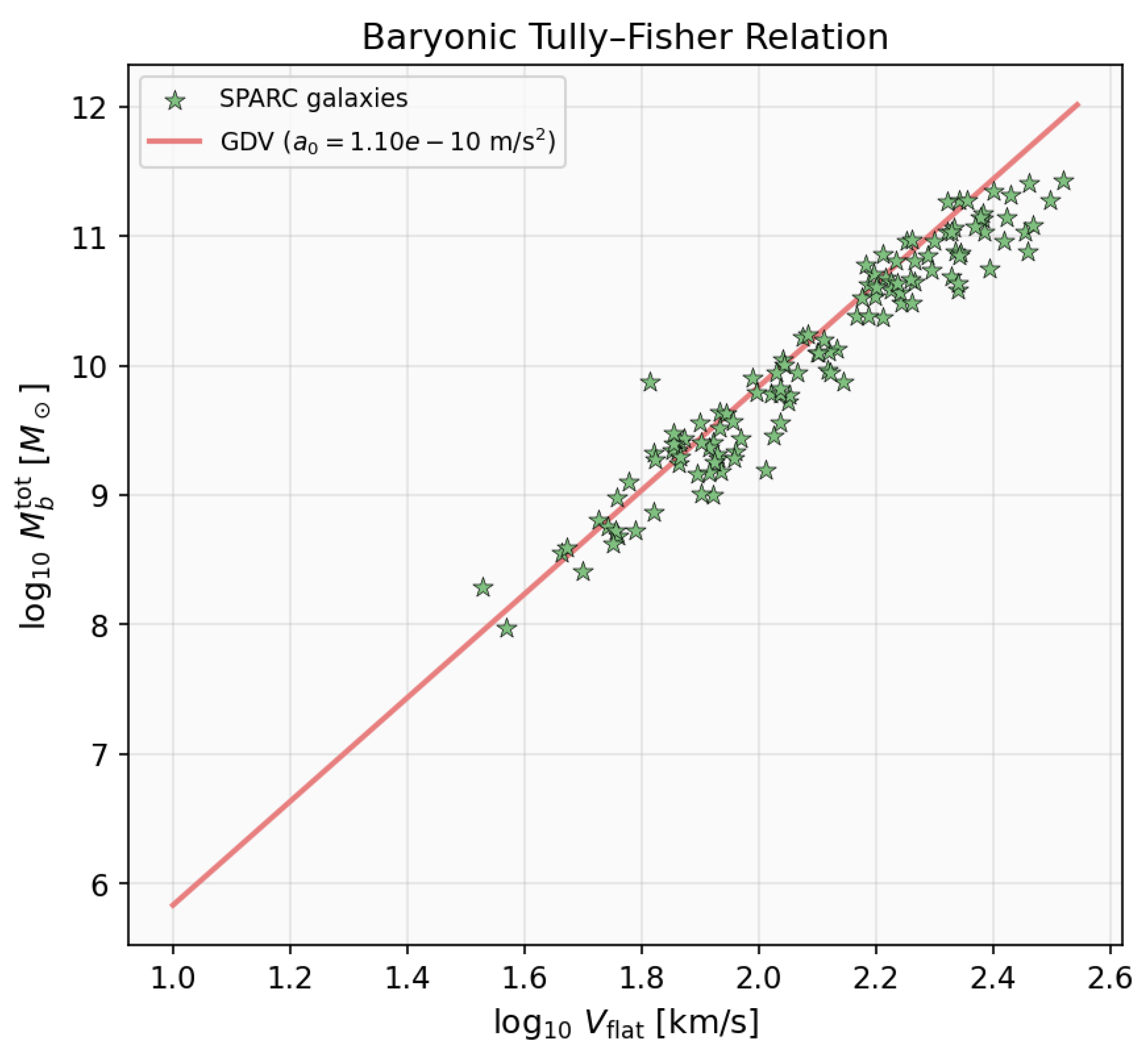
6.3.1. Cosmological Interpretation

Using the GDV cosmological relation between $a_0$ and $\beta$, we obtain

$$\beta \simeq 5.8\times {10}^{-3}.$$

(229)

These results demonstrate that the GDV model provides a priori quantitative predictions in agreement with galactic rotation curves, without invoking dark matter halos or empirical fitting functions.

Figure 2. Galaxy Rotation Curves of NGC3521 and UGC06917.

Figure 2. Galaxy Rotation Curves of NGC3521 and UGC06917.

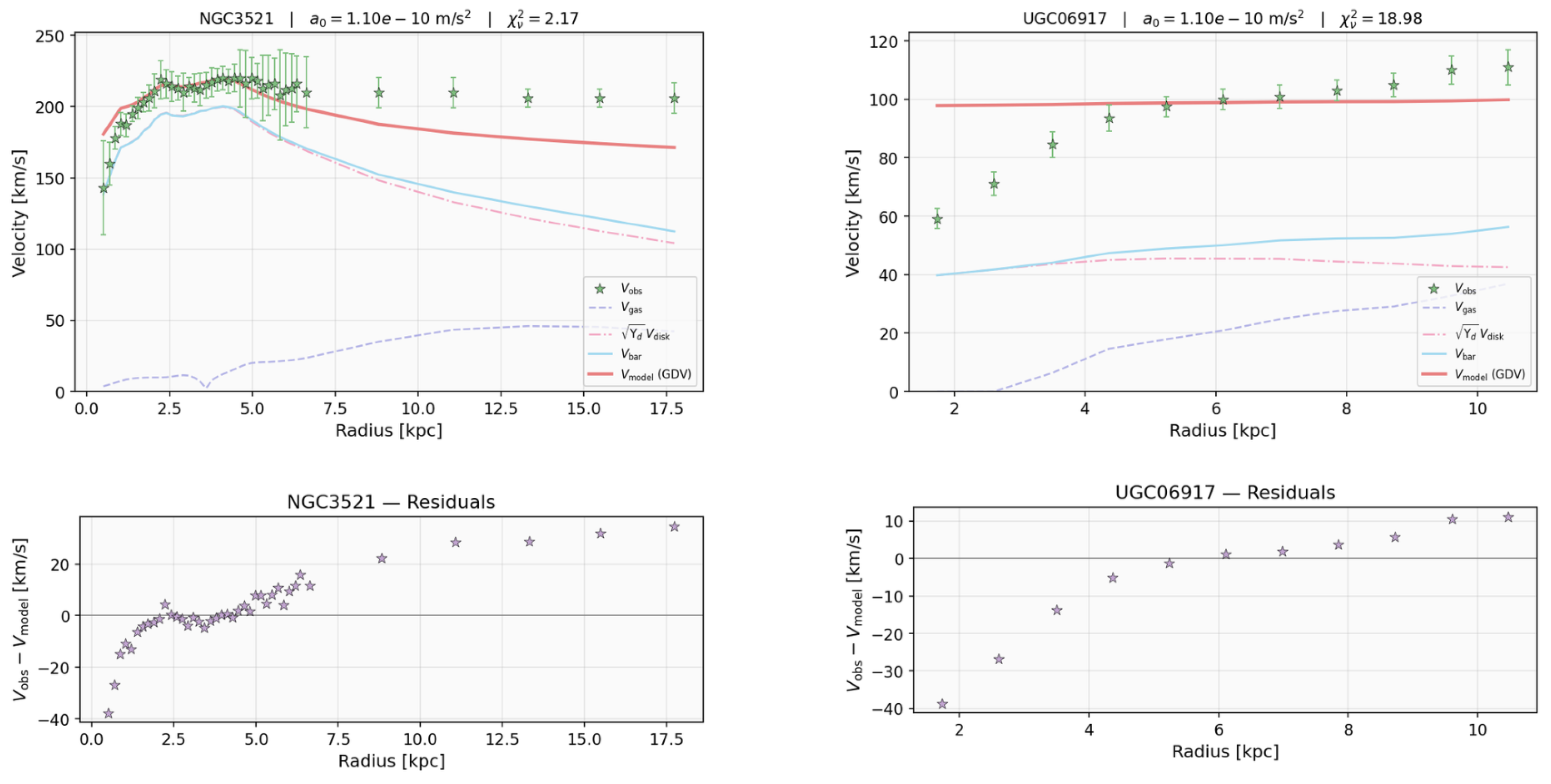
Figure 3. Galaxy Rotation Curves of NGC5005 and UGC07690.

Figure 3. Galaxy Rotation Curves of NGC5005 and UGC07690.

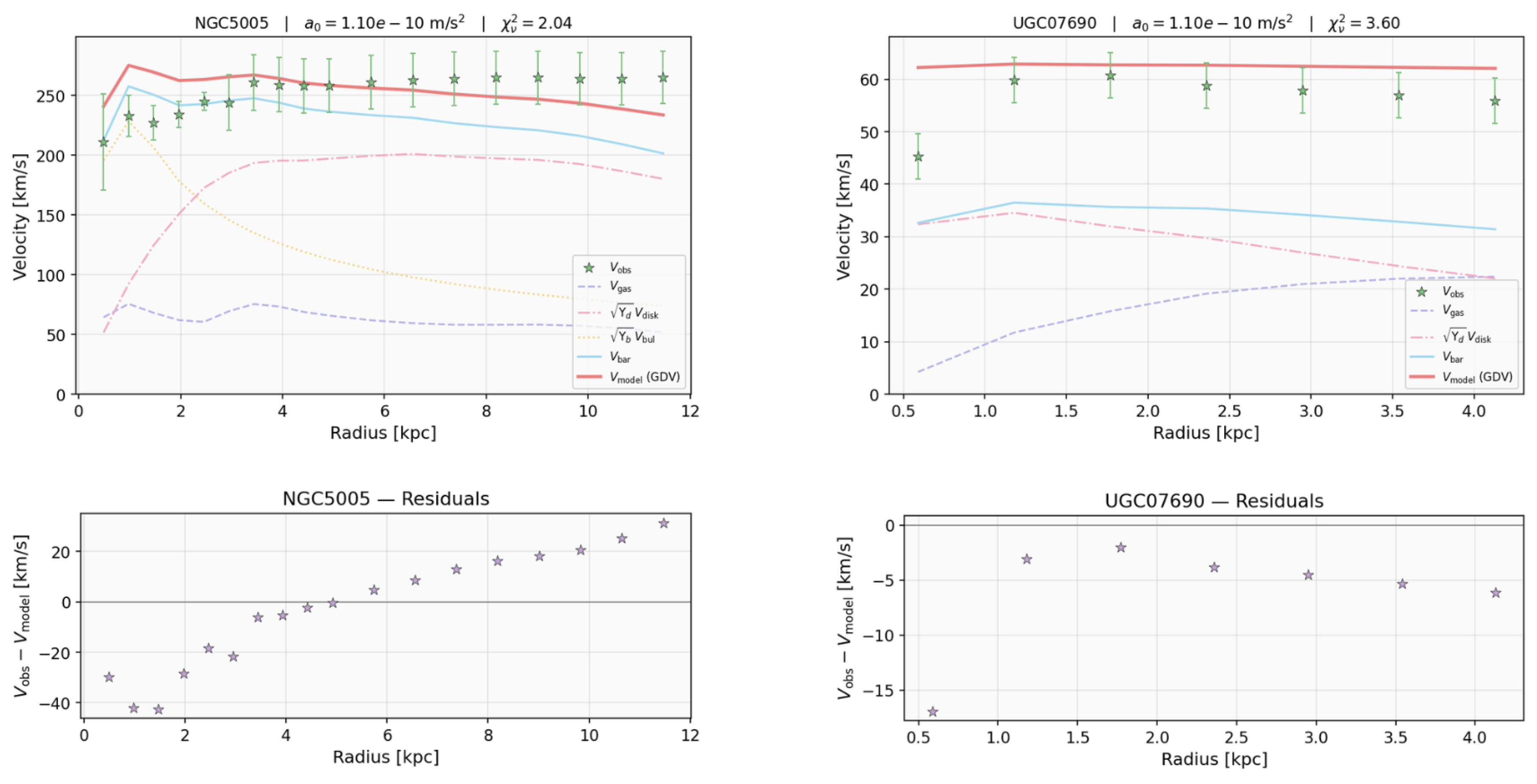
6.4. Comparison with MOND and $\Lambda$CDM

Both GDV and MOND reproduce the baryonic Tully–Fisher relation,

$$v^4\propto M_b,$$

(230)

in the deep modified regime. However, GDV fundamentally differs the acceleration scale $a_0$ from cosmological vacuum dynamics, whereas deep MOND treats $a_0$ as an empirical universal constant without microphysical origin.

In the standard $\Lambda$CDM model,

$$v^2\left(r\right)={\displaystyle \frac{G\left(M_b\left(r\right)+M_{\mathrm{DM}}\left(r\right)\right)}{r}},$$

(231)

requiring massive and highly fine-tuned dark matter halos, especially in ultra-diffuse and isolated dwarf galaxies. By contrast, the GDV model requires no dark matter. It is able to predicts galaxy rotation curves using a single cosmologically derived parameter $a_0$. It naturally explains the dynamics of isolated UDGs without excessive halo masses. Finally, GDV introduces a well-defined environmental dependence through $b\left(t\right)$.

The GDV rotation curve model possesses the following fundamental GDVantages. $a_0$ is a derived cosmological quantity, not a phenomenological fit. The baryonic Tully–Fisher relation is kept as an exact theoretical consequence. The model establishes a direct link between cosmic expansion, torsion-driven vacuum dynamics, and galactic rotations.

These results establish the GDV framework as a predictive, and cosmologically grounded alternative to both MOND and the $\Lambda$CDM paradigm.

7. Discussion

7.1. The Coincidence Problem as a Geometric Phase Transition

A persistent conceptual challenge in modern cosmology is the so–called cosmic coincidence problem, namely the question of why the energy densities associated with matter and late–time acceleration are of the same order of magnitude at the present epoch. Within the standard $\Lambda$CDM framework, this near equality appears accidental: while the matter density scales as ${\rho }_m\propto a^{-3}$, the dark energy density is introduced as an external constant, ${\rho }_{\Lambda }=\mathrm{const}$. The present–day balance therefore requires a fine tuning of the initial value of $\Lambda$, with no internal mechanism selecting the epoch at which ${\rho }_m\sim {\rho }_{\Lambda }$.

In the GDV framework, the coincidence problem admits a qualitatively different interpretation. The drift–induced contribution does not constitute an independent fluid component competing with matter in the cosmic energy budget. Instead, it arises as a geometric response of spacetime itself, generated by the torsion–trace sector of the action. As shown explicitly in Section 3, the associated energy density is a variational consequence of the quadratic torsion–trace term and is functionally tied to the expansion history through $H\left(t\right)$ and $a\left(t\right)$, rather than being specified by an external constant.

More precisely, the GDV contribution scales with the square of the effective expansion rate, ${\rho }_{\mathrm{GDV}}\propto H_{\mathrm{eff}}^2$. As a result, the ratio ${\rho }_{\mathrm{GDV}}/{\rho }_m$ is not freely adjustable, but is governed by the dynamical evolution of the Hubble parameter. At early times, when H is large and the expansion is dominated by the homogeneous background, the geometric drift contribution is parametrically suppressed relative to matter. At late times, as the expansion rate decreases and the universe enters the low–acceleration regime, the torsion–trace response becomes increasingly relevant. The near equality ${\rho }_{\mathrm{GDV}}\sim {\rho }_m$ therefore signals a transition in the geometric regime of the manifold rather than a stochastic alignment of unrelated components.

From this viewpoint, the coincidence problem is reformulated as a geometric phase transition. The epoch at which the drift contribution becomes dynamically important is set by the evolution of $H\left(t\right)$ itself, rather than by an externally tuned energy scale. Unlike $\Lambda$CDM, where the onset of acceleration is fixed by the value of a constant vacuum energy, the GDV framework ties the emergence of late–time acceleration directly to the expansion history of the universe. The coincidence is thus not eliminated by fine tuning, but rendered inevitable by the structure of the theory.

This geometric reinterpretation also clarifies the Machian aspect of the model. While the present framework does not require a time–varying gravitational constant, it naturally allows for an interpretation in which the effective strength of gravity reflects the global geometric state of spacetime. Any such modulation is strongly suppressed at early times and in high– density environments, ensuring consistency with primordial nucleosynthesis and Solar System tests. At late times and on large scales, however, the same geometric coupling underlies the emergence of both drift–induced acceleration and the observed coincidence.

In this sense, the cosmic coincidence ceases to be a fine–tuning problem and instead becomes a diagnostic of the transition between geometrically distinct expansion regimes. The balance observed today is not accidental, but a direct manifestation of the torsion–driven response of spacetime to its own expansion history.

7.2. On the Interpretation of G

In Newtonian mechanics, the gravitational interaction is characterized by the universal Cavendish constant G. General Relativity preserves this role by introducing G as the coupling constant between spacetime geometry and the energy–momentum tensor in the Einstein field equations.

In a homogeneous and isotropic FLRW background, the cosmic acceleration is governed by [19]

$${\displaystyle \frac{\ddot{a}}{a}}=-{\displaystyle \frac{4\pi G}{3}}\sum _i{\rho }_i(1+3w_i),$$

(232)

which explicitly relates the expansion dynamics of the Universe to the gravitational coupling and the total energy content. This equation shows that, within standard cosmology, the large–scale dynamics of spacetime are controlled by the same constant G that governs local gravitational interactions.

Within a generalized Machian perspective, however, the strength of local gravity need not be viewed as an entirely fundamental input. Instead, it may be regarded as an effective coupling emerging from the global inertial state of the Universe. In this interpretation, the distribution of matter and the kinematic state of the manifold influence how strongly local systems respond to gravity, without requiring any modification of the local field equations.

This viewpoint can be illustrated by considering two hypothetical universes with identical expansion histories $a\left(t\right)$ but different total mass densities. If the cosmic acceleration $\ddot{a}$ is fixed, a larger background density requires a smaller effective coupling in the acceleration equation. This does not imply that the locally measured Cavendish constant varies in time or space, but rather that the effective gravitational response of local systems is screened by the global inertial background. Such a mechanism may be described as a Machian screening of gravity.

Unlike scalar–tensor theories such as Brans–Dicke gravity, where the variation of G is governed by an independent scalar field, the present framework does not promote G itself to a dynamical degree of freedom. Instead, any apparent modulation of the gravitational coupling arises indirectly through the geometric drift sector, encoded in the torsion–trace contribution of the GDV tetrad. In the local Solar–System limit, where the drift parameter satisfies $b\to 0$ and $a\to 1$, the standard value of G is recovered exactly, ensuring consistency with high–precision gravitational experiments.

At cosmological scales, the situation is qualitatively different. The presence of a nonvanishing torsion trace modifies the effective acceleration governing large–scale dynamics, leading to deviations from the standard Friedmann behavior. In this sense, the GDV framework allows the gravitational interaction to appear stronger or weaker depending on the global expansion state of the Universe, without violating local conservation laws or introducing new fundamental constants.

It is important to emphasize that a contracting universe ($\ddot{a}<0$) does not imply a repulsive gravitational interaction within the present framework. Rather, any effective repulsive behavior must arise from the geometric contributions associated with the torsion trace, corresponding to ${\rho }_{\mathrm{eff}}+3p_{\mathrm{eff}}<0$ in the effective description. This distinction is crucial for maintaining consistency with the standard interpretation of the Friedmann equations.

Overall, the GDV framework suggests a deeper connection between inertia, global matter distribution, and the effective strength of gravity. While G remains a constant parameter at the level of local physics, its cosmological role may be understood as emergent, reflecting the dynamical state of spacetime itself.

7.3. On the Interpretation of Inertia

Newton thought that falling bodies are under the influence of a gravitational force, and therefore considered this motion to be an accelerated/forced motion (that is, he believed that bodies are genuinely being pulled). However, in the thought experiment that Einstein called “The happiest thought of my life was: that the observer in free fall does not feel his own weight, (Der glücklichste Gedanke meines Lebens war: dass der Beobachter im freien Fall sein eigenes Gewicht nicht spürt)”. He realized that bodies falling toward the ground actually fall without feeling any force. From this, the following conclusion can be drawn from Einstein’s general relativity: in reality, bodies are not falling; rather, the observer on the ground is accelerating toward them, and therefore measures their motion as accelerated. (For example, according to Newton, all circular motions are accelerated; therefore, all bodies in orbit are non-inertial. According to Einstein, however, if the geodesics of spacetime are elliptical and a body travels along these elliptical curves, then that body is inertial.) From this interpretation, a connection can be established between gravitation and acceleration. However, Einstein first employed Riemannian geometry in doing so. In this framework, large masses cause geometric curvatures that cannot be neglected. Yet in the equivalence principle, Einstein believed that gravitation and acceleration were intrinsically connected in origin, and at times he even thought of them as identical. Nevertheless, realizing that gravity bends spacetime in a Riemannian sense, whereas acceleration does not bend real spacetime and is instead a “coordinate effect,” bothered Einstein at the level of principle. While trying to unify these two quantities, Einstein ended up completely separating them. In our approach, by contrast, acceleration and gravitation arise from a single fundamental origin. In one case, we accelerate; in the other, we experience compatibility or incompatibility with the dynamics of the universe. In fact, all of this has a single origin: inertia.

8. Conclusion

In this work, we have developed a drift-adapted tetrad formulation within teleparallel gravity in which gravitational effects are described in terms of the inertial (kinematic) structure of spacetime. Within this framework, both local gravitational phenomena and large-scale cosmological dynamics originate from a common geometric ingredient — the spatial drift field $W^i$.

The key element of the construction is the inertial structure defined by a natural congruence. Deviations between an observer frame and this structure give rise to effective force terms. The drift-tetrad formulation encodes this relation covariantly through the torsion trace. The theory preserves full diffeomorphism invariance and local Lorentz covariance; the torsion trace and the scalars derived from it are geometrically well-defined quantities rather than coordinate artifacts.

The drift field admits a natural decomposition into global and local components. The global sector governs homogeneous cosmic expansion, while the local sector captures matter-induced deviations. In this way, cosmic acceleration and galactic-scale modifications arise within a single geometric ansatz, without introducing additional dark degrees of freedom.

The central quantity entering the quadratic sector of the action is the projection of the torsion trace along the natural observer congruence,

$$\mathcal{S}=T_{\mu }{u}^{\mu }.$$

(233)

This scalar measures the difference between the metric expansion rate and the drift expansion rate. Its quadratic contribution generates effective energy density and pressure terms. The Hamiltonian constraint analysis indicates that the GDV sector does not introduce additional propagating degrees of freedom beyond those of teleparallel gravity.

At the cosmological level, the torsion-trace contribution behaves as an effective geometric fluid. In the quasi-static regime it resembles a curvature-like term, while the full dynamical evolution admits late-time accelerated solutions without an explicit cosmological constant. The corresponding energy scale is determined by the drift parameters, providing a geometrically controlled mechanism for accelerated expansion.

At galactic scales, the local drift contribution leads to an effective density profile

$${\rho }_{\mathrm{GDV}}\propto r^{-2},$$

(234)

which produces asymptotically flat rotation curves and reproduces the Baryonic Tully–Fisher scaling relation. The associated acceleration scale $a_0$ is determined by cosmological drift parameters rather than by an empirical interpolation function. In this sense, MOND-like behavior arises as a regime of the underlying torsion-based dynamics.

The theory remains consistent with high-precision local tests. In the static vacuum limit $b\to 0$, the Schwarzschild solution is recovered together with the standard post-Newtonian parameters $\gamma =\beta =1$ and vanishing torsion trace. Tensor perturbations propagate at luminal speed and no additional polarizations appear, ensuring compatibility with gravitational-wave constraints. The model therefore exhibits consistent behavior at Solar-System, galactic, and cosmological scales.

Conceptually, the formulation relates gravitational effects to the inertial structure encoded in the drift field. Rather than introducing separate dark components, the framework provides a covariant geometric extension of teleparallel gravity in which cosmological acceleration and galactic-scale modifications originate from the same torsion-trace sector.

Further detailed confrontation with cosmological and astrophysical data will determine the quantitative viability of this scenario.

References

- Einstein, A. Math. Ann. 1930, 102, 685. [CrossRef]
- Komatsu, E.; Dunkley, J.; Nolta, M. R.; Bennett, C. L.; Gold, B.; Hinshaw, G.; Wright, E. L. Five-year wilkinson microwave anisotropy probe observations: cosmological interpretation. The Astrophysical Journal Supplement Series 2009, 180(2), 330–376. [Google Scholar] [CrossRef]
- Capozziello, S.; Caruana, M.; Farrugia, G.; Levi Said, J.; Sultana, J. Cosmic growth in f (T) teleparallel gravity. General Relativity and Gravitation 2024, 56(2), 27. [Google Scholar] [CrossRef]
- Geng, C. Q.; Lee, C. C.; Saridakis, E. N.; Wu, Y. P. “Teleparallel” dark energy. Physics Letters B 2011, 704(5), 384–387. [Google Scholar] [CrossRef]
- Carroll, S. M.; Duvvuri, V.; Trodden, M.; Turner, M. S. Is cosmic speed-up due to new gravitational physics? Physical Review D 2004, 70(4), 043528. [Google Scholar] [CrossRef]
- Capozziello, S.; Carloni, S.; Troisi, A. Quintessence without scalar fields. arXiv 2003. [Google Scholar] [CrossRef]
- De Felice, A.; Tsujikawa, S. f (R) theories. Living Reviews in Relativity 2010, 13(1), 1–161. [Google Scholar] [CrossRef] [PubMed]
- Cai, Y. F.; Capozziello, S.; De Laurentis, M.; Saridakis, E. N. f (T) teleparallel gravity and cosmology. Reports on Progress in Physics 2016, 79(10), 106901. [Google Scholar] [CrossRef] [PubMed]
- Krššák, M.; Saridakis, E. N. The covariant formulation of f (T) gravity. Classical and Quantum Gravity 2016, 33(11), 115009. [Google Scholar] [CrossRef]
- Bengochea, G. R.; Ferraro, R. Dark torsion as the cosmic speed-up. Physical Review D—Particles, Fields, Gravitation, and Cosmology 2009, 79(12), 124019. [Google Scholar] [CrossRef]
- Hawking, S. W.; Ellis, G. F. The large scale structure of space-time; Cambridge university press, 2023. [Google Scholar]
- Kiefer, C. Quantum Gravity: Third Edition; OUP Oxford: United Kingdom, 2012. [Google Scholar]
- Carlip, S. General relativity: a concise introduction; Oxford University Press, 2019. [Google Scholar]
- Bhattacharya, S.; Dialektopoulos, K. F.; Romano, A. E. Eur. Phys. J. C 2017, 77, 526. [CrossRef]
- Carrera, M.; Giulini, D. Rev. Mod. Phys. 2010, 82, 169. [CrossRef]
- Lelli, F.; McGaugh, S. S.; Schombert, J. M. SPARC: Mass models for 175 disk galaxies with Spitzer photometry and accurate rotation curves. The Astronomical Journal 2016, 152(6), 157. [Google Scholar] [CrossRef]
- Particle dark matter: observations, models and searches; Bertone, G., Ed.; Cambridge University Press, 2010. [Google Scholar]
- Hayashi, K.; Shirafuji, T. New general relativity. Physical Review D 1979, 19(12), 3524. [Google Scholar] [CrossRef]
- Mukhanov, V. Physical Foundations of Cosmology; Cambridge University Press: Cambridge, 2005. [Google Scholar]
- Milgrom, M. A modification of the Newtonian dynamics as a possible alternative to the hidden mass hypothesis. Astrophysical Journal Research supported by the US-Israel Binational Science Foundation. 1983, 270, 365–370. [Google Scholar] [CrossRef]
- Milgrom, M. The a0–cosmology connection in MOND. arXiv 2020, arXiv:2001.09729. [Google Scholar]
Disclaimer/Publisher’s Note: The statements, opinions and data contained in all publications are solely those of the individual author(s) and contributor(s) and not of MDPI and/or the editor(s). MDPI and/or the editor(s) disclaim responsibility for any injury to people or property resulting from any ideas, methods, instructions or products referred to in the content. |
© 2026 by the authors. Licensee MDPI, Basel, Switzerland. This article is an open access article distributed under the terms and conditions of the Creative Commons Attribution (CC BY) license (http://creativecommons.org/licenses/by/4.0/).
Copyright: This open access article is published under a Creative Commons CC BY 4.0 license, which permit the free download, distribution, and reuse, provided that the author and preprint are cited in any reuse.