
Submitted:
15 December 2025
Posted:
16 December 2025
You are already at the latest version
Abstract
This study proposes and systematically validates a new analytical wake model that incorporates atmospheric stability effects. By introducing a stability-dependent turbulence expansion term with a square of a cosine function and the stability sign parameter, the model dynamically responds to varying atmospheric conditions, overcoming the reliance of tranditional models on neutral atmospheric assumptions. It achieves physically consistent descriptions of turbulence suppression under stable conditions and convective enhancement under unstable conditions. A newly developed far-field decay function effectively coordinates near-wake and far-wake evolution, maintaining computational efficiency while significantly improving prediction accuracy under complex stability conditions. The Present model has been validated against field measurements from the Scaled Wind Farm Technology (SWiFT) facility and the Alsvik wind farm, demonstrating superior performance in predicting wake velocity distributions on both vertical and horizontal planes. It also exhibits strong adaptability under neutral, stable, and unstable atmospheric conditions. This proposed framework provides a reliable tool for wind turbine layout optimization and power output forecasting under realistic atmospheric stability conditions.
Keywords:
wind turbine
; wake
; velocity deficit
; analytical model
; atmospheric stability
1. Introduction
As a crucial component of clean and renewable energy, wind energy is playing an increasingly important role in the global energy transition. With the continuous development of wind power, wind farm layout optimization and operational efficiency improvement have become key research priorities. Among the various challenges involved, the wake effect between wind turbines stands out as a core factor affecting overall wind farm performance. The wake leads to reduced incoming wind speed and increased turbulence intensity for downstream turbines, consequently causing power losses and structural fatigue damage. Therefore, accurate prediction of wind turbine wake characteristics is of significant scientific and engineering importance for the micro-siting, power prediction, and lifetime assessment of wind farms [1].
From the perspective of atmospheric structure, as noted by Cermak and Cochran [2], the atmosphere within approximately 1000 meters above the ground surface typically constitutes the atmospheric boundary layer. The lowest 100 meters of boundary layer is defined as the atmospheric surface layer. Recently, to enhance wind energy capture efficiency and conserve land or sea resources, the wind power industry has been actively advancing the design and development of large-scale wind turbines [3]. Since 2019, when the hub height of offshore wind turbines surpassed 103m and the rotor diameter reached 150m [4], the industry has entered a phase of accelerated advancement. By the end of 2025, the world’s first 26 MW offshore wind turbine with hub height of 185 meters and rotor diameter of 310 meters has been successfully connected to the grid in Shandong Province, China. This trend indicates that modern wind turbines now operate beyond the atmospheric surface layer, and their aerodynamic performance is increasingly dependent on physical processes throughout the entire atmospheric boundary layer. Therefore, as a key factor governing wind shear, turbulent mixing, and energy transfer within the boundary layer, atmospheric stability is of growing importance in wind turbine wake assessment.
Atmospheric stability is generally categorized into stable, neutral, and unstable conditions. Under unstable atmospheric conditions, the air warmer than the surrounding environment expands and rises, promoting vertical development of turbulence to considerable heights. Under neutral atmospheric conditions, the air at the same temperature as its environment remains at its original height, resulting in only weak mixing [5]. Under stable atmospheric conditions, the cooler air compresses and sinks, suppressing vertical motion and weakening vertical mixing [6]. By directly influencing the wind speed profile and turbulence structure, atmospheric stability governs the recovery rate and spatial diffusion of wind turbine wakes ([7,8,9,10,11,12,13,14]). Both field measurements and high-fidelity numerical simulations illustrate that the spatial distributions of wake velocity deficit and added turbulence intensity under different atmospheric stability conditions show significant differences. As demonstrated by Pérez et al. [15], the annual energy production (AEP) vary by more than 16% under different stability conditions. Specifically, under stable conditions, the wind turbine wake recovers slowly , resulting in a persistent velocity deficit over a long downstream distance which leads to a lower AEP. In contrast, under unstable conditions, intense turbulent mixing facilitates faster wake recovery, yielding a higher AEP. Therefore, incorporating atmospheric stability into wake models is essential for improving wake prediction accuracy, enabling refined assessment of wind resources, and ensuring structural safety of turbines.
Traditional wake models, such as the classic Jensen (PARK) model and its derivatives, rely mostly on the assumption of neutral atmospheric conditions and depend heavily on empirical parameters. This limitation is typically exemplified by the variability of the wake decay coefficient in the Jensen model across different wind farms. Peña et al. [16] found that in Sexbierum case, the wake decay coefficient of the Jensen model should be adjust from the typical onshore value of 0.075 to a site-specific value of 0.038. In response, some researchers have focused on quantifying the wake decay coefficient. Cheng and Porté-Agel [17] proposed a physics-based wake model, drawing on scalar dispersion in turbulence. This model, accounts for the influence of ambient turbulence intensity based on Taylor’s diffusion theory. Vahidi and Porté-Agel [18] developed a physics-based model by introducing a filtered turbulence scale to account for the combined effects of ambient and turbine-induced turbulence. Bastankhah and Porté-Agel [19] proposed a concise analytical wake model based on the conservation of mass and momentum and a Gaussian-shaped velocity deficit, which requires a wake growth rate parameter to determine the wake velocity. Building upon this, Niayifar and Porté-Agel [20] further enhanced the model by determining the wake growth rate from the local streamwise turbulence intensity. It should be noted that the key empirical constant was derived via linear regression of Large Eddy Simulation (LES) data, and its agreement with field measurements requires further validation. Ishihara and Qian [21] estiblished a relationship linking the standard deviation of the Gaussian distribution to the turbine thrust coefficient and the incoming turbulence intensity, thereby overcoming the reliance on empirical parameters in wake models. Nevertheless, such modified models are proposed under neutral atmospheric conditions and their applicability should be further verified.
Recently, some researchers have focused on incorporating atmospheric stability into wake models for a more comprehensive assessment of wind turbine wakes, with the main methodologies falling into two categories: methods based on numerical simulations and methods involving the modification of previous analytical wake models. In the realm of numerical simulations, Kale et al. [22,23] employed LES within the Weather Research and Forecasting Model (WRF) framework with Monin-Obukhov similarity theory to generate stable and unstable atmospheric boundary layers, using an actuator disk model for turbine simulation. They investigated the aerodynamic characteristics of full-scale wind turbines under different atmospheric conditions using a generalized actuator disk model. However, this approach is computationally expensive. Furthermore, under stable stratification, it exhibits significant deviations in wake velocity deficit and delayed wake recovery due to low turbulence intensity, high wind shear, and wind veer. Nygaard et al. [24] developed a simplified two-dimensional Reynolds-Averaged Navier-Stokes (RANS) model based on the Boussinesq buoyancy approximation, which incorporates vertical energy transfer under different stability conditions by simplifying the governing equations into a parabolic form. This method qualitatively reproduces the influence of updrafts and downdrafts on the wake, but prioritizes mechanistic insight over quantitative accuracy.
Compared to methods based on numerical simulations, some researchers have devoted efforts to a more concise and practical methodology: directly incorporating atmospheric stability parameters into analytical wake models. Emeis [25] developed a top-down wind park model that integrates atmospheric stability effects on both momentum flux and momentum loss. Although it quantifies the macroscopic impact of atmospheric stability on the velocity deficit at hub height, it fails to capture the dynamics of individual turbine wakes and wind direction shifts. Abkar and Porté-Agel [26] characterizes the differential growth of the wake in the lateral and vertical directions under different atmospheric conditions using a two-dimensional elliptical Gaussian distribution, in which wake growth rates were obtained by fitting LES results. Han et al. [27] established a simple logarithmic model linking wake expansion to turbulence, thereby indirectly incorporating atmospheric stability. While efficiently captures key wake features, this model lacks an explicit stability parameter and performs poorly in the near-wake region under very low turbulence intensity. Cheng et al. [28] linked atmospheric stability to the lateral turbulence intensity and proposed a linear relationship between the lateral turbulence intensity and the wake expansion rate. However, as the authors noted, the model possesses inherent limitations in the near-wake region and under low incoming turbulence intensity. Xiao et al. [29] proposed the 3D-Stability-COUTI model, which incorporates the Obukhov length to predict wakes under different atmospheric stability conditions without empirical tuning. While accurate in general, its summation of two cosine functions results in an overemphasis of the bimodal velocity structure in the near-wake region under stable atmospheric conditions with low turbulence intensity and high wind shear.
Overall, the two aforementioned methodologies for incorporating atmospheric stability into wake models present distinct advantages and limitations. High-fidelity numerical methods like LES can directly resolve turbulent structures and wake expansion under different atmospheric stability conditions, offering clear physical mechanisms and broad applicability. However, their high computational cost limits their practicality for routine engineering applications. In contrast, modified analytical wake models include atmospheric stability parameters like the Monin-Obukhov length to approximate atmospheric stability effects to maintain computational efficiency. Nevertheless, their capacity to describe nonlinear responses under stable atmospheric stability conditions remains limited.
In summary, while progress has been made in establishing wake models considering atmospheric stability, several limitations are still exist: (i) Traditional models exhibit significant deviations in predicting wake velocity deficit and wake recovery process under stable atmospheric conditions; (ii) Most wake models lack a unified framework that is both adaptable to different atmospheric stability conditions and capable of sustaining high prediction accuracy throughout both the near-wake and far-wake regions; (iii) Key parameters in analytical wake models considering atmospheric stability often require case-specific calibration. These limitations urgently call for the development of a new generation of wake prediction methodologies: First, a atmospheric stability parameterization scheme should be established based on atmospheric boundary layer theory to accurately describe velocity profiles and the wake recovery process. Second, it is necessary to construct a unified wake prediction framework covering the entire wake region. Ultimately, by establishing functional relationships between key wake model parameters and atmospheric stability, a analytical wake model balancing physical fidelity with engineering applicability can be proposed.
Therefore, the structure of this paper is organized as follows. Section 2 proposes a new wake model considering atmospheric stability, including fundamentals of atmospheric stability, previous wake models with atmospheric stability, proposal of new wake model with atmospheric stability and methodology for prediction accuracy assessment. Section 3 provides performance assessment of the present wake model. In this section, field measurements from two cases-Vestas V27 wind turbine and Danwin 180kW wind turbine are adopted to assess wake model prediction performance. Finally, a summery and conclusions are presented in Section 4.
2. Propose of a New Wake Model Considering Atmospheric Stability
2.1. Fundamentals of Atmospheric Stability
The Monin-Obukhov Similarity Theory (MOST) [30], built upon the characteristic length scale proposed by Obukhov [31], provides a universal framework for describing the turbulent structures within the atmospheric surface layer. This length scale is defined by the relative importance of buoyant production to mechanical shear production of turbulence kinetic energy. The core of the theory lies in applying dimensional analysis to simplify the complex turbulent transfer processes into functions of a single dimensionless parameter, ζ [32]. The governing equations are given as follows [33]:
In Equation (1), is stability parameter in which is the height above the ground surface and is the Obukhov length scale. is the Karman constant. is gravitational acceleration. is a temperature scale and is mean potential temperature. is the friction velocity.
Based on the definition of stability parameter, the logarithmic wind speed can be derived as[30],
where is the non-dimentional wind shear and is the mean wind speed. To directly incorporate the Obukhov length L as a key stability parameter into the logarithmic wind speed profile, a piecewise function formulation was developed based on a series of field observations from the 1980s through dimensional analysis and empirical fitting ([34,35,36]). The following form has since become the widely adopted standard model,
where . As illustrated by Monin and Obukhov [30], with stable stratification, the turbulent heat flux is directed downward, ; while unstable stratification on the other hand, ; with neutral stratification, . According to surface layer theory [37], the following relationship can be derived for the surface layer over flat and homogeneous terrain,
where is the wind speed at height . Dividing by the wind speed at the hub height, , eliminates and yields the following equation for the incoming flow wind speed profile that accounts for atmospheric stability,
where . Similarly, the incoming flow turbulence intensity profile that accounts for atmospheric stability,
where is the turbulence intensity at the hub height. Therefore, this derivation enables the calculation of the incoming flow wind speed and turbulence intensity profiles via Equations (5) and (6), using the hub-height wind speed and turbulence intensity obtained from nacelle-based sensors such as LiDAR or 3D scanning LiDAR.
2.2. Previous Wake Models with Atmospheric Stability
In this study, two previous wake models considering atmospheric stability, 3D-Stability-COUTI [29] and Cheng2019 [28], are adopted for comparison with the present wake model. A brief review of the two wake models is provided below to establish a foundation for the subsequent comparative analysis.
Xiao et al. [29] proposed an integrative three-dimensional cosine-shaped analytical model, named 3D-Stability-COUTI, for characterizing wake velocity and turbulence intensity under varying atmospheric stability conditions. Firstly, the essential input parameters for calculating the velocity deficit encompass the wind turbine specifications, atmospheric inflow conditions and terrain characteristics, as shown in Table 1.
Then, according to Table 1, the wind speed, , and turbulence intensity, , at hub height are essential input parameters for deriving the incoming wind velocity and turbulent intensity profiles via Equations (5) and (6) considering atmospheric stability.
After that, the wake radius at any downstream position is determined using a stability-corrected wake width model that incorporates the Obukhov length, it is defined as follows,
where is the rotor diameter. is the Karman constant. is the thrust coefficient. is streamwise, spanwise and vertical coordinates, respectively.
The third step focuses on predicting the wake velocity at any downstream position through a two-stage process: a prediction step that calculates the 1D average wake velocity deficit , shown in Equation (9) and a correction step that redistributes in 3D space using a dual-cosine shape function, shwon in Equation (10) to obtain the detailed velocity deficit distribution , shown in Equation (11). Finally, the wake velocity at any position in the wake field is provided by combining the incoming wind velocity with the calculated velocity deficit distribution, shown in Equation (12).
where . is the half width of the single-peak deficit profile, calculated by . represents the radial distance from the wake centerline to the location of the maximum single-peak deficit, which is determined empirically as . is functionally dependent on and is computed as . is the radial distance from the wake center position .
Cheng et al. [28] incorporated the Obukhov length into the parameterization of the lateral turbulence intensity to account for the effects of atmospheric stability. This wake model, referred to herein as Cheng2019 model, requires the input parameters listed in Table 1. The incoming velocity and turbulence intensity profiles are calculated using Equations (5) and (6). Then, the lateral turbulence intensity , a parameter critical to wake expansion, is determined using the recommendation of ESDU (Equation (13)), which incorporations Coriolis effects via boundary layer height estimation. Based on this, the wake expansion rate is uniquely related to through a linear empirical formula given in Equation (15). Consequently, the intercept in the wake width growth function is derived as a function of , as presented in Equation (16). The standard deviation of the Gaussian wake profile is then obtained from and using Equation (17). The velocity deficit across the wake is subsequently computed with the Gaussian-shaped distribution, formulated in Equation (18). Finally, the wake velocity at any position in the wake field is calculated by combining the above results via Equation (12).
where is the incoming turbulence intensity. is the boundary layer height, which is estimated by,
where is the Coriolis parameter, in which is the angle of latitude and rad/s is a constant presenting the angular rotation of the Earth.
2.3. Proposal of New Wake Model with Atmospheric stability
To enhance the applicability of wake model under different atmospheric stability conditions, an improved analytical wake model is proposed in this study, termed the Present model. The Present model employs Monin-Obukhov similarity theory (Equations (5) and (6)) to determine the incoming wind speed profile and turbulence intensity profile . Furthermore, a key improvement in the Present model is the refined parameterization of wake width and velocity deficit. By introducing a sign control parameter, , directly linked to atmospheric stability conditions, the model effectively characterizes the distinct physical mechanisms of wake expansion and recovery under stable and unstable conditions.
Specifically, the equations for calculating wake width in the Present model remains consistent with that in 3D-Stability-COUTI (Equations (7) and (8)). However, the range of values for the velocity deficit has been modified from and in 3D-Stability-COUTI to . Concurrently, the velocity deficit formula has been revised from the sum of two cosine functions in 3D-Stability-COUTI to the square of a cosine function, as shown in the following equation,
where . is far-field decay function and is the stability sign paramter, defined as follows,
The selection of as the demarcation between the near and far-wake regions is physically justified by the evolution of tip vortex dynamics and its impact on the wake structure.
During operation process of wind turbine, under the influence of turbulent fluctuations, tip vortices undergo random displacements that amplify with downstream distance (Yen et al. [38]). The wake region is commonly divided into the near-wake, the intermediate wake, and far-wake regions: in the near-wake region (<2D), large-scale vortices within the shear layer lead to a bimodal distribution of turbulence intensity. As the wake develops further into the intermediate wake (3D to 5D), the shear layer continues to expand toward the wake centerline until the far-wake regions ([39,40,41]). To accurately capture this transition in the velocity deficit decay, the far-field decay function is designed to remain unity (i.e., inactive) in the near-wake region (), thereby preserving the near-wake structure, and initiates an exponential decay beyond . This formulation effectively represents the enhanced mixing with the free-stream flow in the fully developed far-wake region, where the wake recovery is dominated by turbulent diffusion rather than organized vortex structures.
Regarding the stability sign parameter, a value of 1 is assigned under stable atmospheric conditions to represent the suppression of vertical mixing and lateral wake expansion. This is achieved by modulating the exponential term in the wake expansion model, effectively capturing the physics of turbulent diffusion. Conversely, under unstable and neutral atmospheric conditions, the stability sign parameter is set to -1 to enhance the wake expansion term. This models the accelerated wake recovery from intensified turbulent mixing, allowing wake width to dynamically respond to atmospheric stability, rather than relying solely on the empirical linear growth assumed under neutral conditions.
Furthermore, unlike the 3D-Stability-COUTI model, which constructs a bimodal velocity deficit profile through the superposition of two cosine functions, the Present model simplifies the lateral distribution of the velocity deficit by adopting a modified cosine-squared function. This modification shifts the model’s focus from characterizing the bimodal structure to a streamlined, universal description. While retaining the critical flow characteristics in the near-wake region, this approach significantly reduces mathematical complexity. By integrating this simplified velocity deficit distribution with the accurate incoming profiles and the wake width model with stability sign parameter, the Present model achieves effective wake predictions across the entire wake regions under different atmospheric stability conditions, without introducing additional empirical parameters. Consequently, it demonstrates a marked improvement in overall prediction accuracy.
To quantitatively compare the core formulations of the Present model against the 3D-Stability-COUTI and Cheng2019 models, Table 2 summarizes the key mathematical representations governing the velocity deficit, wake width, and their stability-dependent modifications for each model.
2.4. Methodology for Prediction Accuracy Assessment
To quantitatively assess the prediction accuracy of the wake models under various atmospheric stability conditions, the hit rate metric, denoted as , is adopted in this study. This metric, employed by Chen and Ishihara ([39,40]), provides a normalized measure of the agreement between model predictions and experimental observations. The hit rate is defined as follows,
where represents the th observed value from field measurements, and denotes the corresponding th predicted value obtained from the wake models. The variable indicates the total number of data points included in the comparison.
The hit rate ranges from 0 to 1, where indicates perfect agreement between predictions and measurements, and values approaching 0 signify increasing deviation. This metric is particularly suitable for evaluating wake model performance because it incorporates relative error in a normalized form, giving equal importance to errors across different velocity regimes-unlike absolute error measures, which can be dominated by high-speed data points. The application of this metric allows for a consistent and interpretable comparison of model performance across the different atmospheric stability regimes investigated in this work.
3. Performance Assessment of the Present Wake Model
3.1. Case 1: Vestas V27 Wind Turbine
This section employs field measurements of wind turbine wakes acquired under different atmospheric stability conditions at the Scaled Wind Farm Technology (SWiFT) facility in Lubbock, Texas, USA [41], for the first validation case of the Present model. The site is characterized by flat terrain and homogeneous surface cover, effectively minimizing flow distortions induced by complex topography. Wake measurements were conducted using a rear-facing, nacelle-mounted SpinnerLidar operating in a specific scanning pattern. Each full scan, completed in approximately 2 seconds, provides line-of-sight velocity estimates at 984 points distributed over a spherical surface. The field measurement data of these points were subsequently linearly interpolated onto a regular grid in the lateral (y) and vertical (z) directions with a resolution finer than 1 meter. In terms of the measurement setup, the lidar scanned the wake from 2D (D is the rotor diameter) to 5D downstream of the Vestas V27 wind turbine for both neutral and stable conditions, with a spacing of 1D between consecutive planes. Under unstable conditions, measurements were focused exclusively on 3D downstream. Further details regarding the field measurement setup are available in References [42,43]. A summary of the input parameters for Case 1 under neutral, unstable, and stable atmospheric conditions is provided in Table 3.
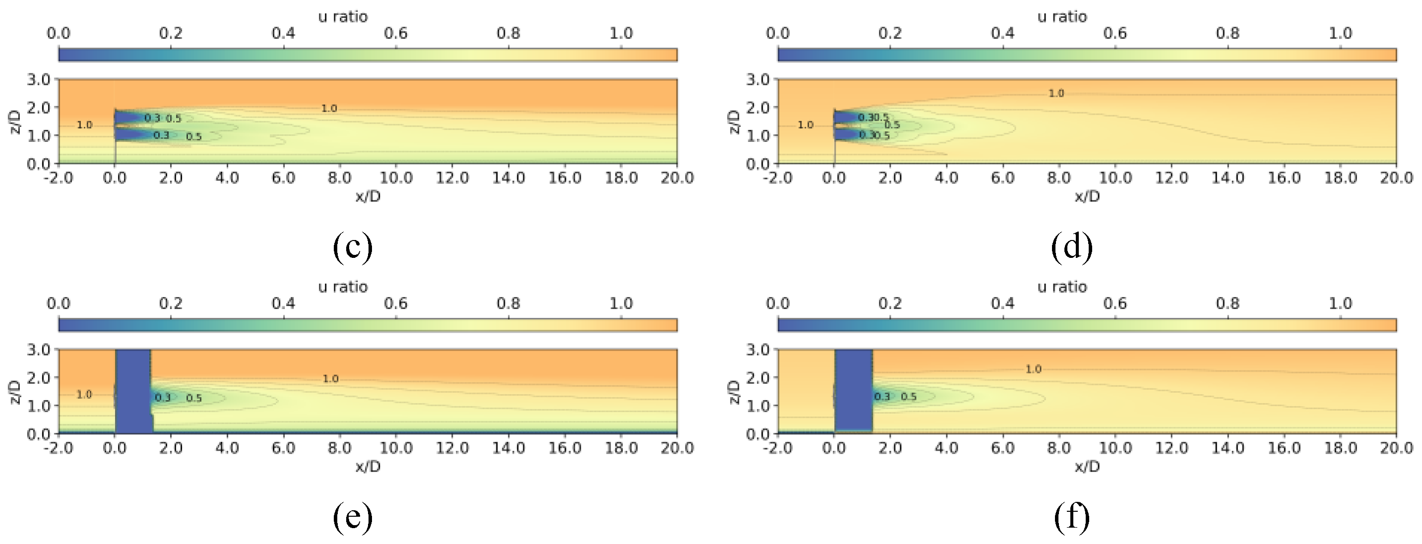
Figure 1 shows the normalized wind speed profiles along the vertical centerline () for Case 1 under stable, unstable and neutral atmospheric conditions, while Figure 2 illustrates the corresponding profiles on the horizontal plane () for the same case and stability conditions. The normolized wind speed is defined as the ratio of the local wind speed to that at the hub height, i.e., . Based on the field measurements, the vertical profiles of the wind turbine wake exhibits obvious asymmetry, which physically results from the complex interaction between turbulent mixing in the wake and the surafce effects in the near-ground region. Likewise, the horizontal profiles also display asymmetry due to the rotational motion of the the blades.
The three wake models considering atmospheric stability perform differently in capturing this asymmetric characteristic. Under stable atmospheric conditions (Figure 1(a) and Figure 2(a)), the 3D-Stability-COUTI model underestimates the velocity deficit at the hub height and produces a bimodal structure that is inconsistent with field measurements. This phenomenon is closely related to the formula of wake velocity deficit, which is defined as the sum of two cosine functions. This mathematical structure tends to overestimate the bimodal characteristics in the wake region. According to references [39,40,44], the bimodal structure in the wake is typically observed within a downstream region xtending to approximately 2D. On the other hand, the Cheng2019 model exhibits a systematic underestimation of the velocity deficit across all planes. This deviation may stem from the fact that its parameterization scheme for longitudinal turbulence intensity does not adequately respond to stable atmospheric conditions. Under unstable atmospheric conditions (Figure 1(b) and Figure 2(b)), the field measurement data are only valid on a single plane, where all three models demonstrate high prediction accuracy. Under neutral atmospheric conditions (Figure 1(c) and Figure 2(c)), both the 3D-Stability-COUTI and Cheng2019 models consistently underestimate the velocity deficit across all the planes. In contrase, the Present model agrees well with the field measurements at and 3D downstream but tends to slightly overestimate the velocity deficit at and 5D.
The validation metrics of the Present, the 3D-Stability-COUTI and Cheng2019 models on both vertical and horizontal planes under stable, unstable and neutral atmospheric conditions are presented in Figure 3. The corresponding hit rates is summarized in Table 4. The prediction accuracy of the three models exhibits notable differences across different atmospheric stability conditions. The Present model exhibits the highest consistency with field measurements across most of the planes, demonstrating superior prediction accuracy in wake velocity. And it shows particularly robust performance in capturing both wake velocity and development under stable and unstable atmospheric conditions. The 3D-Stability-COUTI model demonstrates moderate prediction accuracy, though its performance varies with atmospheric stability and shows a relatively obvious systematic deviation under stable conditions. The Cheng2019 model presents higher prediction accuracy under unstable and neutral conditions, but tends to overestimate wake velocity under stable conditions, indicating its relatively limited adaptability to different atmospheric stability conditions. Overall, all models exhibit good consistency under neutral conditions, while the Present model achieves the most outstanding prediction accuracy under stable conditions.
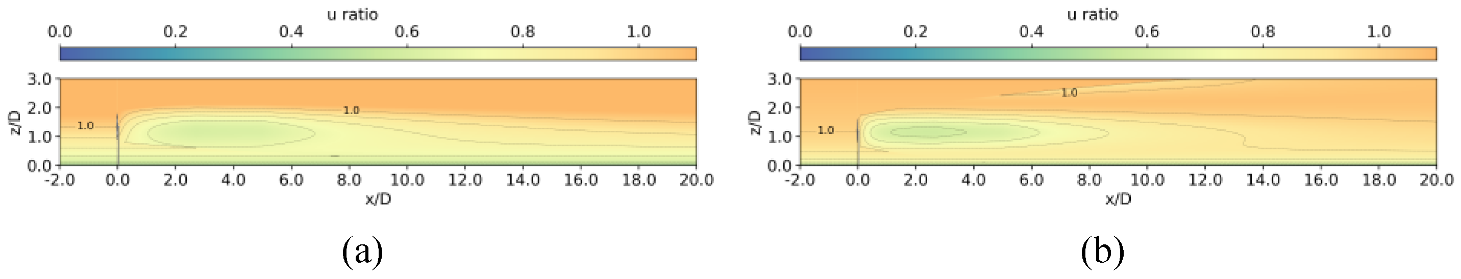
Figure 4 shows the color maps of normalized wind speed on the horizontal place at hub height for Case 1 by the Present, 3D-Stability-COUTI and Cheng2019 models under stable and unstable atmospheric conditions. It can be seen that the wake width under stable conditions is significantly narrower than that under unstable conditions-a trend that is successfully captured by all the three wake models. However, the Cheng2019 model shows limited distinction between the wake widths under stable and unstable conditions, indicating that its limited ability to differentiate between stable and unstable conditions. It is noteworthy that the Cheng2019 model fails to produce valid numerical solutions for under stable conditions and under unstable conditions, which confirming the mathematical singularity at near-wake region. A similar issue occurs in Case 2 (Figure 10, Figure 11 and Figure 12). On the other hand, from the color maps of 3D-Stability-COUTI model, two distinct recirculation zones in the wake under both stable and unstable conditions can be observed, consistent with the bimodal wind profiles in Figure 2. The recirculation zones are notably smaller under unstable conditions, which explains why the bimodal structure in Figure 2(b) is less pronounced than in Figure 2(a).
Based on the color maps of normalized wind speed on the vertical profiles in Figure 5, all the three models can capture narrower wake under stable conditions and the wider wake with faster recovery under unstable conditions. The present model and the 3D-Stability-COUTI model both produce continuous and physically consistent wake velocity fields under both stable and unstable conditions, clearly reflecting stability dependent wake expansion. However, the 3D-Stability-COUTI model predicts recirculation zones extending beyond 2D downstream, which deviates from high-fidelity observations. In contrast, the Cheng2019 model fails in the near-wake region due to mathematical singularities. Overall, the present model demonstrates superior prediction accuracy and stability response compared to the other two models.
3.2. Case 2: Danwin 180kW Wind Turbine
This section employs field measurements of wind turbine wakes acquired under different atmospheric stability conditions at the Alsvik wind farm, Gotland, Sweden, [47], for the second validation case of the Present model. The site is characterized by flat coastal strip, which is covered with short grass and some bushes. Wake measurements were conducted using two measurement towers, M1 and M2, equipped with sensors developed by the Department of Meteorology in Uppsala with sampling frequency of 1 Hz. In terms of the measurement setup, the measurement data with winds from sea (200°-290°) were selected. Under these conditions, M2 was positioned downstream of various turbines, enabling wake measurements at 4.2D, 6.1D, and 9.6D, while M1 provided the undisturbed incoming wind speed and turbulence intensity. Further details regarding the field measurement setup are available in References [29,48]. A summary of the input parameters for Case 2 under neutral, unstable, and stable atmospheric conditions is provided in Table 5.
Figure 6 shows the normalized wind speed profiles along the vertical centerline () for Case 2 under stable, unstable and neutral atmospheric conditions, while Figure 7 illustrates the corresponding profiles on the horizontal plane () for the same case and stability conditions. The three wake models exhibit some deviations under stable and unstable atmospheric conditions. Under stable conditions (Figure 6(a) and Figure 7(a)), all models underestimate the velocity deficit at x/D = 4.2 with the Present model exhibiting a relatively smaller underestimation. The 3D-Stability-COUTI model not only exhibits a more pronounced underestimation but also displays a bimodal velocity profile that deviates from the field measurement distribution. Similarly, the Cheng2019 model demonstrates underestimation. Under unstable conditions (Figure 6(b) and Figure 7(b)), the Present model switches to overestimating the near-wake velocity deficit, while the 3D-Stability-COUTI model shows improved predictive accuracy, and the Cheng2019 model remains relatively consistent in its performance.
The validation metrics of the Present, the 3D-Stability-COUTI and Cheng2019 models for Case 2 on both vertical and horizontal planes under stable, unstable and neutral atmospheric conditions are presented in Figure 8. The corresponding hit rates is summarized in Table 6. The three models demonstrate reliable prediction accuracy under stable and unstable atmospheric conditions, each exhibiting distinct characteristics. Under stable conditions, the Present model shows good prediction accuracy in the vertical profile (XOZ plane), while the 3D-Stability-COUTI model maintains consistent performance across both profiles. In contrast, the Cheng2019 model shows some discrepancy in the vertical profile compared to the other models. Under unstable conditions, all models achieve relatively good agreement on the horizontal profile (XOY plane). For Case 2, with a relative error threshold of 15%, the hit rates of all three wake models exceed 80% in both vertical and horizontal profiles, indicating that all the models exhibit high prediction accuracy.
The color maps of the normalized wind speed on the horizontal plane at hub height for Case 2 under different atmospheric stability conditions are displayed in Figure 9. The present model produces a symmetric and continuous velocity deficit distribution under stable conditions, characterized by a well-defined wake boundary; under unstable conditions, it shows enhanced lateral wake expansion, reflecting its response to convective mixing. The 3D-Stability-COUTI model exhibits a unique bimodal structure in the near-wake region under stable conditions, while under unstable conditions the wake becomes more uniform while maintaining a relatively compact low-speed core. In contrast, the Cheng2019 model yields a homogeneous fan-shaped velocity field under both stable and unstable conditions. This insensitivity to atmospheric stability is reflected in the only minor variations in wake width of the color maps under the two atmospheric stability conditions.
Figure 11 hows the normalized wind speed on the vertical place at for Case 2 by the Present, the 3D-Stability-COUTI and the Cheng2019 models under stable and unstable atmospheric conditions. It is obvious that the wake height is consistently lower under stable conditions than under unstable conditions, due to suppressed vertical mixing in stable stratification. In contrast, unstable conditions enhance convective diffusion, resulting in a taller and more vertically dispersed wake. This trend is consistent across all models, underscoring the dominant role of atmospheric stability in governing vertical wake scale.
Figure 10.
Color maps of normalized wind speed on the vertical place at for Case 2 by (a) Present model under stable atmospheric condition; (b) Present model under unstable atmospheric condition; (c) 3D-Stability-COUTI model under stable atmospheric condition; (d) 3D-Stability-COUTI model under unstable atmospheric condition; (e) Cheng2019 model under stable atmospheric condition; (f) Cheng2019 model under unstable atmospheric condition.
4. Conclusions
This study systematically validates the newly proposed analytical wake model that accounts for atmospheric stability effects. The main conclusions are summarized as follows,
- (1)
- By incorporating a stability-dependent turbulence expansion term including the square of a cosine function and the stability sign parameter, a wake model framework capable of dynamically responding to atmospheric stability has been established. This framework overcomes the limitation of traditional models that rely on neutral atmospheric assumptions, achieving a physically consistent description of turbulence suppression under stable conditions and convective enhancement under unstable conditions.
- (2)
- The proposed far-field decay function effectively adjusts the wake development at the near-wake region and the far-wake region, maintaining computational efficiency while significantly improving the prediction accuracy under complex atmospheric stability conditions. Validation results demonstrate that the Present model exhibits optimal overall performance in predicting wake velocity distributions on both vertical and horizontal planes.
- (3)
- The Present model integrates atmospheric stability parameters into its core algorithm, enabling continuous predictions across all stability conditions-neutral, stable, and unstable. Validated against field data from the SWiFT facility and the Alsvik wind farm, the model demonstrates strong adaptability. It offers a reliable tool for optimizing turbine layout and predicting power output under complex atmospheric conditions.
Funding
This research was funded by the Scientific Research Project of China Three Gorges Corporation(NBZZ202300197).
Conflicts of Interest
The authors declare no conflicts of interest.
References
- Archer, L.; Vasel-Be-Hagh, A.; Yan, C.; et al. Review and evaluation of wake loss models for wind energy applications. Applied Energy 2018, 226, 1187–1207. [Google Scholar] [CrossRef]
- Cermak, J.; Cochran, L. Physical modelling of the atmospheric surface layer. Journal of Wind Engineering and Industrial Aerodynamics 1992, 41-44, 935–946. [Google Scholar] [CrossRef]
- Zhou, J., 2021. Development Trend and Key Technologies of Offshore Wind Power in the Context of Global Carbon Neutrality. Presentation report, China Power Construction Corporation (in Chinese).
- Zhang, J.; Wang, H. Development of offshore wind power and foundation technology for offshore wind turbines in China. Ocean Engineering 2022, 266, 113256. [Google Scholar] [CrossRef]
- Tabrizi, A.; Whale, J.; Lyons, T.; et al. Extent to which international wind turbine design standard, IEC61400-2 is valid for a rooftop wind installation. Journal of Wind Engineering and Industrial Aerodynamics 2015, 139, 50–61. [Google Scholar] [CrossRef]
- Albornoz, C.; Soberanis, M.; Rivera, V.; et al. Review of atmospheric stability estimations for wind power applications. Renewable and Sustainable Energy Reviews 2022, 163, 112505. [Google Scholar] [CrossRef]
- Du, B.; Ge, M.; Zeng, C.; et al. Influence of atmospheric stability on wind turbine wakes with a certain hub-height turbulence intensity. Physics of Fluids 33, 055111. [CrossRef]
- Cao, J.; Chen, Y.; Shen, X.; et al. Impact of atmospheric stability on wake interactions and power performance of offshore wind farm clusters. Energy Conversion and Management 2025, 346, 120421. [Google Scholar] [CrossRef]
- Angelou, N.; Sjöholm, M.; Mikkelsen, T. Experimental characterization of complex atmospheric flows: A wind turbine wake case study. Science Advances 2025, 11, 1–12. [Google Scholar] [CrossRef]
- Du, B.; Ge, M.; Liu, Y. A physical wind-turbine wake growth model under different stratified atmospheric conditions. Wind Energy 2022, 25, 1812–1836. [Google Scholar]
- Alvestad, B.; Fevang-Gunn, L.; Panjwani, B.; et al. Effect of atmospheric stability on meandering and wake characteristics in wind turbine fluid dynamics. Applied Sciences 2024, 14, 1–29. [Google Scholar] [CrossRef]
- Xie, S.; Archer, C. A numerical study of wind-turbine wakes for three atmospheric stability conditions. Boundary-Layer Meteorology 2017, 165, 87–112. [Google Scholar] [CrossRef]
- Zhan, L.; Letizia, S.; Lungo, G. LiDAR measurements for an onshore wind farm: Wake variability for different incoming wind speeds and atmospheric stability regimes. Wind Energy 2020, 23, 501–527. [Google Scholar] [CrossRef]
- Breedt, H.; Craig, K.; Jothiprakasam, V. Monin-Obukhov similarity theory and its application to wind flow modelling over complex terrain. Journal of Wind Engineering and Industrial Aerodynamics 2018, 182, 308–321. [Google Scholar] [CrossRef]
- Pérez, C.; Rivero, M.; Escalante, M.; et al. Influence of atmospheric stability on wind turbine energy production: A case study of the coastal region of Yucatan. Energies 2023, 16, 1–20. [Google Scholar] [CrossRef]
- Peña, A.; Réthoré, P.; van der Laan, M. On the application of the Jensen wake model using a turbulence-dependent wake decay coefficient: the Sexbierum case. Wind Energy 2015, 19, 1–14. [Google Scholar] [CrossRef]
- Cheng, W.; Porté-Agel, F. A simple physically-based model for wind-turbine wake growth in a turbulent boundary layer. Boundary-Layer Meteorology 2018, 169, 1–10. [Google Scholar] [CrossRef]
- Vahidi, D.; Porté-Agel, F. A physics-based model for wind turbine wake expansion in the atmospheric boundary layer. Journal of Fluid Mechanics 2022, 943, 1–28. [Google Scholar] [CrossRef]
- Bastankhah, M.; Porté-Agel, F. A new analytical model for wind-turbine wakes. Renewable Energy 2014, 70, 116–123. [Google Scholar] [CrossRef]
- Niayifar, A; Porté-Agel, F. Analytical modeling of wind farms: A new approach for power prediction. Energies 2016, 9, 1–13. [Google Scholar] [CrossRef]
- Ishihara, T.; Qian, G. A new Gaussian-based analytical wake model for wind turbines considering ambient turbulence intensities and thrust coefficient effects. Journal of Wind Engineering and Industrial Aerodynamics 2018, 177, 275–292. [Google Scholar] [CrossRef]
- Kale, B.; Buckingham, S.; van Beeck, J.; et al. Implementation of a generalized actuator disk model into WRF v4.3: A validation study for a real-scale wind turbine. Renewable Energy 2022, 197, 810–827. [Google Scholar] [CrossRef]
- Kale, B.; Buckingham, S.; van Beeck, J.; et al. Comparison of the wake characteristics and aerodynamic response of a wind turbine under varying atmospheric conditions using WRF-LES-GAD and WRF-LES-GAL wind turbine models. Renewable Energy 2023, 216, 119051. [Google Scholar] [CrossRef]
- Nygaard, N.; Poulsen, L.; Svensson, E.; et al. Large-scale benchmarking of wake models for offshore wind farms. Journal of Physics: Conference Series 2022, 2265, 1–12. [Google Scholar] [CrossRef]
- Emeis, S. A simple analytical wind park model considering atmospheric stability. Wind Energy 2010, 13, 459–469. [Google Scholar] [CrossRef]
- Abkar, M.; Porté-Agel, F. Influence of atmospheric stability on wind-turbine wakes: A large-eddy simulation study. Physics of Fluids 2015, 27, 035104. [Google Scholar] [CrossRef]
- Han, X.; Wang, T.; Ma, X.; et al. A nonlinear wind turbine wake expansion model considering atmospheric stability and ground effects. Energies 2024, 17, 1–23. [Google Scholar] [CrossRef]
- Cheng, Y.; Zhang, M.; Zhang, Z.; et al. A new analytical model for wind turbine wakes based on Monin-Obukhov similarity theory. Applied Energy 2019, 239, 96–106. [Google Scholar] [CrossRef]
- Xiao, P.; Tian, L.; Zhao, N.; et al. An integrated model for predicting wind turbine wake velocity and turbulence intensity under different atmospheric stability regimes. Renewable Energy 2026, 256, 123904. [Google Scholar] [CrossRef]
- Monin, A.; Obukhov, A. Basic laws of turbulent mixing in the surface layer of the atmosphere. Trudy Geofiz, Instituta Akademii Nauk. 1954, 24, 163–187. [Google Scholar]
- Obukhov, A. Turbulence in an Atmosphere with a non-uniform temperature. Boundary-Layer Meteorology 1946, 2, 7–29. [Google Scholar] [CrossRef]
- Foken, T. 50 years of the monin–obukhov similarity theory. Boundary-Layer Meteorology 2006, 119, 431–447. [Google Scholar] [CrossRef]
- Kumar, P.; Sharan, M. An Analysis for the Applicability of Monin–Obukhov Similarity Theory in Stable Conditions. Journal of the Atmospheric Sciences 2012, 69, 1910–1915. [Google Scholar] [CrossRef]
- Paulson, C. The mathematical representation of wind speed and temperature profiles in the unstable atmospheric surface layer. Journal of Applied Meteorology 1970, 9, 857–861. [Google Scholar] [CrossRef]
- Businger, J.; Wyngaard, J.; Izumi, Y.; et al. Flux-profile relationships in the atmospheric surface layer. Journal of the Atmospheric Sciences 1971, 28, 181–189. [Google Scholar] [CrossRef]
- Dyer, A. A review of flux-profile relationships. Boundary-Layer Meteorology 1974, 7, 363–372. [Google Scholar] [CrossRef]
- Stull, R. An Introduction to Boundary Layer Meteorology; Kluwer Academic Publishers: Dordrecht, 1988. [Google Scholar]
- Yen, P.; Yu, W.; Scarano, F. Near wake behavior of an asymmetric wind turbine rotor. Wind Energy Science 2024, 122, 1–25. [Google Scholar] [CrossRef]
- Machefaux, E.; Larsen, G. Multiple turbine wakes; Technical University of Denmark: Roskilde, 2015. [Google Scholar]
- Dong, Y.; Tang, G.; Jia, Y.; et al. Review on research about wake effects of offshore wind turbines. 2022, 119, 1341–1360. [Google Scholar] [CrossRef]
- Doubrawa, P.; Quon, E.; Martinez-Tossas, L.; et al. Multimodel validation of single wakes in neutral and stratified atmospheric conditions. Wind Energy 2020, 1–29. [Google Scholar] [CrossRef]
- Herges, T.; Maniaci, D.; Naughton, B.; et al. High resolution wind turbine wake measurements with a scanning lidar. Journal of Physics: Conference Series 2017, 854, 1–11. [Google Scholar] [CrossRef]
- Herges, T.; Keyantuo, P. Robust Lidar data processing and quality control methods developed for the SWiFT wake steering experiment. Journal of Physics: Conference Series 2019, 1256, 1–13. [Google Scholar] [CrossRef]
- Wang, L.; Dong, M.; Yang, J.; et al. Wind turbine wakes modeling and applications: Past, present, and future. 2024, 309, 118508. [Google Scholar] [CrossRef]
- Chen, X.; Ishihara, T. A study of gust wind speed using a novel unsteady Reynolds-Averaged Navier-Stokes model. Building and Environment 2025, 267, 112323. [Google Scholar] [CrossRef]
- Chen, X.; Ishihara, T. Numerical study of turbulent flows over complex terrain using an unsteady Reynolds-averaged Navier-Stokes model with a new method for turbulent inflow generation. Journal of Wind Engineering and Industrial Aerodynamics 2025, 257, 105991. [Google Scholar] [CrossRef]
- Magnusson, M.; Smedman, A.S. Influence of atmospheric stability on wind turbine wakes. Wind Engineering 1994, 18, 139–152. [Google Scholar]
- Petru, T.; Thiringer, T. Modeling of wind turbines for power system studies. IEEE Power Engineering Review 2002, 22, 58–58. [Google Scholar] [CrossRef]
Figure 1.
Comparison of normalized wind speed profiles along the vertical centerline () for Case 1 under (a) stable, (b) unstable and (c) neutral atmospheric conditions.
Figure 1.
Comparison of normalized wind speed profiles along the vertical centerline () for Case 1 under (a) stable, (b) unstable and (c) neutral atmospheric conditions.
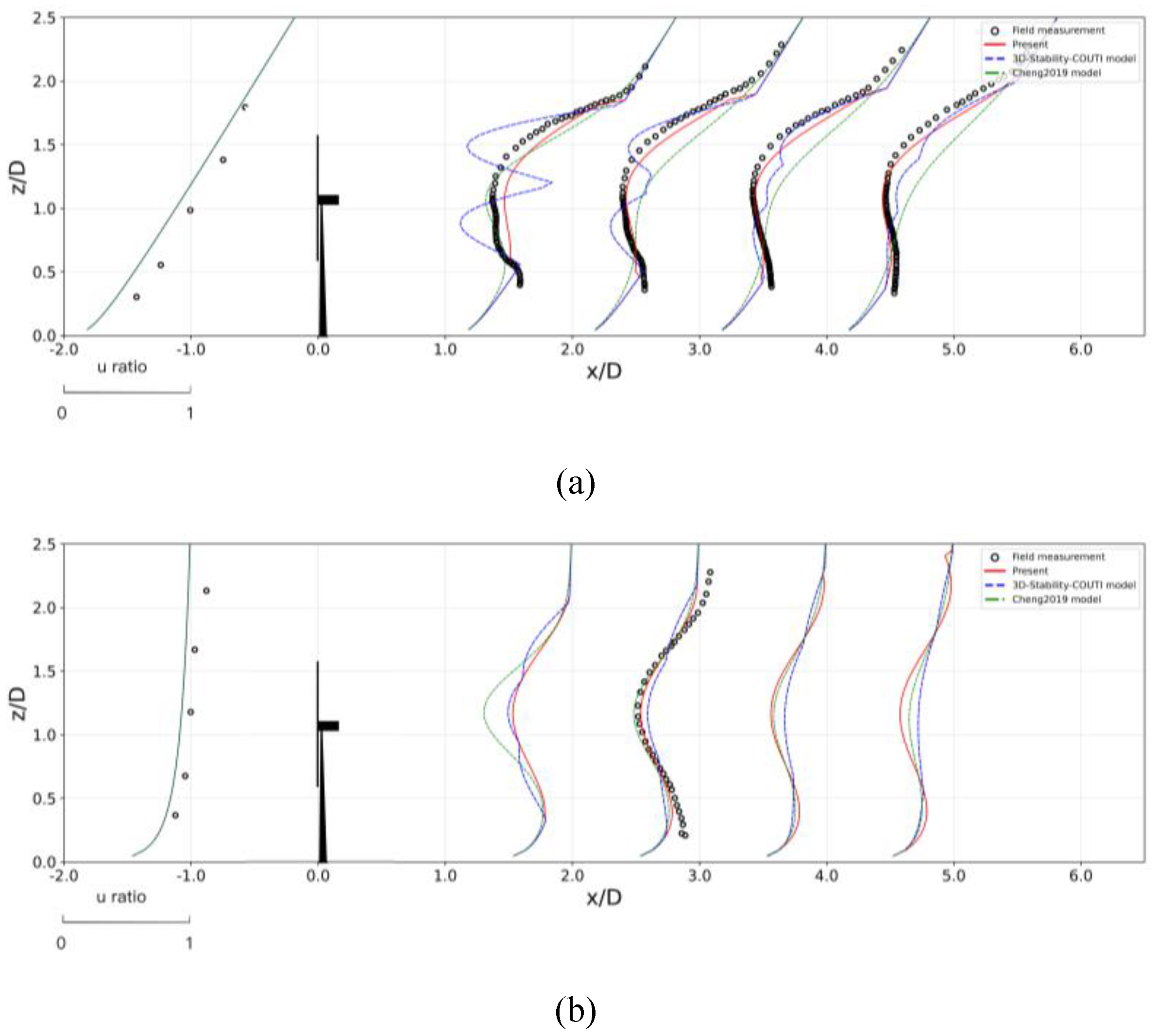
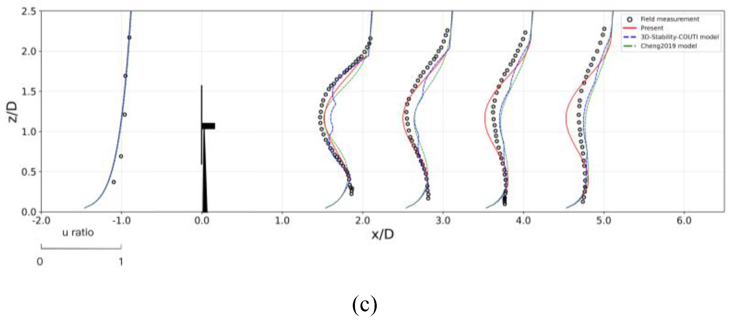
Figure 2.
Comparison of normalized wind speed profiles on the horizontal plane () for Case 1 under (a) stable, (b) unstable and (c) neutral atmospheric conditions.
Figure 2.
Comparison of normalized wind speed profiles on the horizontal plane () for Case 1 under (a) stable, (b) unstable and (c) neutral atmospheric conditions.
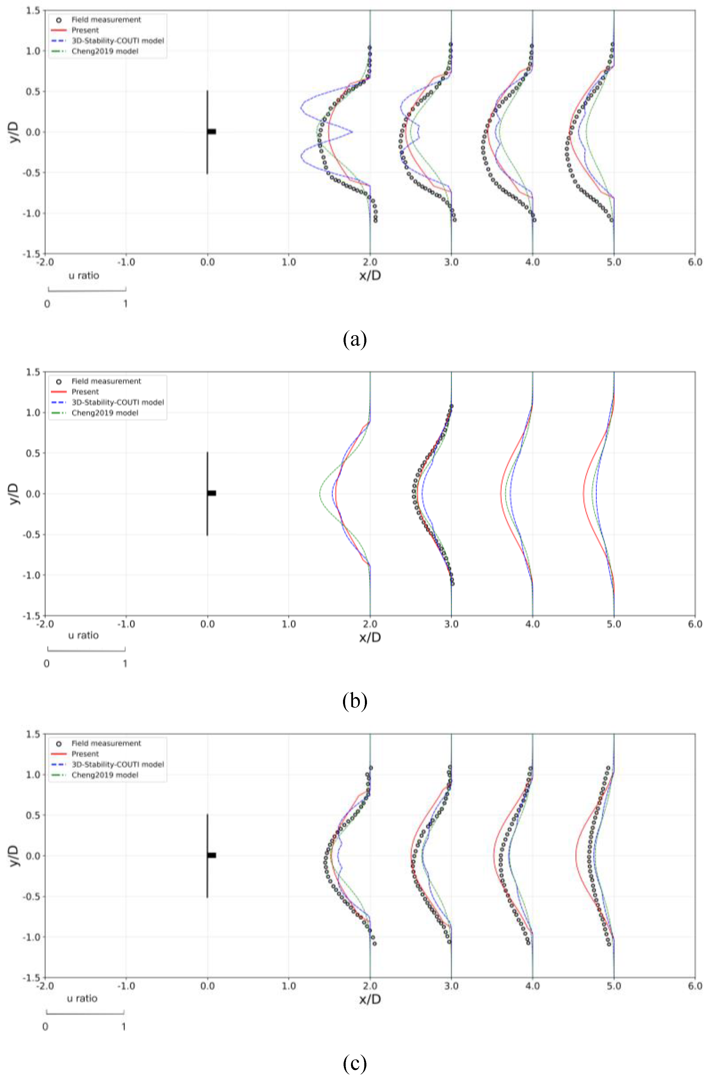
Figure 3.
Validation metrics of predicted normalized wind speed against field measurements of Case 1 for: (a) vertical profile at under stable atmopheric condition; (b) horizontal profile at under stable atmospheric condition; (c) vertical profile at under unstable atmopheric condition; (d) horizontal profile at under unstable atmospheric condition; (e) vertical profile at under neutral atmopheric condition; (f) horizontal profile at under neutral atmospheric condition.
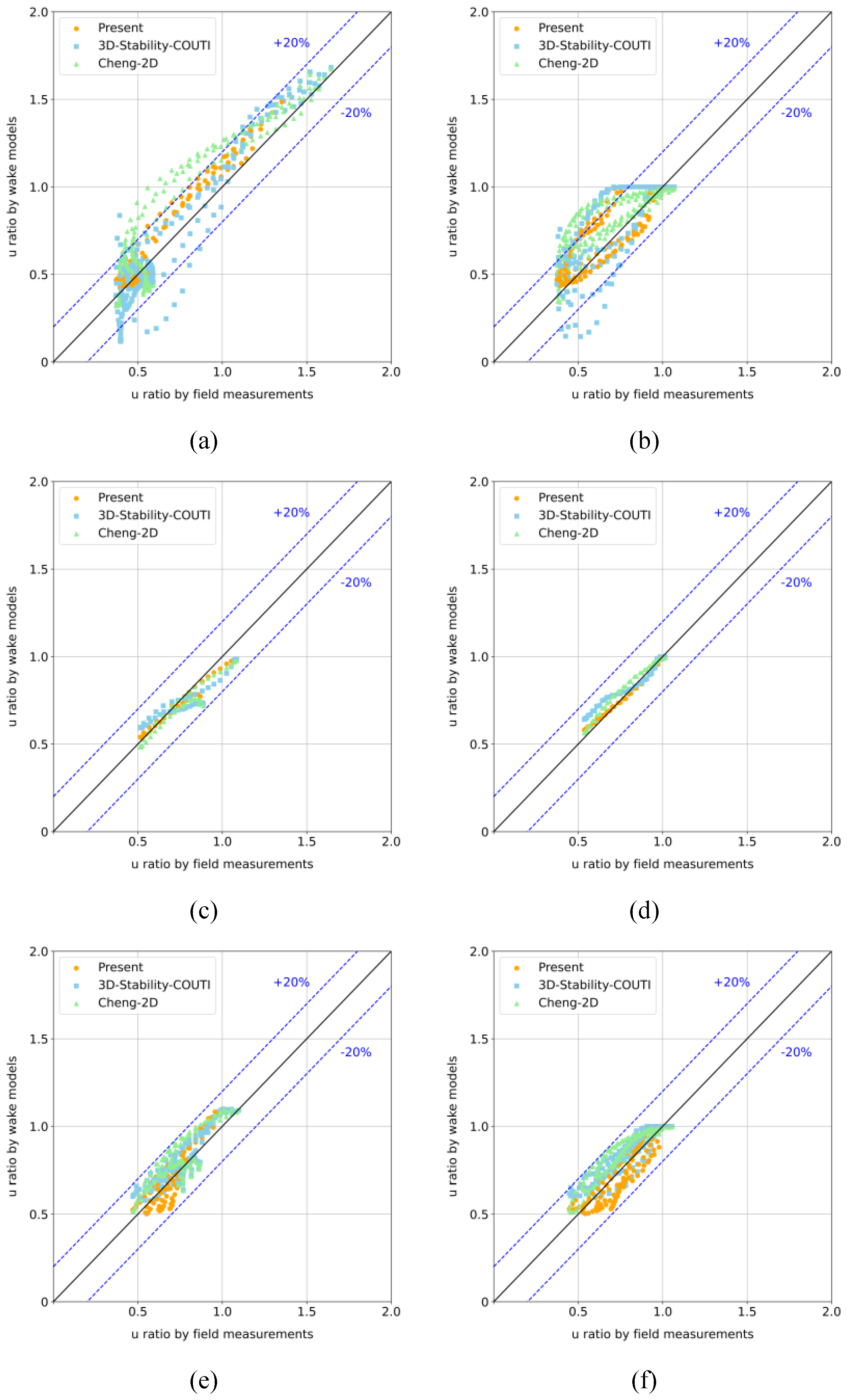
Figure 4.
Color maps of normalized wind speed on the horizontal place at hub height for Case 1 by (a) Present model under stable atmospheric condition; (b) Present model under unstable atmospheric condition; (c) 3D-Stability-COUTI model under stable atmospheric condition; (d) 3D-Stability-COUTI model under unstable atmospheric condition; (e) Cheng2019 model under stable atmospheric condition; (f) Cheng2019 model under unstable atmospheric condition.
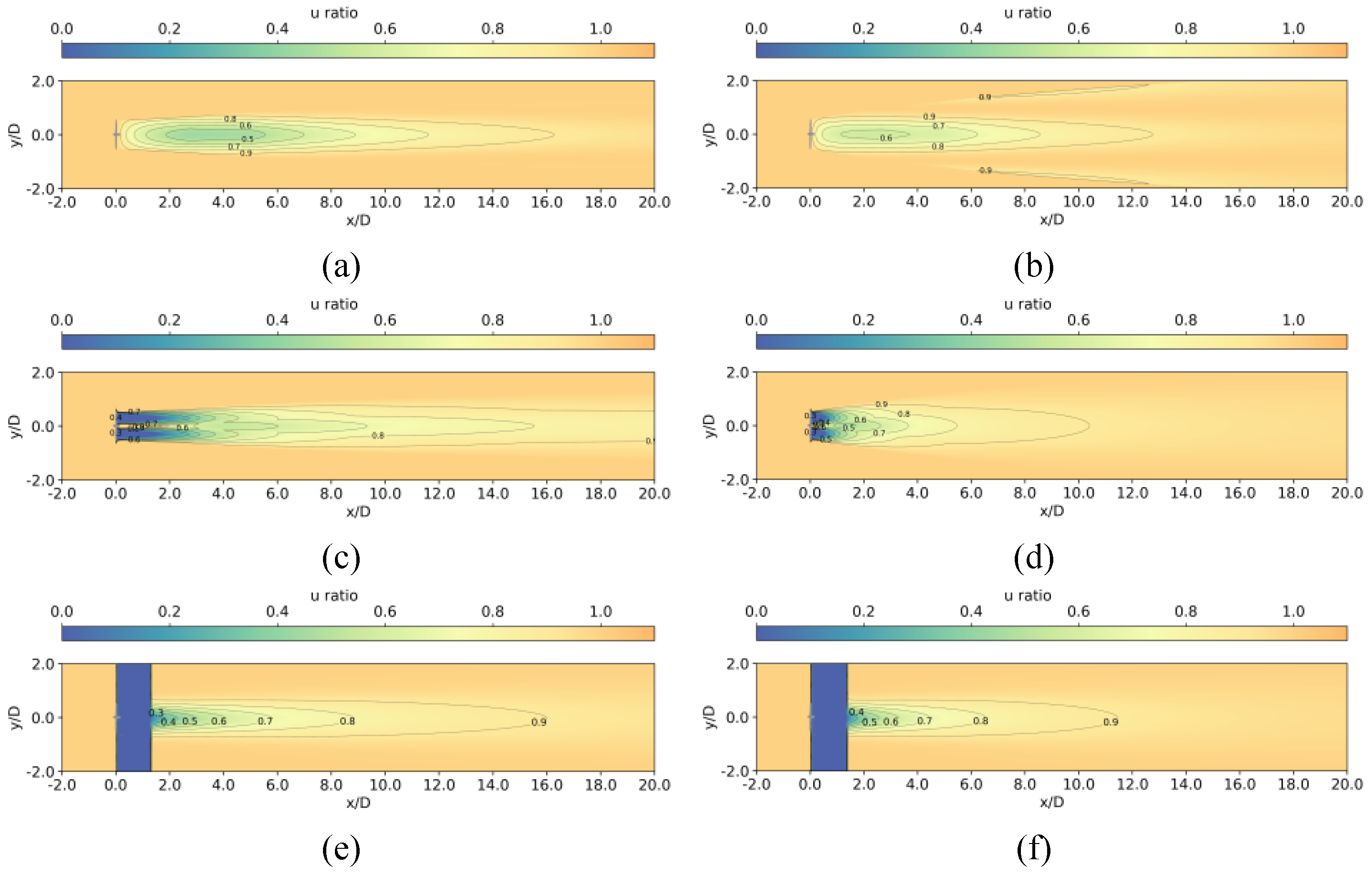
Figure 5.
Color maps of normalized wind speed on the vertical place at for Case 1 by (a) Present model under stable atmospheric condition; (b) Present model under unstable atmospheric condition; (c) 3D-Stability-COUTI model under stable atmospheric condition; (d) 3D-Stability-COUTI model under unstable atmospheric condition; (e) Cheng2019 model under stable atmospheric condition; (f) Cheng2019 model under unstable atmospheric condition.
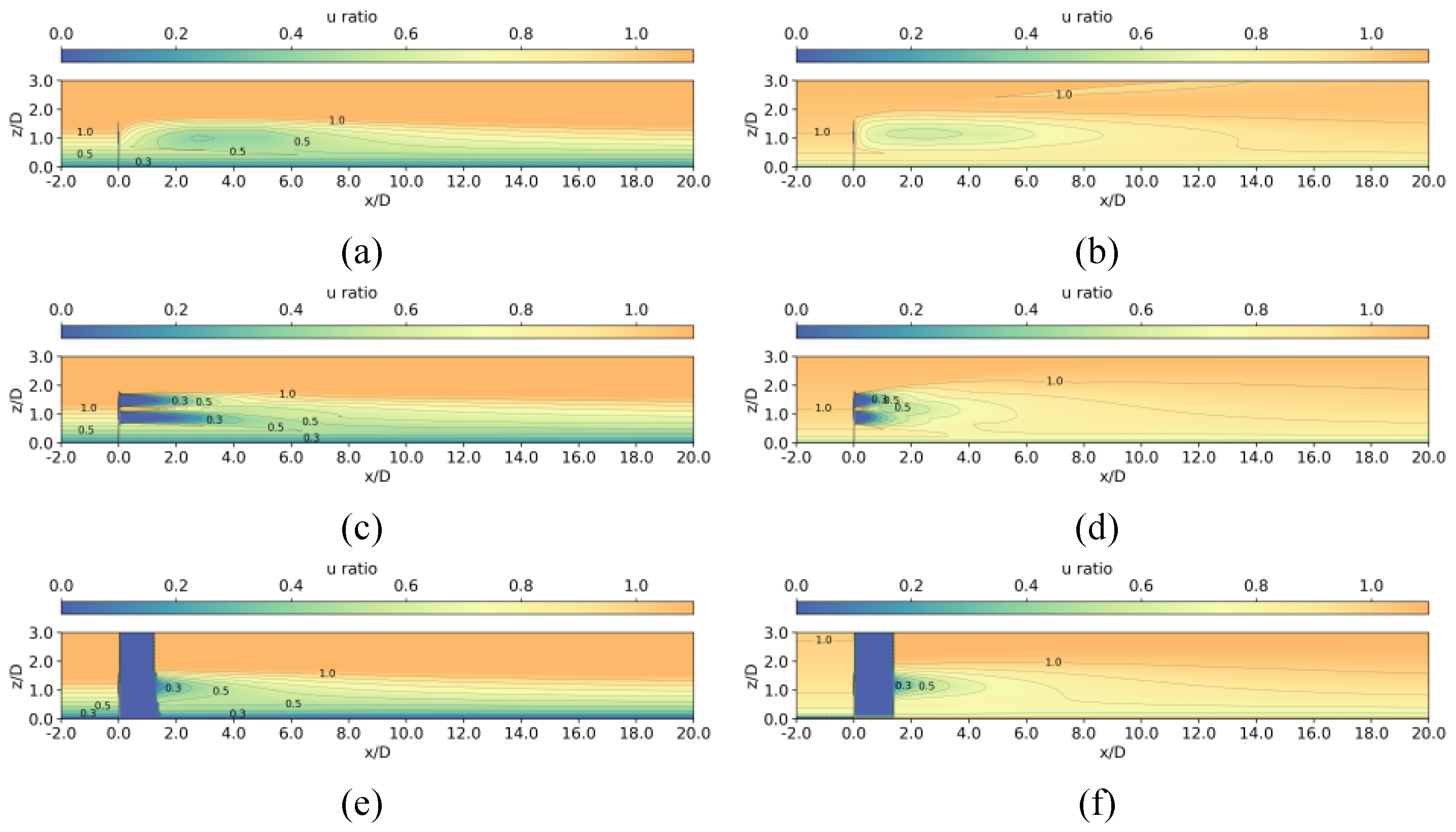
Figure 6.
Comparison of normalized wind speed profiles along the vertical centerline () for Case 2 under (a) stable and (b) unstable atmospheric conditions.
Figure 6.
Comparison of normalized wind speed profiles along the vertical centerline () for Case 2 under (a) stable and (b) unstable atmospheric conditions.
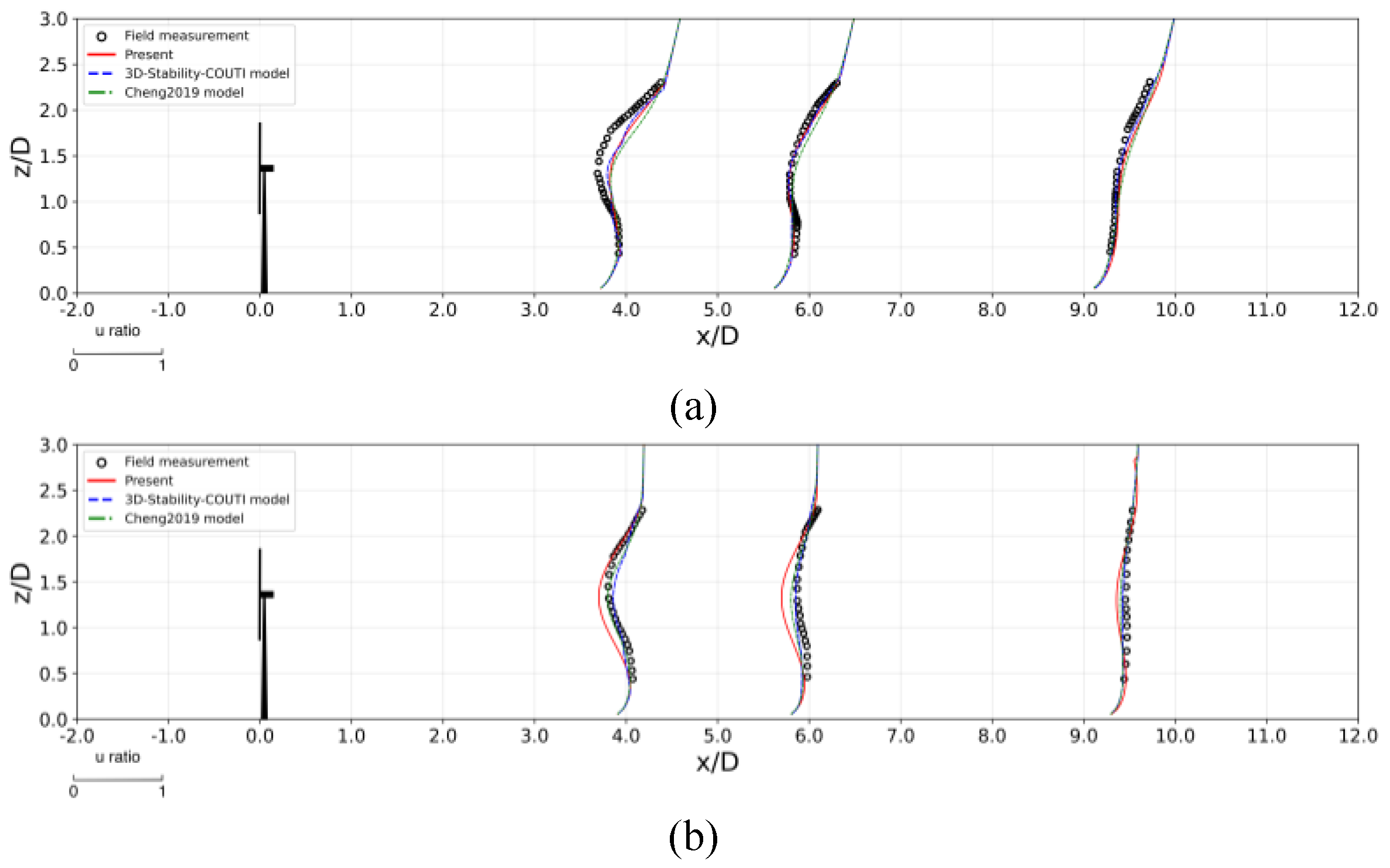
Figure 7.
Comparison of normalized wind speed profiles on the horizontal plane () for Case 2 under (a) stable and (b) unstable atmospheric conditions.
Figure 7.
Comparison of normalized wind speed profiles on the horizontal plane () for Case 2 under (a) stable and (b) unstable atmospheric conditions.
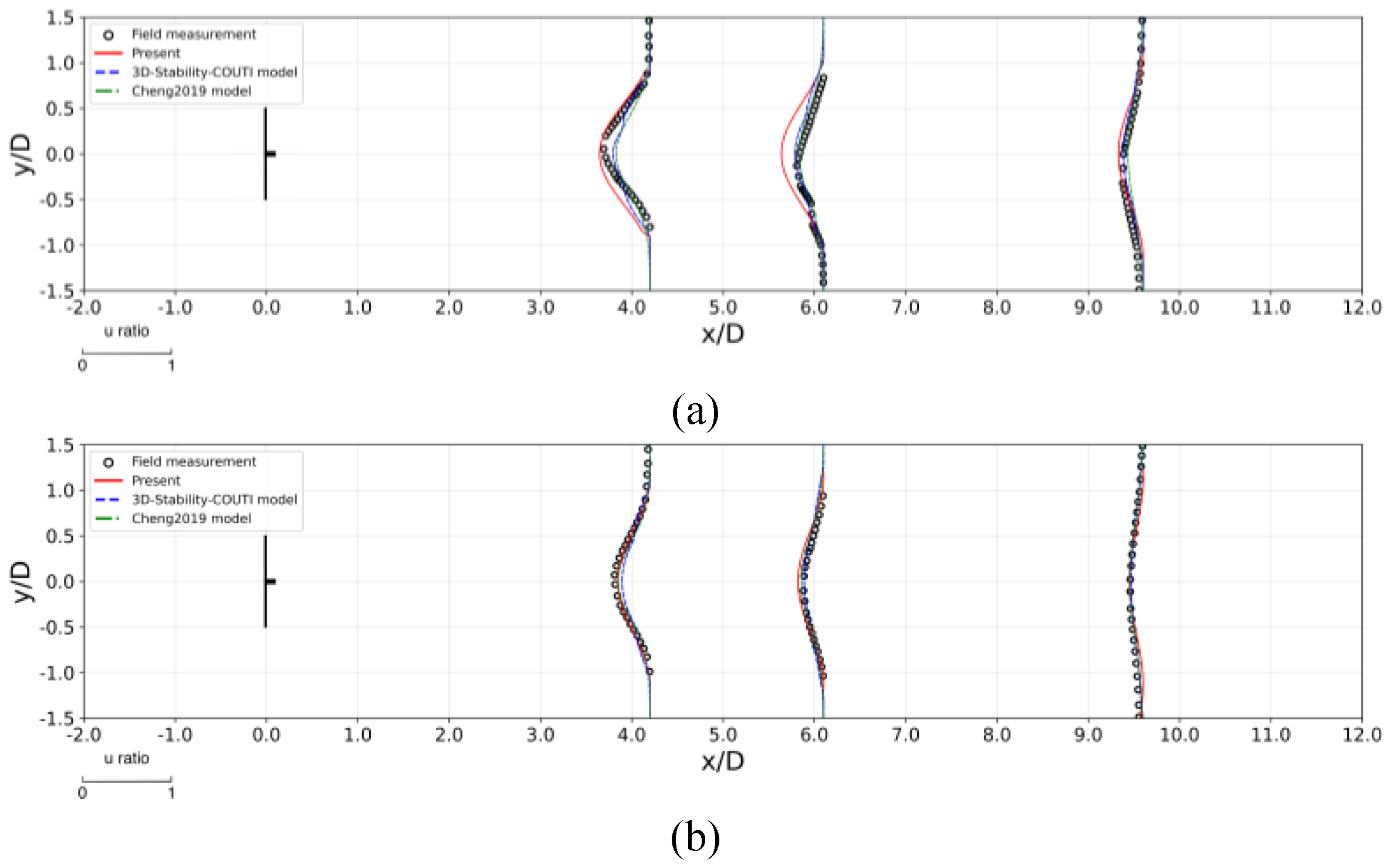
Figure 8.
Validation metrics of predicted normalized wind speed against field measurements of Case 2 for: (a) vertical profile at under stable atmopheric condition; (b) horizontal profile at under stable atmospheric condition; (c) vertical profile at under unstable atmopheric condition; (d) horizontal profile at under unstable atmospheric condition.
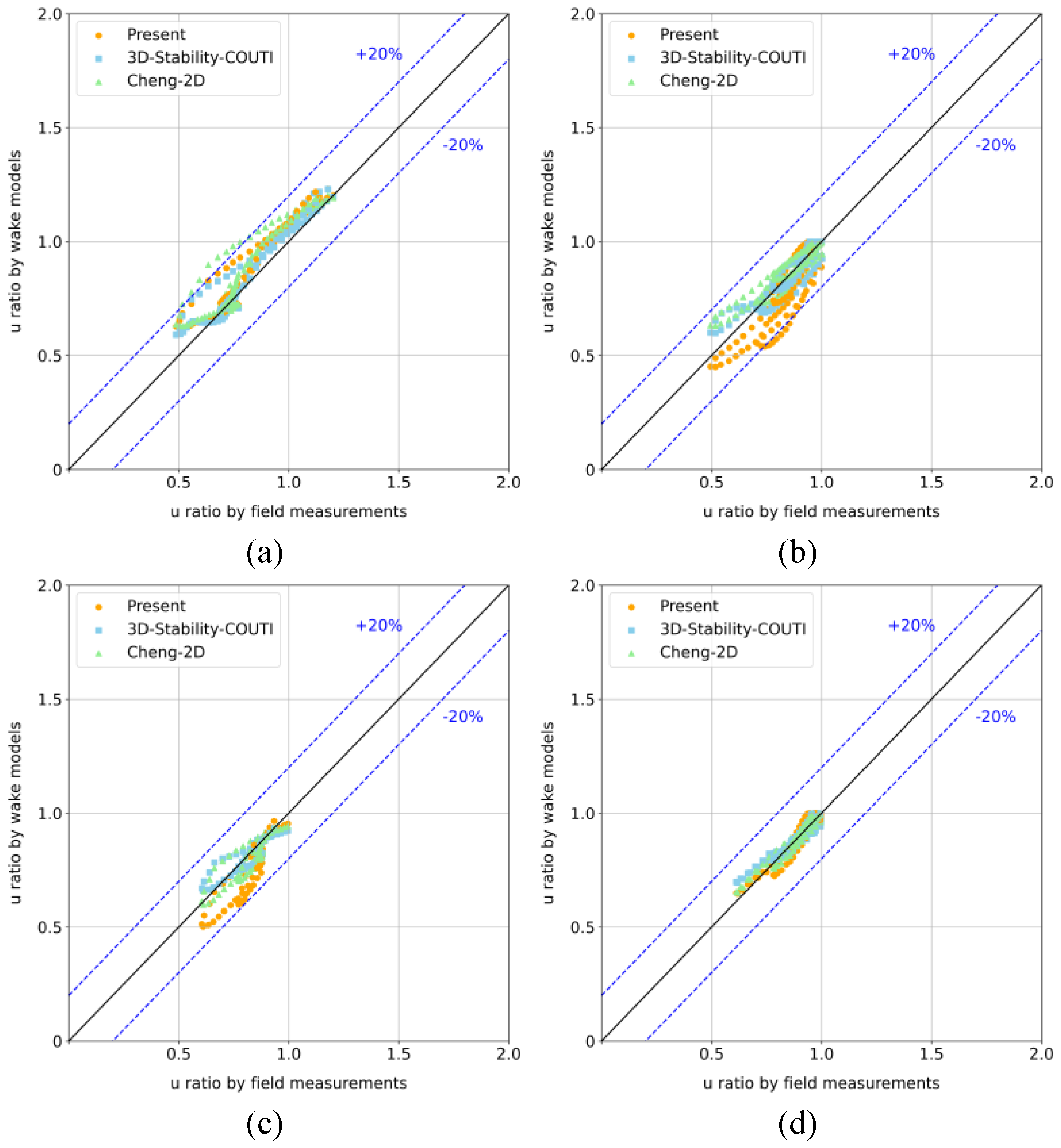
Figure 9.
Color maps of normalized wind speed on the horizontal place at hub height for Case 2 by (a) Present model under stable atmospheric condition; (b) Present model under unstable atmospheric condition; (c) 3D-Stability-COUTI model under stable atmospheric condition; (d) 3D-Stability-COUTI model under unstable atmospheric condition; (e) Cheng2019 model under stable atmospheric condition; (f) Cheng2019 model under unstable atmospheric condition.
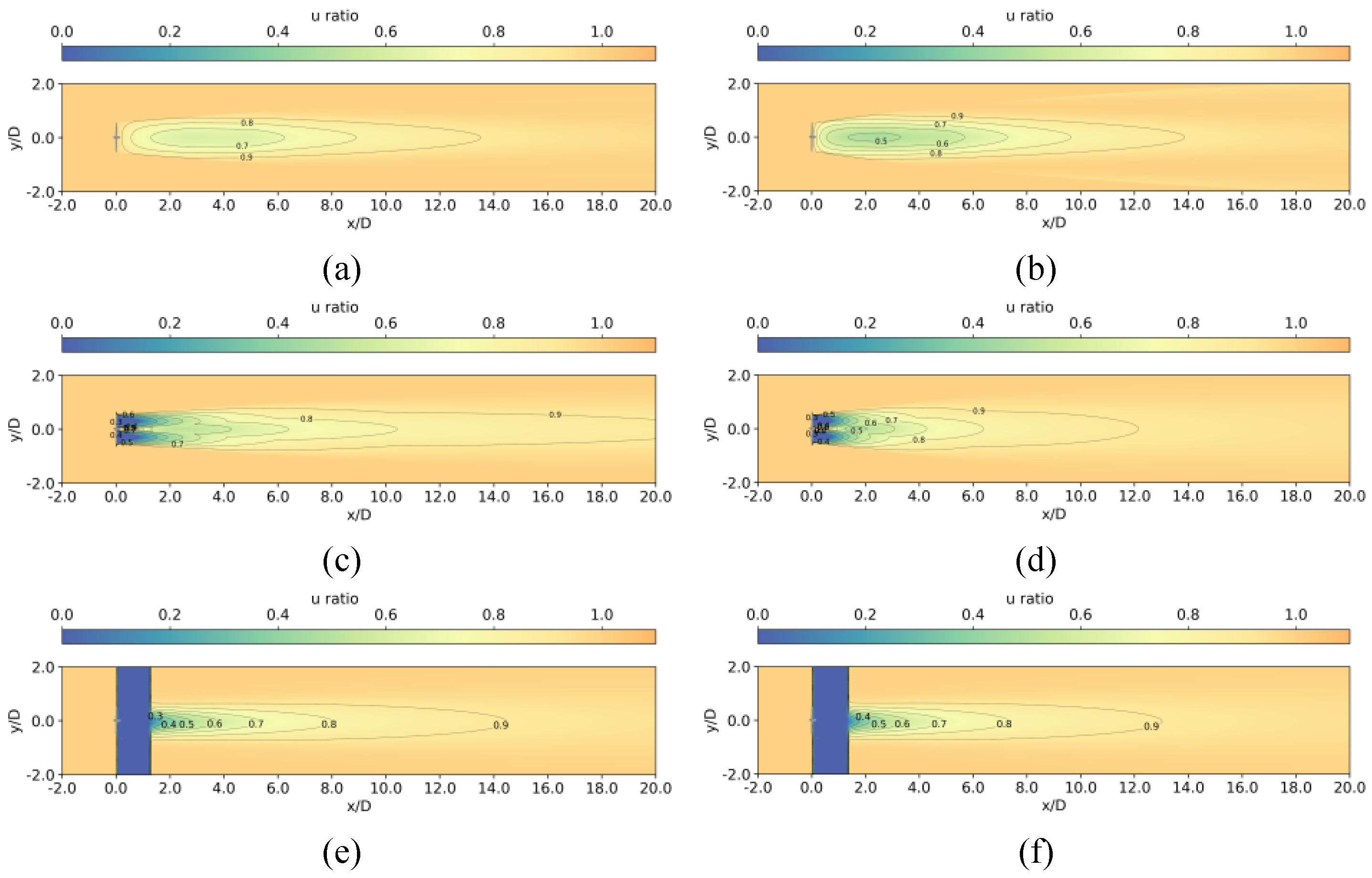

Table 1.
Key input parameters for the present wake model, the 3D-Stability-COUTI model [29] and the Cheng2019 model [28].
| Wake model considering atmospheric stability | Present wake model | 3D-Stability-COUTI model [29] | Cheng2019 model [28] | |
|---|---|---|---|---|
| WInd turbine | Rotor diameter, | ○ | ○ | ○ |
| Hub height, | ○ | ○ | ○ | |
| Thrust coefficient curve, | ○ | ○ | ○ | |
| Atmospheric inflow | Monin-Obukhov length, | ○ | ○ | ○ |
| Wind speed at hub height, | ○ | ○ | ○ | |
| Turbulence intensity at hub height, | ○ | ○ | ○ | |
| Terrain | Surface roughness length, | ○ | ○ | ○ |
| Angle of latitude, | × | × | ○ | |
Table 2.
Comparison of analytical formulas for wake models considering atmospheric stability.
| Wake model considering atmospheric stability | Proposed wake model | 3D-Stability-COUTI model [29] | Wake model based on Monin-Obukhov similarity theory [28] | ||
|---|---|---|---|---|---|
| Inflow | Incoming flow | Incoming wind velocity, |
where and |
where ; |
|
| Incoming turbulence intensity, |
where for and 7 for |
||||
| Wake model | Wake geometry | Width, |
where |
where ; ; ; ; |
|
| Wake velocity | Wake velocity, |
where velocity deficit, ; ; ; |
where velocity deficit, and ; ;;; |
where velocity deficit, and ; ; |
|
Table 3.
Summary of input parameters for Case 1 under neutral, unstable and stable atmospheric conditions.
Table 3.
Summary of input parameters for Case 1 under neutral, unstable and stable atmospheric conditions.
| Atmospheric stability | Stable | Unstable | Neutral |
|---|---|---|---|
| Rotor diameter, D(m) | 27 | 27 | 27 |
| Hub height, zH(m) | 32.1 | 32.1 | 32.1 |
| Wind turbine location, Φ (°) | 33.60795 | 33.60795 | 33.60795 |
| Surface roughness height, z0(m) | 0.0275 | 0.0275 | 0.0275 |
| Thrust coefficient, Ct | 0.83 | 0.81 | 0.70 |
| Wind speed at hub height, UH | 4.8 | 6.7 | 8.7 |
| Turbulence intensity at hub height, IH |
0.034 | 0.126 | 0.107 |
| Obukhov length, L(m) | 8.69 | -112.36 | 2500 |
Table 4.
Hit rates of predicted wind speed against field measurements of Case 1 by Present model, 3D-Stability-COUTI model and Cheng2019 model.
Table 4.
Hit rates of predicted wind speed against field measurements of Case 1 by Present model, 3D-Stability-COUTI model and Cheng2019 model.
| Hit rate | Atmospheric stability | Plane | Present model | 3D-Stability-COUTI | Cheng2019 |
|---|---|---|---|---|---|
| stable | XOZ | 0.94 | 0.83 | 0.73 | |
| XOY | 0.73 | 0.59 | 0.65 | ||
| unstable | XOZ | 0.97 | 0.97 | 0.97 | |
| XOY | 1.00 | 1.00 | 1.00 | ||
| neutral | XOZ | 0.98 | 0.99 | 0.87 | |
| XOY | 0.96 | 0.95 | 0.87 | ||
| stable | XOZ | 0.99 | 0.91 | 0.82 | |
| XOY | 0.87 | 0.69 | 0.74 | ||
| unstable | XOZ | 1.00 | 1.00 | 1.00 | |
| XOY | 1.00 | 1.00 | 1.00 | ||
| neutral | XOZ | 1.00 | 1.00 | 1.00 | |
| XOY | 1.00 | 1.00 | 1.00 |
Table 5.
Summary of input parameters for Case 2 under neutral, unstable and stable atmospheric conditions.
Table 5.
Summary of input parameters for Case 2 under neutral, unstable and stable atmospheric conditions.
| Atmospheric stability | Stable | Unstable |
|---|---|---|
| Rotor diameter, D(m) | 23 | 23 |
| Hub height, zH(m) | 31 | 31 |
| Wind turbine location, Φ (°) | 57.47467 | 57.47467 |
| Surface roughness height, z0(m) | 0.0005 | 0.0005 |
| Thrust coefficient, Ct | 0.82 | 0.82 |
| Wind speed at hub height, UH | 8.0 | 8.0 |
| Turbulence intensity at hub height, IH |
0.085 | 0.085 |
| Obukhov length, L(m) | 35 | 100 |
Table 6.
Hit rates of predicted wind speed against field measurements of Case 2 by Present model, 3D-Stability-COUTI model and Cheng2019 model.
Table 6.
Hit rates of predicted wind speed against field measurements of Case 2 by Present model, 3D-Stability-COUTI model and Cheng2019 model.
| Hit rate | Atmospheric stability | Plane | Present model | 3D-Stability-COUTI | Cheng2019 |
|---|---|---|---|---|---|
| stable | XOZ | 0.93 | 0.97 | 0.89 | |
| XOY | 0.83 | 1.00 | 0.99 | ||
| unstable | XOZ | 0.90 | 1.00 | 1.00 | |
| XOY | 1.00 | 1.00 | 1.00 | ||
| stable | XOZ | 1.00 | 1.00 | 0.93 | |
| XOY | 0.93 | 1.00 | 1.00 | ||
| unstable | XOZ | 1.00 | 1.00 | 1.00 | |
| XOY | 1.00 | 1.00 | 1.00 |
Disclaimer/Publisher’s Note: The statements, opinions and data contained in all publications are solely those of the individual author(s) and contributor(s) and not of MDPI and/or the editor(s). MDPI and/or the editor(s) disclaim responsibility for any injury to people or property resulting from any ideas, methods, instructions or products referred to in the content. |
© 2025 by the authors. Licensee MDPI, Basel, Switzerland. This article is an open access article distributed under the terms and conditions of the Creative Commons Attribution (CC BY) license (http://creativecommons.org/licenses/by/4.0/).
Copyright: This open access article is published under a Creative Commons CC BY 4.0 license, which permit the free download, distribution, and reuse, provided that the author and preprint are cited in any reuse.


